


I. INTRODUCTION
Excellent theoretical and experimental works, most of them from the last decade, have successfully defined the analytical background for inductive power transfer (IPT) and confirmed it as a feasible and effective way of transferring power in the mW to kW ([Reference Mirbozorgi, Bahrami, Sawan and Gosselin1 ] and [Reference Choi, Huh, Lee and Rim2], respectively) range under appreciable separation distance between source (emitter or primary) and load (receiver or secondary).
Currently, however, IPT solutions face different challenges, all of them very much related to practical implementation issues:
-
(a) Misunderstanding of General Concepts – Among practitioners and the scientific community not completely aware of IPT latest advances, inductive transfer has been inadvertently rejected under the claim of low efficiency: partially due to inherent (but reducible) switching and conduction losses of the apparatus driving primary coils; partially due to the lack of understanding of general concepts related to the weakly coupled inductor systems and how power flow is established between primary and secondary. The “low efficiency” argument, however, is an allegation that several papers have proved wrong [Reference Wu, Gilchrist, Sealy and Bronson3].
-
(b) Operational Safety Issue – From time to time (with emphasis in recent literature), IPT solutions are questioned in terms of the effects of time-varying electric and magnetic fields over objects and organic matter in the surroundings of a converter [Reference Christ4]. This happens because frequencies involved in wireless/IPT range from tens of kHz to tens of MHz. Associated with the diversified IPT power range, this defines a considerably large spectrum where different possible biological and electromagnetic effects may fit.
-
(c) Coupler Design Issue – The design of inductive couplers in terms of physical size (as a function of transferred power) and relative spatial positioning between primary and secondary is not straightforward. Typically it demands deep knowledge on analytical approaches [Reference Jonah, Merwaday, Georgakopoulos and Tentzeris5] and mathematical modeling (attributes that may not be promptly available in all expertise levels) or a powerful numerical solver (e.g. three-dimensional (3D) finite element method (FEM) solvers for electromagnetics) able to model, simulate, and extract data for a particular coupler configuration. The difficulty with this later possibility is that 3D FEM is rarely available outside the specialized scientific/engineering community or industry;
The authors of the present work are prone to think that each of these arguments is partially contributing to slow down wide adoption of IPT outside the academic circle and may be discouraging practitioners and non-IPT-specialized engineers to propose novel ideas, solutions and to integrate IPT couplers (even the most basic ones) into already existing products. Thus, these three arguments are the motivation of this paper and contributions are proposed to solve each one.
Contributions to determine physical size of couplers are already available in literature, but in limited quantity. A sizing method for pads used in electric vehicle (EV) systems was presented in [Reference Nagendra, Covic and Boys6] with focus on structures like the Double-D (DD) and the Double-D Quadrature (DDQ), as reviewed by [Reference Fisher, Farley, Gao, Bai and Tse7]. This approach employs the 3D magnetic modeling software and aims to provide an initial solution (a “ball-park”) that satisfies a set of given operating parameters and spatial restrictions. This initial solution can be later optimized by introducing small geometrical modifications to improve magnetic flux distribution or copper usage. In [Reference Arteaga, Iturralde, Ibanez and Elosegui8], an analytical approach is depicted, again aiming to determine width and length of a simple coupler subjected to initial constraints. Both cases however are inherently associated with the problems described in argument (c) and are based on comparisons between the new desired coupler and a previously designed coupler with similar concept (a reference design). The reference design by itself is mostly achieved by trial and error.
Also, there are records in literature related to numerical design procedures, as seen in [Reference Inoue, Nagashima, Wei and Sekiya9, Reference Sekiya, Ezawa and Tanji10], which combine exact resonant circuit equations to express the converter in terms of optimized efficiency and improved L–C parameter selection to ensure soft-switching. These approaches however do not consider the design of couplers and are limited to the electrical circuit.
Thus, the present paper proposes a different approach, which uses a free two-dimensional (2D) FEM and a set of C programmed routines to iteratively represent couplers based on user inputs and restrictions. By replacing the 3D FEM solver with a free 2D solver, one removes the cost and availability barriers imposed by the first tool. Also, since computational resources necessary to quickly perform an accurate 2D FEM run are much smaller than those required by a typical 3D solver, this new approach is suitable for basic home/office computers.
In this proposal, the C routines developed in MatLab interact directly with the 2D solver, editing and guiding the coupler geometry design process until it reaches a solution that satisfies initial parameters. Routines are also available for optimization and for comprehensive data extraction. A dedicated routine analyzes magnetic field intensity in the surroundings of the designed coupler and compares results with reference international standards, graphically illustrating the area under influence of the converter and if magnetic field exposure limits are acceptable or not. No previous FEM knowledge is necessary to use this approach since mesh sizes, boundary conditions, and other particular parameters are automatically adjusted by the routines based on particularities of IPT designs.
Along the paper, routines are described, limitations are commented and experimental results are discussed.
II. EXHAUSTIVE DESIGN ALGORITHMS
An Exhaustive Design Algorithm (EDA) is defined in this work as a sequence of commands that act as a pre-processor and/or a post-processor for the 2D FEM solver. The term “exhaustive” emphasizes the iterative nature of the procedure and is also due to the fact that there is no theoretical prediction of which coupler dimensions may serve as a solution to the user inputs, thus being necessary to perform several FEM runs to reach an admissible solution or to find out that a coupler geometry is not possible under the given restrictions.
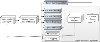
Figure 1 shows is a schematic overview of the computational tool (that can be understood as a MatLab toolbox) including all EDAs (the five shaded blocks). Every design must begin from Basic Routine that manages and gathers user inputs and also control all other routines. Later, solid or stranded windings can be defined manually or designed with user-defined parameters (currents, frequency, and current density). This algorithm is not discussed in this work due to its relative simplicity.
Block diagram of all EDAs and complementary routines.

A) Generic exhaustive algorithm structure
These algorithms have pre-processing, processing and post-processing steps. The pre-processing phase creates and edits geometric entities such as lines segment, arc segments, and nodes within a 2D finite element simulation domain (Ω 2D ), assign material properties, defines mesh dimensions and boundary conditions. Thus, the pre-processing phase literally draws the coupler before Ω 2D is discretized and simulated by the solver. The drawing containing the coupler geometry is updated based in results obtained in previous iterations.
The solver employed here is FEMM (Finite Element Method Magnetics) [Reference Meeker11], a well-known and powerful free software which uses the variational formulation and first-order triangle elements to solve Ω 2D . Commands used as interface between MatLab and FEMM are described in the documentation of [Reference Meeker11]. For reference and to make clear the limitations of the numerical method, mathematical formulation is presented.
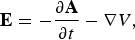
The magnetic flux density vector, B, is given in (1) as a function of the magnetic vector potential, A. Substituting (1) in differential form of Faraday's Law of Induction results in (2), which can be integrated to yield (3). Finally, considering Ohm's Law in vector notation, (4) is written. E is the electric field intensity vector, J src represents current sources, V is a scalar denoting voltage, μ(B) indicates that non-linear magnetic permeability is taken into account and σ the electrical conductivity [Reference Meeker11].
 $${\bf B} = \nabla \times {\bf A}, $$
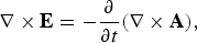 $$\nabla \times {\bf E} = - \displaystyle{\partial \over {\partial t}}(\nabla \times {\bf A}),$$
 $${\bf E} = - \displaystyle{{\partial {\bf A}} \over {\partial t}} - \nabla V,$$
 $$\nabla \times \left( {\displaystyle{1 \over {\mu ({\bf B})}}\nabla \times {\bf A}} \right) = - \sigma \displaystyle{{\partial {\bf A}} \over {\partial t}} + {J_{src}} - \sigma \nabla V.$$
With minor modifications, (4) is used by the software in time-harmonic problems with one single angular frequency ω (which is enough for IPT since resonant converters in fact should provide sinusoidal excitation to the primary coil at the resonant frequency ω 0 = 2πf 0 only. Anyway, this is known as first-harmonic approximation). One might observe that the above formulation ignores displacement currents and as a result, FEMM can only be applied if this effect is negligible. Fortunately, this is the case of IPT converters which employ good electrical conductors and satisfy the condition σ ≫ ωε med [Reference Arthur12], where ε med is the electrical permittivity of the medium (typically air). For instance, consider permittivity of vacuum ε 0 = 8.85 × 10⁻¹² F.m−1, relative permittivity of air ε r = 1, ε med = ε 0 ε r , and for copper σ = 5.96 × 10⁷ S.m−1. With frequency ranging from 60 Hz to 10 MHz, there is 3.34 × 10⁻⁹ ≤ ωε med ≤ 5.56 × 10⁻⁴. Thus, σ ≫ ωε med for IPT applications commonly reported.
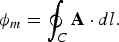
One of the advantages of the formulation shown in (1) is that flux lines are simply plots if the magnetic potential vector A. Thus, inductance (self and mutual) is easily obtained as L x = ϕ m /Ix , being I x the peak excitation current, since peak mutual flux ϕ m is given according to (5). Here x = p if it refers to primary inductor and x = s if refers to secondary inductor. This indicates that the line integral is taken over the boundary of the surface, defined by the target coil geometry. The boundary is here denoted by C, while dl is the differential straight conductor filament. Note that all voltages, currents, and fluxes expressed in this paper are peak values.
 $${\phi _m} = \oint_C {\bf {A}} \cdot dl. $$
To eliminate the influence of nearby coils during the EDA execution and to determine self-inductances correctly, all currents are set to a null value, except in the coil under study, for which is assigned peak current (in order to allow the evaluation of saturation in high-permeability cores, if they exist). EDA are divided into two main approaches: Target inductance (TI) and target output (TO) algorithms.
B) TI algorithms
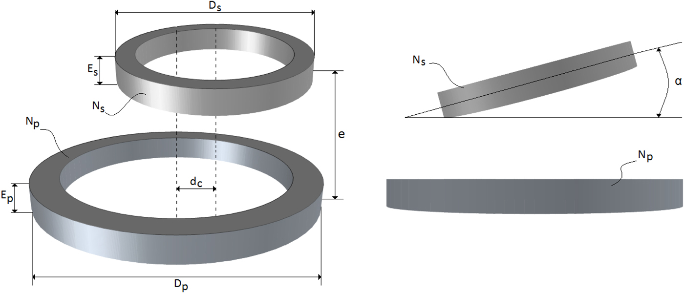
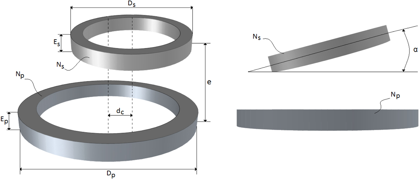
TI algorithms seek for a user-defined self-inductance for primary and secondary not considering the influence of one over the other. Mutual inductance (M), secondary open-circuit voltage (V oc ), secondary short-circuit current (I sc ), and uncompensated output power (S u ) are obtained as consequences of TIs. For all algorithms shown axisymmetric modeling is used when performing FEM simulations. For geometric parameters mentioned in next sections, consider Fig. 2.
Geometric parameters.
1) LUMPED CIRCULAR COILS, FIXED NUMBER OF TURNS
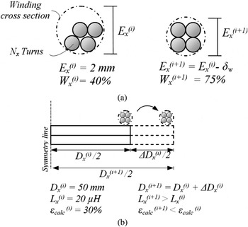
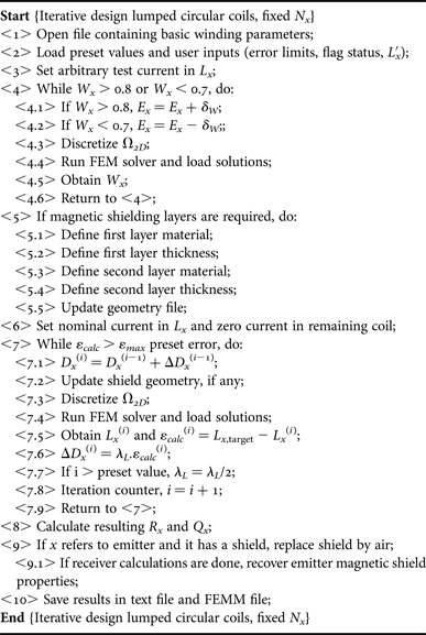
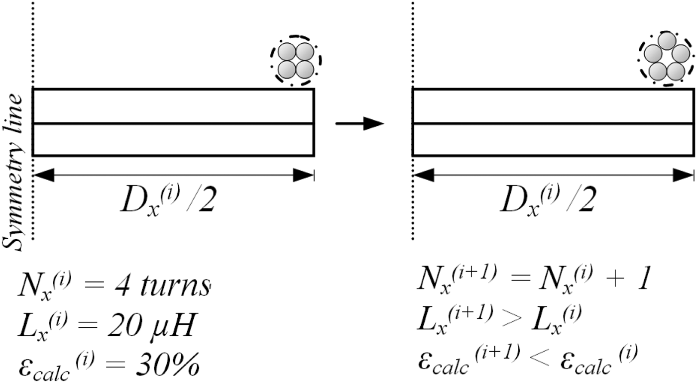
This procedure, shown in Algorithm I, seeks for the TI L x,target when the user defines the number of turns N x . Since N x is fixed and a lumped coils is being designed, the algorithm draws a circle of diameter E x that contains all N x turns (each one with the properties obtained in step <1>, from the winding design routine shown in Fig. 1) with a winding factor 0.7 ≤ W x ≤ 0.8. W x = 0.75 means that 75% of the winding cross-section is filled up by copper and 25% is filled by air. Values between 70 and 80% usually guarantee simultaneously a good area usage and practical implementation. This is shown in steps <4.1> to <4.6>. Figure 3(a) illustrates the W x adjust loop with a fixed step δ W (e.g. δ W = 0.1 mm).
Details for Algorithm I, (a) winding fill factor, W x , iterative adjust procedure and (b) main loop with arbitrary values shown.

Lumped circular coils, fixed N x .
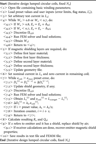
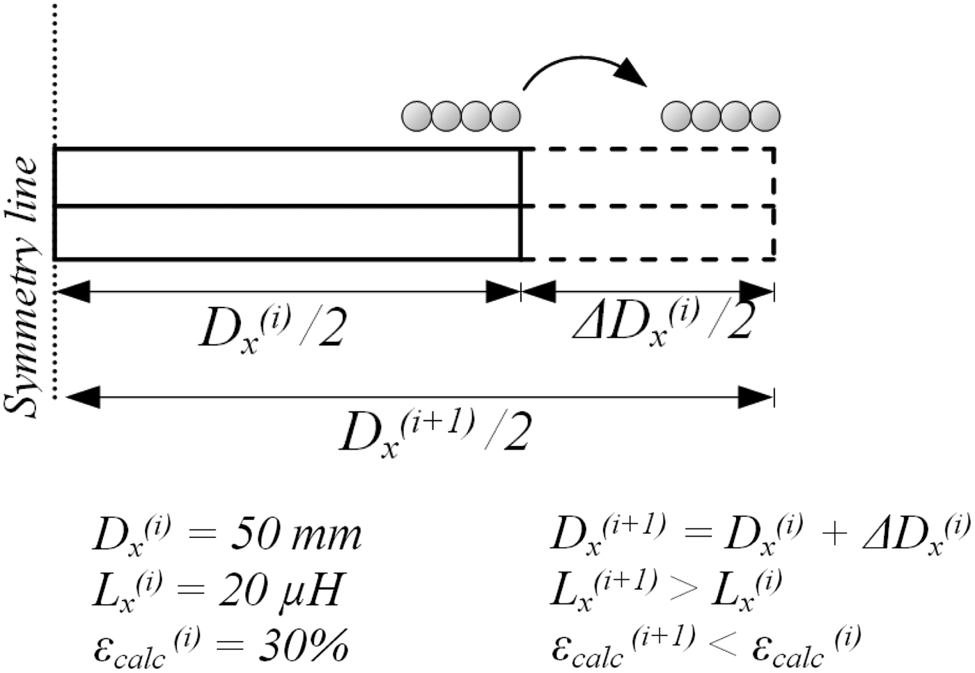
With the winding cross-section defined, the only variable that can be used to pursue L x,target is the coil diameter, D x , which is varied based in a diameter step ΔD x (i−1), defined in the previous iteration (i − 1) considering ε calc (i), (the error between L x,target and calculated L x ) and also a pre-defined scalar error gain λ L , that ensures fast convergence. When iteration counter i, reaches a maximum iteration number without a final solution for L x,target , λL is updated in order to force the algorithm to continue. All this define the main loop, as shown in steps <7.1> to <7.9>.
Figure 3(b) illustrates the main loop, that is finalized when ε calc (i) is less than a given precision, ε max . At this moment, resulting inductor series resistance R x and unloaded quality factor Q x = ωL x /R x is calculated from the FEM solver. All inductance calculations are performed using the magnetic materials desired and defined by the user in step <5.1> to <5.5>. When it comes to the time to design the secondary coil, magnetic materials of the primary (if any) are neutralized to avoid their influence over the secondary reluctance path. Thus, one can note that this algorithm seek for the target self-inductance without considering the effect of a nearby structure.
2) LUMPED CIRCULAR COILS, FIXED DIAMETER
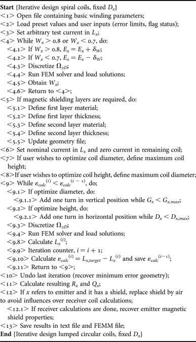
This represents a coil system with mechanical restriction being D x the target diameter. The procedure depicted in Algorithm II.
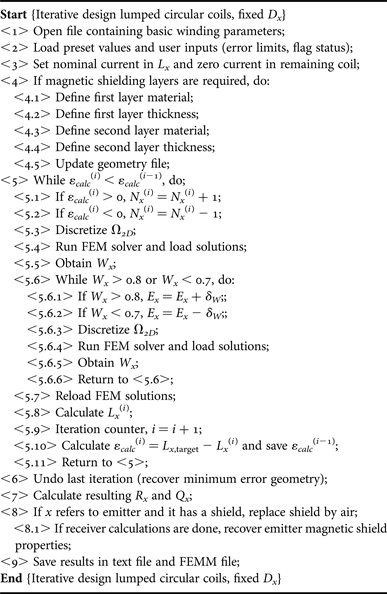
Lumped circular coils, fixed D x .
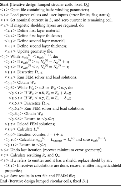
In this case, N x is the adjustable variable and it is incremented or decremented in step <5.1> or <5.2> depending on the sign of ε calc (i). Each time N x is modified, the cross-section of the coil is checked to ensure 0.7 ≤ W x ≤ 0.8.
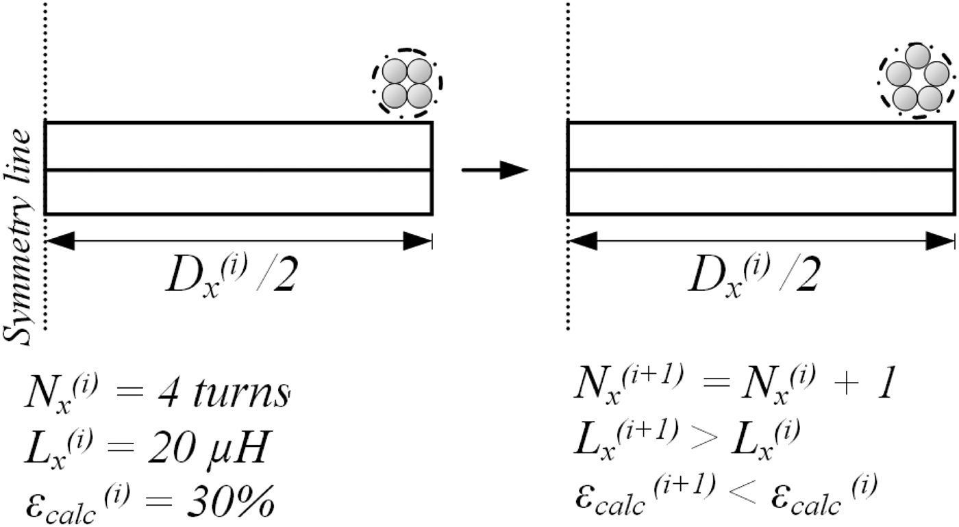
The main loop from <5.1> to <5.11> includes the W x loop. Since N x can only assume integer values (no fractional turn allowed), it may occur that an increment results in ε calc (i) > ε calc (i − 1). Thus, the main loop is finalized when the error increases between successive iterations and the geometric configuration of the iteration with lowest calculated error are maintained. Figure 4 illustrate this algorithm.
Details for Algorithm II, main loop with arbitrary values shown.
3) SPIRAL COILS, FIXED NUMBER OF TURNS
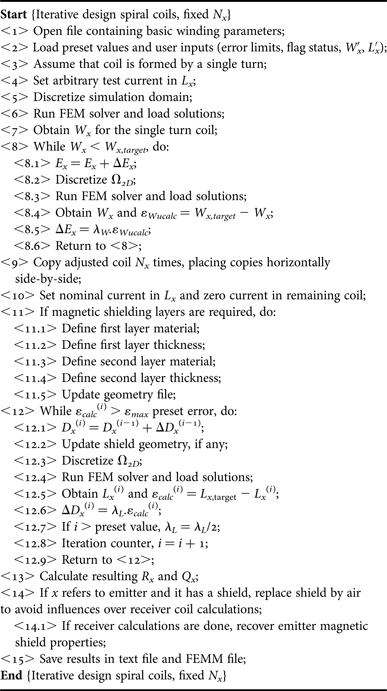
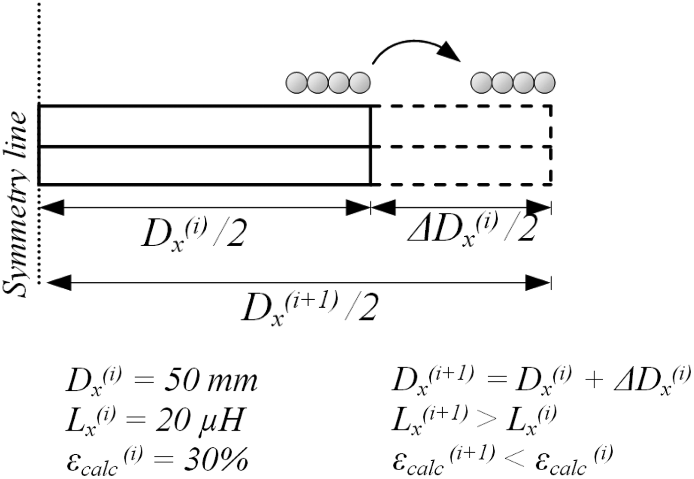
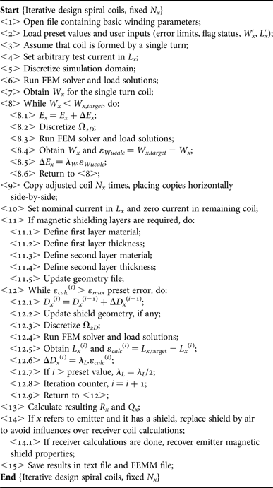
Spiral coils are a particular case of circular coils. The algorithm for this kind of winding begins by defining the cross-section of one single turn based on the wire properties obtained in an earlier routine. W x is adjusted once (based on a target W x,target ) and the resulting cross-section is replicated side-by-side N x times.
The winding fill factor loop in this case was implemented with a strategy similar to that seen in Algorithm I, main loop, that is to vary E x according to ΔE x (which is calculated with W x error ε Wu,calc and a scalar winding error gain λ W . This was done to indicate to possible users that they can add and modify sub-routines. The main loop is illustrated in Fig. 5.
Details for Algorithm III, main loop with arbitrary values shown.
Spiral coils, fixed N x .
4) SPIRAL COILS, FIXED DIAMETER
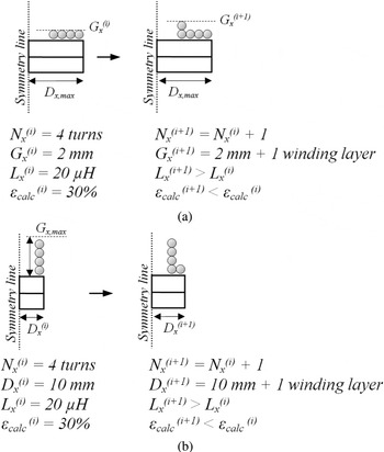
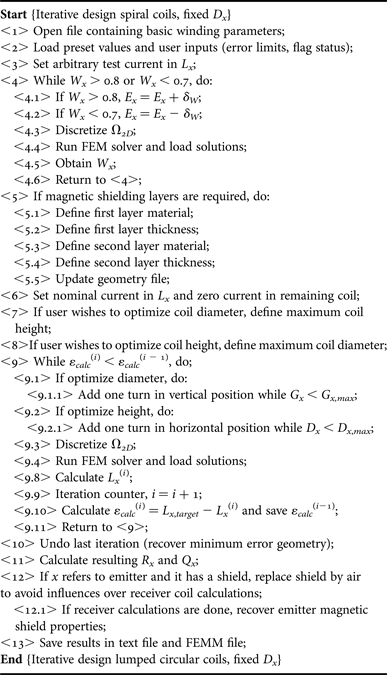
This case can be used to include a different mechanical restriction approach, where D x is understood as maximum diameter, D x,max , and not as target diameter (as was the case in Algorithm II). After W x is adjusted in steps <4.1> to <4.6>, the user has the option to add turns in horizontal direction or in the vertical direction. In the first possibility, D x is increased significantly while coil height is kept fixed. If maximum diameter is reached and L x,target was not found, one vertical layer is added.
In the second possibility, total coil height G x = N x Ex is increased, while G x < G x,max . If L x,target was not found, one horizontal layer is added. So, it is possible to control the algorithm design method in order to achieve various coil shapes. Main loop alternatives are represented in Figs 6(a) and 6(b).
Details for Algorithm IV, (a) total coil height optimization and (b) coil diameter optimization.

Spiral coils, fixed D x .
5) ADDITIONAL ALGORITHMS
After any of the iterative procedures is completed, the user may wish to characterize couplers in terms of axial (or vertical), lateral (or horizontal), and/or angular misalignment, since IPT solutions are usually subjected to one or more of these adverse spatial conditions. Basically these procedures are developed in the Misalignment Analysis routine (see Fig. 1) and perform as follows:
Axial Analysis: M or k is calculated while separation distance e (refer to Fig. 2) is increased, d c = 0 (coils are kept concentric) and α = 0° (coils are kept parallel to each other). The increment of e can be adjusted as desired (e.g. in steps of 1 mm). For each separation distance a new simulation is done and results are saved for future plot.
Lateral Analysis: In this analysis, d c is varied, while e is kept fixed at a chosen/nominal value. Coils are parallel to each other, α = 0°. It must be mentioned that, since this procedure demands a non-axisymmetric representation, the planar 2D equivalent must be obtained. This is automatically done by the proposed algorithms;
Angular Analysis: Separation distance e is fixed at the desired distance while α is varied from 0° to 180°. This can be done for any d c condition. Also the increment of α can be adjusted as desired.
With these procedures (step-by-step algorithms not shown here due to space limitations) and after k versus e, k versus d c , and k versus α curves are plotted, user has complete understanding of the couplers under realistic spatial conditions. Moreover, since k(e), k(d c ), and k(α) fitted expressions can be extracted from respective curves, the power transfer for any spatial condition are determined.
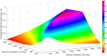
Other additional algorithm refers to optimization of mutual inductance after any of the above-discussed exhaustive procedures are performed and it is referred to as M-Optimizer: Since L x (N x ,Dx ) has an infinite number of possible solutions if no restrictions are imposed, analytical, semi-analytical, and empirical approaches cannot easily indicate the optimized N x or D x for a given target L x that maximizes coupling coefficient k(e,d c ,α) function. In fact, only a computational method is able to perform such a complex combinatory analysis in practical time.
To provide a solution for this problem, an optimization routine was implemented and its objective is to indicate the best coil diameter for emitter and receiver, in a way that k is maximized for a given separation distance e of interest. Basically, any algorithm from I to IV is executed several times for different user-defined N x values (or D x , if it refers to a fixed number of turns situation), but target self-inductances L p and L s are kept the same (notice that it is possible to have L p = L s or L p ≠ L s ). The result is a set of n possible geometrical representations for L p and m possible representations for L s . Notice that each of these representations follow the user-defined restriction (N x or D x ).
Thus, a combinatory analysis is made as follows: First the optimization algorithm creates geometrical entities in blank FEMM files and represent every possible combination of D p and D s (one FEMM file for each combination), making sure that primary and secondary are separated by the user-defined distance. This will result in a number of m times n files. Then, each combination is discretized, simulated, and post-processed. Coupling coefficient is calculated for each possible solution. The raw data are organized in a user-friendly graph, that indicates optimized D p and D s that maximize k (or M).
Figure 7 shows the behavior of mutual inductance (normalized for simplicity) for some possible combinations of D s and D p for a hypothetical coupled system where L p = 3L s /2 at an arbitrary (but fixed) separation distance. If the best D p /Ds ratio is chosen, power transfer may be increased.
Example of M-Optmizer output indicating D p /Ds that maximizes M in color map.

All design algorithms proposed so far are contributions to solve arguments (a) and (c) in the introductory section.
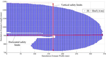
An additional algorithm for TI procedures is H-Mapping: As IPT converters usually make use of frequencies above tens of kHz and currents up to several hundreds of A, it is possible that significant magnetic field intensity |H| result from its operation. Based on [13], which provides limits for general public exposure as a function of f 0, a dedicated routine calculates the maximum reference magnetic field allowed H ref and indicates those spatial coordinates that are in agreement with the safety guidelines. This is done by reading FEMM simulation results point-by-point in Ω 2D .
The resolution of the obtained map depends on FEM mesh size, which is determined automatically according to the materials present in the simulation domain and its dimensions. An example is shown in Fig. 8, where half converter (axisymmetric) was simulated and coordinates where |H| > H ref were hatched in blue.
Example of H-Mapping output indicating regions where magnetic field intensity resulting from the IPT coupler exceeds reference levels defined by [13].

This helps the user to spatially preview and analyze the area under influence of the converter and then add or improve magnetic shields by running the preferred TI algorithm once more. In Fig. 8, the converter (at its maximum excitation parameters) is said to be in accordance with [13] if no general public is present within the area defined by the indicated horizontal and vertical limits.
Through graphical results, this routine provides insights that practitioners need to comprehend basic concepts of safety limits. It should be stated that all the mapping procedure is done solely with implicit design parameters (currents and frequency), which were informed by the user in early stages. Since [13] limits are frequency based, the user does not need to set the safety limits by its own knowledge and inexperienced users can benefit from this tool since they do not require looking up the standard. Experienced users, however, can edit the code to include other safety limits and their own reference levels. This is a contribution to solve argument (b) in the introductory section.
C) TO algorithm
Instead of defining L x,target , one may be interest in designing a IPT system to meet minimum S u , Voc , or I sc or a combination of these parameters. For example, [Reference Nagendra, Covic and Boys6] has minimum S u , Voc , and I sc as target parameter for EV chargers, namely the uncompensated power, secondary open-circuit voltage, and secondary short-circuit current; and [Reference Beh, Covic and Boys14] explicitly must meet minimum S u and V oc .
From the very basic transformer model, with open circuited secondary, (6) is obtained as a function of k, L x , Voc , and primary input voltage V in (which may be expressed as V in,FHA if it refers to the first harmonic approximation). Let L p be user-defined, since it has strong relation with primary resonant circuit, including its operating frequency. Then, V in and V oc are also user inputs, since these parameter are inherent to primary circuit (inverter) characteristics (in the case of V in ) and desired output characteristic (in the case of V oc ). In order to meet a minimum V oc,min , (7) must be achieved.
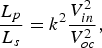 $$\displaystyle{{{L_p}} \over {{L_s}}} = {k^2}\displaystyle{{V_{in}^2} \over {V_{oc}^2}}, $$
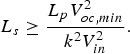 $${L_s} \ge \displaystyle{{{L_p}V_{oc,min}^2} \over {{k^2}V_{in}^2}}. $$
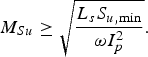
From the output power perspective and considering S u as given by (8) [Reference Elliot, Raabe, Covic and Boys15], (9) must be obeyed to guarantee a minimum S u,min . Notice that (7) and (9) are related by M = k(L p Ls )1/2. Also, k is the unknown and may be actually referred to as a function of geometry/materials of primary and secondary and the relative spatial positioning between them. Anyway, as suggested by [Reference Covic and Boys16], k ≈ 1/Q s,L , where Q s,L is the secondary loaded quality factor, may be used to define a minimum coupling coefficient in order to avoid secondary tuning problems.
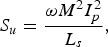 $${S_u} = \displaystyle{{\omega {M^2}I_p^2} \over {{L_s}}},$$
 $${M_{Su}} \ge \sqrt {\displaystyle{{{L_s}{S_{u,\min}}} \over {\omega I_p^2}}}. $$
According to [Reference Nagendra, Covic and Boys6, Reference Elliot, Raabe, Covic and Boys15], S u = V oc Isc , where V oc = jωMI p . I sc can also be determined as shown in (10) with aid of the secondary impedance Z s = R s + jωL s , where R s is the secondary inductor series resistance. Equation (11) must be satisfied to assure I sc,min . Sub-indexes in M Su and M Isc are used to indicate mutual inductance to meet each criterion.
 $${I_{sc}} = \displaystyle{{j\omega M{I_p}} \over {{R_s} + j\omega {L_s}}},$$
 $${M_{Isc}} \ge \left \vert {\displaystyle{{\left( {{R_s} + j\omega {L_s}} \right){I_{sc,min}}} \over {j\omega {I_p}}}} \right \vert. $$
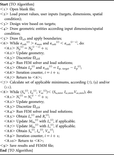
Therefore, considering this formulation, Algorithm V summarizes key steps of TO procedure. Notice that <2> corresponds to user inputs including targets and desired outputs, excitation parameters (ω 0 and I p ), coil shapes (circular, DD, DDQ, and Bipolar) and relative spatial positioning. Loop <6.1> to <6.7> designs primary coil seeking for user-defined L p,target . Differently from what happened in TI algorithms, L p,target is designed under the influence of any magnetic materials existing in the secondary, since the user already defined all material layer thicknesses, type and spatial location in <2>. The same occurs with secondary winding, which is designed in steps <8.1> to <8.10>.
TO algorithm structure.
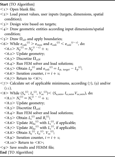
It is worth mentioning that, since primary and secondary are developed in independent loops, each of them can assume any coil shape. Thus, it is possible, as an example, to design a DD primary with a Circular or Bipolar secondary. For this paper, only Circular–Circular is made available since all other shapes are under development or improvement and will be reported in a future opportunity.
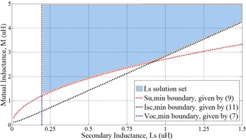
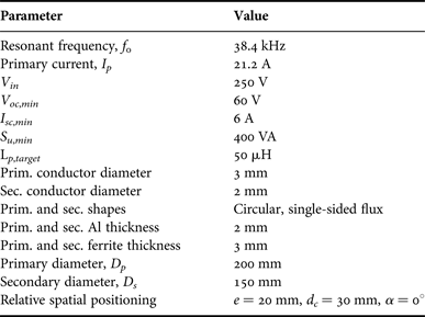
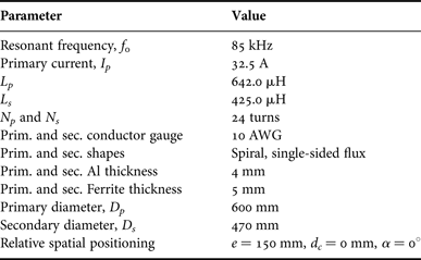
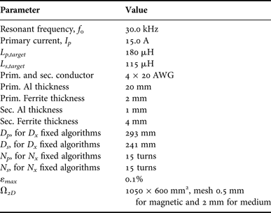
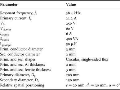
For the hypothetical IPT system described in Table 1, limits to meet V oc , Su , and I sc are graphically demonstrated in Fig. 9. These limits are boundaries that define L s solution set, i.e., values of L s that will meet voltage, current, and power requirements. Note that boundaries (9) and (11) are functions of L s , defined in (7).
Design boundaries to simultaneously guarantee minimum V oc , Su , and I sc for the hypothetical case depicted in Table 1.

Hypothetical IPT system.
One must observe that (8) to (11) express power, voltages, and currents (which are user desires) in terms of frequency, mutual inductance, and self-inductances (which are model entities).
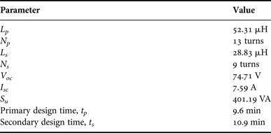
Results obtained after using the TO exhaustive algorithm are shown in Table 2 and required a total time of 21.7 min to achieve a solution. Average iteration time is 44.3 s for primary and 81.8 s for secondary (see Section III for computer specifications), with Ω 2D = 630 × 315 mm2, 2 mm mesh for the medium (air), and 0.5 mm mesh for all coupler materials (copper, aluminum, and ferrite).
TO algorithm results.
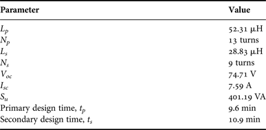
Observing Table 2, one will note that L p differs from L p,target by +4.67%. This is due to the acceptable error ε max in step <6.5> of Algorithm V, which is 5% for this hypothetical case. However, as L p and L s are now defined, user is able to calculate primary and secondary compensation capacitances as described in [Reference Wan, Stielau and Covic17].
Figure 10 shows a cross-section of the final geometry as provided by FEMM at the end of Algorithm V execution (colors and dimensions were added for reference only). This is considered a solution since it simultaneously exceeds V oc,min , I sc,min , and S u,min , as shown in Table 2. The “ball-park” solution can be optimized using aspects discussed in [Reference Beh, Covic and Boys14, Reference Budhia, Covic and Boys18]. Authors of the present work agree with [Reference Nagendra, Covic and Boys6] that optimization typically increase couplers performance to around +20% at most (in terms of uncompensated power, generally). Anyway, depending on coil shape, it may be possible to decrease copper or ferrite usage significantly after some optimization runs. Notice however that optimization is not the purpose of this paper.
Simulated cross-section of a “ball-park” solution that incorporates the results of Table 2.

III. EXPERIMENTAL RESULTS
All simulation times presented in this work were obtained with a very basic and low-cost computer, Intel i3 M380 2.53 GHz processor, 4 GB RAM, in 64 bits operational system, MatLab R2010b running without multi-thread function, or any other special configuration.
A) 2D FEM versus 3D FEM
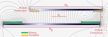
For comparison purposes, a 3D reference design of a coupled system composed by two single-sided flux spiral coils was developed according to Table 3 using 3D FEM solver JMAG Studio. This simulation could not be carried out in the basic specification computer due to several system crashes. Using an Intel i7 processor, 16 GB RAM computer, the time required for a single simulation was 25 min for mesh = 1 mm, and 3D simulation domain Ω 3D = 1800 × 1800 × 1800 mm3.
Parameters of the 3D coupler reference design.
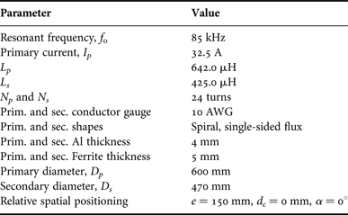
Among the TI algorithms presented, the recommended one for this case is Algorithm III (spiral, fixed N x ). Therefore, with ε max = 0.1% and the same target parameters shown in Table 3 the results are D p = 569.3 mm and D s = 432.8 mm with L p = 641.70 µH, and L s = 425.07 µH.
Note that the TIs were met while coupler diameters differ from the reference 3D design: −5.11% for primary and −7.91% for secondary. This occurs due to: differences in material modeling of both JMAG and FEMM libraries; inherently different solver approaches and boundary conditions necessary in Ω 3D and Ω 2D .
Nevertheless, the 2D design time, including all iterations of the exhaustive algorithm, was 9.9 min for primary and 9.2 min for secondary using the low-cost computer. This clearly shows an advantage of the proposed method. Thus, the solution provided by Algorithm III (and there is no motivation to distrust on the other algorithms) is enough (since errors can be considered small) and fast.
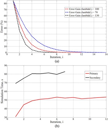
Figure 11(a) shows the ε calc (i) evolution during primary inductor design. Similar curve applies to the secondary. Since ΔD x depends on the error gain λ L , the number of iterations changes accordingly. In general, the higher λ L , the higher ΔD x , and less iterations are required. However, the chance of falling into an unstable and non-converging condition increases.
Parameter evolution during Algorithm III execution, (a) ε calc (i) for different error gains λ L and (b) simulation time for primary and secondary inductors as a function o iteration.

Figure 11(b) shows simulation time as a function of iteration for both primary and secondary. Even though D s < D p , the simulation time for secondary inductor is always higher than for the primary. This occurs because the finite elements of the primary winding (copper) are not being neutralized during the secondary design. Thus, each secondary iteration involves calculating (finite) elements of the highly meshed primary coil. Similarly, note that Figure 11(b) is increasing for both coils. This happens because the magnetic layers (ferrites and Al) increase in size in each iteration, since D x is being increased. Different TI algorithms will present slightly different error and simulation time evolution (as can be inferred from Figs. 3–6 and as discussed in the next section).
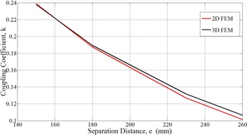
A second 2D versus 3D comparison regards the couplers under misalignment conditions. To perform this comparative study, the 3D reference design was not changed (remain as shown in Table 3) but the 2D design was modified to have the same dimensions of the 3D model (in other words, the cross-section of the 3D model was used in FEMM). Then, the distance between primary and secondary, e, and k(e) was obtained, as shown in Fig. 12. The maximum error between 2D and 3D FEM is −4.78% and occurs when e = 260 mm. Each point simulated in 2D FEM in Fig. 12 has an average run time of 49.4 s, against up to 20 min in 3D FEM.
Simulated k(e) for 2D FEM and 3D FEM.

B) Performance comparison among Algorithms I–IV
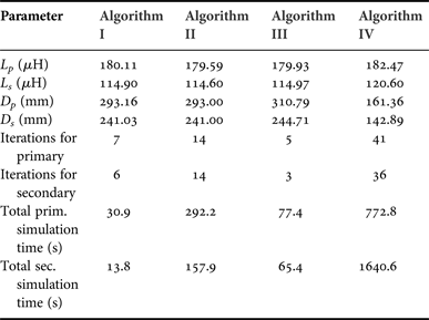
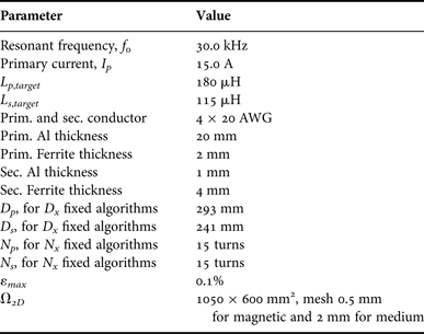
To characterize performance of all four TI algorithms, each of them was executed with parameters shown in Table 4.
Parameters for TI algorithms comparison.
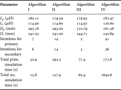
Results, presented in Table 5, demonstrate that all TI algorithms successfully achieve TIs. In terms of simulation time, Algorithms II and IV are considerably slower than the others and this occurs because the number of turns increases from one iteration to the next. Since each turn cross-section is a highly meshed region, it consequently contains high number of finite elements to be solved. Thus, the iteration time increases.
TI algorithms comparison.
One may always keep in mind that each TI algorithm is conceptually different from the others, as each one models a different coupler shape (lumped circular or spiral) or uses a different design variable (N x or D x ).
C) EDAs versus experimental implementation
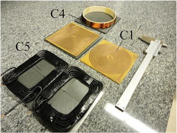
Several coils have been implemented with TI and TO algorithms and tested to perform the comparison of theoretical and experimental results shown in Table 6. Figure 13 illustrate some of the couplers, where magnetic cores are Thornton NB-55/52/4 – TH50. Inductances and series resistances were measured using Philips PM6303 RCL meter.
Designed couplers.

Experimental and simulated results for couplers designed with different exhaustive algorithms.

As one may observe in Table 6, experimental results and design outputs for L x have good agreement. The highest error occurred for C4 coupler. However this geometry is not likely to be used in IPT application due to its high inductance. Interestingly, high series resistance errors were obtained for C4 also. Since C4 has large number of turns (N x = 80) it is possible that the winding modeling error resulted was propagated until a point that it became significant.
Simulation errors are originated intrinsically in the 2D FEM solver, which is a numerical solver that relies in material libraries that may not be fully accurate. Nevertheless, all algorithms performed well, were able to determine physical dimensions of inductors and provided a consistent coupler design.
IV. LIMITATIONS AND OTHER COMMENTS
Since all procedures here presented are based on a 2D FEM solver, all algorithms have an intrinsic limitation which is the impossibility to model geometries that are not planar or axisymmetric. Although simplifying hypothesis can be included if non-axisymmetric or non-planar geometries are to be analyzed, this may result in unreliable results. This limitation exists also when misalignment analysis is performed. For example, in planar representation Ω 2D allows geometrical entities in x and y axis only. All cross-sections defined in Ω 2D , as seen in Fig. 10, must have the same z-dimension (“into the page”) or depth. This is a common source of modeling errors and is a disadvantage of the 2D solver when compared to 3D solver.
Another foreseeable limitation is related to frequency range used in FEMM simulations. Since FEM formulation ignores displacement currents, any EDA must be used if this effect is negligible. There is no indication that EDAs proposed here are limited to a particular dimension range, so couplers can be designed with dimensions from mm to m.
When using the algorithms, one may observe also that the boundary condition applied to Ω 2D is the Prescribed Magnetic Vector Potential ( A boundary = 0, in x and y-directions). This boundary condition is also known as Dirichlet Condition and guarantees that magnetic flux lines do not cross Ω 2D bounds. These bounds must be large enough so that magnetic flux lines originated from the coupler do not become distorted. The algorithms proposed can be modified to include other boundary conditions, but currently the method accuracy and computational time are assured by good empirical mesh-size to Ω 2D -size ratio. Eventually, users willing to have additional performance may find useful to modify meshes and simulation domain dimensions. This can be done easily since all C-codes where implemented in MatLab and are fully commented.
Another relevant comment is about the coil shapes discussed in this paper. As algorithms for Bipolar and other more complex structures were mentioned but not discussed in this paper, the contribution is more directed to circular and spiral coils. This kind of coils, although they are fundamental shapes, are extremely useful for portable electronic equipments such as phones, tablets, and other low-profile devices that may benefit rapidly from IPT. And in terms of popularization of IPT it is more likely that it will begin by simple solutions than by complex geometries. Anyway, the contributions of this paper are general and may fit consumer electronics, biomedical, and EV applications. In addition, all complex couplers are in fact modifications of the circular coil [Reference Budhia, Covic and Boys18–Reference Zhong, Lee and Hui20]. Once one has dominated the design of fundamental coils with shielding layers and spatial positioning analysis, the migration to complex geometries is intuitive and smooth, as the general magnetic concepts are the same.
Finally, after the magnetic coupler has been designed, the power transfer capability of emitter and receiver can be evaluated. At the same time, considering resulting quality factors (predicted with enough confidence by these modeling algorithms), the efficiency of the loosely coupled system can be determined as shown by [Reference Pinuela, Yates, Lucyszyn and Mitcheson21]. Later, if necessary, the designer can extend the efficiency analysis to the converter itself, including performance of high-frequency inverter and resonant networks.
V. CONCLUSIONS
The nature of EDAs is iterative modification of geometric parameters successively updating entities in the simulation domain. Therefore, EDAs provide a connection between electrical variables and physical dimensions. This allows inexperienced designers to have insights on coupler trade-offs and to create a critical sense for future more complex designs. Consequently, one contribution of the EDAs is that they assist and ease knowledge gain (very important feature for IPT popularization), contributing to solve argument (a) from the introductory section.
Inexpensive FEM solver is used in full integration with EDAs and no knowledge on numerical methods is demanded from designers. However, those who wish to modify algorithms and include different convergence techniques, additional calculations (such as magnetic losses) or any kind of artificial intelligence that may improve overall results can easily do so since all algorithms are simple in structure.
In general, TI algorithms (Algorithms I–IV) have the following attributes: Converge to TI in minutes, each iteration taking typically tens of seconds. Convergence time can be optimized if inductance error gain λ L is reduced for Algorithms I and III; Iterations are typically 20 times faster than equivalent 3D FEM simulation. With such reduced simulation time, proposed algorithms are perfectly suitable for home computers (even relying in multiple FEM runs); Experimental results indicate that modeling a coupler in 2D is more conservative than modeling in 3D, since errors are typically negative; Practical implementations also show good results when experimental inductors are compared with designed inductors.
Moreover, since spatial freedom analysis can be obtained by relative axial, lateral, and angular positioning algorithms (which give a full comprehension of the coupler), this paper has contributions to solve argument (c) from the introductory section.
To help solving problems mentioned in argument (b) of Introduction, H-Mapping was developed and does not demand user knowledge to define acceptable magnetic field intensity in the surroundings of a coupler under analysis.
TO algorithms have the same good computational advantages mentioned above and also are able to seek for a magnetic coupler solution that meets minimum output voltage, current, and uncompensated power. An important comment is that user-defined boundaries can be added to Fig. 9, thus limiting even more the set of L s to satisfy minimum requirements. As a simple example, one could define a maximum acceptable value for L s based in the fact that increased inductance leads to larger series resistance, thus affecting Q s , the secondary unloaded quality factor. When more design boundaries are added, the initial or “ball-park” solution becomes closer to an optimized solution.
ACKNOWLEDGEMENTS
Authors would like to express sincere gratitude to Prof. Grant Covic and Prof. John Boys for their support and useful comments on this work during the visit of Mr. Rodolfo Fernandes to the University of Auckland, New Zealand.
 Rodolfo Castanho Fernandes was born in 1986. He graduated in electrical engineering from Univ. Estadual Paulista (UNESP), Ilha Solteira, SP, in 2008. He obtained the MSc. degree in power electronics in 2010 from the same institution. Currently, he is working towards the PhD. degree in dynamical systems at Escola de Engenharia de São Carlos, Universidade de São Paulo. Since 2010 he is with Brazilian heavy automotive industry where he is involved in research and development programs on heavy machinery automation, portable battery operated products and power converters. His research interests include multipulse rectifiers, active power factor correction techniques and wireless power transfer.
 Azauri Albano de Oliveira Jr born in 07/23/1955 in Franca, state of São Paulo, Brazil. He is an electrical and electronic engineer (1977) from the São Carlos Engineering School (EESC) at the University of São Paulo (USP). He has a master’s degree in electrical engineering (1984) from the EESC / USP and a PhD degree in Electrical Engineering (1991) from the Polytechnic School of USP. He is coordinator of the Power Electronics and Control Laboratory (LACEP) of the Electrical and Computer Engineering Department of EESC-USP and professor at the same department since 1978. His areas of interest are: power electronics, drive and control of electrical machines, inductive power transfer, active power filters and electrical engineering education.