1. Introduction
Turbulent Poiseuille flow in a pressure-driven channel between parallel flat plates is the most widely studied case among canonical wall-bounded flows, being an ideal candidate for direct numerical simulation (DNS). Since the pioneering study of Kim, Moin & Moser (Reference Kim, Moin and Moser1987) at low Reynolds number (
 $Re_{{\it\tau}}\approx 180$
, where
 $Re_{{\it\tau}}=h/{\it\delta}_{v}$
, with
 $h$
the channel half-height and
 ${\it\delta}_{v}={\it\nu}/u_{{\it\tau}}$
the viscous length scale), several studies have appeared in which Reynolds numbers are sufficient to observe a nascent logarithmic layer in the mean velocity profile (Moser, Kim & Mansour Reference Moser, Kim and Mansour1999; del Álamo & Jiménez Reference del Álamo and Jiménez2003; Bernardini, Pirozzoli & Orlandi Reference Bernardini, Pirozzoli and Orlandi2014; Lee & Moser Reference Lee and Moser2015). These studies have also allowed the observation of the onset of structural changes in the overall flow organization, mainly related to the strengthening of outer-layer global modes which are found to be superposed onto and modulate the energetic near-wall eddies (Hutchins & Marusic Reference Hutchins and Marusic2007).
At least as important as the statistics of the velocity field are the statistics of passive scalars suspended in the fluid phase, which are representative of the behaviour of diluted contaminants, and/or the temperature field under the assumption of low Mach numbers and small temperature differences (Monin & Yaglom Reference Monin and Yaglom1971; Cebeci & Bradshaw Reference Cebeci and Bradshaw1984). It is well known that measurements of concentrations of passive tracers and of small temperature differences are extremely complicated; in fact available measurements of even basic passive scalar statistics are rather limited (Gowen & Smith Reference Gowen and Smith1967; Kader Reference Kader1981; Subramanian & Antonia Reference Subramanian and Antonia1981; Nagano & Tagawa Reference Nagano and Tagawa1988), mostly including the mean flow properties. Hence, DNS constitutes an invaluable tool for the study of passive scalar turbulence in Poiseuille flow. Early numerical experiments of passive scalars in turbulent channel flow (Kim & Moin Reference Kim and Moin1989) were carried out at
 $Re_{{\it\tau}}=180$
, for
 $Pr=0.1,0.71,2$
(here the molecular Prandtl number is defined as the ratio of the kinematic viscosity to the thermal diffusivity,
 $Pr={\it\nu}/{\it\alpha}$
), by assuming uniform volumetric heating and constant wall properties. That study first showed close similarity in the near-wall region between the streamwise velocity and the scalar fields. Specifically, the scalar field was found to be organized into streaks whose size scales in wall units, with a correlation coefficient between streamwise velocity fluctuations and scalar fluctuations close to one. Numerical studies of scalar fields in a channel driven by differences at the two walls were carried out by Lyons, Hanratty & McLaughlin (Reference Lyons, Hanratty and McLaughlin1991), Wikström & Johansson (Reference Wikström and Johansson1998), Kawamura, Abe & Shingai (Reference Kawamura, Abe, Shingai and Nagano2000). While the behaviour in the near-wall region is similar between the forced case and the assigned scalar difference case, much stronger fluctuations are observed in the latter, owing to the formation of strong core eddies with an organization similar to the velocity field in turbulent Couette flow (Pirozzoli, Bernardini & Orlandi Reference Pirozzoli, Bernardini and Orlandi2014). Furthermore, low-
 $Re$
simulations seemed to suggest influence of the wall state on the Karman constant for the scalar fields (Kawamura et al.
Reference Kawamura, Abe, Shingai and Nagano2000).
Studies of the effect of
 $Pr$
in a wide range have been rather limited so far, mainly because of the need for extremely fine meshes to resolve the scalar fields, since the ratio of the Kolmogorov scale to the Batchelor scalar dissipative scale is supposed to be of the order of
 $Pr^{-1/2}$
(Batchelor Reference Batchelor1959; Tennekes & Lumley Reference Tennekes and Lumley1972). Kawamura et al. (Reference Kawamura, Ohsaka, Abe and Yamamoto1998) performed DNS of channel flow at
 $Re_{{\it\tau}}=180$
with a constant time-averaged heat-flux condition, in the range of Prandtl number
 $0.025\leqslant Pr\leqslant 5$
. The results proved the validity of Kader’s correlation for the passive scalar distribution (Kader Reference Kader1981), and of heat-flux correlations originally developed by Sleicher & Rouse (Reference Sleicher and Rouse1975) for pipe flow. Except for very low
 $Pr$
, the study also showed near universality of the distributions of the turbulent Prandtl number, with values of the order of unity throughout. Schwertfirm & Manhart (Reference Schwertfirm and Manhart2007) extended the study to
 $Pr\approx 50$
, basically observing a continuation of the lower-
 $Pr$
results of Kawamura et al. (Reference Kawamura, Ohsaka, Abe and Yamamoto1998).
Reynolds number effects on passive scalar fields are difficult to study in DNS, owing to the rapid increase of the necessary computational resources. Kawamura, Abe & Matsuo (Reference Kawamura, Abe and Matsuo1999) performed DNS of channel flow with forced scalar fields at
 $Re_{{\it\tau}}=180,395$
, and
 $Pr=0.025,0.2,0.71$
. The main conclusion was that the log-law constant for the scalar field is roughly independent of the Reynolds number, with values of the Karman constant in the range
 $0.40\leqslant k_{{\it\theta}}\leqslant 0.42$
. Similarly, the turbulent Prandtl number was found to be weakly affected by Reynolds number variations. Abe, Kawamura & Matsuo (Reference Abe, Kawamura and Matsuo2004b
) further extended the range of Reynolds numbers to
 $Re_{{\it\tau}}=1020$
, focusing the attention on the variation of the surface heat-flux fluctuations. Those authors estimated a value of the Karman constant of
 $k_{{\it\theta}}\approx 0.43$
, and observed an increase of the r.m.s. wall heat flux with
 $Re_{{\it\tau}}$
, to a greater extent in the case of low
 $Pr$
. Based on the same DNS database, Abe & Antonia (Reference Abe and Antonia2009) quantified the degree of similarity between velocity and scalar fields and their corresponding derivatives near the wall through correlation coefficients, joint p.d.f.s, Taylor series expansions, and instantaneous fields. That study indicated that impaired similarity between streamwise velocity
 $u$
and passive scalars
 ${\it\theta}$
occurs in regions where the magnitude of the streamwise pressure gradient is large due to the presence of near-wall vortical motions. The magnitudes of the scalar–velocity correlation coefficients were found to be relatively unaffected by the Reynolds number, although the authors explicitly stated that a firm conclusion could not be made due to the small range of
 $Re_{{\it\tau}}$
available at that time. Antonia, Abe & Kawamura (Reference Antonia, Abe and Kawamura2009) quantitatively analysed similarities and differences between the fluctuating velocity vector and temperature fluctuations in turbulent channel flow. Strong similarities were observed for the low-wavenumber part of the spectra, whereas the scalar spectra were found to exhibit higher energy at high wavenumbers, especially in the outer region, where the scalar field was found to be less mixed than the velocity field.
The main motivation for the present study is to extend DNS of passive scalars to higher Reynolds numbers, specifically up to
 $Re_{{\it\tau}}\approx 4000$
. It is known (Bernardini et al.
Reference Bernardini, Pirozzoli and Orlandi2014; Lee & Moser Reference Lee and Moser2015) that in this range of Reynolds numbers a near-logarithmic layer starts to emerge in the mean velocity profile; hence asymptotic high-Reynolds-number effects are expected to manifest themselves which were not observed in previous studies.
2. Computational set-up
We solve the Navier–Stokes momentum equations for a divergence-free velocity field
 $$\begin{eqnarray}\frac{\partial u_{j}}{\partial x_{j}}=0,\quad \frac{\partial u_{i}}{\partial t}+\frac{\partial u_{i}u_{j}}{\partial x_{j}}=-\frac{\partial p}{\partial x_{i}}+\frac{1}{Re}\frac{\partial ^{2}u_{i}}{\partial x_{j}\partial x_{j}}+{\it\Pi}{\it\delta}_{i1},\end{eqnarray}$$
where
 ${\it\Pi}$
is the driving force required to maintain a constant flow rate in the
 $x$
direction. The equations are discretized in a Cartesian coordinate system (
 $x,y,z$
denote the streamwise, wall-normal and spanwise directions) using staggered central second-order finite-difference approximations, to guarantee that kinetic energy is globally conserved in the limit of inviscid flow. Time advancement is carried out by means of a hybrid third-order low-storage Runge–Kutta algorithm coupled with the second-order Crank–Nicolson scheme combined in the fractional-step procedure, whereby the convective terms are treated explicitly and the diffusive terms are treated implicitly, limited to the wall-normal direction. The Poisson equation for the pressure field stemming from the incompressibility condition is efficiently solved through Fourier transform-based methods (Kim & Moin Reference Kim and Moin1985). A full description of the algorithm is provided in Orlandi (Reference Orlandi2000). The fluid equations are augmented with the transport equations for passive scalar fields with finite diffusion
 $$\begin{eqnarray}\frac{\partial {\it\theta}}{\partial t}+\frac{\partial {\it\theta}u_{j}}{\partial x_{j}}=\frac{1}{Re\,Pr}\frac{\partial ^{2}{\it\theta}}{\partial x_{j}\partial x_{j}}+Q,\end{eqnarray}$$
where
 ${\it\theta}$
is the transported variable (temperature or concentration),
 $Pr$
is either the Prandtl number or the Schmidt number, and
 $Q$
is a suitable source term. In the numerical discretization the transported variable is located at the cell centre in such a way that the variance of
 ${\it\theta}$
is exactly preserved in the limit of inviscid flow. The source term is defined to be either zero in the case of walls with different values of
 ${\it\theta}$
, or dynamically adjusted in such a way that the integral of
 ${\it\theta}$
over the channel is strictly constant in time, in analogy with the treatment of the driving force in the momentum equation. This approach is slightly different from that used by Kim & Moin (Reference Kim and Moin1989), who also adopted a spatially uniform forcing, however with an a priori selected source term
 $Q=1/Pr$
. Our approach also differs from that used by Kawamura et al. (Reference Kawamura, Ohsaka, Abe and Yamamoto1998) and Abe et al. (Reference Abe, Kawamura and Matsuo2004b
), who enforced a strictly constant wall flux in time by adding a spatially non-uniform source term. In our case, although the wall flux is not strictly constant in time, its value starts to fluctuate with excursions of no more than 1 % with respect to the mean value, once a statistically steady state is achieved. For the sake of efficiency and accuracy (Kleiser & Zang Reference Kleiser and Zang1991; Bernardini et al.
Reference Bernardini, Pirozzoli, Quadrio and Orlandi2013) the computations are carried out in a reference frame in which the bulk velocity is zero. In addition to allowing a larger computational time step, this expedient minimizes the dispersion errors associated with finite-difference discretization.
List of parameters for turbulent channel flow cases.
 $Re_{b}=2hu_{b}/{\it\nu}$
is the bulk Reynolds number and
 $Re_{{\it\tau}}=hu_{{\it\tau}}/{\it\nu}$
is the friction Reynolds number.
 $N_{x}$
,
 $N_{y}$
,
 $N_{z}$
are the number of grid points in the streamwise, wall-normal and spanwise directions, respectively.
 ${\rm\Delta}x^{+}$
,
 ${\rm\Delta}z^{+}$
are the grid spacings in the wall-parallel directions and
 ${\rm\Delta}y_{w}^{+}$
the minimum spacing in the wall-normal direction, in wall units. The simulation time
 $T$
is given in terms of eddy turnover times
 $h/u_{{\it\tau}}$
. An error stretching function
 $y({\it\eta})=\text{erf}[a({\it\eta}-0.5)]/\text{erf}(0.5a)$
,
 $a=4$
,
 ${\it\eta}=[0,1]$
has been used to cluster points in the wall-normal direction.

Details on the computational mesh and on the parameters used for DNS of the fluid phase are provided in table 1. The set-up is very similar to our previous study (Bernardini et al.
Reference Bernardini, Pirozzoli and Orlandi2014), with the main difference of slightly improved resolution in all coordinate directions. The DNS have been carried out in an
 $(L_{x}\times L_{y}\times L_{z})=(6{\rm\pi}h\times 2h\times 2{\rm\pi}h)$
computational box, which is sufficiently long to accommodate the largest outer-layer flow structures. Points are clustered towards the walls according to an error function mapping, to have the first point at
 ${\rm\Delta}y_{w}^{+}\approx 0.1$
, and the maximum spacing in terms of local Kolmogorov units is
 $({\rm\Delta}y/{\it\eta})_{max}\approx 2.4$
for all flow cases. The resolution in the wall-parallel directions in terms of Kolmogorov units is
 ${\rm\Delta}x/{\it\eta}\lesssim 5.3$
,
 ${\rm\Delta}z/{\it\eta}\lesssim 3.6$
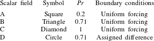
throughout. Since the maximum Prandtl number is unity, Batchelor units (Batchelor Reference Batchelor1959) are larger than or equal to Kolmogorov units, hence the resolution for the scalar fields is no worse than for the velocity field. The adequacy of the mesh resolution has been checked by monitoring the streamwise and spanwise passive scalar spectral densities (not shown here). The absence of any energy pile-up and the exponential decay of the high-wavenumber-end of the spectra is a strong hint that the sharp gradients of passive scalar fields are correctly resolved. A grid sensitivity study has also been performed for the P550 flow case, which has shown that doubling the mesh points in the wall-parallel directions yields a change of less than 1 % in the peak scalar variance. The adequacy of the time interval for the statistical analysis was also tested for the most critical P4000 flow case by comparing the mean and the variance of the passive scalar field, collected in quarters of the full window. The results of this exercise (not shown) indicate scatter of approximately 1 %, confined to the outer wall layer. Four different conditions for the passive scalar fields are considered (see table 2) for each
 $Re_{{\it\tau}}$
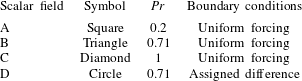
, including three simulations with uniform forcing and
 ${\it\theta}=0$
at the two walls, and one with zero forcing and assigned difference between the two walls (
 ${\it\theta}=\pm 1$
). Of special interest is the case
 $Pr=1$
(scalar field C), which obeys the same equations as the streamwise velocity field, in the absence of nonlinear feedback effects and in the absence of redistribution to the other velocity components through the pressure–strain term (Pope Reference Pope2000).
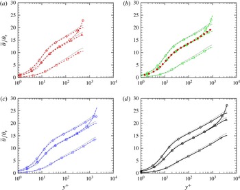
Mean scalar profiles for flow cases P550 (a), P1000 (b), P2000 (c) and P4000 (d). The data are compared with the fits of Kader (Reference Kader1981) (thick grey lines) and with DNS data of Abe et al. (Reference Abe, Kawamura and Matsuo2004b
) at
 $Re_{{\it\tau}}=1020$
(solid symbols in (b)). Refer to tables 1 and 2 for nomenclature of the DNS data.

Test conditions for passive scalar fields.
3. Results
3.1. Mean and r.m.s. values
The mean scalar distributions are given in figure 1 in wall units, where the friction temperature is defined as
 $$\begin{eqnarray}{\it\theta}_{{\it\tau}}=\frac{{\it\alpha}}{u_{{\it\tau}}}\left.\frac{\text{d}\overline{{\it\theta}}}{\text{d}y}\right|_{w},\end{eqnarray}$$
with
 ${\it\alpha}$
being the scalar diffusivity. Semiempirical fits for the mean scalar profiles in channel flows with constant heating were given by Kader (Reference Kader1981) based on available experimental data, under the main assumption that the overlap layer exhibits logarithmic variation of the type
 $$\begin{eqnarray}\frac{\overline{{\it\theta}}-\overline{{\it\theta}}_{w}}{{\it\theta}_{{\it\tau}}}=\frac{1}{k_{{\it\theta}}}\log y^{+}+C_{{\it\theta}}(Pr),\end{eqnarray}$$
where
 $k_{{\it\theta}}$
is the Karman constant for the scalar field, and the additive constant is an empirically determined function of the Prandtl number. The curve fits of Kader (Reference Kader1981) with the original set of constants (including
 $k_{{\it\theta}}=0.47$
) are compared with the DNS data in figure 1. All passive scalar profiles visually exhibit a near-logarithmic layer which is widening with
 $Re_{{\it\tau}}$
and, as well established, the effect of Prandtl number increase is the increase of the additive constant in the logarithmic law, the slope of the graphs being visually the same. The scalar field D with assigned difference at the two walls has a different behaviour than the others, with mean profiles which start to deviate from the corresponding forced case B at
 $y/h\approx 0.2$
and sloping towards the channel centreline where the mean gradient in not zero, similar to the mean velocity profile of Couette flow. This behaviour led Kawamura et al. (Reference Kawamura, Abe, Shingai and Nagano2000) to conclude, based on low-
 $Re$
simulations, that the scalar Karman constant should be different between the forced and assigned temperature case. However, based on the present high-
 $Re$
data we are led to conclude that the mean scalar profile in the logarithmic layer is very little affected by the boundary conditions. Overall good agreement with Kader’s correlation is found, with larger deviations at low Prandtl number. Kader’s formula typically overshoots the numerical values, with deviations up to 4 % in the log layer. Reasons for this difference may reside in the fact that the wall heat flux is not precisely constant in the DNS. The DNS data of Abe et al. (Reference Abe, Kawamura and Matsuo2004b
) at
 $Re_{{\it\tau}}=1020$
,
 $Pr=0.71$
are also shown for comparison in figure 1(b). While the logarithmic part of the profile is very similar to ours, a fuller scalar profile is found in their DNS which better agrees with Kader’s fit. In order to clarify this issue we have carried out additional DNS using the same computational set-up as Abe et al. (Reference Abe, Kawamura and Matsuo2004b
) in terms of box size and/or scalar forcing scheme. Nearly identical results to those of Abe et al. (Reference Abe, Kawamura and Matsuo2004b
) are obtained when the same forcing is used, which suggests that the forcing has an impact on the computed statistics, at least as far as the core part of the channel is concerned.
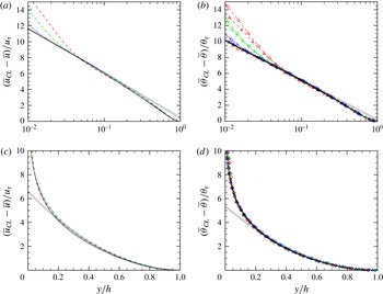
The inner-scaled profiles exhibit clear Prandtl number sensitivity of the scalar fields, owing to a different thickness of the conductive sublayer. To highlight outer scaling, the velocity and scalar profiles are shown in defect form in figure 2. The figure suggests close universality of the profiles with respect to both Reynolds and Prandtl number, in line with theoretical expectations (Monin & Yaglom Reference Monin and Yaglom1971). In the overlap layer, the scalar profiles are nearly logarithmic, with
 $$\begin{eqnarray}\frac{\overline{{\it\theta}}_{CL}-\overline{{\it\theta}}}{{\it\theta}_{{\it\tau}}}=-\frac{1}{k_{{\it\theta}}}\log {\it\eta}+B_{{\it\theta}},\end{eqnarray}$$
where
 ${\it\eta}=y/h$
and
 $\overline{{\it\theta}}_{CL}$
is the mean centreline value. Fitting the DNS data in the defect representation is easier than for the inner-layer representation, and yields an approximate value for the Karman constant for the scalar fields of
 $k_{{\it\theta}}\approx 0.46$
, and an additive constant
 $B_{{\it\theta}}\approx 0.18$
. For comparison, fitting the defect velocity profile (see figure 2
a) yields
 $k\approx 0.41$
,
 $B\approx 0.46$
; hence the wake strength is found to be greater in the velocity field than in the scalar fields.

The shape of the scalar profiles in the core layer of channels have been the subject of several conjectures in the past (Monin & Yaglom Reference Monin and Yaglom1971; Kader Reference Kader1981; Cebeci & Bradshaw Reference Cebeci and Bradshaw1984), which typically led to empirical polynomial fits of the scalar profiles from experimental data. It has been recently shown (Pirozzoli Reference Pirozzoli2014; Orlandi, Bernardini & Pirozzoli Reference Orlandi, Bernardini and Pirozzoli2015) that the crude assumption of uniform eddy viscosity is rather accurate in predicting the mean velocity profiles for all canonical wall-bounded flows, including Poiseuille flow. Specifically, under the assumption that the relevant outer eddy velocity scale is
 $u_{{\it\tau}}$
and the typical size is
 $h$
, one has
 $$\begin{eqnarray}{\it\nu}_{t}=c_{{\it\mu}}u_{{\it\tau}}h,\end{eqnarray}$$
where
 $c_{{\it\mu}}$
is a suitable constant, whence the parabolic core mean velocity law follows
 $$\begin{eqnarray}u_{CL}^{+}-u^{+}=\frac{1}{2c_{{\it\mu}}}(1-{\it\eta})^{2}.\end{eqnarray}$$
We argue that a uniform eddy diffusivity assumption may also apply to passive scalar fields, under the ansatz
 $$\begin{eqnarray}{\it\alpha}_{t}=c_{{\it\alpha}}u_{{\it\tau}}h,\end{eqnarray}$$
which yields the parabolic core scalar law
 $$\begin{eqnarray}{\it\theta}_{CL}^{+}-{\it\theta}^{+}=\frac{1}{2c_{{\it\alpha}}}(1-{\it\eta})^{2}.\end{eqnarray}$$
Fitting (3.7) to the DNS data in figure 2 yields
 $c_{{\it\mu}}\approx 0.076$
,
 $c_{{\it\alpha}}\approx 0.093$
, the relevant turbulent Prandtl number being
 $Pr_{t}={\it\nu}_{t}/{\it\alpha}_{t}\approx 0.81$
. The accuracy of the fit is apparently very good down to
 ${\it\eta}\approx 0.2$
, regardless of the Reynolds and Prandtl number.
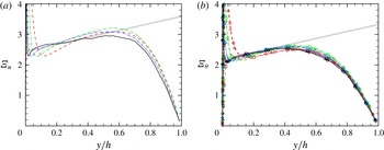
Diagnostic function for mean velocity (a) and for scalar fields A–C (b). The thick grey lines correspond to (3.8) with
 $k=0.41$
,
 ${\it\gamma}=1.1$
,
 ${\it\beta}=0$
(a), and
 $k_{{\it\theta}}=0.46$
,
 ${\it\gamma}_{{\it\theta}}=1.15$
,
 ${\it\beta}_{{\it\theta}}=0$
(b). Refer to tables 1 and 2 for nomenclature of the DNS data.

Although the inner- and outer-scaled scalar profiles appear to exhibit near-logarithmic layers, and the log-layer approximation is in fact satisfactory for most practical purposes, a more into-depth analysis shows that the situation is probably more intricate (Pirozzoli Reference Pirozzoli2014). In figure 3 we show the log-law diagnostic function,
 ${\it\Xi}_{u}=y^{+}\,\text{d}u^{+}/\text{d}y^{+}$
,
 ${\it\Xi}_{{\it\theta}}=y^{+}\,\text{d}{\it\theta}^{+}/\text{d}y^{+}$
, for the velocity and the scalar fields. Clearly, constancy of
 ${\it\Xi}$
would indicate the presence of a genuine log layer. As noticed by Bernardini et al. (Reference Bernardini, Pirozzoli and Orlandi2014), no clear plateau is found in
 ${\it\Xi}_{u}$
, neither for the velocity nor for the scalar field. However, there is rather clear evidence for the presence of a range with nearly linear variation of
 ${\it\Xi}_{u}$
with the wall distance, whose slope (in inner units) decreases with
 $Re_{{\it\tau}}$
, and which is predicted by some refined overlap theories (Afzal & Yajnik Reference Afzal and Yajnik1973). According to such generalized log-layer formulations,
 $$\begin{eqnarray}{\it\Xi}=\frac{1}{k}+{\it\gamma}{\it\eta}+\frac{{\it\beta}}{Re_{{\it\tau}}},\end{eqnarray}$$
where (Bernardini et al.
Reference Bernardini, Pirozzoli and Orlandi2014)
 $k\approx 0.41$
,
 ${\it\gamma}\approx 1.1$
,
 ${\it\beta}\approx 180$
for the streamwise velocity field. Fitting the mean scalar profiles in figure 3(b) in the range
 $100/Re_{{\it\tau}}\leqslant {\it\eta}\leqslant 0.5$
yields
 $k_{{\it\theta}}\approx 0.46$
,
 ${\it\gamma}_{{\it\theta}}\approx 1.15\approx {\it\gamma}$
, with very weak effect of the molecular Prandtl number. It should be noted that the presence of a generalized logarithmic layer does not prevent the onset of a narrow genuine logarithmic layer at higher Reynolds numbers, which however should be confined to a narrower range of wall distances (Lee & Moser Reference Lee and Moser2015).
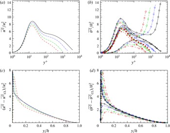
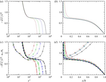
Streamwise velocity variance (a,c) and scalar variance (b,d) as a function of the wall distance in inner units (a,b) and outer units (c,d). In (b) the solid circles indicate the DNS data of Abe et al. (Reference Abe, Kawamura and Matsuo2004b ). Refer to tables 1 and 2 for nomenclature of the DNS data.

The variances of the streamwise velocity and scalar fluctuations are shown in figure 4 in inner and outer scaling. The inner-scaled scalar profiles (b) are strongly affected by the molecular conductivity, being an increasing function of
 $Pr$
. As expected, based on the formal similarity of the governing equations, the shape of the scalar variance profiles at
 $Pr=1$
is similar to the streamwise velocity variance, with the main exception of a higher value of the near-wall peak. Of course, the scalar variance in flow case D has a very different behaviour in the outer layer, where production does not drop to zero (Kawamura et al.
Reference Kawamura, Abe, Shingai and Nagano2000), and a second peak emerges which is larger than the near-wall peak, and also increasing with
 $Re_{{\it\tau}}$
. Comparison with previous DNS by Abe et al. (Reference Abe, Kawamura and Matsuo2004b
) is quite favourable, whereas substantial differences are found with respect to the available experimental data of Subramanian & Antonia (Reference Subramanian and Antonia1981), not shown. The velocity and scalar variances are shown in defect form in (c,d). Collapse in the defect representation is only fair for the velocity field, whereas more convincing universality over the
 $Re$
and
 $Pr$
range is found for the scalar variances. The odd behaviour of the streamwise velocity variance is at the root of alternative (mixed) scalings which have been proposed over the years (DeGraaff & Eaton Reference DeGraaff and Eaton2000; del Álamo et al.
Reference del Álamo, Jiménez, Zandonade and Moser2004), and is probably related to the difficulty in identifying a logarithmic layer as required by the attached-eddy hypothesis (Townsend Reference Townsend1976; Perry & Marusic Reference Perry and Marusic1995; Orlandi et al.
Reference Orlandi, Bernardini and Pirozzoli2015).
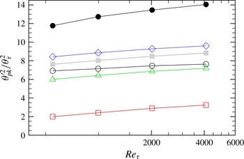
Peak scalar variances at various
 $Pr$
(see table 2 for nomenclature of symbols) as a function of
 $Re_{{\it\tau}}$
, compared with the peak streamwise velocity variance (solid squares). The solid circles denote the centreline peak of the scalar variance for field D.

The peaks of the scalar and streamwise velocity variances are shown in figure 5 as a function of the Reynolds number. Attached-eddy arguments support a logarithmic increase of the inner peak of the streamwise velocity variance with
 $Re_{{\it\tau}}$
because of the increasing effect of overlying attached eddies (Townsend Reference Townsend1976; Hutchins et al.
Reference Hutchins, Nickels, Marusic and Chong2009). The present data suggest that the same behaviour also applies to passive scalar fields. Specifically, we find that the growth rate is approximately the same at all
 $Pr$
, with a strongly increasing additive constant. The case of assigned wall difference shows a moderate increase in the near-wall peak for given
 $Pr$
, owing to energy leakage from stronger eddies forming in the channel core (also see the later spectral maps). As previously noticed, scalar field D also exhibits a prominent peak at the channel centreline, whose amplitude (solid circles in figure 5) shows a similar growth rate with
 $Re_{{\it\tau}}$
as the near-wall peaks.


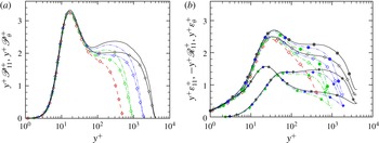
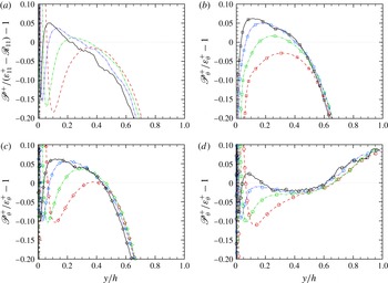
Premultiplied production (a) and dissipation rate (b) of streamwise velocity field (lines) and passive scalar field C (lines
 $+$
open symbols). The solid symbols in (b) denote the contributions of viscous dissipation
 ${\it\varepsilon}_{11}$
(squares) and pressure
 $\mathscr{R}_{11}$
(diamonds), and their sum (circles). Refer to table 1 for the line style.

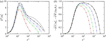
Similarities between passive scalar and streamwise velocity statistics are more closely scrutinized in figure 6, where we compare the variances and the vertical turbulent fluxes for
 $Pr=1$
(scalar field C). As previously noticed, the scalar variances attain a higher peak in the near-wall region, whereas they tend to form log-like layers for
 $100/Re_{{\it\tau}}\leqslant {\it\eta}\leqslant 0.2$
. In this region the streamwise velocity variance is higher and tends to form a ‘bump’ which precludes the observation of a logarithmic layer, although no evidence for an outer peak is found at the Reynolds numbers under scrutiny. On the other hand, the vertical turbulent fluxes, shown in figure 6(b), are (visually) very nearly indistinguishable, hence suggesting that the lift-up mechanism which is responsible for the
 $u{-}v$
and
 $v{-}{\it\theta}$
correlations is very nearly linear in nature. At the same time, it must be stated that small differences in the vertical turbulent fluxes are at the core of observable differences in the mean profiles, which were clear in figure 1.
3.2. Energetics
Differences in the behaviour of scalar and streamwise velocity variances can be further elaborated by monitoring the respective budget equations, reported below (Pope Reference Pope2000)
 $$\begin{eqnarray}\displaystyle & \displaystyle 0=-\frac{\text{d}\overline{v^{\prime }u^{\prime 2}/2}}{\text{d}y}+{\it\nu}\frac{\text{d}^{2}\overline{u^{\prime 2}/2}}{\text{d}y^{2}}\underbrace{-\,\overline{u^{\prime }v^{\prime }}\frac{\text{d}\overline{u}}{\text{d}y}}_{\mathscr{P}_{11}}-\,\frac{\text{d}\overline{p^{\prime }v^{\prime }}}{\text{d}y}+\underbrace{\overline{p^{\prime }\frac{\partial u^{\prime }}{\partial x}}}_{\mathscr{R}_{11}}-\underbrace{{\it\nu}\overline{\frac{\partial u^{\prime }}{\partial x_{k}}\frac{\partial u^{\prime }}{\partial x_{k}}}}_{{\it\varepsilon}_{11}}, & \displaystyle\end{eqnarray}$$
 $$\begin{eqnarray}\displaystyle & \displaystyle 0=-\frac{\text{d}\overline{v^{\prime }{\it\theta}^{\prime 2}/2}}{\text{d}y}+{\it\alpha}\frac{\text{d}^{2}\overline{{\it\theta}^{\prime 2}/2}}{\text{d}y^{2}}\underbrace{-\,\overline{{\it\theta}^{\prime }v^{\prime }}\frac{\partial \overline{{\it\theta}}}{\partial y}}_{\mathscr{P}_{{\it\theta}}}-\underbrace{{\it\alpha}\overline{\frac{\partial {\it\theta}^{\prime }}{\partial x_{k}}\frac{\partial {\it\theta}^{\prime }}{\partial x_{k}}}}_{{\it\varepsilon}_{{\it\theta}}}. & \displaystyle\end{eqnarray}$$
In figure 7 we show the source terms in (3.9), (3.10) associated with production (
 $\mathscr{P}_{11}$
and
 $\mathscr{P}_{{\it\theta}}$
, respectively), viscous dissipation (
 ${\it\varepsilon}_{11}$
and
 ${\it\varepsilon}_{{\it\theta}}$
), and pressure–strain correlation (
 $\mathscr{R}_{11}$
, absent in the scalar variance equation). It must be noted that, in order to more closely compare small terms (all scaling as
 $1/y$
), the various quantities are reported in premultiplied form in a semilog representation, so that equal areas underneath the curves correspond to equal integral contributions. The near-wall region (say
 $y^{+}\lesssim 100$
) is characterized by nearly equal values of velocity and scalar production. On the other hand, similarity of velocity and scalar dissipation is confined to the viscous sublayer, consistent with the analogy noticed by Abe & Antonia (Reference Abe and Antonia2009). Further away from the wall the dissipation rates become very different, the velocity dissipation being much less than the scalar dissipation. However, this difference is more than compensated by the pressure term in the streamwise momentum equation, which should hence be regarded as responsible for the lower near-wall peak of the velocity variance as compared to the scalar variance. In the outer wall layer, streamwise momentum production significantly exceeds scalar production, thus making up for the previously noticed outer bump in the streamwise velocity variance. Consistent with greater production, the total velocity dissipation is also found to exceed scalar dissipation, mostly because of the pressure term, whose premultiplied distribution tends to form an outer peak.
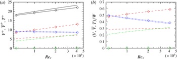
Global energy balance of streamwise velocity (lines) and scalar field C (lines and symbols) as a function of Reynolds number, expressed in wall units (a) and as a fraction of the total power expenditure (b). Solid lines: total power expenditure (
 $W$
); dashed lines: turbulent dissipation (
 $V$
); dash-dot-dotted lines: mean flow dissipation (
 $\overline{V}$
); dash-dotted lines: pressure transfer (
 $T$
).

The effect of the various source terms in the variance budgets can be appreciated by inspecting the global energy balance equations, which are easily derived from the streamwise momentum and scalar transport equations
 $$\begin{eqnarray}\displaystyle & \displaystyle \underbrace{h{\it\Pi}u_{b}}_{W}=\underbrace{\int _{0}^{h}{\it\varepsilon}_{11}\,\text{d}y}_{V_{11}}+\underbrace{\int _{0}^{h}-\mathscr{R}_{11}\,\text{d}y}_{T}+\underbrace{{\it\nu}\int _{0}^{h}(\text{d}\overline{u}/\text{d}y)^{2}\,\text{d}y}_{\overline{V}_{11}}, & \displaystyle\end{eqnarray}$$
 $$\begin{eqnarray}\displaystyle & \displaystyle \underbrace{hQ{\it\theta}^{\ast }}_{W_{{\it\theta}}}=\underbrace{\int _{0}^{h}{\it\varepsilon}_{{\it\theta}}\,\text{d}y}_{V_{{\it\theta}}}+\underbrace{{\it\alpha}\int _{0}^{h}(\text{d}\overline{{\it\theta}}/\text{d}y)^{2}\,\text{d}y}_{\overline{V}_{{\it\theta}}}, & \displaystyle\end{eqnarray}$$
where
 ${\it\theta}^{\ast }=1/h\int _{0}^{h}\overline{{\it\theta}}\,\text{d}y$
is the mean value of
 ${\it\theta}$
across the channel, which states that the power spent to force the momentum and the scalar transport equations is partly dissipated by the mean flow (the
 $\overline{V}$
terms) and by turbulent motions (the
 $V$
terms), and partly to produce the wall-normal and spanwise velocity components (the
 $T$
redistributive term). The budget terms of (3.11) and (3.12) are shown in figure 8, in wall units (a) and as a fractional contribution to the overall power expenditure (b). As expected, the power expenditure (
 $W$
) in wall units (which reduces to
 $W^{+}=u_{b}^{+}=\sqrt{2/C_{f}}\sim \log Re_{{\it\tau}}$
in the streamwise momentum equation, where
 $C_{f}$
is the wall friction coefficient) is increasing logarithmically with
 $Re_{{\it\tau}}$
, both for the velocity and for the scalar field, although slightly faster growth is found for the former. In the scalar field, the growth is clearly associated with growth of the turbulent dissipation term, whereas mean flow dissipation is very weakly decreasing with
 $Re_{{\it\tau}}$
. In the streamwise velocity field, mean flow dissipation is again nearly constant, but both turbulent dissipation and pressure redistribution are increasing with
 $Re_{{\it\tau}}$
. As clearer in (b), the latter term is increasing faster, and it is expected to dominate in the asymptotic high-
 $Re$
regime, if the slow logarithmic trends here observed are confirmed.

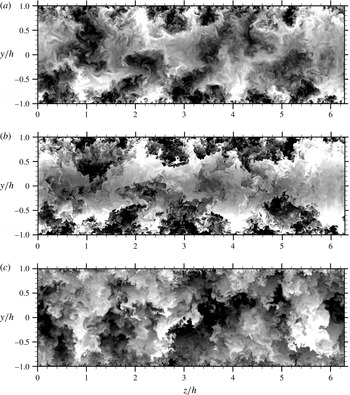
Instantaneous cross-stream visualizations of
 $u^{\prime }$
(a), and
 ${\it\theta}^{\prime }$
for scalar field C (b) and D (c), for flow case P4000. (a) From
 $-3u_{{\it\tau}}$
to
 $3u_{{\it\tau}}$
; (b) from
 $-2{\it\theta}_{{\it\tau}}$
to
 $2{\it\theta}_{{\it\tau}}$
; (c) from
 $-4{\it\theta}_{{\it\tau}}$
to
 $4{\it\theta}_{{\it\tau}}$
. Sixty-four contour levels are shown, in shades from black to white.

The production excess over the total dissipation is displayed in figure 9. It appears that a production excess of up to approximately 5 % is present from
 $y^{+}\approx 200$
to
 $y/h\approx 0.5$
in the velocity field and in the scalar fields with uniform forcing. On the other hand, scalar field D with assigned wall difference has excess production in the core of the channel, say
 $y/h\gtrsim 0.6$
, where the large eddies reside. It is noteworthy that, in the outer representation, the production excess curves attain a common outer envelope which, if extrapolated, would probably lead to a finite value in the infinite-Reynolds-number limit. This outer-layer production excess has been previously linked to the presence of large energy-containing eddies in Poiseuille flow (Bernardini et al.
Reference Bernardini, Pirozzoli and Orlandi2014), and it is more apparent in Couette flow (Pirozzoli et al.
Reference Pirozzoli, Bernardini and Orlandi2014). This is confirmed by the flow visualizations of figure 10, where we report instantaneous cross-stream contours of
 $u^{\prime }$
and
 ${\it\theta}^{\prime }$
(for scalar fields C and D), for flow case P4000, taken at the same time instant. The velocity field and the scalar field in the forced case away from walls is organized into ‘towering’ eddies, which are attached to the wall and exhibit spanwise growth with the wall distance. Particularly striking is the similarity between the streamwise velocity fluctuation field and the passive scalar field C, which clearly indicates that eddies supporting momentum fluctuations also carry the scalar field. In this respect it should also be noted that the interfaces between neighbouring eddies are visually sharper in the scalar field, whereas they are more ‘blurred’ in the velocity field, which is a likely consequence of its active behaviour. Similar observations at lower Reynolds number were reported by Antonia et al. (Reference Antonia, Abe and Kawamura2009). Also striking is the similarity between the two scalar fields in the lower part of the channel (say
 $y/h\lesssim 0.5$
), where the correlation coefficient (not shown) is always larger than 0.8. However, a different organization is recovered in the channel core, where scalar field D exhibits very large eddies, reminiscent of the momentum eddies in Couette flow (Pirozzoli et al.
Reference Pirozzoli, Bernardini and Orlandi2014).
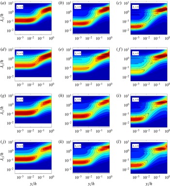
Variation of premultiplied, normalized spanwise spectral densities with wall distance: (a–c) spectra of
 $u$
(
 $k_{z}\hat{E}_{u}$
) for flow cases P1000 (a), P2000 (b), P4000 (c); (d–l) spectra of
 ${\it\theta}$
(
 $k_{z}\hat{E}_{{\it\theta}}$
) for flow cases P1000 (d,g,j), P2000 (e,h,k), P4000 (f,i,l), for the scalar fields A (d–f), C (g–i), D (j–l). Contour levels from 0 to 0.5 are shown, in intervals of 0.04.

This scenario is quantitatively confirmed by the spectral maps shown in figure 11. In order to highlight scale changes, in the figure we show the spanwise spectral densities of the streamwise velocity and of the scalar fields, normalized by the respective variance, by defining
 $$\begin{eqnarray}\hat{E}_{{\it\varphi}}(k_{z})=E_{{\it\varphi}}(k_{z})/\overline{{\it\varphi}^{\prime 2}}.\end{eqnarray}$$
The maps clearly bring out a two-scale organization of the flow field, with a near-wall peak associated with the wall regeneration cycle (Jiménez & Pinelli Reference Jiménez and Pinelli1999), and an outer peak associated with outer-layer large-scale motions (Hutchins & Marusic Reference Hutchins and Marusic2007). The latter peak is found to be centred at
 $y/h\approx 0.3$
, and to correspond to eddies with typical wavelength
 ${\it\lambda}_{z}/h\approx 1$
, consistent with the findings of Abe, Kawamura & Choi (Reference Abe, Kawamura and Choi2004a
). Secondary peaks corresponding to harmonics of this fundamental wavelength are observed at the higher Reynolds numbers, suggesting that the typical outer modes are not purely sinusoidal with respect to the spanwise direction. Notably, the same organization is recovered in the scalar fields. While the near-wall peak depends sensitively in magnitude (but not position and wavelength) on the Prandtl number, being inhibited by diffusion at low
 $Pr$
, the outer peak is quite robust and universal with respect to both
 $Re$
and
 $Pr$
. The main effect of passive scalar forcing is the presence of extra energy near the channel centreline, associated with the large core eddies of figure 10(c).
The structure of the flow field and the statistical association between velocity and scalar fluctuations can be further analysed in terms of the correlation coefficients, defined as
 $$\begin{eqnarray}C_{ab}=\frac{\overline{a^{\prime }b^{\prime }}}{(\overline{a^{\prime 2}}\,\overline{b^{\prime 2}})^{1/2}},\end{eqnarray}$$
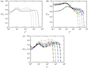
and shown in figure 12. As also previously noticed by Priyadarshana & Klewicki (Reference Priyadarshana and Klewicki2004), the
 $u{-}v$
correlation coefficient stays close to 0.4 throughout the wall layer, with a slight but steady reduction as
 $Re_{{\it\tau}}$
increases, which may be interpreted as a reduction in the flow anisotropy. What we see here is that the
 $v{-}{\it\theta}$
correlation exhibits a similar trend with respect to the Reynolds number, and it also appears to be an increasing function of
 $Pr$
. The
 $u{-}{\it\theta}$
correlation coefficients further highlights strong correlation of streamwise velocity and scalar fluctuations, as also found in previous dedicated studies (Antonia et al.
Reference Antonia, Abe and Kawamura2009). The main finding here is that, while the values in the outer layer seem to be similar for all the flow cases, the near-wall correlation is diminished in the low-
 $Pr$
cases, as the diffusion rate for momentum and scalar fields is sensibly different (Kawamura, Abe & Matsuo Reference Kawamura, Abe and Matsuo2004).


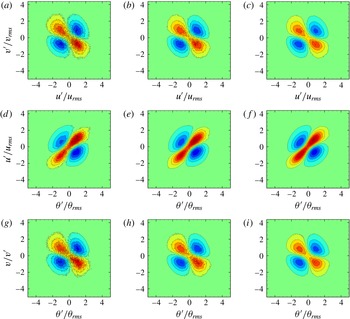
‘Coherent’ part of joint p.d.f.s at
 $y^{+}=5$
, for flow case P1000 (a,d,g), P2000 (b,e,h), P4000 (c,f,i), scalar field C. Sixteen contour levels are shown, from
 $-0.04$
to 0.04 in (a–c), (g–i) and from
 $-0.36$
to 0.36 in (d–f). Colour scale is from blue (negative values) to red (positive values).

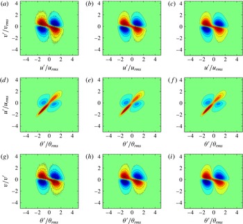
‘Coherent’ part of joint p.d.f.s at
 $y^{+}=100$
, for flow case P1000 (a,d,g), P2000 (b,e,h), P4000 (c,f,i), scalar field C. Sixteen contour levels are shown, from
 $-0.04$
to 0.04 in (a–c), (g–i), and from
 $-0.1$
to 0.1 in (d–f). Colour scale is from blue (negative values) to red (positive values).

Additional details can be captured by analysing the joint p.d.f. of the normalized velocity and scalar fluctuations. Let
 $\tilde{a}=a^{\prime }/\overline{a^{\prime 2}}^{1/2}$
be a normalized fluctuation of variable
 $a$
, the correlation coefficient between
 $a$
and
 $b$
is
 $$\begin{eqnarray}C_{ab}=\iint \tilde{a}\tilde{b}\,P(\tilde{a},\tilde{b})\,\text{d}\tilde{a}\,\text{d}\tilde{b}.\end{eqnarray}$$
We then define the ‘coherent’ part of the joint p.d.f. of
 $a$
and
 $b$
as
 $$\begin{eqnarray}P^{\prime }(\tilde{a},\tilde{b})=P(\tilde{a},\tilde{b})-P(\tilde{a})\cdot P(\tilde{b}),\end{eqnarray}$$
in such a way that it is identically zero if
 $a$
and
 $b$
are statistically independent. The joint p.d.f.s thus constructed then convey information about the local ‘excess’ or ‘lack’ of events with respect to the case of statistical independence, and of course their integrated value is zero, rather than unity. It is also straightforward to show that
 $$\begin{eqnarray}C_{ab}=\iint \tilde{a}\tilde{b}\,P^{\prime }(\tilde{a},\tilde{b})\,\text{d}\tilde{a}\,\text{d}\tilde{b}.\end{eqnarray}$$
In figures 13 and 14 we show the coherent joint p.d.f.s of velocity and scalar fluctuations at various
 $Re_{{\it\tau}}$
, at
 $y^{+}=5$
and
 $y^{+}=100$
, limited to
 $Pr=1$
(scalar field C). At
 $y^{+}=100$
, the
 $u{-}v$
and
 $v{-}{\it\theta}$
joint p.d.f.s indicate increased frequency of events in the second and fourth quadrant, with maxima at approximately one standard deviation from the mean. On the other hand, the
 $u{-}{\it\theta}$
joint p.d.f.s show a clear preference for events in the first and third quadrant, again with maximum values approximately one standard deviation away from the mean. A similar behaviour is also recovered near the wall, where events in the
 $u{-}{\it\theta}$
plane are even more concentrated along the main diagonal, whereas events with low absolute value of
 $v^{\prime }$
seem to be favoured in the
 $u{-}v$
and
 $v{-}{\it\theta}$
joint p.d.f.s. The p.d.f.s here reported do not show visually observable hints of Reynolds number dependence.
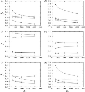
Quadrant contributions to correlation coefficients of
 $u{-}v$
(a,b),
 $u{-}{\it\theta}$
(c,d),
 $v{-}{\it\theta}$
(e,f) at
 $y^{+}=5$
(a,c,e) and
 $y^{+}=100$
(b,d,f), for scalar field C. Quadrant I: squares; quadrant II: triangles; quadrant III: diamonds; quadrant IV: circles.

To identify the motions responsible for the previously noticed Reynolds number variation of the correlation coefficients, in figure 15 we show the quadrant contributions to (3.17) in such a way that they add up to the correlation coefficient. The
 $u{-}v$
correlation (a,b) receives positive contributions from all quadrants (unlike in the conventional quadrant analysis), with a greater influence of the second-quadrant motions (ejections), which are apparently responsible for the decreasing trend with
 $Re_{{\it\tau}}$
. On the other hand, fourth-quadrant motions (sweeps) seem to be marginally affected. A very similar scenario is observed for the
 $v{-}{\it\theta}$
correlation in (e,f). The quadrant contributions to the
 $u{-}{\it\theta}$
correlations, shown in (c,d), highlight the dominant contributions from first- and especially third-quadrant events, namely events with like-signed
 $u$
and
 ${\it\theta}$
fluctuations, and insensitivity to
 $Re_{{\it\tau}}$
.

It is noteworthy that the observed changes in the
 $u{-}v$
and
 $v{-}{\it\theta}$
correlation coefficients can be effectively compensated through normalization with the respective wall-normal velocity variance, as shown in figure 16. Compared with figure 12, it shows near universality of
 $-\overline{u^{\prime }v^{\prime }}/\overline{v^{\prime 2}}$
, both in the inner and in the outer layer, with an overlap layer extending from
 $y^{+}\approx 100$
to
 $y/h\approx 0.5$
, in which the distribution is then expected to be logarithmic (as in fact it probably is), with values not far from 0.7. Concerning the scalar fields, the figures again show universality with
 $Re$
in the inner and in the outer layer, the effect of
 $Pr$
being limited to the conductive sublayer. In the overlap layer a logarithmic distribution is clearly established for the cases with uniform forcing, with values close to those of the turbulent shear stress. The similarity between turbulent fluxes and vertical velocity fluctuations is probably not unexpected, since the production term in the evolution equation for the turbulent shear stress is proportional to the vertical velocity variance (Pope Reference Pope2000). The same can be readily shown also for the vertical turbulent scalar flux. Constancy of the
 $u{-}v$
and
 $v{-}{\it\theta}$
correlation coefficients, which is at the core of many classical turbulence models (i.e. the
 $k{-}{\it\varepsilon}$
model), is put into question by the present DNS results, hence the above information is potentially useful for the construction of improved models for turbulent scalar transport, for instance in the fashion of Durbin’s
 $k{-}{\it\varepsilon}{-}v^{2}$
model (Durbin Reference Durbin1991).
3.3. Engineering correlations
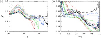
A quantity of great importance in Reynolds-averaged Navier–Stokes (RANS) models of scalar transport is the turbulent Prandtl number, defined as (Cebeci & Bradshaw Reference Cebeci and Bradshaw1984)
 $$\begin{eqnarray}Pr_{t}=\frac{{\it\nu}_{t}}{{\it\alpha}_{t}}=\frac{\overline{u^{\prime }v^{\prime }}}{\overline{v^{\prime }{\it\theta}^{\prime }}}\frac{\text{d}\overline{{\it\theta}}/\text{d}y}{\text{d}\overline{u}/\text{d}y},\end{eqnarray}$$
whose distribution is shown in figure 17. Consistent with most available numerical and experimental data (Kader Reference Kader1981; Cebeci & Bradshaw Reference Cebeci and Bradshaw1984), for
 $Pr\approx 1$
,
 $Pr_{t}$
is not far from
 $0.85$
in a large part of the wall layer, from
 $y^{+}\approx 100$
to
 $y/h\approx 0.5$
. Deviations appear in case A at
 $Pr=0.2$
, for which
 $Pr_{t}$
is closer to
 $0.9$
. Unlike previous simulations at lower
 $Re$
(Kawamura et al.
Reference Kawamura, Abe, Shingai and Nagano2000), the turbulent Prandtl number is not found to be severely affected by the wall state, at least far from the channel centreline. Theoretical estimates for the wall-normal variation of
 $Pr_{t}$
in the inner layer were proposed by Cebeci (Reference Cebeci1973), according to which
 $$\begin{eqnarray}Pr_{t}=\frac{k}{k_{{\it\theta}}}\frac{1-\exp (-y^{+}/A)}{1-\exp (-y^{+}/B)},\quad B=\frac{1}{Pr^{1/2}}\mathop{\sum }_{i=1}^{5}C_{i}(\log _{10}Pr)^{i-1},\end{eqnarray}$$
where
 $A=26$
,
 $C_{1}=34.96$
,
 $C_{2}=28.79$
,
 $C_{3}=33.95$
,
 $C_{4}=6.3$
,
 $C_{5}=-1.186$
. The predictions of (3.19), shown in grey lines in figure 17, are found not to be very accurate. It is also noteworthy that the assumption of constant
 $Pr_{t}$
is not very accurate in the central part of the channel, where the distributions fall rather abruptly to lower values, consistent with the observations previously made about figure 2.


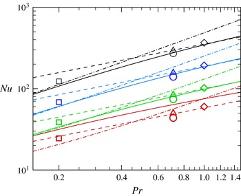
Nusselt number for scalar fields A–D (symbols as in table 2) at various Reynolds numbers (colours as in table 1), compared with the empirical formulae of Kays, Crawford & Weigand (Reference Kays, Crawford and Weigand1980) (dashed lines), Sleicher & Rouse (Reference Sleicher and Rouse1975) (dot-dashed lines) and Gnielinski (Reference Gnielinski1976) (solid lines).

Another quantity of primary engineering interest is the Nusselt number, defined as
 $$\begin{eqnarray}Nu=\frac{h}{({\it\theta}_{b}-{\it\theta}_{w})}\left.\frac{\text{d}\overline{{\it\theta}}}{\text{d}y}\right|_{w},\end{eqnarray}$$
where
 ${\it\theta}_{b}=\int u{\it\theta}\,\text{d}y/\!\int u\,\text{d}y$
is the bulk value of
 ${\it\theta}$
, which is shown in figure 18. As is well known (Cebeci & Bradshaw Reference Cebeci and Bradshaw1984),
 $Nu$
is found to be an increasing function of the Reynolds and the Prandtl number. It is noteworthy that scalar field D, which corresponds to the case of assigned temperature difference, yields very similar (in fact, slightly smaller) Nusselt number than case B with uniform heating. In fact, it turns out that although the heat flux is larger in case D owing to more efficient redistribution of temperature in the core part of the channel by the previously noticed large eddies, the bulk temperature is also larger, the two effects very nearly compensating each other in (3.20). In the figure we also report predictions from the empirical fits for constant temperature walls proposed by Kays et al. (Reference Kays, Crawford and Weigand1980)
 $$\begin{eqnarray}Nu=0.021Re_{b}^{0.8}\,Pr^{0.5},\end{eqnarray}$$
by Sleicher & Rouse (Reference Sleicher and Rouse1975),
 $$\begin{eqnarray}Nu=4.8+0.0156Re_{b}^{0.85}\,Pr^{0.93},\end{eqnarray}$$
as well as the thermal analogy by Gnielinski (Reference Gnielinski1976)
 $$\begin{eqnarray}Nu=\frac{PrC_{f}/2(Re_{b}-1000)}{1+12.7(C_{f}/2)^{1/2}(Pr^{2/3}-1)},\end{eqnarray}$$
where
 $C_{f}$
is the skin friction coefficient. Figure 18 shows accurate prediction of Kays and Crawford correlation at
 $O(1)$
Prandtl number, and superior accuracy of the formula by Sleicher–Rouse at low
 $Pr$
. Gnielinski’s thermal analogy performs relatively well at all
 $Pr$
under scrutiny, and it can probably be further improved by slightly changing the additive coefficient in the numerator of (3.23). Consistent with the previous observations, the above correlations can be applied with the same accuracy to both the case of assigned wall temperature difference and assigned heat flux.
4. Conclusions
The statistics of passive scalars in turbulent channel flow have been studied by means of DNS at much higher Reynolds number than previous studies, and some previously unnoticed features have been brought to light. Upon visual analysis, the mean scalar profiles are found to qualitatively agree with semiempirical models (Kader Reference Kader1981) based on logarithmic overlap layer behaviour with a Prandtl-dependent shift. However, closer examination shows that, similar to what previously found for the velocity field (Bernardini et al.
Reference Bernardini, Pirozzoli and Orlandi2014), the scalar fields also exhibit systematic deviations from the logarithmic behaviour, mainly in the form of an additional term scaling linearly with the outer wall distance, whose slope thus decreases with
 $Re_{{\it\tau}}$
in wall units. This ‘extended’ logarithmic layer occupies approximately 50 % of each half-channel, hence it is much wider than alleged ‘genuine’ log layers which may arise at yet higher Reynolds number. The outer representation is particularly useful in this respect as it allows one to identify, with good approximation, asymptotic values of the Karman constant, which is found to be
 $k=0.41$
for the velocity field, and
 $k_{{\it\theta}}=0.46$
for the scalar field, regardless of the Prandtl number and of the wall state. The outer defect representation also clearly highlights the presence of extended regions with parabolic variation of the mean scalar fields and of the velocity field in the core of forced channels, which smoothly join the quasilogarithmic overlap profiles. It is found that the curvature of the parabolic region is higher for the velocity field, hence making up for a stronger wake region with respect to passive scalars. This observation has been traced to greater eddy diffusivity of the scalar field, which is reflected in a turbulent Prandtl number below unity throughout the outer layer (say,
 $y^{+}\gtrsim 100$
). The scalar variance fields are found to have the same qualitative behaviour as the streamwise velocity variance, with the exception of the case of assigned wall difference, which also exhibits significant scalar activity towards the channel centreline. The near-wall peak in the buffer layer is inhibited at low Prandtl number, as the thickness of the conductive sublayer is comparable to the buffer layer thickness. The amplitude of the near-wall scalar variance peak at
 $Pr=1$
appears to be higher than for the streamwise velocity field, as in the latter case redistributive effects due to pressure/strain correlation are activated. A near-logarithmic layer appears away from the wall, followed by a nearly universal core region, where the scalar variances are again near parabolic. In this region the turbulence kinetic energy production term is larger than the scalar production term, hence the streamwise velocity fluctuations are stronger than the scalar fluctuations, which is the likely reason why a ‘bump’ is observed in the velocity variances rather than a genuine logarithmic layer, at least at these Reynolds numbers. Throughout the wall layer the scalar dissipation is found to be significantly larger than the streamwise velocity dissipation, which implies that the smallest scalar-bearing eddies are more energetic, as confirmed by inspection of their energy spectra. This is also reflected in the instantaneous flow visualizations, which show sharper fronts of the scalar-bearing eddies as compared to those associated with the streamwise velocity field, although visual correspondence of the two fields is clear, and their correlation coefficient remains higher than 0.6 across a large part of the wall layer. Reynolds number effects manifest themselves in the decrease of the
 $u{-}v$
and
 $u{-}{\it\theta}$
correlation coefficients in the outer layer, which is an indication that inactive motions become comparatively more important. An in-depth analysis has shown that the decrease is mainly related to a decreased contribution of the second-quadrant motions (ejections), and it can be compensated by normalization with the vertical velocity variance. From an engineering standpoint, our high-
 $Re$
data show that the turbulent Prandtl number remains in the range between 0.85 and 0.9 in the lower 50 % of the wall layer, and it decreases almost linearly towards the centreline, where
 $Pr_{t}\approx 0.7$
. The Nusselt number follows the classical increasing behaviour with
 $Re_{{\it\tau}}$
and
 $Pr$
, and it is in good agreement with established thermal analogies. Open issues include the detailed assessment of the scalar forcing strategy, which is found to have some effect on the statistical properties in the core part of the flow. Small but systematic differences with respect to old correlations for the mean scalar profiles (Kader Reference Kader1981) also deserve further investigation.
Flow statistics are available at the web page http://newton.dma.uniroma1.it/scalars/, with supporting documentation.
Acknowledgement
We acknowledge that the results reported in this paper have been achieved using the PRACE Research Infrastructure resource FERMI based at CINECA, Casalecchio di Reno, Italy.