

Implications
In genomic selection programs, animals are genotyped with high-density single nucleotide polymorphism (SNP) marker platforms with around 50 to 60 K markers. However, with the number of phenotypes available being markedly lower than the number of markers, several statistical shortcomings arise when data are analyzed. In this study, we propose the use of both high- and low-density SNP marker platforms in combination with partial least squares regression technique to reconstruct the missing SNP in the low-density chips. Savings obtained by using low-density platforms could be used to enlarge the number of animals involved in the selection program.
Introduction
Traditional genetic evaluations for livestock combine phenotypic data with pedigree relationships to estimate the probability that genes are transferred to the next generations. Genomic selection (GS), on the contrary, exploits dense marker information represented by single nucleotide polymorphism (SNP) to evaluate genomic breeding values (GEBVs) by estimating the effect of chromosome segments on phenotypes (Hayes and Goddard, Reference Hayes and Goddard2008). Advances in high-throughput technologies have led to the construction of dense SNP platforms that could trace the inheritance of individual genes. High-density marker (HDM) platforms with 50 to 60 K SNP are currently used in GS programs. However, the number of genotyped animals is considerably smaller than the number of markers. In dairy cattle, the ratio number of animals v. number of markers is, on average, between 0.08 to 0.15, apart from USA and Canada where it is around 0.45 (VanRaden et al., Reference VanRaden, Van Tassell, Wiggans, Sonstengard, Schnabel, Taylor and Schenkel2009). Such data asymmetry results in several statistical shortcomings, such as collinearity among predictors and issues in multiple testing procedures. Furthermore, the well-known curse of multi-dimensionality should now become more relevant, due to the recent commercial availability of the 777 K SNP BovineHD Genotyping BeadChip (Illumina, San Diego, CA, USA).
The use of low-density marker (LDM) platforms may represent an interesting technical option to reduce the genotyping costs and enlarge the number of animals involved in GS programs. However, the reduction in SNP density is expected to decrease GEBV accuracy. Weigel et al. (Reference Weigel, De Los Campos, González-Recio, Naya, Wu, Long, Rosa and Gianola2009) reported a loss of about one-third in the gain of reliability of GEBV for lifetime profit in cattle when a low-density assay with 750 to 1000 SNP was used. In this study, SNP were chosen either on the basis of their chromosomal location (evenly spaced) or for their relevance on the considered trait. Habier et al. (Reference Habier, Fernando and Dekkers2007) combined the use of evenly spaced SNP and co-segregation information from LDM to track HDM inheritance within families. On simulated data, they found a reduction in GEBV accuracy ranging from 1% to about 25%, depending on the considered scenario.
The use of the above-mentioned methodologies can be useful to reduce the number of SNP, but separate chips for each trait and/or breed may be required. In this study, an alternative strategy, independent from trait or breed, is proposed. The method starts by creating a reference (REF) and a prediction (PRED) population of animals genotyped with HDM (containing N SNP) and LDM (n SNP) platforms, respectively (N > n). Missing k-markers (k = N−n) in the PRED population are reconstructed by using a suitable mathematical tool and, as a final result, a PRED population with N SNP as in HDM is obtained. These markers are a mixture of actual and predicted SNP.
The most straightforward computational method for predicting unknown SNP markers in the LDM platform is the multivariate multiple regression. However, considering that adjacent SNP are highly correlated, the predictive capability of the model could be compromised by the multicollinearity among predictors (Draper and Smith, Reference Draper and Smith1981). Partial least squares regression (PLSR), originally developed in the computational chemistry context (Hoeskuldsson, Reference Hoeskuldsson1988), has become an established tool for modeling linear relations between multivariate measurements. It is characterized by a higher prediction efficiency compared to ordinary multivariate regression or principal component regression (Macciotta et al., Reference Macciotta, Dimauro, Bacciu, Fresi and Cappio-Borlino2006). PLSR has been already used in GS studies by Solberg et al. (Reference Solberg, Sonesson, Woolliams and Meuwissen2009) for reducing the dimensionality of predictors in the calculation of GEBV. In this study, the PLSR technique is applied to predict missing SNP when animals are genotyped with an LDM platform. Actually, this statistical technique is particularly useful when a set of correlated dependent variables (Y) have to be predicted from a set of correlated independent variables (X). PLSR maximizes the correlation structures between Y and X and overcomes the multicollinearity problems by combining features of principal components analysis and multiple regression (Abdi, Reference Abdi2003).
The aim of this study is to test the ability of PLSR to predict missing SNP genotypes when a PRED population is created by using an LDM platform of SNP markers.
Material and methods
The data
Data were extracted from an archive generated for the XII QTLs – MAS workshop, freely available at http://www.computationalgenetics.se/QTLMAS08/QTLMAS/DATA.html. The base population consisted of 100 individuals (50 males and 50 females). A genome of six chromosomes (total length 6 cM) with 6000 biallelic SNP, equally spaced in the genome at a distance of 0.1 cM, was generated. A total of 48 biallelic QTLs were included, with positions sampled from the genetic map of the mouse genome and effects derived from a gamma distribution (Hayes and Goddard, Reference Hayes and Goddard2001). Initial allelic frequencies of both SNP and QTL were set to 0.5. Then, 50 generations of random mating followed. Generations from 51 to 57 were used to create the definitive archive of 5865 individuals. For each generation, 15 males and 150 females were randomly selected to be parents of the next generation. Each male had 100 sons and was mated to 10 females (10 sons for female). Animals belonging to the generations from 51 to 54 had pedigree, phenotype and marker information available. For the last three generations, only pedigree and marker information were available. These animals constituted the PRED population and were obtained by randomly selecting 400 animals for each generation (a total of 1200 individuals). True breeding values (TBV) were created as the sum of all QTL effects across the entire genome. Phenotypes were generated by adding to the TBV an environmental noise drawn from a normal distribution with mean zero and variance equal to the residual variance defined to obtain a heritability of 0.30. For further details on data generation, see Lund et al. (Reference Lund, Sahana, De Koning, Su and Carlborg2009).
The PLSR technique
PLSR is a multivariate extension of the multiple regression analysis. It is particularly useful when (i) the number of predictor variables is similar to or higher than the number of observations and/or (ii) the predictors are highly correlated (i.e. there is strong collinearity). The basic model is:

where Y is an n × m response matrix, X is an n × p design matrix, B is an n × m regression coefficient matrix, and E is an n × m error term. In PLSR, the matrices X and Y are simultaneously decomposed into a set of new variables (called latent factors). Factors are extracted in order to explain as much as possible of the covariance between X and Y and to minimize the covariance between variables inside each matrix. Extracted latent factors account for successively lower proportions of original variance and are defined as linear combinations of predictor and response variables (Hubert and Branden, Reference Hubert and Branden2003). Key elements in the different calculation steps of PLSR are: the scores, that is, values of the extracted latent factors both for the dependent (U) and independent variables (T), and factor loadings (Q) expressing correlations between extracted factors and original dependent variables. Considering an REF and a PRED population, latent factor scores (Tref) extracted from Xref are used to predict scores of latent factors extracted from Yref (Uref)

Then, the estimated regression coefficients B are used to predict values of Ypred in the PRED population as:

where Q’ref is the transposed matrix of factor loadings extracted from Yref.
The standard algorithms for computing latent factors are nonlinear and iterative (e.g. NIPALS and SIMPLS algorithms) and require the use of dedicated software (for more details, see de Jong, Reference De Jong1993; Wold et al., Reference Wold, Michael Sjöström and Eriksson2001). In this study, the PLS procedure of SAS–STAT software (SAS Institute Inc., Cary, NC, USA) was used.
The PLSR method for SNP genotype prediction
To simulate a PRED population genotyped with an LDM platform, the first k-SNP were assumed to be not known. SNP from k + 1 to 1000 represented the predictors (i.e. Xref and Xpred) and were known both for the REF and PRED population. SNP from 1 to k were known in REF (Yref) and were used to calculate the matrix of regression coefficients B (equation 1). Then, using equation (2), the  matrix was predicted. Given that the genotype at each SNP is coded as the number of allele 1 copies, that is, 0, 1 or 2, results (columns in
 , each containing the predicted SNP genotype) were rounded to the nearest integer. The goodness of SNP prediction was evaluated by calculating correlations between actual
 and PLSR-predicted (
 ) SNP genotypes. Considering that for k the predicted SNP k correlations were calculated, the average value of these correlations, for each prediction scenario, was considered. Moreover, the percentage of correct predictions across SNP and mean percentage of corrected SNP predictions for each animal were calculated.
A crucial point in PLSR modeling is how many latent factors should be retained to correctly define the complexity of one experiment. When several correlated predictors are used, the risk of obtaining a model able to fit data well but with a very poor predictive power is rather high. This problem is known as model ‘over-fitting’. It is usually handled by testing the predictive significance of the successive extracted factors. Cross-validation in combination with PRESS statistics is commonly used for this purpose (Wold et al., Reference Wold, Michael Sjöström and Eriksson2001). However, in this study, several scenarios involving a great number of predictors are compared, and therefore the use of the above-cited tests becomes problematic in terms of computation time and resources. For these reasons, the best number of extracted latent factors in each scenario was fixed empirically by comparing the obtained results with real data (the procedure will be explained in the section ‘Setup of the PLSR method’).
Setup of the PLSR method
The location of missing SNP along the chromosome, the number of latent factors to be extracted for each scenario, the number of SNP to be predicted and the minimum number of genotyped animals to use as REF population are relevant aspects for the method to be efficiently performed in practice. They were tested in successive steps during the development of the PLSR method. All the computations were done separately per chromosome.
Step 1
Four scenarios of chromosome location of SNP to be predicted (k = 100) in the PRED population were tested: at the beginning (SNP1 to SNP100), in the middle (SNP451 to SNP550), at the end (SNP901 to SNP1000) or evenly spaced in the chromosome.
Step 2
Once the best SNP location was assessed, the optimum number of latent factors to be extracted was evaluated. In the PLSR procedure, the number of factors cannot exceed the number of independent variables. Therefore, for each chromosome, several simulations were performed in which 100 SNP were predicted, with the number of factors ranging from 10 to 900.
Step 3
Prediction accuracy for different number of SNP to be predicted was investigated using the following proportions for missing SNP in the PRED population: 10%, 25%, 50%, 75% and 90%. At the end of the PLSR procedure, a series of new data sets for the PRED population, each containing 10%, 25%, 50%, 75% and 90% of the PLSR-predicted SNP, were produced.
Step 4
The effect of the SNP reduction in the estimation of GEBV was tested by evaluating GEBVs either in the original or in five data sets, generated in step 3, which contain a mixture of actual and PLSR-predicted SNP. Effects of SNP markers on phenotypes in the REF population were estimated with a mixed linear model that included the fixed effects of mean, sex (1 and 2) and generation (1,2,3 and 4) and the random effects of SNP genotypes (Meuwissen et al., Reference Meuwissen, Hayes and Goddard2001). Overall, the mean and effects of SNP genotypes were then used to predict GEBV in the PRED population (Macciotta et al., Reference Macciotta, Gaspa, Steri, Nicolazzi, Dimauro, Pieramati and Cappio-Borlino2010). Accuracies were evaluated by calculating Pearson's correlations between GEBV and TBV.
Step 5
Finally, considering a possible application of the method on real data, accuracy of the PLSR predictions was tested for different sizes of the REF population, from 5000 to 600 individuals. In all the simulations, the size of the PRED population was kept constant (600).
Results and discussion
Step 1
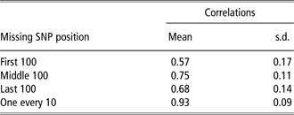
The effects of SNP location on prediction accuracy can be observed in Table 1 in which average correlations between actual and PLSR-predicted SNP genotypes for different scenarios are reported. Lowest correlations were obtained when markers to be predicted are located at the beginning or at the end of the chromosome. A slight increase in accuracy can be observed when SNP are located in the middle of the chromosome. The highest value was found for evenly spaced missing SNP. These results were expected, considering the decaying pattern of correlation between loci for increasing distances, and are in agreement with figures reported by Habier et al. (Reference Habier, Fernando and Dekkers2009) who had already used evenly spaced SNP to simulate LDM panels. In any case, the value of the mean correlation for the best scenario is notably high and may represent a useful indication for constructing an LDM platform without trait or breed constraints.
Mean correlations and related s.d. between 100 actual and predicted SNPs in each chromosome

SNP = single nucleotide polymorphism.
Step 2
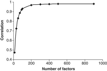
Figure 1 displays the pattern of mean correlations between 100 actual and PLSR-predicted SNP for increasing the number of extracted latent factors for the first chromosome. There is a rapid increase in prediction accuracy from 10 up to 100 factors (from 47% to 93%). A plateau of 98% is then reached when about 150 to 200 factors are extracted. These results indicate that the number of latent factors to be extracted should be higher or at least equal to the number of predicted SNP.
Pattern of the mean correlations between actual and predicted SNP for increasing the number of extracted factors during the PLSR procedure.

Step 3
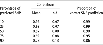
The variation in prediction accuracy for different numbers of SNP to be predicted is reported in Table 2. Moving from 10% to 75% missing SNP, there is a small decrease (∼6%) in the average correlation between actual and predicted genotypes. In any case, prediction accuracy is higher than 90% even when two-thirds of the SNP are predicted. It falls slightly below 0.80% when 90% of SNP have to be predicted. However, even in this case, the accuracy can be considered satisfactory. If confirmed on real data, the results of this study may indicate that a chip with 5.4 K SNP evenly spaced across the genome could represent a suitable base for reconstructing, with a reasonable accuracy, the profile of a high-density platform of 54 K SNP (i.e. the one currently used for cattle). In a recent study carried out with the bovine 54 K SNP, Weigel et al. (Reference Weigel, Van Tassell, O'Connell, VanRaden and Wiggans2010), using the algorithm implemented in fastPHASE 1.2 software (University of Washington TechTransfer Digital Ventures Program, Seattle, WA, USA), reported a proportion of correctly reconstructed missing SNP of about 0.88% when 90% SNP were predicted. Druet and Georges (Reference Druet and Georges2010) combined fastPHASE and Beagle (Browning and Browning, Reference Browning and Browning2007) algorithms to take into account both population (linkage disequilibrium) and familial (Mendelian segregation and linkage) information to predict missing genotypes. They found, with 50% missing genotypes, an imputation error of 3% and 1%, respectively, for sparse and dense marker maps. In this study, the proportion of correctly reconstructed SNP for 90% and 50% missing genotypes was 0.86 and 0.98, respectively (Table 2).
Mean correlations and related s.d. between actual and predicted SNPs for increasing percentage of predicted SNPs. Proportions of correct SNP prediction are also reported

SNP = single nucleotide polymorphism.
The SNP genotype profile of each animal was also well reconstructed by the PLSR method. When 90% SNP were predicted, >84% of animals presented a percentage of corrected SNP reconstruction ranging from 80% to 100%. Moreover, when predicted SNP were <75%, all animals had a proportion of corrected reconstructed SNP ranging from 95% to 100%.
Step 4
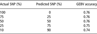
Accuracies displayed in Table 3 indicate that the use of PLSR-predicted SNP does not affect the estimation of GEBVs. Correlations between TBV and GEBV remain basically the same, moving from the scenario where all used SNP are actual to the one where 90% of marker genotypes are PLSR-predicted (Table 3). These results are similar to those obtained by Habier et al. (Reference Habier, Fernando and Dekkers2009) who reported a reduction in GEBV accuracy of about 4%, moving from an SNP panel density of 0.05 to 10 cM.
GEBV accuracies for different ratio of actual and predicted SNPs

GEBV = genomic breeding values; SNP = single nucleotide polymorphism.
Step 5
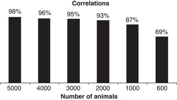
Finally, Figure 2 displays accuracies of SNP prediction obtained with different sizes of REF population. As the number of fully genotyped animals becomes smaller, correlations between actual and predicted SNP slowly decrease, reaching a value of 93% when the number of REF animals is twice (2000) the total number of SNP per chromosome. Correlations dramatically drop (<70%) for a number of fully genotyped animals equal to 600. Considering that on real data each bovine chromosome has on average 1000 to 1200 SNP after data editing, a minimum number of 2000 to 2500 fully genotyped animals could be enough to obtain reliable predictions from the PLSR method.
Mean correlations between actual and predicted SNP for different numbers of fully genotyped animals.

Conclusions
The use of LDM platforms in combination with a suitable computational algorithm able to predict the missing genotypes with respect to HDM chips is an option for reducing genotyping costs in GS programs. Savings could be used to enlarge the genotyped population, thus enhancing the efficiency of the breeding scheme. In thisstudy, the ability of the PLSR technique to predict missing SNP genotypes in LDM platforms was tested. The method correctly assigned from 86% to 98% of missing genotypes, when 90% and 50% SNP were predicted, respectively. Moreover, only a slight difference (2%) in GEBV accuracies was observed using actual SNP or a mixture of actual and predicted SNP. Finally, a size of around 2000 to 2500 fully genotyped animals with a 54 K SNP chip was found to be a reliable REF population to reconstruct the SNP profile of a PRED population of animals genotyped with an LDM chip containing 5 and 4 K evenly spaced SNP.
Acknowledgment
The research was funded by the Italian Ministry of Agriculture (Rome, Italy), grant SELMOL.