1. Introduction
Wall-sheared turbulent flows – pipes, channels and boundary layers – exhibit a spectrum of response modalities when drag-inducing elements are affixed to the bounding wall (Raupach, Antonia & Rajagopalan Reference Raupach, Antonia and Rajagopalan1991; Jimenez Reference Jimenez2004; Allen et al. Reference Allen, Shockling, Kunkel and Smits2007; Castro Reference Castro2007). For fully rough, inertia-dominated conditions – which encompass a broad range of important geophysical and engineering flows – drag-inducing elements augment wall-normal momentum fluxes. To establish governing parameters for these flows, we introduce  $h$ and
 $\delta$ as the aggregate element height and flow depth, respectively, friction velocity,
 $u_\tau$, and kinematic viscosity,
 $\nu$; these parameters can be used to compute the friction and roughness Reynolds numbers,
 $Re_\tau = u_\tau \delta / \nu$ and
 $Re_h = u_\tau h / \nu$, respectively. For ‘large’
 $Re_\tau$ values capable of attaining fully rough conditions, and in a Reynolds-averaged sense, rough-wall flows are composed of a roughness sublayer and inertial (outer) layer, where the thickness of the former,
 $x_{3,{RSL}}$, scales linearly with
 $h$ and is widely reported to exhibit values,
 $3 \lesssim x_{3,{RSL}}/h \lesssim 4$ (Grass Reference Grass1971; Raupach et al. Reference Raupach, Antonia and Rajagopalan1991; Ghisalberti Reference Ghisalberti2009). Note that, in this article, the first, second and third components of any vector,
 ${\boldsymbol {x}}$, denote its magnitude in the streamwise (
 $x_1$), spanwise (
 $x_2$) and wall-normal (
 $x_3$) directions, respectively; averaging of example quantity,
 $\phi (a)$, over example dimension,
 $a$, is denoted by
 $\langle \phi \rangle _a$. In the inertial sublayer above this, however, provided
 $\delta /h \gtrsim 40$ (where
 $\delta$ is the boundary layer thickness), Townsend's hypothesis states that a scale separation exists in which the outer-layer flow exhibits a universality independent of the roughness sublayer (with the exception of its response to
 $u_\tau$ and
 $\delta$; Townsend Reference Townsend1951; Jimenez Reference Jimenez2004). This has been largely confirmed by experiments (Wu & Christensen Reference Wu and Christensen2007, Reference Wu and Christensen2010), which demonstrate outer-layer similarity in the dynamical (hairpin vortex packets encapsulating low-momentum regions; Ganapathisubramani, Longmire & Marusic Reference Ganapathisubramani, Longmire and Marusic2003; Hutchins & Marusic Reference Hutchins and Marusic2007; Volino, Schultz & Flack Reference Volino, Schultz and Flack2007; Hong et al. Reference Hong, Katz, Meneveau and Schultz2012) and structural (two-point correlations; Wu & Christensen Reference Wu and Christensen2007, Reference Wu and Christensen2010) properties of smooth- and rough-wall turbulence.
Recent studies have shown that large-scale spatial heterogeneity in the distribution of elements – that is, variations at scales comparable to the flow depth,  $\delta$ – is itself a roughness parameter. Judicious variability in ostensibly ‘small’ elements – i.e. elements for which
 $\delta / h \gtrsim 40$ (Townsend Reference Townsend1951; Flack, Schultz & Connelly Reference Flack, Schultz and Connelly2007) – can induce a
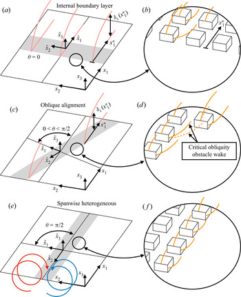
 $\delta$-scale flow response, thereby violating outer-layer similarity. We emphasize that quantifying deviation from outer-layer similarity is not the focus of this paper; for quantification of how large-scale heterogeneity drives deviation from outer-layer similarity, we direct interested readers to Awasthi & Anderson (Reference Awasthi and Anderson2018). For discussion, consider figure 1(a,c,e), which shows canonical heterogeneities composed of three adjacent regions, each with differing surface roughness height corresponding to ‘smooth’ and ‘rough’ (see annotation); for all cases, the dominant transport direction of the flow (streamwise) is aligned with
 $x_1$, while a local coordinate system,
 $\hat {\boldsymbol {x}}$, is introduced, which is normal to the heterogeneity and oblique to
 ${\boldsymbol {x}}$ at angle,
 $\theta$. Flow alignment orthogonal to the smooth-to-rough transition (panel a) results in production of turbulence across the transition and the formation of a new layer – the internal boundary layer (IBL) – which grows in thickness downstream (Antonia & Luxton Reference Antonia and Luxton1971; Wood Reference Wood1981; Garratt Reference Garratt1990; Bou-Zeid, Meneveau & Parlange Reference Bou-Zeid, Meneveau and Parlange2004) and begins at the transition, denoted by local coordinate,
 $x_1^{*}$. In contrast, when
 $\theta = {\rm \pi}/2$, the flow is parallel to the heterogeneity (see figure 1e) and the spanwise variability in imposed drag sustains Reynolds-averaged counter-rotating secondary cells (Mejia-Alvarez, Barros & Christensen Reference Mejia-Alvarez, Barros and Christensen2013; Willingham et al. Reference Willingham, Anderson, Christensen and Barros2013; Barros & Christensen Reference Barros and Christensen2014; Vanderwel & Ganapathisubramani Reference Vanderwel and Ganapathisubramani2015; Anderson et al. Reference Anderson, Barros, Christensen and Awasthi2015a; Kevin et al. Reference Kevin, Bai, Pathikonda, Nugroho, Barros, Christensen and Hutchins2017; Pathikonda & Christensen Reference Pathikonda and Christensen2017; Yang & Anderson Reference Yang and Anderson2017; Anderson et al. Reference Anderson, Yang, Shrestha and Awasthi2018; Chung, Monty & Hutchins Reference Chung, Monty and Hutchins2018; Medjnoun, Vanderwel & Ganapathisubramani Reference Medjnoun, Vanderwel and Ganapathisubramani2018; Kevin & Hutchins Reference Kevin and Hutchins2019; Anderson Reference Anderson2019). Annotations are provided for counter-rotating cells in figure 1(e), where prior work has shown flow response such that downwelling and upwelling are located above the relatively more and less rough regions of the surface, respectively (Willingham et al. Reference Willingham, Anderson, Christensen and Barros2013; Barros & Christensen Reference Barros and Christensen2014; Anderson et al. Reference Anderson, Barros, Christensen and Awasthi2015a); we stress that others have found the precise opposite flow response (Vanderwel & Ganapathisubramani Reference Vanderwel and Ganapathisubramani2015; Medjnoun et al. Reference Medjnoun, Vanderwel and Ganapathisubramani2018; Vanderwel et al. Reference Vanderwel, Stroh, Kriegseis, Frohnapfel and Ganapathisubramani2019). Yet more-recent studies have addressed the underlying conditions responsible for setting the secondary flow direction based on spacing attributes (Wangsawijaya et al. Reference Wangsawijaya, Baidya, Chung, Marusic and Hutchins2020), spacing and geometric attributes (Hwang & Lee Reference Hwang and Lee2018) and the implications for the aero-/hydrodynamic signature of spanwise-heterogeneous surfaces assembled with novel roughness attributes (Stroh et al. Reference Stroh, Schäfer, Frohnapfel and Forooghi2020). Panels (b, f) are ‘zoomed’ images of the elements responsible for imposing relatively ‘more rough’ conditions, where orange lines denote idealized wakes emanating from individual elements (Raupach Reference Raupach1992; Yang et al. Reference Yang, Sadique, Mittal and Meneveau2016); these wakes eventually homogenize due to ambient shear within the inertial layer (Anderson, Li & Bou-Zeid Reference Anderson, Li and Bou-Zeid2015b; Zhu et al. Reference Zhu, Iungo, Leonardi and Anderson2016).
Schematic illustrating idealized flow response to streamwise heterogeneity (a,b), oblique alignment (c,d) and spanwise heterogeneity (e, f), where streamwise (a,b) and spanwise (e, f) heterogeneity will yield an IBL (Antonia & Luxton Reference Antonia and Luxton1971; Wood Reference Wood1981; Andreopoulos & Wood Reference Andreopoulos and Wood1982; Garratt Reference Garratt1990; Bou-Zeid et al. Reference Bou-Zeid, Meneveau and Parlange2004; Bou-Zeid, Meneveau & Parlange Reference Bou-Zeid, Meneveau and Parlange2005) and streamwise secondary cells (Willingham et al. Reference Willingham, Anderson, Christensen and Barros2013; Anderson et al. Reference Anderson, Barros, Christensen and Awasthi2015a; Yang & Anderson Reference Yang and Anderson2017; Medjnoun et al. Reference Medjnoun, Vanderwel and Ganapathisubramani2018; Anderson Reference Anderson2019), respectively, as per the figure annotations. Here,  $x_1^{*}$ denotes the IBL origin. (b,d, f) Are expansion images, as per the annotation, of the roughness sublayer flow process across the heterogeneity leading edge, where (d) highlights the emergence of successive shelterings (Raupach Reference Raupach1992; Yang et al. Reference Yang, Sadique, Mittal and Meneveau2016) attained at the critical obliquity.

The majority of prior research in the area of large-scale roughness heterogeneity – including scenarios resembling those shown in figure 1 – address arrangements leading to an IBL (figure 1a) or to streamwise counter-rotating secondary cells (figure 1e). However, scenarios with flow alignment precisely orthogonal or parallel to the heterogeneity are likely to be the exception – not the norm – in flow systems of practical importance; alignments with some degree of obliquity are expected to be far more common (Anderson Reference Anderson2020). Consider, for example, atmospheric boundary layer flows encountering large-scale landscape heterogeneity at oblique angles (Bou-Zeid et al. Reference Bou-Zeid, Anderson, Katul and Mahrt2020; Stoll et al. Reference Stoll, Gibbs, Salesky and Anderson2020), or hydrodynamic flows encountering panel texture variability at oblique angles. Figure 1(c) illustrates such an example of flow-heterogeneity obliquity, with  $0 < \theta < {\rm \pi}/2$.
1.1. Regime collapse
In prior work, Anderson (Reference Anderson2020) used large-eddy simulation (LES) of fully rough turbulent channel flow to explore flow response to flow-roughness obliquity. Anderson (Reference Anderson2020) showed that, as the obliquity angle,  $\theta$, is increased from zero (i.e. figure 1a–c), an IBL-like response persists, which is annotated in figure 1(c). Anderson (Reference Anderson2020) found also that the oblique alignments yield a Reynolds-averaged spanwise velocity component, a product of the oblique drag distribution. Results showed that the persistent IBL-like response and spanwise velocity remain up to
 $\theta = 3 {\rm \pi}/ 8$, before abruptly collapsing – in its place, Reynolds-averaged secondary cells form under the mechanisms already established in preceding work (Anderson et al. Reference Anderson, Barros, Christensen and Awasthi2015a). If
 $\theta = 0$ and
 $\theta = {\rm \pi}/ 2$ induce an IBL and counter-rotating secondary cells, respectively, regime transition is a necessary consequence of oblique alignments – however, the abrupt and non-monotonic nature of the transition compels additional work.
1.2. This study
For this article, we have performed a large-scale assessment of salient parameters affecting flow response to flow-roughness obliquity: obliquity angle,  $\theta$, element height,
 $h$, and spacing between adjacent rows of elements,
 $s$ (i.e. spacing in the
 $\hat {x}_1$ direction). In order to specifically target the aforementioned regime collapse, which occurred for
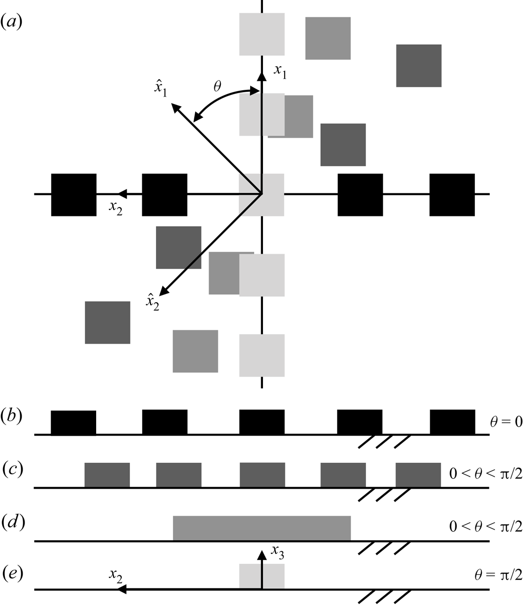
 $3 {\rm \pi}/ 8 \leqslant \theta \leqslant {\rm \pi}/ 2$, we have used a series of additional intermediate obliquities to isolate the critical obliquity (discussion to follow). Results presented herein will show that the persistent IBL-like response, and the sudden regime collapse at critical obliquity, are a product of successive element shelterings (Raupach Reference Raupach1992; Yang et al. Reference Yang, Sadique, Mittal and Meneveau2016). This effect can be appreciated from figure 2(a), which shows an idealized distribution of cuboid roughness elements at a series of obliquities ranging from
 $\theta = 0$ (black) to
 $\theta = {\rm \pi}/ 2$ (lightest grey). Figure 2(b–e) shows the corresponding spanwise–wall-normal element projection from an ‘upflow’ observer, where for
 $\theta = {\rm \pi}/2$ only a single block is visible to the observer.
Schematic illustration of representative wall-mounted cube arrangements used to impose large-scale surface roughness heterogeneity. (a) Shows Cartesian coordinate systems,  ${\boldsymbol {x}}$ and
 $\hat {\boldsymbol {x}}$, where the former is used for LES while the latter is aligned such that
 $\hat {x}_1$ is normal to the heterogeneity;
 $\hat {\boldsymbol {x}}$ is oblique to
 ${\boldsymbol {x}}$ in the streamwise–spanwise plane by angle,
 $\theta$. (a) Shows cube arrangements for
 $\theta = 0$ (black),
 $0 < \theta < {\rm \pi}/2$ (dark grey, grey), and
 $\theta = {\rm \pi}/2$ (light grey). For the idealized cases shown in (a), (b–e) show the corresponding exposed frontal area based on visualization in the spanwise–wall-normal plane viewed from an ‘upflow’ location.

The aero-/hydrodynamic implications of the ‘observer’ view is formally recognized and quantified via the frontal-area index,
 \begin{equation} \lambda_f(\theta) = \left.\displaystyle\int_{\mathrm{d}^{2} \,{\boldsymbol{x}}} \mathcal{R} \left( \partial_1 h({\boldsymbol{x}};\theta) \right) \mathrm{d}^{2}\, {\boldsymbol{x}} \right/ \displaystyle\int_{\mathrm{d}^{2}\, {\boldsymbol{x}}} \,\mathrm{d}^{2}\, {\boldsymbol{x}}, \end{equation}
where  $\mathcal {R}(x)$ is the ramp function:
 $\mathcal {R}(x) = 0$ and
 $x$ for
 $x < 0$ and
 $x \geqslant 0$, respectively, while
 $\partial _1 h$ is the streamwise gradient of height (not to be confused with
 $d_1$ in figure 3(e) and accompanying text). Used in this manner, the ramp function isolates the frontal area of obstacles ‘seen’ by the flow and upon which fluxes of momentum are delivered. The parameter
 $\mathrm {d}^{2} {\boldsymbol {x}}$ represents the
 $x_1- x_2$ plane, and
 $\partial _1 h ({\boldsymbol {x}};\theta )$ is the streamwise partial derivative of height with respect to
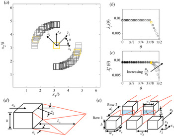
 $x_1$ for the range of rough surfaces considered. Figure 3(a) shows an idealized distribution of three cuboid elements in the
 $x_1-x_2$ plane, where
 $h/\delta = 0.25$ for the elements; from black to grey corresponds to
 $\theta = 0$ and
 ${\rm \pi} /2$, respectively, where
 $\hat {\boldsymbol {x}}$ is superimposed for reference. Figure 3(b) shows the corresponding frontal-area index with equivalent black-to-grey colour coding. As informed by figure 2,
 $\lambda _f (\theta )$ is constant for a range of obliquities, before abruptly declining as the frontal profiles of the cuboids begin to overlap one another; the first value of
 $\theta$ at which
 $\lambda _f (\theta )$ begins declining is noted with yellow in figure 3(a,b). This arrangement is strikingly similar to the critical obliquity at which the aforementioned regime collapse occurred in Anderson (Reference Anderson2020).
Cuboid elements and flow response. (a) Shows streamwise–spanwise visualization of a series of surfaces composed of three wall-mounted cubes, where the surfaces differ based on a variable obliquity angle from  $\theta = 0$ (black) to
 $\theta = {\rm \pi}/2$ (lightest grey). (b,c) Show frontal-area index,
 $\lambda _f (\theta )$ (1.1) and compensated frontal-area index,
 $\lambda _f^{*} (\theta )$ (1.2), respectively, where the largest value of
 $\theta$ for which
 $\lambda _f$ and
 $\lambda _f^{*}$ begin decreasing is hereafter named the critical obliquity,
 $\theta _c$, and is marked in yellow in (b,c). In (c), profiles are shown for ‘input’ values,
 $u_h/u_\tau = 10$ (squares), 5 (circles) and 2.5 (stars); see also (1.3). The block arrangement for this ‘turning point’ obliquity angle is also shown in yellow in (a) for perspective. (d) Shows an idealized cuboid with wake and sheltering attributes superimposed: element height velocity,
 $u_h$, sheltering length,
 $L_s$, and sheltering angle,
 $\theta _s$, where red lines represent the limits of the element-affected spatial volume. (e) Shows additional wake and sheltering attributes due to two successive rows of elements:
 $w_e$ and
 $b_e$ are the element width and length, respectively,
 $d_1$ and
 $d_2$ are the streamwise and spanwise spacing between elements, respectively,
 $h_s$ and
 $w_s$ are the sheltered height and width, respectively, and
 $A_s = h_s d_s$ is the sheltered area.

In addition to the ‘observer’ view deductions of aero-/hydrodynamic effects, as per (1.1), some rudimentary estimates of frontal-area index can be attained via consideration of the wake recovery associated with each element. Implicit to the use of (1.1) is the assumption that successive downflow elements are entirely sheltered by the presence of any upflow element; this approach objectively fails to incorporate the sheltering effect of elements, which allows for eventual flow recovery and associated aero-/hydrodynamic loading (Raupach Reference Raupach1992; Yang et al. Reference Yang, Sadique, Mittal and Meneveau2016). Figure 3(d) shows an idealized cuboid image with annotations for key parameters associated with the sheltering effect: element height velocity,  $u_h$, sheltering length,
 $L_s$, and sheltering angle,
 $\theta _s$, where red lines represent the limits of the element-affected spatial volume. Figure 3(e) shows yet more information – this time associated with the influence of one row of elements upon another – where
 $w_e$ and
 $b_e$ are the element width and length, respectively,
 $d_1$ and
 $d_2$ are the streamwise and spanwise spacings between elements, respectively,
 $h_s$ and
 $w_s$ are the sheltered height and width, respectively, and
 $A_s = h_s d_s$ is the sheltered area; again, red lines are used to represent the limits of the element-affected spatial volumes, which highlights how the sheltering effect enables successive elements to absorb momentum. The sheltering effect, and the implications of sheltering for the frontal area index, can readily be captured through a compensated frontal-area index,
 \begin{equation} \lambda_f^{*}(\theta) = \left.\displaystyle\int_{\mathrm{d}^{2} \,{\boldsymbol{x}}} \mathcal{R} \left( \partial_1 h^{*}({\boldsymbol{x}};\theta) \right) \mathrm{d}^{2}\, {\boldsymbol{x}} \right/\displaystyle\int_{\mathrm{d}^{2}\, {\boldsymbol{x}}} \mathrm{d}^{2}\, {\boldsymbol{x}}, \end{equation}
where  $h^{*}$ is the height distribution, compensated for successive wake shelterings (i.e. the white frontal areas in figure 3e). The wake sheltering angle,
 $\theta _s$, can be calculated with the wake expansion rate, via a model established by Yang et al. (Reference Yang, Sadique, Mittal and Meneveau2016)
 \begin{equation} \tan \theta_s = C_{\theta_s} \dfrac{u_\tau}{u_h}, \end{equation}
where  $u_\tau$ is an a priori-defined friction velocity,
 $u_h$ is mean velocity at roughness element height – to be recovered a posteriori from LES – and
 $C_{\theta _s}$ is a geometry-dominated coefficient of order unity that can also be calculated via
 \begin{equation} C_{\theta_s} = \left( \dfrac{6}{C_{D}} \dfrac{u_\tau}{u_h} \right) \left( \dfrac{1}{3}+\dfrac{2h}{3w_e} \right), \end{equation}
where  $C_{D}$ is a drag coefficient associated with the roughness elements, and is here estimated as
 $C_{D}\approx 1.4$ (Akins, Peterka & Cermak Reference Akins, Peterka and Cermak1977; Hussain & Lee Reference Hussain and Lee1980; Curley & Uddin Reference Curley and Uddin2015). In the absence of a pre-defined
 $C_{D}$, it would also be acceptable to impose
 $C_{D} \rightarrow 1$ as per the inertia-dominated (fully rough) flow conditions. For the cuboid elements considered in figure 3(a),
 $w_e/\delta = b_e/\delta \approx 0.5$, and
 $h/\delta$ = 0.25, rendering the sheltering length,
 $L_s = h/\tan \theta _s$, the sheltering height
 $h_s = (L_s - d_1) \tan \theta _s$ (see also figure 3e). This relation shows that
 $h^{*} = h - h_s$ and
 $w_s = w_e$ for the case of streamwise-aligned blocks, while (1.3) and (1.4) provide the framework for
 $\lambda _f^{*}$ computation of the more complex oblique arrangements to be considered herein. For the cases considered in figure 3(a),
 $d_1$ and
 $d_2$ vary with the block position, while
 $w_e/\delta = b_e/\delta = 0.5$.
For assumed values,  $u_h/u_\tau = 10$ (squares), 5 (circles) and 2.5 (stars), and for the idealized block arrangements shown in figure 3(a), (1.3) and (1.4) are used to compute
 $\lambda _f^{*}(\theta )$, which is shown in figure 3(c). These values of
 $u_h/u_\tau$ are consistent with values reported in complementary studies (Anderson et al. Reference Anderson, Li and Bou-Zeid2015b; Zhu et al. Reference Zhu, Iungo, Leonardi and Anderson2016; Zhu & Anderson Reference Zhu and Anderson2018) and, more importantly, the results indicate a consistent critical obliquity. As expected, the values are equivalent to
 $\lambda _f(\theta )$ (figure 3b) for
 $\theta \lesssim 3{\rm \pi} / 8$, since there is no capacity for sheltering. However, as sheltering begins to affect the aero-/hydrodynamic signature of the surface (figure 3d,e), for
 $\theta \gtrsim 3 {\rm \pi}/ 8$,
 $\lambda _f$ decreases relatively faster since there is no generality to incorporate the partially available frontal area of downflow blocks. In both cases, we find
 $\theta _c = 22 {\rm \pi}/ 56$.
In the interest of thorough treatment, we note also that the plan-area index is commonly cited alongside the frontal-area index as a roughness indicator (Zhu et al. Reference Zhu, Iungo, Leonardi and Anderson2016; Zhu & Anderson Reference Zhu and Anderson2018)
 \begin{equation} \lambda_p(\theta) = \left.\displaystyle\int_{\mathrm{d}^{2}\, {\boldsymbol{x}}} \mathcal{H} \left( h({\boldsymbol{x}};\theta) \right) \mathrm{d}^{2}\, {\boldsymbol{x}} \right/ \displaystyle\int_{\mathrm{d}^{2}\, {\boldsymbol{x}}} \mathrm{d}^{2}\, {\boldsymbol{x}}, \end{equation}
where  $\mathcal {H}$ is the Heaviside step function. It will be shown that
 $\lambda _p \neq \lambda _p (\theta )$, although
 $\lambda _p$ is used widely in prognostic modelling of bulk aero-/hydrodynamic parameters (Macdonald, Griffiths & Hall Reference Macdonald, Griffiths and Hall1998; Zhu et al. Reference Zhu, Iungo, Leonardi and Anderson2016).
As shown in these developments, successive element shelterings have major implications for the interpretation of the aforementioned regime collapse from a persistent IBL-like response to the presence of counter-rotating streamwise secondary cells. In Anderson (Reference Anderson2020), this was not considered, nor was the influence of element height or  $\hat {x}_1$-aligned spacing between adjacent ‘rows’ of elements.
In this article, LES has been used to perform a comprehensive parameter sweep to capture the influence of obliquity, element height and  $\hat {x}_1$-aligned spacing. The results will be consolidated in a manner than isolates parameter influence; the results are used to definitively attribute the aforementioned abrupt regime collapse to successive element shelterings. As noted, we have used cuboid elements, which can be readily implemented as bluff obstacles in our LES code (discussion to follow). Other roughness elements have been used – for example, complex roughness by Christensen and company (Mejia-Alvarez et al. Reference Mejia-Alvarez, Barros and Christensen2013; Barros & Christensen Reference Barros and Christensen2014; Pathikonda & Christensen Reference Pathikonda and Christensen2017), LEGO® elements by Ganapathisubramani and company (Vanderwel & Ganapathisubramani Reference Vanderwel and Ganapathisubramani2015; Medjnoun et al. Reference Medjnoun, Vanderwel and Ganapathisubramani2018; Vanderwel et al. Reference Vanderwel, Stroh, Kriegseis, Frohnapfel and Ganapathisubramani2019) and herringbone-type distributions by Hutchins and company (Nugroho, Hutchins & Monty Reference Nugroho, Hutchins and Monty2013; Kevin et al. Reference Kevin, Bai, Pathikonda, Nugroho, Barros, Christensen and Hutchins2017; Chung et al. Reference Chung, Monty and Hutchins2018; Kevin & Hutchins Reference Kevin and Hutchins2019). It is beyond the scope of this article to consider the influence of element geometry. However, given the preceding discussion on successive element shelterings and regime collapse, we envision this as an important area for future work. In § 2, details of the LES code and cases considered are outlined (§§ 2.1 and 2.2, respectively). Discussion of results is presented in § 3. Concluding remarks are presented in § 4.
2. Numerical approach and cases
2.1. LES code
The spatially filtered incompressible momentum transport equation is solved,  ${D}_t \tilde {\boldsymbol {u}}({\boldsymbol {x}},t) = {\boldsymbol {f}}({\boldsymbol {x}},t)$, where the grid-filtering operation is performed via convolution with the filtering kernel,
 $\tilde {\boldsymbol {u}}({\boldsymbol {x}},t) = G_{\varDelta } \star {\boldsymbol {u}}({\boldsymbol {x}},t)$, where
 $\widetilde {\ldots }$ denotes a grid-filtered quantity.
 ${\boldsymbol {f}} = - \rho ^{-1} \boldsymbol {\nabla } p - \boldsymbol {\nabla } \boldsymbol {\cdot } {\boldsymbol {\tau }} + {\boldsymbol {e}}_1 {\varPi } + {\boldsymbol {f}}_b$, where
 $\rho$ is density,
 $\boldsymbol {\nabla } p$ is a pressure correction required to preserve a divergence-free (incompressible) flow,
 $\boldsymbol {\nabla } \boldsymbol {\cdot } \tilde {\boldsymbol {u}} = 0$,
 ${\boldsymbol {\tau }} = \widetilde {{\boldsymbol {u}}^{\prime } \otimes {\boldsymbol {u}}^{\prime }}$ is the subgrid-scale stress tensor, where
 ${\boldsymbol {u}}^{\prime } = {\boldsymbol {u}} - \tilde {\boldsymbol {u}}$,
 ${\varPi } = \rho ^{-1} \,\mathrm {d} P_0 / \mathrm {d} x_1$ is an imposed pressure gradient and
 ${\boldsymbol {f}}_b$ is a body force. Note that the shear-normalized viscous stress tensor,
 $Re_\tau ^{-1} \nabla ^{2} \tilde {\boldsymbol {u}}$, is omitted since
 $Re_\tau = u_\tau \delta \nu ^{-1} \sim {O}(10^{7})$ for the inertia-dominated (fully rough) flow conditions typical of geophysical/engineering wall-sheared turbulence, where
 $u_\tau$ is the shear velocity,
 $\delta$ is flow depth (channel half-height) and
 $\nu$ is kinematic viscosity. A solenoidal velocity field is maintained by computing the divergence of the momentum transport equation,
 ${D}_t [ \boldsymbol {\nabla } \boldsymbol {\cdot } \tilde {\boldsymbol {u}}({\boldsymbol {x}},t) ] = \boldsymbol {\nabla } \boldsymbol {\cdot } {\boldsymbol {f}}({\boldsymbol {x}},t)$, applying the divergence-free condition,
 $\boldsymbol {\nabla } \boldsymbol {\cdot } \tilde {\boldsymbol {u}} = 0$ and solving the resultant pressure Poisson equation with Neumann conditions at the domain top and bottom,
 $\partial \tilde {p}/\partial x_{3} |_{x_3 / \delta = 1} = 0$ and
 $\partial \tilde {p}/\partial x_{3} |_{x_3 / \delta = 0} = 0$, respectively. Spectral discretization is used in the horizontal directions, while vertical gradients are evaluated with centred second-order finite differencing. Owing to horizontal spectral discretization, periodic boundary conditions are imposed on the vertical ‘walls’ of the domain.
The deviatoric component of the subgrid-scale stresses,  ${\boldsymbol {\tau }}^{d}$, is evaluated using the eddy viscosity modelling approach,
 ${\boldsymbol {\tau }}^{d} = {\boldsymbol {\tau }} - \frac {1}{3} {\boldsymbol {\delta }} : {\boldsymbol {\tau }} = - 2 \nu _t \tilde {{\boldsymbol{\mathsf{S}}}}$, where
 $\nu _{t} = (C_s \varDelta )^{2} |\tilde {{\boldsymbol{\mathsf{S}}}}|$ is the turbulent viscosity,
 $C_s$ is the Smagorinsky coefficient,
 $\varDelta$ is the filter size,
 $\tilde {{\boldsymbol{\mathsf{S}}}} = \frac {1}{2}(\partial \tilde {\boldsymbol {u}} + \partial \tilde {\boldsymbol {u}}^{T})$ is the resolved strain-rate tensor and
 $|\tilde {{\boldsymbol{\mathsf{S}}}}| = (2 \tilde {{\boldsymbol{\mathsf{S}}}} {\boldsymbol {:}}\tilde {{\boldsymbol{\mathsf{S}}}} )^{1/2}$ is the magnitude of the resolved strain-rate tensor. In the present study,
 $C_s$ is evaluated dynamically during LES with the Lagrangian scale-dependent dynamic subgrid-scale (SGS) model of Bou-Zeid et al. (Reference Bou-Zeid, Meneveau and Parlange2005). The present LES code has been used in many studies of inertia-dominated, rough-wall turbulence (see Anderson et al. (Reference Anderson, Barros, Christensen and Awasthi2015a) and references therein).
The computational mesh is discretized via  $\varDelta _{1} = L_{1}/N_{1}$,
 $\varDelta _{2} = L_{2}/N_{2}$ and
 $\varDelta _{3} = L_{3}/N_{3}$, where
 $\{ L_{1}, L_{2}, L_{3}\}$ is the domain spatial extent and
 $\{N_{1}, N_{2}, N_{3} \}$ is grid resolution. The lower wall momentum fluxes are modelled with a hybrid approach. For locations where
 $h(x_1,x_2) > \varDelta _{3} / 2$ (i.e. an element is protruding into the vertically staggered computational mesh), the drag force imposed on the flow by
 $h ( x_1 , x_2 )$ is captured with the body force,
 ${\boldsymbol {f}}_b$, appearing in the grid-filtered momentum transport equation (Anderson & Meneveau Reference Anderson and Meneveau2010; Anderson Reference Anderson2012); these regions are conceptually equivalent to ‘more rough’ regions, which would exhibit a relatively larger roughness length (i.e.
 $z_{0,h}$). For locations where
 $h(x_1,x_2) < \varDelta _{3}/2$ – i.e. flat regions surrounding the large elements – surface stress is modelled under logarithmic (equilibrium) conditions with baseline roughness length,
 $z_0/\delta = 5 \times 10^{-6}$ (Anderson & Meneveau Reference Anderson and Meneveau2010). This work is, thus, entirely predicated upon local (space–time) efficacy of the logarithmic law (i.e. the presumption of local space–time equilibrium conditions in a complex flow). In the strictest possible sense, local equilibrium never exists, but in recent years there has been widespread use of the logarithmic law in such conditions. Bou-Zeid et al. (Reference Bou-Zeid, Meneveau and Parlange2005) demonstrated that such a use of the logarithmic law could be successful in channel flows, and many immersed boundary methods leverage the logarithmic law for prescription of peripheral stresses (Graham & Meneveau Reference Graham and Meneveau2012 and references therein). Given the absence of an existing experimental dataset for equivalent cases, the influence of the logarithmic law upon the resultant flow cannot be quantified, nor would such an effort fall within the scope of this work. It is stressed, however, that results from this wall-modelling protocol have been compared against a variety of datasets in the literature of complementary studies, and in all cases reasonable agreement has been attained (Willingham et al. Reference Willingham, Anderson, Christensen and Barros2013; Anderson et al. Reference Anderson, Barros, Christensen and Awasthi2015a; Zhu et al. Reference Zhu, Iungo, Leonardi and Anderson2016).
2.2. Cases
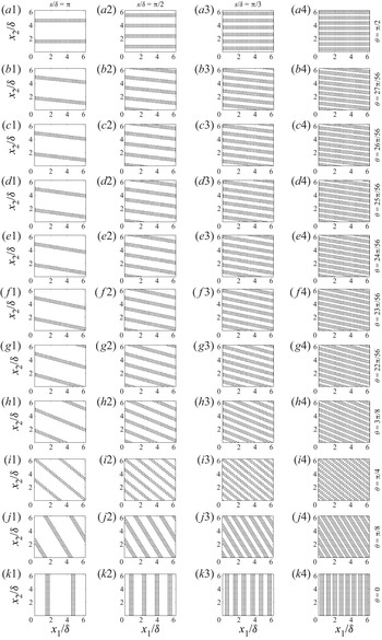
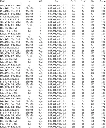
The aforementioned LES code has been used to model flow over the cases shown in figure 4, where the  $\hat {x}_1$ spacing between adjacent rows decreases from left to right, while obliquity angle increases from bottom to top. Anderson (Reference Anderson2020) considered cases shown in figure 4(a1,h1,i1,j1,k1), and reported the aforementioned critical obliquity and regime collapse that compels additional cases in the range,
 $3 {\rm \pi}/ 8 < \theta < {\rm \pi}/2$, which correspond to all cases encompassed by (b1–b4) to (g1–g4). It is for this reason that we include these additional cases herein, which pose special challenges for incorporation within the LES code due to the requirement of periodic boundary conditions. Figure 3 and accompanying text ((1.1) and (1.2) showed that
 $\theta _c = 22 {\rm \pi}/ 56$, which corresponds to ‘F’ cases in table 1. As per table 1, case names are based on a combination of three possible symbols:
 \begin{equation} \mathrm{Case} \equiv \underbrace{\left(\mathrm{Symbol}\ 1\right)}_{\substack{\mathrm{Obliquity},\ \theta \\ \mathrm{A\ to\ K}}} \ \underbrace{\left( \mathrm{Symbol}\ 2\right)}_{\substack{\mathrm{Spacing},\ s \\ \mathrm{1\ to\ 4}}} \ \underbrace{\left( \mathrm{Symbol}\ 3\right)}_{\substack{\mathrm{Height},\ h \\ \mathrm{a\ to\ d}}}. \end{equation}
For the cases with  $\theta = 0$,
 ${\rm \pi} /8$,
 ${\rm \pi} /4$,
 $3{\rm \pi} /8$ and
 ${\rm \pi} /2$, periodicity is assured for specific values of
 $\hat {x}_1$-normal spacing. For cases with
 $3 {\rm \pi}/ 8 < \theta < {\rm \pi}/2$, periodicity can only be attained with the use of domains with longer streamwise extent; for plotting purposes, (b1–b4) to (g1–g4) have been truncated at
 $x_1/\delta = 2 {\rm \pi}$. Table 1 provides quantitative details of salient case attributes, where values of
 $L_1/\delta$ are shown; note that the computational mesh discretization is constant for the cases considered, where
 $N_1$ is proportionately increased with
 $L_1/\delta$. Results of resolution sensitivity testing are not shown here, as this has been performed for a variety of prior studies based upon the same code (Yang et al. Reference Yang, Sadique, Mittal and Meneveau2016; Anderson Reference Anderson2019).
Streamwise–spanwise visualization of surfaces considered in present study, where left-to-right and bottom-to-top correspond to directions of decreasing spacing and increasing obliquity, respectively; annotations provided at right for obliquity, while left, second from left, second from right, and right columns correspond to  $s/\delta = {\rm \pi}$,
 ${\rm \pi} /2$,
 ${\rm \pi} /3$ and
 ${\rm \pi} /4$, respectively. Note that for cases with
 $22 {\rm \pi}/ 56 \leqslant \theta \leqslant 27 {\rm \pi}/ 56$ (i.e. b1–g4), the domains have been truncated in
 $x_1$ for the purpose of surface visualization; as per table 1, the domain streamwise extent for these cases is necessarily larger in order to impose periodic (in
 $x_1$ and
 $x_2$) surfaces. Additional surface details are reported in table 1. Surfaces shown in (a1–a4) and (k1–k4) will yield canonical streamwise counter-rotating secondary cells and an IBL, respectively; all intermediate cases correspond to oblique alignments (Anderson Reference Anderson2020).

Summary of key simulation attributes and reporting of varied parameters: obliquity,  $\theta$, spacing,
 $s/\delta$, and element height,
 $h/\delta$. Note that
 $L_1/\delta \neq L_2/\delta$ for ‘B’ to ‘G’ cases; for these cases, periodicity in
 $x_1$ and
 $x_2$ requires the use of domains with relatively greater streamwise extent. For computational mesh consistency, streamwise discretization is proportionately increased for these cases.

In addition to obliquity, we have also systematically recorded the influence of the  $\hat {x}_1$-aligned spacing between adjacent rows of elements, which is denoted by
 $s / \delta$ in table 1. For the case of spanwise heterogeneity (a1–a4), the spacing values considered –
 $s/\delta \approx 0.78$, 1.05, 1.57 and 3.14 – encompass a range of critically important values in the so-called ‘roughness’, ‘intermediate’ and ‘topography’ regimes, as per Yang & Anderson (Reference Yang and Anderson2017). Medjnoun et al. (Reference Medjnoun, Vanderwel and Ganapathisubramani2018) later speculated on this with their ‘Significance’ metric. In both Yang & Anderson (Reference Yang and Anderson2017) and Medjnoun et al. (Reference Medjnoun, Vanderwel and Ganapathisubramani2018), the intensity of turbulent secondary flows is strongest for
 $s/\delta \approx 1$. Finally, and for completeness, we have considered four values of element height, denoted by
 $h/\delta$ in table 1. The values, of course, correspond to
 $5 \leqslant \delta /h \leqslant 20$, thereby precluding formation of a roughness-invariant outer-layer structure (Townsend Reference Townsend1951; Flack et al. Reference Flack, Schultz and Connelly2007); the complex arrangements considered herein further inhibit outer-layer similarity via the sustenance of
 $\delta$-scale wakes emanating from the surface heterogeneities.
In order to comprehensively assess the role of these three parameters – obliquity, height and  $\hat {x}_1$-aligned spacing – a total of 176 cases have been considered; figure 4 shows
 $x_1 - x_2$ visualization of 44 subset cases showing the variation of spacing (horizontal) and obliquity (vertical). We consider cuboid elements, which follows prior work (Yang & Anderson Reference Yang and Anderson2017; Anderson Reference Anderson2019, Reference Anderson2020). Although the element heights vary, the width and depth were constant at
 $w_e/\delta = b_e/\delta = {\rm \pi}/32$; readers will quickly note that
 $w_e/\varDelta _{1} = ({\rm \pi} /32)/(L_{1}/N_{1}) = 2$, or 4 computational mesh points per level. The element spacing,
 $d_1/\delta = d_2/\delta = {\rm \pi}/32$ (see also figure 3d), and was constant between the cases. These ratios can alternatively be defined with respect to element height, where
 $d_1/h = d_2/h \approx 2$ for cases with
 $h/\delta = 0.05$ and
 $d_1/h = d_2/h \approx 0.5$ for cases with
 $h/\delta = 0.2$. These values render all cases as definitively ‘d’-type roughness (Raupach Reference Raupach1992; Jimenez Reference Jimenez2004), where inadequate spacing precludes complete flow reattachment in the roughness sublayer. It is certainly possible that, for more sparse element arrangements, with
 $d_1/h = d_2/h \sim \mathcal {10^{0}}$, the bulk aerodynamic signature would differ by minimizing element sheltering. Given the already extensive scope of this work, such an investigation cannot be made. Prior complementary work with the code described in § 2.1 has shown no discernible sensitivity to computational mesh resolution (Wang & Anderson Reference Wang and Anderson2018; Zhu & Anderson Reference Zhu and Anderson2018).
Within the main narrative, results will be shown for all cases summarized in table 1, with computational mesh resolution,  $\{N_{1}, N_{2}, N_{3} \} = \{128, 128, 128 \}$, and spatial extent,
 $\{L_{1}/\delta , L_{2}/\delta , L_{3}/\delta \} = \{2 {\rm \pi}, 2 {\rm \pi}, 1\}$, unless otherwise noted. In all cases, the grid-filtered momentum transport equations are numerically integrated until the flow attains temporal statistical homogeneity; the transport equations are then further advanced to recover Reynolds-averaged turbulence statistics. Turbulence statistics shown herein are based upon a shear-normalized averaging (large-eddy turnover) time,
 $\delta _t N_t U_0 \delta ^{-1} \gtrsim 10^{3}$, where
 $\delta _t$ is the dimensional time step,
 $N_t$ is the number of compute time steps associated with time averaging and
 $U_0$ is the dimensional centreline velocity, i.e.
 $U_0 = u_\tau \langle \tilde {u}_1 \rangle _{12t} (x_3/\delta = 1)$. In numerous prior studies, this averaging time has been consistently used to recover Reynolds-averaged quantities and, thus, to quantify turbulence statistics (Anderson & Meneveau Reference Anderson and Meneveau2010; Graham & Meneveau Reference Graham and Meneveau2012; Anderson et al. Reference Anderson, Barros, Christensen and Awasthi2015a).
3. Results
In the interest of brevity, only a subset of possible results are presented, all of which are chosen to demonstrate the influence of element height,  $\hat {x}_1$-aligned spacing and obliquity on flow response. We have already provided developmental information on the role of element frontal-area index, and implications for the aforementioned regime collapse (§§ 1.1 and 1.2; Anderson Reference Anderson2020). In addition, we once more emphasize that regime transition is imposed by the prescribed obliquity range: since
 $\theta = 0$ and
 $\theta = {\rm \pi}/ 2$ induce an IBL and counter-rotating secondary cells, respectively, regime transition is a necessary consequence of oblique alignments. In the following section, flow response modalities will be presented and summarized, all of which are consistent with the notion that successive element shelterings – beginning at
 $\theta \gtrsim 3 {\rm \pi}/ 8$ – preclude the formation of new IBLs, and provide the basis for emergence of quasi-streamwise-aligned counter-rotating secondary cells. We report, too, that this response proceeds monotonically across the range of element height and spacing values considered.
We have used time-, plane- and volume-averaged velocity to study the influence of variable element height, obliquity and spacing between adjacent rows of elements. We have, thus, defined the critical obliquity based only on the statistics of the large-scale velocity, but other quantities could have also been used to define the critical obliquity in terms of large-scale rotation, etc. In the interest of maintaining topical focus, such quantities have not been used. Finally, in Anderson (Reference Anderson2020), a prognostic roughness model was presented for oblique flow-roughness alignments; efficacy of this model is tested for the much-larger parameter range considered herein (see also table 1).
3.1. Parametric study results
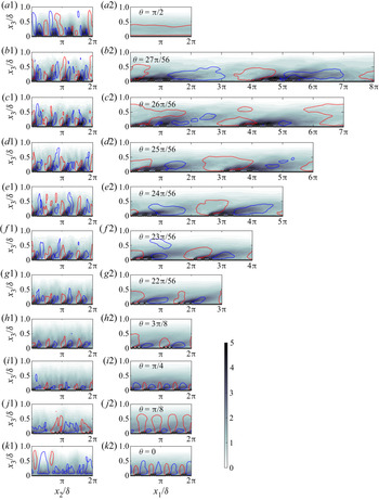
Figure 5 shows colour flood contours for turbulent kinetic energy,  $\langle k \rangle _t ({\boldsymbol {x}}) = \langle (\tilde {\boldsymbol {u}}^{\prime } {\boldsymbol {:}} \tilde {\boldsymbol {u}}^{\prime })/2 + \mathrm {Tr}({\boldsymbol {\tau }}) \rangle _t ({\boldsymbol {x}})$, with isocontours of vertical velocity superimposed corresponding to
 $\langle \tilde {w} \rangle _t ({\boldsymbol {x}}) = 1.0$ (red) and
 $\langle \tilde {w} \rangle _t ({\boldsymbol {x}}) = -1.0$ (blue). By showing
 $\langle k \rangle _t ({\boldsymbol {x}})$ and
 $\langle \tilde {w} \rangle _t ({\boldsymbol {x}})$ isocontours in the same figure, we can simultaneously highlight regions of elevated shear and resultant secondary rotation. Other flow quantities could have been used in a similar manner, but
 $\langle k \rangle _t ({\boldsymbol {x}})$ and
 $\langle \tilde {w} \rangle _t ({\boldsymbol {x}})$ are adequate for the purposes of the present discussion. Transects in the
 $x_2$–
 $x_3$ plane (left column) and
 $x_1$–
 $x_3$ plane (right column) are shown at
 $x_1 = L_1/2$ and
 $x_2 = L_2/2$, respectively. For perspective, readers can pose the results relative to the topography visualizations shown in figure 4. The left- and right-hand side columns correspond to visualization in the spanwise– and streamwise–wall-normal planes, respectively. Results are shown for cases A2a (top) to K2a (bottom), or
 $s/\delta = {\rm \pi}/2 \approx 1.57$,
 $h/\delta = 0.05$, and the obliquity angles summarized in table 1. For
 $\theta = {\rm \pi}/2$ (a1,a2), evidence of distinct counter-rotating secondary cells is apparent via the isocontours of vertical velocity, where downwelling (blue) and upwelling (red) is directed towards and away from the high-roughness peaks, respectively. The secondary flows are not symmetrically ‘anchored’ to the elements, which had been reported in numerous prior articles (Willingham et al. Reference Willingham, Anderson, Christensen and Barros2013; Anderson et al. Reference Anderson, Barros, Christensen and Awasthi2015a; Yang & Anderson Reference Yang and Anderson2017; Anderson Reference Anderson2020), but the flow patterns are consistent with the notion of high- and low-momentum pathways since downwelling of fluid is toward the relatively high roughness (Mejia-Alvarez et al. Reference Mejia-Alvarez, Barros and Christensen2013; Barros & Christensen Reference Barros and Christensen2014; Pathikonda & Christensen Reference Pathikonda and Christensen2017). This issue with non-symmetric flow patterns in the spanwise–wall-normal plane has been widely reported; for example see Reynolds et al. (Reference Reynolds, Hayden, Castro and Robins2007) and Fishpool, Lardeau & Leschziner (Reference Fishpool, Lardeau and Leschziner2009). Note also more recent work by Kevin et al. (Reference Kevin, Bai, Pathikonda, Nugroho, Barros, Christensen and Hutchins2017), who showed experimental data indicating that flows responding to spanwise-heterogeneous roughness were susceptible to large-scale reversals in the direction (i.e. location) of secondary flows; Anderson (Reference Anderson2019) recently demonstrated that these large-scale reversals are non-periodic (chaotic), which further confounds practical efforts to recover a true Reynolds average.
Colour flood contours of time-averaged turbulent kinetic energy,  $\langle k \rangle _t ({\boldsymbol {x}}) = \langle (\tilde {\boldsymbol {u}}^{\prime } {\boldsymbol {:}} \tilde {\boldsymbol {u}}^{\prime })/2 + \mathrm {Tr}({\boldsymbol \tau }) \rangle _t ({\boldsymbol {x}})$, with isocontours of time-averaged vertical velocity superimposed corresponding to
 $\langle \tilde {w} \rangle _t ({\boldsymbol {x}}) = 1.0$ (red) and
 $\langle \tilde {w} \rangle _t ({\boldsymbol {x}}) = -1.0$ (blue). Left- and right-column panels correspond to visualization in the spanwise– and streamwise–wall-normal planes, respectively, where bottom-to-top corresponds to the direction of increasing obliquity (see also figures 2 and 3, for reference). Results are shown here for cases A2a (a1,a2), B2a (b1,b2), C2a (c1,c2), D2a (d1,d2), E2a (e1,e2), F2a (f1, f2), G2a (g1,g2), H2a (h1,h2), I2a (i1,i2), J2a (j1,j2) and K2a (k1,k2) (see also table 1 for additional case information). Transects in the spanwise–wall-normal (a1,b1,c1,d1,e1, f1,g1,h1,i1,j1,k1) and streamwise–wall-normal (a2,b2,c2,d2,e2, f2,g2,h2,i2,j2,k2) planes are derived from
 $x_1 = L_1/2$ and
 $x_2 = L_2/2$, respectively.

Note that by presenting colour flood contours of  $\langle k \rangle _t ({\boldsymbol {x}})$, insight is gained into where the production of turbulence is greatest. For the spanwise-heterogeneous roughness arrangements, production is greatest immediately above the elements, which has been previously identified as being responsible for the underlying flow patterns (Hinze Reference Hinze1967, Reference Hinze1973; Anderson et al. Reference Anderson, Barros, Christensen and Awasthi2015a). For consistency, panel (a2) shows a streamwise–wall-normal distribution of
 $\langle k \rangle _t ({\boldsymbol {x}})$ and
 $\langle \tilde {w} \rangle _t$; with the exception of the wall-normal direction, no other flow heterogeneity is present, which is a consequence of the spanwise-heterogeneous roughness arrangement. In order to present the data in a standardized manner, we show all the contours at the same location with central transects. For the spanwise-heterogeneous case (
 $\theta = {\rm \pi}/2$), the
 $x_1$–
 $x_3$ transect at
 $x_2 = L_2/2$ necessarily precludes information of flow above the elements. In prior work, flow above the relatively high- and low-roughness regions have been established as low- and high-momentum pathways (LMP, HMP), respectively (Barros & Christensen Reference Barros and Christensen2014). Awasthi & Anderson (Reference Awasthi and Anderson2018) have recently performed an in-depth assessment of turbulence structure within HMPs and LMPs, and such consideration is beyond the scope of this work.
For  $\theta = 0$ (k1,k2), an entirely different flow pattern emerges due to the presence of abrupt streamwise heterogeneities. In the streamwise–wall-normal plane, evidence of IBLs originating from the leading edge of the elements and thickening in
 $x_1$ is clear (Antonia & Luxton Reference Antonia and Luxton1971; Wood Reference Wood1981; Garratt Reference Garratt1990; Bou-Zeid et al. Reference Bou-Zeid, Meneveau and Parlange2004). Owing to visualization of
 $\langle k \rangle _t ({\boldsymbol {x}})$, the wake-like flow pattern of high-
 $\langle k \rangle _t ({\boldsymbol {x}})$ fluid is evident as
 $x_1$ increases. Likewise, the presence of streamwise-heterogeneous elements causes the widely reported pattern of upwelling and downwelling across the roughness elements (Bou-Zeid et al. Reference Bou-Zeid, Meneveau and Parlange2004) (k2). For consistency, (k1) shows a spanwise–wall-normal distribution of
 $\langle k \rangle _t ({\boldsymbol {x}})$ and
 $\langle \tilde {w} \rangle _t$; with the exception of the wall-normal direction, no other flow heterogeneity is present, which is a consequence of the streamwise-heterogeneous roughness arrangement.
Obliquity confounds description of the flow response since canonical roughness-driven streamwise secondary cells (a1,a2) or an IBL (k1,k2) do not occur, but rather some intermediate combination of both forms. As per Anderson (Reference Anderson2020), an IBL-like flow response is persistent for increasing obliquity, in the range  $0 \leqslant \theta \lesssim 3 {\rm \pi}/ 8$. Cursory inspection of figure 5(h1–k2) indicates that this result has been reported in the present LES cases, too. Consultation of panels (i2,j2) shows an ‘IBL-like’ response in the inclined wake of elevated
 $\langle k \rangle _t ({\boldsymbol {x}})$ and an upwelling–downwelling flow response. For case H2a (h1,h2), the IBL-like response is present, too, although note that, in the
 $x_2$–
 $x_3$ plane, evidence of
 $\delta$-scale secondary flows emerge, where downwelling is directed towards high-
 $\langle k \rangle _t ({\boldsymbol {x}})$ fluid. For
 $\theta > 3 {\rm \pi}/8$, the streamwise–wall-normal transects intersect the strips of elements at relatively slight angles, which complicates visual interpretation by making the secondary cells appear far greater in spatial extent. Nevertheless, in the spanwise–wall-normal plane, and for
 $\theta > 3 {\rm \pi}/8$, it is clear that the flow is transitioning to quasi-streamwise-aligned counter-rotating secondary cells: downwelling from relatively low-
 $\langle k \rangle _t ({\boldsymbol {x}})$ fluid aloft to relatively high-
 $\langle k \rangle _t ({\boldsymbol {x}})$ fluid immediately above the elements. This downwelling sets the global response in motion by virtue of conservation of mass and near-wall lateral ejection of fluid.
Reynolds-averaged flow structure results for differing spacing and element height vary systematically. For smaller  $s/\delta$, the resultant inertial-layer mean-flow heterogeneities attenuate. For cases with
 $s/\delta$ equivalent to the streamwise spacing between elements,
 $d_1/\delta$ (figure 3e), the topography is a homogeneous distribution of elements, an arrangement that cannot induce large-scale flow heterogeneities. Similarly, increasing element height imposes a monotonically increasing roughness penalty, and serves to amplify the effects of variable element spacing and obliquity. Figure 5 encompasses approximately 6 % of the cases considered (table 1), and flow visualization for all considered cases is impractical; averaging procedures used in the subsequent discussion enable consolidation of results such that salient trends are clearly illustrated.
For  $\theta = 0$ and
 ${\rm \pi} /2$, the plane- and time-averaged spanwise velocity,
 $\langle \tilde {u}_2 \rangle _{12t} (x_3)$, is zero for all element heights. Oblique flow-roughness heterogeneity induces a non-zero
 $\langle \tilde {u}_2 \rangle _{12t} (x_3)$ via ‘flow steering’ in response to the oblique distribution of roughness elements (Anderson Reference Anderson2020). In fact, the magnitude of
 $\langle \tilde {u}_2 \rangle _{12t} (x_3)$ increases monotonically with
 $\theta$ before abruptly tending to zero for
 $\theta \gtrsim 3 {\rm \pi}/ 8$ (Anderson Reference Anderson2020).
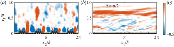
In previous work, swirl strength signed by the out-of-plane vorticity unit vector (Wu & Christensen Reference Wu and Christensen2010) has been used to highlight locations of LMPs and HMPs (Barros & Christensen Reference Barros and Christensen2014; Anderson et al. Reference Anderson, Barros, Christensen and Awasthi2015a). This quantity is useful, as it isolates regions of rotation. For consistency, figure 6 shows signed swirl strength in spanwise– and streamwise–wall-normal planes, where (a1) shows counter-rotating cells associated with downwelling of fluid onto the elements. As expected, visualization in the streamwise–wall-normal plane for this case reveals no heterogeneity, since obliquity has not induced any mean lateral transport. Prior work has focused on large-scale turbulence content within HMPs and LMPs (Awasthi & Anderson Reference Awasthi and Anderson2018), and this work is subsequently not addressed here.
Colour flood contours of time-averaged swirl strength,  $\langle \lambda _{ci} \rangle _t ({\boldsymbol {x}})$ (Wu & Christensen Reference Wu and Christensen2010), signed by the out-of-plane vorticity unit vector,
 $\hat {\boldsymbol {i}}_\omega = \langle \tilde {\omega } \rangle _t / ( \langle \tilde {\omega } \rangle _t : \langle \tilde {\omega } \rangle _t )$. (a,b) Correspond to visualization in the spanwise– and streamwise–wall-normal planes, respectively, with results shown here for case A2a only (see also table 1 for additional case information). The spanwise– (a) and streamwise–wall-normal (b) transects are derived from
 $x_1 = L_1/2$ and
 $x_2 = L_2/2$, respectively.

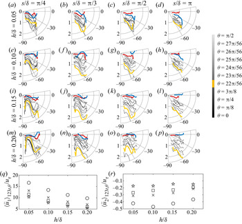
In order to present this effect, figure 7(a–p) shows hodographs of streamwise and spanwise velocity for all table 1 cases. The hodographs are recovered from the centre of the domain and shown against wall-normal elevation,  $\{ \langle \tilde {u}_1 \rangle _t (L_1/2, L_2/2, x_3)/ \langle \tilde {u}_1 \rangle _{123t,\theta }$,
 $\langle \tilde {u}_2 \rangle _t (L_1/2, L_2/2, x_3)/\langle \tilde {u}_2 \rangle _{123t,\theta } \}$, where the normalizing scales –
 $\langle \tilde {u}_1 \rangle _{123t,\theta }$ and
 $\langle \tilde {u}_2 \rangle _{123t,\theta }$ – are derived from the time- and volume-averaged velocity, and subsequently averaged over the range of obliquity values for each unique value of element height and spacing. This averaging approach is necessary to isolate the influence of element height and spacing on the hodographs; for reference, figure 7(q,r) shows
 $\langle \tilde {u}_1 \rangle _{123t,\theta }$ and
 $\langle \tilde {u}_2 \rangle _{123t,\theta }$, respectively, where the symbol nomenclature has been defined in the figure caption. Upon inspection, it is clear that increasing element height and decreasing
 $\hat {x}_1$-aligned spacing both induce monotonic decreases in
 $\langle \tilde {u}_1 \rangle _{123t,\theta }$. This is physically intuitive evidence of a relative momentum penalty due to relatively ‘more rough’ topographies. Moreover, as the element height and/or spacing increases, the induced
 $\langle \tilde {u}_2 \rangle _{123t,\theta }$ strengthens; there is an exception for the average of cases A1b, B1b, C1b, D1b, E1b, F1b, G1b, H1b, I1b, J1b and K1b, although this is likely the product of a slightly inadequate averaging duration. Normalization by
 $\langle \tilde {u}_1 \rangle _{123t,\theta }$ and
 $\langle \tilde {u}_2 \rangle _{123t,\theta }$ provides a needed normalizing scale to assess the influence of obliquity – in the absence of this normalization,
 $\langle \tilde {u}_1 \rangle _t (L_1/2, L_2/2, x_3) \gg \langle \tilde {u}_2 \rangle _t (L_1/2, L_2/2, x_3)$, which prevented visualization of salient trends.
Hodographs of time-averaged velocity,  $\{\langle \tilde {u}_1 \rangle _t ({\boldsymbol {x}}), \langle \tilde {u}_2 \rangle _t ({\boldsymbol {x}}) \}$, shown at
 $x_1 = L_1/2$ and
 $x_2 = L_2/2$. Left-to-right and top-to-bottom correspond to the directions of increasing spacing and element height, respectively. For perspective, hodograph velocities are normalized by
 $\langle \tilde {u}_1 \rangle _{123t,\theta }$ and
 $\langle \tilde {u}_2 \rangle _{123t,\theta }$, or the average velocity for cases with fixed element height and spacing but variable obliquity; these values are shown in (q,r), respectively. In (a–p), critical obliquity is denoted by the yellow profile, while spanwise-heterogeneous (
 $\theta = 0$) and streamwise-heterogeneous (
 $\theta = {\rm \pi}/2$) cases are denoted by red and blue, respectively. Intermediate obliquity is denoted by thin black lines. In (q,r), symbols correspond to different element spacings:
 $s/\delta = {\rm \pi}$ (circle),
 $s/\delta = {\rm \pi}/2$ (
 $\times$),
 $s/\delta = {\rm \pi}/3$ (square) and
 $s/\delta = {\rm \pi}/4$ (star); this symbolic notation is used hereafter.

Given the preceding comments, it is self-evident that for cases with  $\theta = 0$ and
 ${\rm \pi} /2$, hodographs should manifest as horizontal lines since
 $\langle \tilde {u}_2 \rangle _t (L_1/2, L_2/2, x_3) \approx 0$ (at least above the region where any roughness sublayer effects induce finite spanwise velocity). Inspection of figure 7(a–p) shows that this occurs throughout (red and blue profiles, respectively). Likewise, since
 $\langle \tilde {u}_1 \rangle _{123t,\theta }$ declines with increasing element height and/or smaller values of
 $s/\delta$ (figure 7q), it follows that the magnitude of figure 7(a–p) profiles should decrease from the bottom-left (m) to top-right (d) corner. Recall from § 2.1 (LES code description) that each case is subjected to the same forcing – streamwise pressure gradient equivalent to
 $1$ following normalization – and the code is numerically integrated until a balance between the imposed forcing and opposing stress is attained. As such, the trends presented herein are true momentum penalties and not the consequence of variable normalization
 $u_\tau$. Beyond the profiles for
 $\theta = 0$ and
 ${\rm \pi} /2$, which are entirely expected, it is clear that for increasing obliquity
 $\langle \tilde {u}_2 \rangle _t (L_1/2, L_2/2, x_3)/\langle \tilde {u}_2 \rangle _{123t,\theta }$ gets ‘more negative’ due to flow steering in response to the oblique flow-roughness arrangement (see also figure 4). The magnitude of this continues to increase with increasing obliquity, before an asymptote at the critical obliquity,
 $\theta _c$, is attained (yellow profiles in figure 7a–q); for
 $\theta > \theta _c$, the values of
 $\langle \tilde {u}_2 \rangle _t (L_1/2, L_2/2, x_3)/\langle \tilde {u}_2 \rangle _{123t,\theta }$ rapidly tend towards 0. There are some exceptions to this, for example panels (g,k,o), but note that obliquity varies relatively weakly for cases B to G, and as such, the actual critical obliquity varies only modestly from the value of
 $\theta _c$ nominated a priori via the exercise in § 1.2 based upon
 $\lambda _f$ and
 $\lambda _f^{*}$. For clarity, only the profiles corresponding to
 $\theta = 0$,
 $\theta _c$ and
 ${\rm \pi} /2$ are highlighted, while intermediate cases are shown with thin black lines. This plotting approach enables the influence of increasing
 $\theta$ to be clearly isolated.
As outlined in § 1.2, the critical obliquity is a product of successive element sheltering: the IBL-like flow response persists across  $\theta$ – even as a significant value of
 $\langle \tilde {u}_2 \rangle _t (L_1/2, L_2/2, x_3)$ begins to accumulate – before abruptly collapsing at the critical obliquity. Following this, successive element shelterings preclude formation of new IBLs from the roughness sublayer, and instead the elements behave as a quasi-streamwise-aligned strip of elevated drag, thereby sustaining formation of quasi-streamwise-aligned counter-rotating secondary cells (figure 1 and Anderson et al. Reference Anderson, Barros, Christensen and Awasthi2015a).
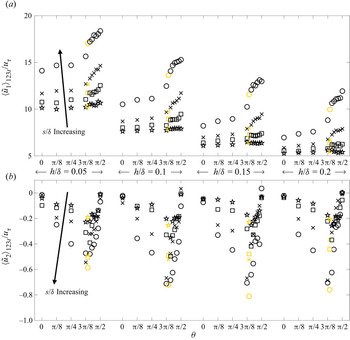
In a further effort to consolidate the results of the LES cases summarized in table 1, and to provide further insight into bulk dynamical trends associated with the parametric variation assessed herein, figure 8(a,b) shows time- and volume-averaged streamwise and spanwise velocities, respectively. The datapoints are grouped based upon the element height (left-to-right), the symbol nomenclature is defined in the figure 7(q,r) caption and obliquity angle increases within the height subsets in figure 8. Unlike figure 7(a–p), for which the velocities are normalized in order to visualize underlying trends in the profiles, ‘pre-normalized’ velocity is not shown in figure 8. For the smallest spacing,  $s/\delta = {\rm \pi}/4 \approx 0.781$, which renders the complex roughness distribution a ‘roughness’, as per Yang & Anderson (Reference Yang and Anderson2017). In this regime, element-driven disturbances are confined to the roughness sublayer by virtue of a relatively smaller spacing between adjacent rows (Anderson et al. Reference Anderson, Barros, Christensen and Awasthi2015a; Anderson Reference Anderson2019), which explains the relatively weak dependence of
 $\langle \tilde {u}_1 \rangle _{123t}$ on
 $\theta$ (a). Likewise, since element-driven disturbances are present in the roughness sublayer – and due to flow asymmetry owing to flow-heterogeneity obliquity – finite values of
 $\langle \tilde {u}_2 \rangle _{123t}$ are observed on figure 8(b). However, the magnitude of
 $\langle \tilde {u}_2 \rangle _{123t}$ for
 $s/\delta = {\rm \pi}/4$ is smallest.
Time- and volume-averaged streamwise (a) and spanwise (b) velocities for all table 1 cases, displayed against obliquity (abscissa) and grouped based on element height (middle annotation). Critical obliquity denoted with yellow symbols; direction of increasing spacing annotated.

For the relatively larger spacing of  $s/\delta = {\rm \pi}/3 \approx 1$, the surfaces are within the ‘Intermediate’ regime (Yang & Anderson Reference Yang and Anderson2017), and larger-scale flow heterogeneities emerge within the flow. For
 $\theta = 0$ and
 ${\rm \pi} /2$, this would manifest as relatively larger blending elevation (Bou-Zeid et al. Reference Bou-Zeid, Meneveau and Parlange2004) or in the form of
 $\delta$-scale counter-rotating secondary cells, respectively, while for oblique alignments the flow response would exhibit some resemblance to both. For this relatively larger spacing, a pronounced rise in
 $\langle \tilde {u}_1 \rangle _{123t}$ occurs at
 $\theta \gtrsim 3 {\rm \pi}/8$ – the critical obliquity – beyond which the variation in
 $\langle \tilde {u}_1 \rangle _{123t}$ against
 $\theta$ subsequently steepens. This pattern is consistent across the values of height and spacing considered, and can be readily understood as a consequence of successive element shelterings. As established in § 1.2, the critical obliquity corresponds to the value at which successive element shelterings begin: for
 $\theta \gtrsim \theta _c$, the aero-/hydrodynamic signature of the rough surfaces rapidly declines, which manifests itself here in the non-monotonic variation in
 $\langle \tilde {u}_1 \rangle _{123t}$ with
 $\theta$. Similarly, for relatively larger
 $s/\delta$,
 $\langle \tilde {u}_2 \rangle _{123t}$ exhibits a pronounced pattern of strengthening – as flow steering against the oblique heterogeneity induces stronger lateral transport – followed by a dramatic collapse towards
 $\langle \tilde {u}_2 \rangle _{123t} \approx 0$. As per figure 7(a–p), this turning point in
 $\langle \tilde {u}_2 \rangle _{123t}$ against
 $\theta$ corresponds precisely to the critical obliquity. At this value, successive element shelterings begin to preclude the formation of new internal boundary layers, and the surface subsequently behaves as a distributed ‘strip’ of relatively elevated drag that provides sustenance for quasi-streamwise-aligned counter-rotating secondary cells.
3.2. Prognostic roughness model
Since oblique flow-roughness arrangements are expected to be the norm – not the exception – in flow systems of practical importance, it is worthwhile considering the implications of the preceding results for prognostic roughness modelling. Such models are generally predicated upon one or more statistical moment of the surface (Flack & Schultz Reference Flack and Schultz2010; Zhu et al. Reference Zhu, Iungo, Leonardi and Anderson2016), foremost among them being the frontal- and plan-area indices (Raupach Reference Raupach1992; Yang et al. Reference Yang, Sadique, Mittal and Meneveau2016) ((1.1), (1.2) and (1.5)), and height root-mean-square,  $\sigma _{h^{\prime }} = (\langle h^{2} \rangle _{12} - \langle h \rangle _{12}^{2})^{1/2}$ (Zagarola & Smits Reference Zagarola and Smits1998). In fact, in a recent article addressing obliquity and roughness modelling, Anderson (Reference Anderson2020) reviewed these topics and proposed generalization to the standard model based on
 $\sigma _{h^{\prime }}$
 \begin{equation} z_{0,{Eff.}}^{1} = \alpha_1 \sigma_{h'(\boldsymbol{x})}, \end{equation}
where  $\alpha _1 \sim {O}(10^{-1})$ is a constant of proportionality evaluated a posteriori. There are a great many newer roughness models that provide improved generality (Flack & Schultz Reference Flack and Schultz2010; Zhu et al. Reference Zhu, Iungo, Leonardi and Anderson2016; Zhu & Anderson Reference Zhu and Anderson2018), but none are generalized for obliquity. To this extent, (3.1) is helpful in terms of establishing a comparative benchmark. We stress once more that (3.1) by no means represents the state-of-the-art in roughness modelling, and we direct interested readers to more-recent literature in this area (Flack & Schultz Reference Flack and Schultz2010). Nevertheless, since contemporary roughness models are not generalized for obliquity, comparison against prediction from any benchmark model will illustrate the same intrinsic shortcoming. For the oblique surfaces considered in this article, it is self-evident that
 $\sigma _{h^{\prime }}$ exhibits no dependence on obliquity angle. The value of
 $\sigma _{h^{\prime }}$ is strongly dependent upon element height and
 $\hat {x}_1$-aligned spacing, as per figure 9(a), but failure to capture the influence of
 $\theta$ automatically prevents singular dependence of roughness length on
 $\sigma _{h^{\prime }}$, as per (3.1). Likewise,
 $\lambda _p$ (1.5) is strongly dependent on the
 $\hat {x}_1$-aligned spacing (figure 9b), but
 $\lambda _p$ does not capture variable obliquity. As discussed in § 1.2,
 $\lambda _f$ and
 $\lambda _f^{*}$ do vary with obliquity for
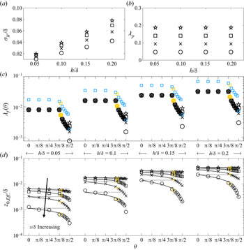
 $\theta > \theta _c$, where the latter is the frontal-area index compensated for successive element shelterings (Raupach Reference Raupach1992; Yang et al. Reference Yang, Sadique, Mittal and Meneveau2016). Figure 9(c) shows
 $\lambda _f$ (black symbols) and
 $\lambda _f^{*}$ (blue symbols) for the cases considered herein, where the symbols for both are yellow at the critical obliquity. As noted,
 $\lambda _f$ and
 $\lambda _f^{*}$ are insensitive to
 $\theta$ for
 $\theta < \theta _c$ (see also figures 2 and 3), before suddenly declining for
 $\theta \geqslant \theta _c$ due to successive element shelterings. Both parameters respond to changing element height, as expected, and also display
 $s/\delta$ dependence for
 $\theta = {\rm \pi}/2$; for all
 $\theta < {\rm \pi}/2$,
 $\lambda _f$ and
 $\lambda _f^{*}$ cannot respond to
 $s/\delta$ by virtue of the periodic boundaries imposed during construction of the surfaces (see also § 2.2). For a relatively more narrow parametric range, Anderson (Reference Anderson2020) proposed a roughness model based on
 $\sigma _{h^{\prime }}$ and
 $\lambda _f$,
 \begin{equation} z_{0,{Eff.}}^{2} = \alpha_2 \sigma_{h'(\boldsymbol{x})} \lambda_f[1-\alpha_3 \exp(\alpha_4 \theta)], \end{equation}
where  $\alpha _2$,
 $\alpha _3$ and
 $\alpha _4$ are empirical proportionality constants recovered a posteriori (discussion to follow).
Summary of geometric and aerodynamic attributes for rough surface cases considered in this article, where (a) shows height root-mean-square,  $\sigma _{h^{\prime }} = (\langle h^{2} \rangle - \langle h \rangle ^{2})^{1/2}$, (b) shows plan-area index (1.5) and (c) shows frontal-area index (black symbols; (1.1)) and compensated frontal-area index (blue symbols; (1.2)). The values of
 $\sigma _{h^{\prime }}$ and
 $\lambda _p$ do not change with obliquity, and are instead displayed against element height;
 $\lambda _f$ and
 $\lambda _f^{*}$ change with obliquity and height, while spacing effects are apparent only once a definitively spanwise-heterogeneous surface is attained (
 $\theta = {\rm \pi}/2$). (d) Shows effective roughness lengths recovered a posteriori for all table 1 cases, plotted against obliquity angle (abscissa) and grouped based upon element height (annotation at top). Solid grey and black profiles correspond to predictions from (3.1) and (3.2), respectively, where the latter is compensated for obliquity. Yellow symbols denote critical obliquity (see also figures 2 and 3).

The effective roughness length,  $z_{0,{Eff.}}$, was recovered a posteriori for all table 1 cases. The value of
 $z_{0,\mathrm {Eff.}}$ was recovered via application of a least-squares fit of a logarithmic profile to the plane- and time-averaged streamwise velocity for each of the table 1 cases. The results are summarized in figure 9(d), where the symbol nomenclature was defined in the figure 7 caption and the direction of
 $s/\delta$ increasing has been annotated, for perspective. Since
 $z_{0,{Eff.}}$ is a consequence of the flow statistics already presented, the results vary in a consistent manner. For increasing element height, the effective roughness length monotonically increases as the surface momentum penalty increases. Likewise, as the
 $\hat {x}_1$-normal spacing between successive rows of elements increases – corresponding to a declining number of elements and lower values of
 $\sigma _{h^{\prime }}$ (figure 9a) – the effective roughness length also declines. The results in figure 9(d) demonstrate that
 $z_{0,{Eff.}}$ responds monotonically to variability in
 $h/\delta$ and
 $s/\delta$; the response to obliquity is intrinsically dependent upon successive element shelterings.
In figure 9(d), the value of  $z_{0,{Eff.}}$ at the critical obliquity is denoted by yellow symbols, for perspective and as per preceding results; figure 9(d) shows that these ‘critical’ values represent a dramatic turning point in the dependence upon
 $\theta$ (note that the ordinate is shown in logarithmic scale). The results are consistent with figures 7 and 8: for
 $0 < \theta \lesssim \theta _c$, IBL-like flow processes persist, but oblique alignments incur a relatively lesser aero-/hydrodynamic penalty. The value of
 $z_{0,{Eff.}}$ declines substantially faster following the critical obliquity, as successive element shelterings reduce the bulk aero-/hydrodynamic signature of these surfaces. As per figure 8(a), for the smallest
 $\hat {x}_1$-normal spacing,
 $s/\delta = {\rm \pi}/4 \approx 0.78$, the surfaces more closely resemble a ‘roughness’, for which element-driven effects are confined within the roughness sublayer. Evidence of this is apparent in the relatively weak variation of
 $z_{0,{Eff.}}$ with
 $\theta$.
The efficacy of (3.1) and (3.2) over the very large parametric range considered is herein assessed. The solid grey profiles in figure 9(d) correspond to (3.1) ( $\alpha _1 = 0.12$), where singular dependence on
 $\sigma _{h^{\prime }}$ precludes any dependence on
 $\theta$ (see also figure 9(a) and accompanying discussion). For
 $\theta = 0$, (3.1) closely agrees with the a posteriori data, while for
 $0 < \theta \lesssim \theta _c$, the agreement is reasonable; note that (3.1) is relatively accurate for all
 $\theta$ for the case of
 $s/\delta = {\rm \pi}/4 \approx 0.78$, since this spacing more closely resembles a roughness. Following the critical obliquity, however, (3.1) predictions significantly diverge from the LES data, where it is once again emphasized that the figure 9(d) ordinate is in logarithmic scale.
The solid black profiles in figure 9(d) correspond to (3.2) ( $\alpha _2 = 0.95$,
 $\alpha _3 = 0.1$ and
 $\alpha _4 = 1.35$). Results demonstrate that, for the vast parametric range considered herein – encompassing element height,
 $\hat {x}_1$-normal spacing and obliquity – (3.2) is able to predict the bulk roughness length with fidelity. This prognostic capability is derived from simultaneous dependence on
 $\sigma _{h^{\prime }}$ and
 $\lambda _f$, where the former acts as an amplitude while the latter captures abrupt variation for
 $\theta \gtrsim \theta _c$ (figure 9c).
4. Concluding remarks
Canonical high- $Re_\tau$ wall-sheared turbulent flows are composed of a viscous-affected near-wall region and an inertial outer layer, where the latter is occupied by large (
 $\delta$) scale coherent structures. A homogeneous distribution of relatively low-amplitude roughness elements ablates the viscous layer, but inertial-layer structures are dynamically and structurally unchanged (outer-layer similarity). Heterogeneous distributions of low-amplitude roughness, however, can entirely disrupt the outer-layer flow with the emergence of roughness-driven Reynolds-averaged wakes and secondary flows. LES has been used to perform a large-scale parametric study to capture bulk flow response to variation in element height, spacing between adjacent rows of elements and flow-roughness obliquity. The study builds on prior work (Anderson Reference Anderson2012), but is far more expansive in scope. In prior work (Anderson Reference Anderson2020) and in the present article, we find that time- and volume-averaged streamwise and spanwise velocity datapoints for each simulation exhibit a pronounced non-monotonic pattern. As
 $\theta$ is increased from 0 (streamwise heterogeneity),
 $\langle \tilde {u}_1 \rangle _{123t}$ and
 $\langle \tilde {u}_2 \rangle _{123t}$ slowly increase and decrease, respectively. At a specific value of obliquity – termed the critical obliquity – the aforementioned trends abruptly change, with
 $\langle \tilde {u}_1 \rangle _{123t}$ rising much faster while
 $\langle \tilde {u}_2 \rangle _{123t}$ tends to 0. This pattern marks the persistence of IBL-like flow processes, which necessarily collapse at the critical obliquity and mark the emergence of quasi-streamwise-aligned Reynolds-averaged secondary cells. This pattern repeats with changing element height and changing element spacing. We demonstrate that the pattern itself is a consequence of successive element shelterings at the critical obliquity, which can be readily understood when interpreted via the ‘observer’ view of the roughness: for
 $\theta \gtrsim \theta _c$, successive element shelterings fundamentally alter the flow response by precluding the formation of new IBLs; instead, the distribution of elements manifests as a quasi-streamwise-aligned distribution of elevated surface stress, which sustains secondary cells. The implications of this for prognostic roughness modelling were reviewed, and we demonstrate efficacy of a model recently proposed by Anderson (Reference Anderson2020).
A series of additional exercises can be envisioned. For example: Given the clear importance of element sheltering, what is the flow response when non-cuboid elements are used? We found that the wake sheltering angle was relatively small (Raupach Reference Raupach1992; Yang et al. Reference Yang, Sadique, Mittal and Meneveau2016), and as a result,  $\lambda _f$ and
 $\lambda _f^{*}$ exhibited similar functional forms. If we had used conical, pyramid or spheroid elements, for example, how would the results differ? This and other complementary questions are deserving of further attention.
Acknowledgements
Special thanks to K.T. Christensen for suggesting interpretation of the results in terms of frontal-area index.
Funding
This work was supported by the U.S. Air Force Office of Scientific Research, Grant no. FA9550-19-1-0134 (W.A.). Computational resources were provided by the Texas Advanced Computing Center at the University of Texas.
Declaration of interests
The authors report no conflict of interest.