1. INTRODUCTION
Currently, apart from the full global coverage satellite systems (GPS, GLONASS and BDS-3), all the regional and new navigation satellite systems, namely, BDS-2, quasi-zenith satellite system (QZSS), IRNSS and Galileo, can provide at least two frequencies and have the ability to offer space-based positioning, navigation and timing (PNT) services (Gao et al., Reference Gao, Gao and Pan2017b; Zhang et al., Reference Zhang, Chen and Yuan2019). The joint use of multi-frequency and multi-system global navigation satellite systems (GNSSs) to improve positioning accuracy and reliability has been widely applied in many fields (Zhang et al., Reference Zhang, Teunissen and Yuan2017; Shang et al., Reference Shang, Gao, Pan, Meng and Gao2019). However, for multi-GNSS double-differenced relative positioning, the traditional intra-system model, which chooses a pivot satellite for each system, cannot provide precise positioning in complex environments as it is unable to form a double-difference observation equation. In order to increase the amount of redundant information and improve the positioning accuracy, especially for applications in complex environments, an inter-system model has been proposed that needs only one pivot satellite (Wu et al., Reference Wu, Zhang, Liu, Ni and Yu2017). Compared with the intra-system model, the inter-system model not only introduces at least one more redundancy, but also ensures positioning when very few satellites are visible for a single system (Julien et al., Reference Julien, Alves, Cannon and Zhang2003). The key to developing the inter-system model is the handling of the differential inter-system biases (DISBs) among systems (Gao et al., Reference Gao, Gao, Pan, Meng and Xia2017a, Reference Gao, Meng, Gao, Pan and Wang2018).
For phase DISBs (PDISBs) with overlapping frequencies, the integer part of the PDISB can be absorbed into the integer ambiguities and does not need further treatment. However, the fractional part of PDISBs (F-PDISBs) will influence the integer feature of the inter-system double-difference ambiguities. When introducing the F-PDISB parameter to the double-difference observation model directly, the equation cannot be solved due to the rank deficiency. To tackle this problem, Odijk and Teunissen (Reference Odijk and Teunissen2013a, Reference Odijk and Teunissen2013b) suggested choosing pivot satellites for GPS and Galileo separately. In this case, for the Galileo pivot satellite, it will compose the double difference with the GPS pivot satellite. For other Galileo satellites the ambiguities relative to the GPS pivot satellite originally can be reintegrated into ambiguities relative to the Galileo pivot satellite in the inter-system model, to obtain the full-ranked model. Paziewski and Wielgosz (Reference Paziewski and Wielgosz2015) assigned a priori values for the F-PDISBs to remove rank deficiency between F-PDISBs and ambiguity. Since then, many researchers have studied the inter-system model for overlapping frequencies (BDS B2 and Galileo E5b, QZSS L1 and GPS L1, etc.) and their findings indicate that the code DISBs and PDISBs are zero for baselines made up of the same type of receivers (Odolinski et al., Reference Odolinski, Teunissen and Odijk2014, Reference Odolinski, Teunissen and Odijk2015; Nadarajah et al., Reference Nadarajah, Khodabandeh and Teunissen2015; Odolinski and Teunissen, Reference Odolinski and Teunissen2016; Odijk et al., Reference Odijk, Nadarajah, Zaminpardaz and Teunissen2017; Paziewski and Wielgosz, Reference Paziewski and Wielgosz2017). For baselines made up of the different types of receivers, the DISBs are stable and can be corrected in advance. Therefore, it is easy to compose the inter-system model to improve positioning accuracy for short (<15 km) and medium–long (>15 km) baseline real time kinematic (RTK) positioning. Based on these characteristics, Tian et al. (Reference Tian, Ge, Neitzel and Zhu2017) introduced a particle filter to calculate the DISBs and proposed a real-time DISB computing method.
For the model of different frequency inter-system double differencing, because of the influence of the pivot satellite single-difference ambiguity, it is a challenge to calculate the F-PDISBs and obtain the integer inter-system double-difference ambiguities. Li et al. (Reference Li, Wu, Zhao and Tian2017) suggested using the linear combinations of multi-frequency carrier phase to decrease the effect of different frequencies on the ambiguity resolution. However, it is impossible for a device collecting only single-frequency observations to gather multi-frequency observations. Gao et al. (Reference Gao, Gao, Pan, Meng and Xia2017a, Reference Gao, Meng, Gao, Pan and Wang2018) proposed a combined GPS and BDS single-frequency continuous RTK positioning model through real-time estimation of DISBs. They found that although a single-difference ambiguity with a wavelength of a few millimetres has to be taken into account along with the F-PDISBs, for the baselines with the same receiver types and some with different receiver types, the F-PDISBs could still be verified as relatively stable within several days. Because the method needs real-time calculation of F-PDISBs, however, the computational efficiency is unsatisfactory. According to the research mentioned above, for the non-overlapping frequencies, once the initial value of F-PDISBs is obtained, the F-PDISBs can remain stable and consistent so that an inter-system model for the non-overlapping frequencies system can be achieved. In this study, after analysing the stability of F-PDISBs, the particle filter was utilised to calculate the initial value of F-PDISBs. In the particle filter, the F-PDISB samples are generated first, and then they are treated as known F-PDISB values in double-differencing ambiguity resolution. The F-PDISBs samples that have the closest values to the truth can recover the integer nature of the inter-system double-differencing ambiguities and result in the largest ratio values. After the particle weights are updated according to the ratio values in the particle filtering, the F-DISPBs can be successfully estimated according to the weighted particles.
The rest of this paper is organised as follows: In Section 2, the intra-system and inter-system observation models are introduced in detail. In Section 3, analysis of the stability of GPS L1-BDS B1, GPS L2-Galileo E5a, code DISBs and F-PDISBs is presented. Section 4, investigates the relationship between ratio and F-PDISBs, and proposes a particle filter-based F-PDISB estimation method. Section 5 presents analysis of the improvement of the inter-system differencing model over the intra-system differencing model with various simulated satellite visibilities. Finally, the research findings are summarised.
2. INTRA-SYSTEM AND INTER-SYSTEM OBSREVATION MODELS
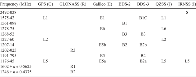
As shown in Table 1 (Quasi-Zenith Satellite System (QZSS), 2019; Yang et al., Reference Yang, Gao, Guo, Mao and Yang2019), in multi-GNSS positioning, a large number of GNSS signals have non-overlapping frequencies, for example, the BDS-2 B1 and GPS L1, or the GPS L2 and Galileo E5a. This section discusses the intra-system and inter-system models for these non-overlapping frequency systems.
Signal frequencies of GNSS.

Note: n = −7, −6, −5 … 6, the channel numbers of GLONASS satellites.
2.1. Un-differenced code and phase observation models
For a clearer explanation, these sections commence with the un-differenced (UD) code and phase observations of these systems. First, the UD code and phase observation models in units of metres for GPS can be expressed as follows:
 $$\left\{ {\begin{array}{@{}l@{}} L_{a,i}^{g_s } =\rho_{a,i}^{g_s } +c(dt_a -dt^{g_s })-I_{a,i}^{g_s } +T_{a,i}^{g_s } +\lambda_{g,i} (b_{a,i}^g +\varphi_{a,i}^g -b_i^{g_s } -\varphi_i^{g_s } +N_{a,i}^{g_s } )+\varepsilon_{a,i}^{g_s } \\[6pt] P_{a,i}^{g_s } =\rho_{a,i}^{g_s } +c(dt_a -dt^{g_s })-I_{a,i}^{g_s } +T_{a,i}^{g_s } +d_{a,i}^g -d_i^{g_s } +e_{a,i}^{g_s } \end{array}} \right.$$
where L is the phase observation and P is code observation, the subscript a represents the pivot receiver, i = 1, …, f are the GPS frequencies and  $g_{s}=g_{1}, \; \ldots, \; g_{m}$ are the GPS satellites, m is the number of GPS satellite, c is the speed of light, ρ is the distance between satellite and receiver, λg, i is the wavelength of the GPS, dt a is the receiver clock error, dt gs is the GPS satellite clock error, and I and T are the ionospheric and tropospheric delays, respectively.
 $b_{a, i}^{g} $ and
 $b_{i}^{g_{s} } $ stand for the hardware phase delays in the receiver and satellite, respectively.
 $\varphi _{a, i}^{g} $ and
 $\varphi _{i}^{g_{s} } $ are the initial phase in the receiver and satellite, respectively.
 $N_{a, i}^{g_{s} } $ is the integer phase ambiguity.
 $d_{a, i}^{g} $ and
 $d_{i}^{g_{s} }$ stand for the hardware code delay in the receiver and satellite, respectively. ɛ and e are the measurement noises for phase and code observations, respectively.
Second, the UD code and phase observation models for other CDMA systems (BDS, Galileo, QZSS, IRNSS) can be derived similarly. It is worth noting that because of the different time systems used for GPS and these systems, a time offset (*GTO) must be employed to convert these systems' time to GPS time. Hence, the following model for these systems can be formed:
 $$\left\{ {\begin{array}{@{}l@{}} L_{a,j}^{\ast_s } =\rho_{a,j}^{\ast_s } +c(dt_a -dt^{\ast_s })-d_{\ast{\rm GTO}} -I_{a,j}^{\ast_s } +T_{a,j}^{\ast_s }\\[3pt] +\,\lambda_{\ast, j} (b_{a,j}^\ast +\varphi_{a,j}^\ast -b_i^{\ast_s } -\varphi_i^{\ast_s } +N_{a,j}^{\ast_s } )+\varepsilon_{a,j}^{\ast_s } \\ P_{a,j}^{\ast_s } =\rho_{a,j}^{\ast_s } +c(dt_a -dt^{\ast_s })-d_{\ast {\rm GTO}} -I_{a,j}^{\ast_s } +T_{a,j}^{\ast_s } +d_{a,j}^\ast -d_j^{\ast_s } +e_{a,j}^{\ast_s } \end{array}} \right.$$
where symbol * is B for BDS, E for Galileo, Q for QZSS and I for IRNSS, j = 1, …, f are the frequencies of *,  $d_{\ast {\rm GTO}}$ is the *-to-GPS time offset. The other symbols of the parameters are similar to GPS and are omitted for simplicity.
2.2. Single differencing models
Based on the UD code and phase observation models, the short baseline between receiver (for pivot receiver ‘a’ and rover receiver ‘b’) single differencing models can be derived as Equations (3) and (4), respectively, in which the differential tropospheric and ionospheric biases, the  $d_{\ast {\rm GTO}}$, as well as the other satellite-specific biases will be eliminated.
 $$\begin{align} &\left\{ {\begin{array}{@{}l@{}} \Delta L_{ab,i}^{g_s } =\Delta \rho_{ab,i}^{g_s } +\Delta dt_{ab} +\lambda_{g,i} (\Delta b_{ab,i}^g +\Delta \varphi_{ab,i}^g +\Delta N_{ab,i}^{g_s })+\varepsilon_{ab,i}^{g_s } \\ \Delta p_{ab,i}^{g_s } =\Delta \rho_{ab,i}^{g_s } +\Delta dt_{ab} +\Delta d_{ab,i}^g +e_{ab,i}^{g_s } \end{array}} \right.\end{align}$$
 $$\begin{align} &\left\{ {\begin{array}{@{}l@{}} \Delta L_{ab,j}^{\ast_s } =\Delta \rho_{ab,j}^{\ast_s } +\Delta dt_{ab} +\lambda_{\ast, j} (\Delta b_{ab,j}^\ast +\Delta \varphi_{ab,j}^\ast +\Delta N_{ab,j}^{\ast_s } )+\varepsilon_{ab,j}^{\ast_s } \\ \Delta P_{ab,j}^{\ast_s } =\Delta \rho_{ab,j}^{\ast_s } +\Delta dt_{ab} +\Delta d_{ab,j}^\ast +e_{ab,j}^{\ast_s } \end{array}} \right. \end{align}$$
2.3. Intra-system observation models
Assuming that in epoch t 1 satellites g 1, *1 are chosen as pivot satellites and form double differencing for each system, the receiver-dependent biases can be eliminated and thus the classical intra-system model can be formed as:
 $$\left\{ {\begin{array}{@{}l@{}} \nabla \Delta L_{ab,i}^{g_1 g_2 } =\nabla \Delta \rho_{ab,i}^{g_1 g_2 } +\lambda_{g,i} \nabla \Delta N_{ab,i}^{g_1 g_2 } )+\varepsilon_{ab,i}^{g_1g_2 } \\[5pt] \nabla \Delta P_{ab,i}^{g_1 g_2 } =\nabla \Delta \rho_{ab,i}^{g_1 g_2 }+e_{ab,i}^{g_1 g_2 } \\[5pt] \nabla \Delta L_{ab,i}^{g_1 g_3 } =\nabla \Delta \rho_{ab,i}^{g_1 g_3 }+\lambda_{g,i} \nabla \Delta N_{ab,i}^{g_1 g_3 } )+\varepsilon_{ab,i}^{g_1g_3 } \\[5pt] \nabla \Delta P_{ab,i}^{g_1 g_3 } =\nabla \Delta \rho_{ab,i}^{g_1 g_3 }+e_{ab,i}^{g_1 g_3 } \\[5pt] \vdots \\[5pt] \nabla \Delta L_{ab,j}^{\ast_1 \ast_2 } =\nabla \Delta \rho_{ab,j}^{\ast_1 \ast_2 } +\lambda_{\ast, j} \nabla \Delta N_{ab}^{\ast_1 \ast_2 })+\varepsilon_{ab,j}^{\ast_1 \ast_2 } \\[5pt] \nabla \Delta P_{ab,j}^{\ast_1 \ast_2 } =\nabla \Delta \rho_{ab,j}^{\ast_1 \ast_2 } +e_{ab,j}^{\ast_1 \ast_2 } \\[5pt] \nabla \Delta L_{ab,j}^{\ast_1 \ast_3 } =\nabla \Delta \rho_{ab,j}^{\ast_1 \ast_3 } +\lambda_{\ast, j} \nabla \Delta N_{ab}^{\ast_1 \ast_3 })+\varepsilon_{ab,j}^{\ast_1 \ast_3 } \\[5pt] \nabla \Delta P_{ab,j}^{\ast_1 \ast_3 } =\nabla \Delta \rho_{ab,j}^{\ast_1 \ast_3 } +e_{ab,j}^{\ast_1 \ast_3 } \\[5pt] \vdots \end{array}} \right.$$
2.4. Inter-system observation models
Choosing the GPS satellite g 1 as the pivot satellite, the inter-system model can be built similarly. However, the hardware delays and the initial phase cannot be eliminated, in addition, because  $\lambda _{g, i} \ne \lambda _{\ast, 1}$, so the single-difference ambiguities cannot be integrated. Therefore, after simple recombination, we derive Equation (6) in which the inter-system double-difference ambiguities have integer features.
 $$\begin{align} &\left\{ {\begin{array}{@{}l@{}} \nabla \Delta L_{ab,ij}^{g_1 \ast_s } =\nabla \Delta \rho_{ab,ij}^{g_1 \ast_s } +\lambda_{\ast, j} \nabla \Delta N_{ab,ij}^{g_1 \ast_s } +\lambda_{\ast, j} B_{ab,ij}^{g_\ast } +\varepsilon_{ab,ij}^{g_1 \ast_s }\\[5pt] \nabla \Delta P_{ab,ij}^{g_1 \ast_s } =\nabla \Delta \rho_{ab,ij}^{g_1 \ast_s } +\nabla \Delta d_{ab,ij}^{g_\ast } +e_{ab,ij}^{g_1 \ast_s } \end{array}} \right.\end{align}$$
 $$\begin{align} & B_{ab,ij}^{g\ast } =\frac{1}{\lambda _{\ast, j} }[ {( {\lambda_{\ast, j} -\lambda_{g,i} } ) \nabla \Delta N_{ab}^{g_1 } +\lambda_{\ast, j} ( {b_{ab}^\ast +\varphi_{ab}^\ast } ) -\lambda_{g,i} ( {b_{ab}^g +\varphi_{ab}^g } ) } ] \end{align}$$
As it is impossible to estimate the F-PDISBs parameters, the inter-system double-difference ambiguities and the single-difference ambiguity of the GPS pivot satellite simultaneously, however, the mixed observation contains a rank deficiency. In order to solve this problem, the pivot satellites for GPS and * are selected separately. The ambiguities relative to the GPS pivot satellite originally can be reintegrated into ambiguities relative to the * pivot satellite in the inter-system model so that we can change the form of the double-difference ambiguity as follows
 $$\begin{align} \nabla \Delta N_{ab,ij}^{g_1 \ast _s } =( {\nabla \Delta N_{ab,j}^{\ast s} -\nabla \Delta N_{ab,j}^{\ast 1} } ) +( {\nabla \Delta N_{ab,j}^{\ast 1} -\nabla \Delta N_{ab,j}^{g_1 } } ) =\nabla \Delta N_{ab,j}^{\ast 1\ast s} -\nabla \Delta N_{ab,ij}^{g_1 \ast _1 } \end{align}$$
Then the single-difference ambiguities of the GPS pivot satellite and the ambiguities between GPS and * pivot satellite can join the F-PDISBs term. Therefore, we can get the full-rank inter-system model.
 $$\left\{ {\begin{array}{@{}l@{}} \nabla \Delta L_{ab,ij}^{g_1 \ast_s } =\nabla \Delta \rho_{ab,ij}^{g_1 \ast_s } +\lambda_{\ast, j} \nabla \Delta N_{ab,j}^{\ast 1\ast s} +\lambda_{\ast, j} \mbox{PDISB}_{ab,ij}^{g\ast } +\varepsilon_{ab,ij}^{g_1 \ast_s} \\[5pt] \nabla \Delta p_{ab,ij}^{g_1 \ast_s } =\nabla \Delta \rho_{ab,ij}^{g_1 \ast_s } +\nabla \Delta d_{ab,ij}^{g\ast } +e_{ab,ij}^{g_1 \ast_s } \\ \end{array}} \right.$$
where
 $$\begin{align} \mbox{PDISB}(t_1 )_{ab,ij}^{g\ast } &=B_{ab,ij}^{g\ast } +\nabla \Delta N_{ab,ij}^{g_1 \ast _1 }\nonumber\\[4pt] &=\frac{1}{\lambda _{\ast, j} }[ {( {\lambda_{\ast, j} -\lambda_{g,i} } ) \nabla \Delta N_{ab,i}^{g_1 } +\lambda_{\ast, j} ( {b_{ab,j}^\ast +\varphi_{ab,j}^\ast } ) -\lambda_{g,i} ( {b_{ab,i}^g +\varphi_{ab,i}^g } ) } ] \nonumber\\[4pt] &\quad +\nabla \Delta N_{ab,ij}^{g_1 \ast _1 } \end{align}$$
From Equation (10) we can see that the newly combined PDISBs not only include the single-difference ambiguity of the GPS pivot satellite, but also the double-difference ambiguity of the pivot satellite of * and GPS. Assume that in epoch t 2 the GPS pivot satellite changed to g 2, then the PDISB can be expressed as in Equation (11). In order to maintain the F-PDISBs, we added the ambiguity between the two GPS pivot satellites to Equation (11) as shown in Equation (12). It can be seen from Equation (12) that when the GPS pivot satellite changes from g 1 to g 2, the F-PDISBs are the same.
 $$\begin{align} \mbox{PDISB}_{ab,ij}^{g\ast } (t_2 )&=\frac{1}{\lambda _{\ast, j} }[ {( {\lambda_{\ast, j} -\lambda_{g,i} } ) \nabla \Delta N_{ab,i}^{g_2 } +\lambda_{\ast, j} ( {b_{ab,j}^\ast +\varphi_{ab,j}^\ast } ) -\lambda_{g,i} ( {b_{ab,i}^g +\varphi_{ab,ij}^g } ) } ] \nonumber\\[4pt] &\quad+\nabla \Delta N_{ab,ij}^{g_2 \ast _1 } \end{align}$$
 $$\begin{align} \delta \mbox{PDISB}_{ab,ij}^{g\ast } (t_1 t_2 )&=\mbox{PDISB}_{ab,ij}^{g\ast } (t_2 )-\mbox{PDISB}_{ab,ij}^{g\ast } (t_1 )=\frac{\lambda _{g,i} }{\lambda _{c,j} }\nabla \Delta N_{ab,i}^{g_2 g_1 } \end{align}$$
Assume that in epoch t 2 the * pivot satellite changed to *2, then the PDISBs can be expressed as Equation (13). In order to maintain the PDISBs, we added the ambiguity between the two * pivot satellites to Equation (13), as Equation (14) shows. It can be seen from Equation (13) that when the * pivot satellite changes, the F-PDISBs remains the same.
 $$\begin{align} \mbox{PDISB}_{ab,ij}^{g\ast } (t_2 )&=\frac{1}{\lambda _{\ast, j} }[ {( {\lambda_{\ast, j} -\lambda_{g,i} } ) \nabla \Delta N_{ab,i}^{g_2 } +\lambda_{\ast, j} ( {b_{ab,j}^\ast +\varphi_{ab,j}^\ast } ) -\lambda_{g,i} ( {b_{ab,i}^g +\varphi_{ab,i}^g } ) } ] \nonumber\\ &\quad +\nabla \Delta N_{ab,ij}^{g_2 \ast _2 } \end{align}$$
 $$\begin{align} \delta \mbox{PDISB}_{ab,ij}^{g\ast } ( {t_2 t_3 })&=\mbox{PDISB}_{ab,ij}^{g\ast } ( {t_3 } )-\mbox{PDISB}_{ab,ij}^{g\ast } ( {t_2 })=\nabla \Delta N_{ab,j}^{\ast 2\ast 1} \end{align}$$
When the pivot satellite of GPS and * change, the integer and fractional parts of the PDISBs parameter can maintain stability by parameter conversion, and the integer part can be absorbed by the * reference satellite ambiguity parameter. Therefore, the PDISBs parameter can be rewritten as
 $$\mbox{PDISB}_{ab,ij}^{g*} = \mbox{IPDISB}_{ab,ij}^{g*} + \mbox{FPDISB}_{ab,ij}^{g*}$$
Combining Equations (9) and (15), the inter-system model can be obtained as:
 $$\left\{ {\begin{array}{@{}l@{}} \nabla \Delta L_{ab,i}^{g_1 g_2 } =\nabla \Delta \rho_{ab,i}^{g_1 g_2 } +\lambda_{g,i} \nabla \Delta N_{ab,i}^{g_1 g_2 } +\varepsilon_{ab,i}^{g_1 g_2 } \\[5pt] \nabla \Delta p_{ab,i}^{g_1 g_2 } =\nabla \Delta \rho_{ab,i}^{g_1 g_2 } +e_{ab,i}^{g_1 g_2 } \\[5pt] \nabla \Delta L_{ab,i}^{g_1 g_3 } =\nabla \Delta \rho_{ab,i}^{g_1 g_3 } +\lambda_{g,i} \nabla \Delta N_{ab,i}^{g_1 g_3 } +\varepsilon_{ab,i}^{g_1 g_3 } \\[5pt] \nabla \Delta p_{ab,i}^{g_1 g_3 } =\nabla \Delta \rho_{ab,i}^{g_1 g_3 } +e_{ab,i}^{g_1 g_3 } \\ \vdots \\[5pt] \nabla \Delta L_{ab,ij}^{g_1 \ast_1 } =\nabla \Delta \rho_{ab,ij}^{g_1 \ast_1 } +\lambda_{\ast, j} \mbox{IPDISB}_{ab,ij}^{g\ast } +\lambda_{\ast, j} \mbox{FPDISB}_{ab,ij}^{g\ast } +\varepsilon_{ab,ij}^{g_1 \ast_1 } \\[5pt] \nabla \Delta p_{ab,ij}^{g_1 \ast_1 } =\nabla \Delta \rho_{ab,ij}^{g_1 \ast_1 } +\nabla \Delta d_{ab,ij}^{g\ast } +e_{ab,ij}^{g_1 \ast_1 } \\[5pt] \nabla \Delta L_{ab,ij}^{g_1 \ast_2 } =\nabla \Delta \rho_{ab,ij}^{g_1 \ast_2 } +\lambda_{\ast, j} \mbox{IPDISB}_{ab,ij}^{g\ast } +\lambda_{\ast, j} \nabla \Delta N_{ab}^{\ast 1\ast 2} +\lambda_{\ast, j} \mbox{FPDISB}_{ab,ij}^{g\ast } +\varepsilon_{ab,ij}^{g_1 \ast_2 } \\[5pt] \nabla \Delta p_{ab,ij}^{g_1 \ast_2 } =\nabla \Delta \rho_{ab,ij}^{g_1 \ast_2 } +\nabla \Delta d_{ab,ij}^{g\ast } +e_{ab,ij}^{g_1 \ast_2 } \\[5pt] \nabla \Delta L_{ab,ij}^{g_1 \ast_3 } =\nabla \Delta \rho_{ab,ij}^{g_1 \ast_3 } +\lambda_{\ast, j} \mbox{IPDISB}_{ab,ij}^{g\ast } +\lambda_{\ast, j} \nabla \Delta N_{ab,ij}^{\ast 1\ast 3} +\lambda_{\ast, j} \mbox{FPDISB}_{ab,ij}^{g\ast } +\varepsilon_{ab,ij}^{g_1 \ast_3 } \\[5pt] \nabla \Delta p_{ab,ij}^{g_1 \ast_3 } =\nabla \Delta \rho_{ab,ij}^{g_1 \ast_3 } +\nabla \Delta d_{ab,ij}^g +e_{ab,ij}^{g_1 \ast_3 } \\ \vdots \\ \end{array}} \right.$$
From Equation (16) we can see that if F-PDISBs is stable and can be acquired in advance, an extra observation can be added in the equation to develop the inter-system model. Therefore, in Section 3 we investigated the stability of the F-PDISBs.
3. STABILITY OF DISBs
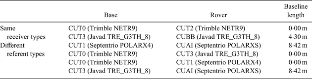
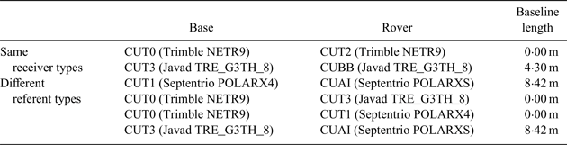
In this section, in order to assess the stability of DISBs, observation data on six zero/short baselines from the campus of Curtin University, Western Australia, on DOY (day of year) 001–003 in 2017 were used to conduct the experiment. The sampling rate of these data was 30 s, and the first two baselines used the same receiver types, while the other four used different receiver types. Table 2 shows the detailed information of these baselines. In the calculating process, for testing the variation of F-PDISBs from time to time, the intra-system double-difference ambiguities were calculated in advance with the assistance of the known baseline components, and the F-PDISBs were estimated together with the baseline components.
Receiver types and the other information on the baselines used in the experiments.
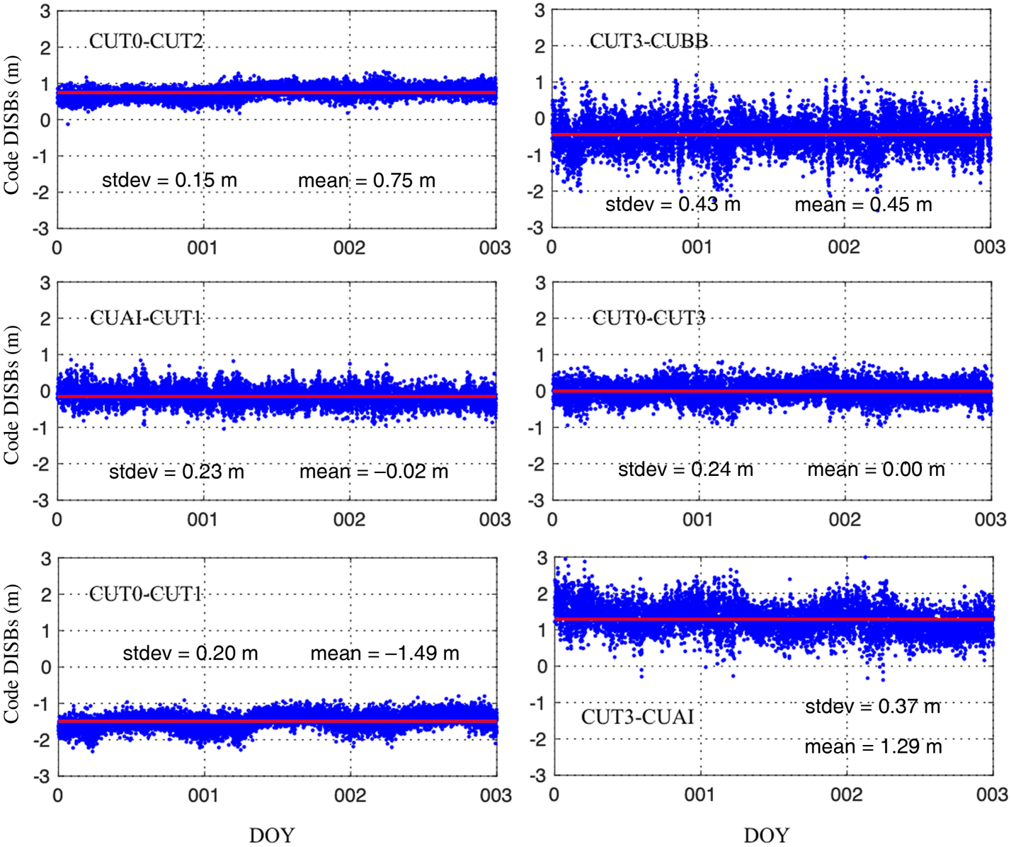
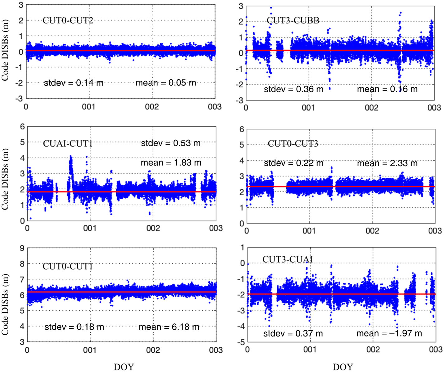
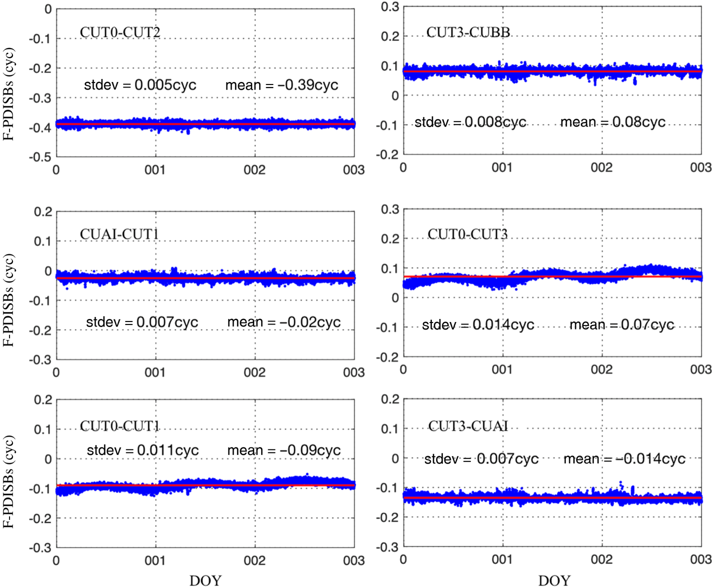
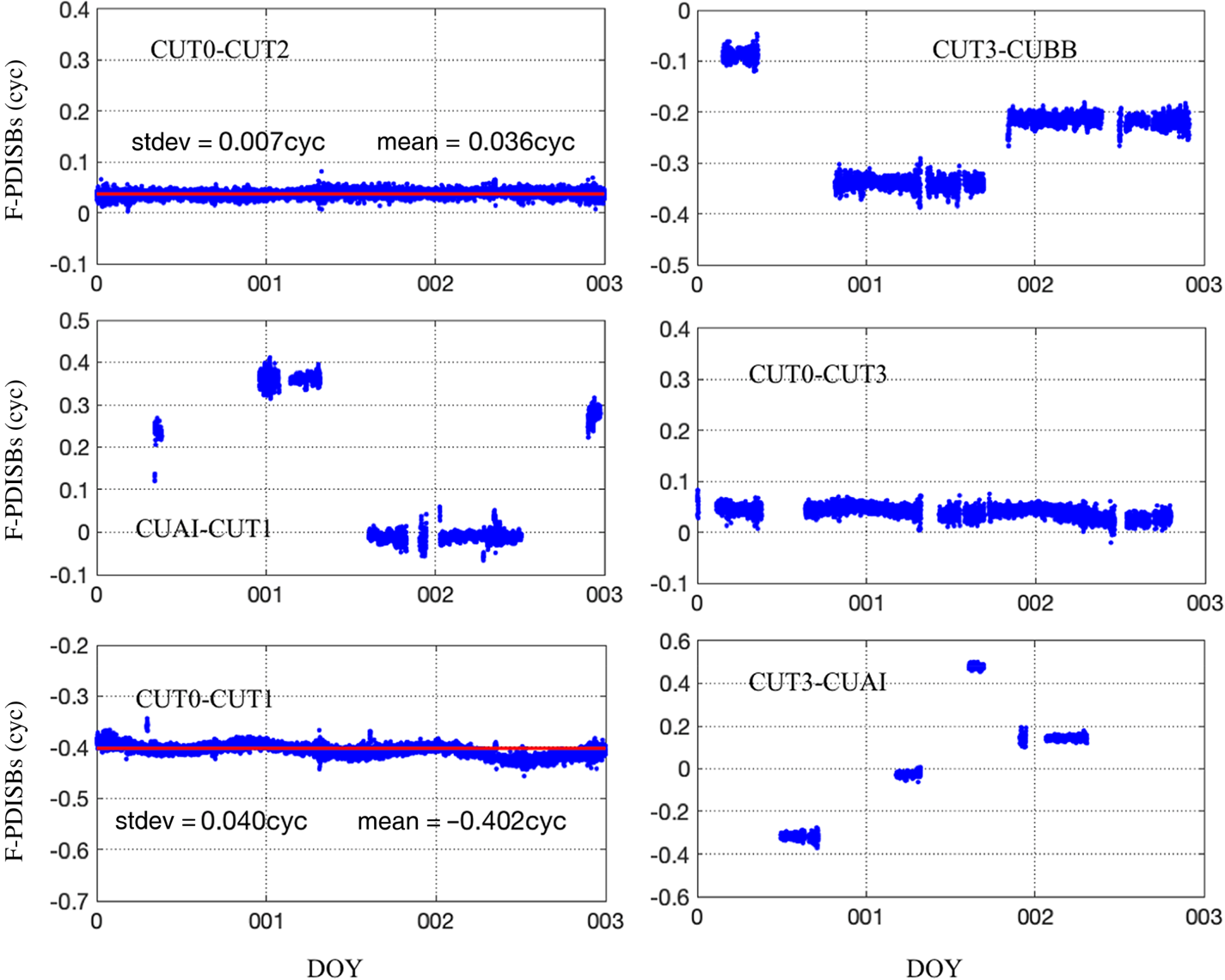
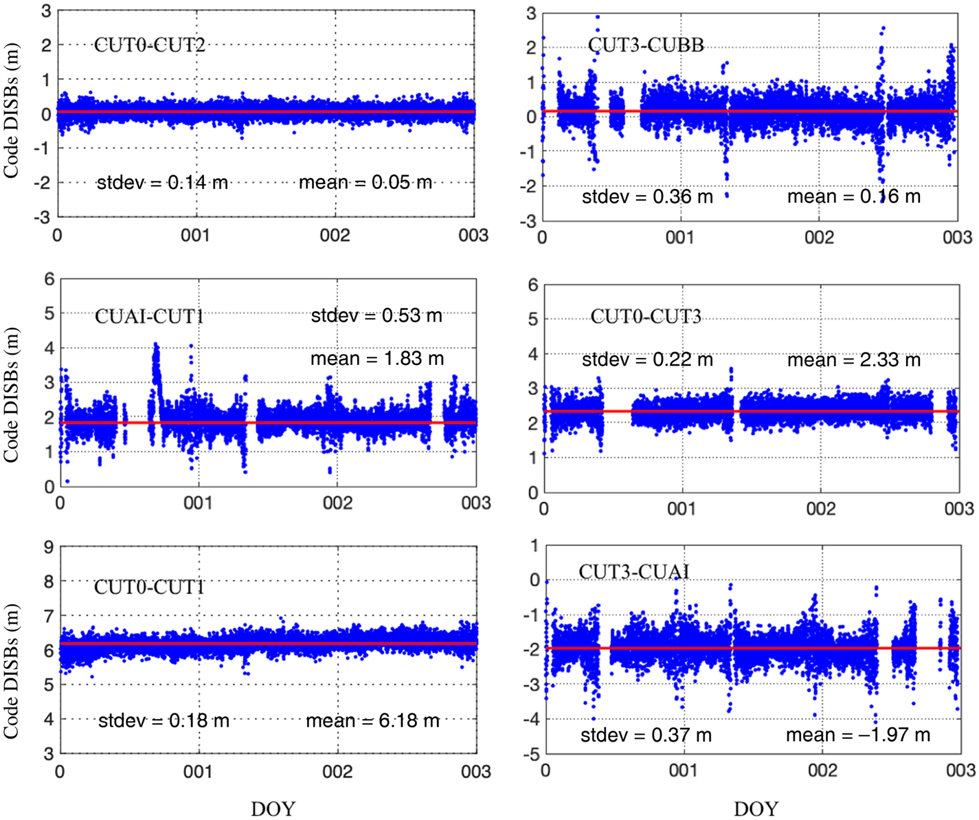
Figures 1 and 2 depict the estimated GPS L1-BDS B1 and GPS L2-Galileo E5a code DISBs for the above six baselines, respectively. Figures 3 and 4 show the GPS L1-BDS B1 and GPS L1-Galileo E5a F-PDISBs for these baselines. In these groups the three days' data are combined together to verify the stability of the code DISBs and F-PDISBs. It should be noted that the observed Galileo satellites for some receivers were less than one (for code DISBs) or two (for F-PDISBs), thus we only give the code DISBs and F-PDISBs when they can observe Galileo satellites. For GPS L1-BDS B1, from Figure 1, we can see that for the above three baselines (CUT0-CUT2, CUT3-CUBB, CUT1-CUAI), regardless of the random terms caused by observation noises, the code DISBs are very stable. However, for the bottom three baselines (CUT0-CUT3, CUT0-CUT1, CUT3-CUAI), besides the random terms, there are attenuations for the code DISBs series, even for the zero-baseline ‘CUT0-CUT1’ where no multipath effect exists. Similarly, it can be seen from Figure 3 that for the baselines CUT0-CUT2, CUT3-CUBB, CUT1-CUAI and CUT3-CUAI, the time-series for F-PDISBs is stable, while it also has obvious small variations for baselines CUT0-CUT3 and CUT0-CUT1, which is consistent with the conclusions reached by Gao et al. (Reference Gao, Gao, Pan, Meng and Xia2017a, Reference Gao, Meng, Gao, Pan and Wang2018). For GPS L1-Galileo E5a, Figures 2 and 4 show that the characteristics of code DISBs and F-PDISBs are similar to GPS L1-BDS B1. In addition, it can be seen from Figure 4 that for baselines CUT3-CUBB, CUAI-CUT1, CUT0-CUT3 and CUT3-CUAI, the F-PDISBs changed as well as the single-difference ambiguity of the first pivot satellite changed. Furthermore, in order to test the relationship between single-difference ambiguities and phase DISBs, the F-PDISBs of baseline CUT0-CUT2 for three days were calculated the results are shown in Figure 5, respectively. From Figure 5 it can clearly be seen that the F-PDISBs are different if the single-difference ambiguities are different in the initialisation time.
GPS L1-BDS B1code DISBs for the six baselines; the single-epoch DISBs are shown in blue and the average value over all epochs is shown in red.

GPS L2-Galileo E5a code DISBs for the six baselines; the single-epoch DISBs are shown in blue and the average value over all epochs is shown in red.
GPS L1-BDS B1 F-PDISBs for the six baselines; the single-epoch DISBs are shown in blue and the average value over all epochs is shown in red.

GPS L2-Galileo E5a F-PDISBs for the six baselines; the single-epoch DISBs are shown in blue and the average value over all epochs is shown in red.

GPS L1-BDS B1F-PDISBs for the baseline CUT0-CUT2 on three days; the single-epoch DISBs are shown in blue and the average value over all epochs is shown in red.

From the above experiments and analysis, we believe that, for the baselines with the same receiver types and some different receiver types (e.g., CUT1-CUAI), the code DISBs are stable and, in a given situation, the F-PDISBs are also stable. For some of the different receiver types, the code DISBs and F-PDISBs may have small variations when two frequencies are different. Thus, we can assume that if the value of F-PDISBs for the same receiver types and some different receiver types are calculated in the initialisation phase, a tightly combined inter-system model for correcting F-PDISBs in advance can be obtained.
4. PARTICLE FILTER-BASED F-PDISBs ESTIMATE METHOD
4.1. Relationship between ratio and F-PDISBs
Usually, the lambda method is employed to fix double-difference ambiguity where the performance of the fixing is normally judged by the statistical parameter ratio (Teunissen and Kleusberg Reference Teunissen, Kleusberg, Teunissen and Kleusberg1998; Teunissen, Reference Teunissen2004). The smaller the positioning residual, the larger the ratio value, and the higher ambiguity reliability can be obtained. Therefore, the closer the F-DISPBs are to the true value, the larger the ratio.
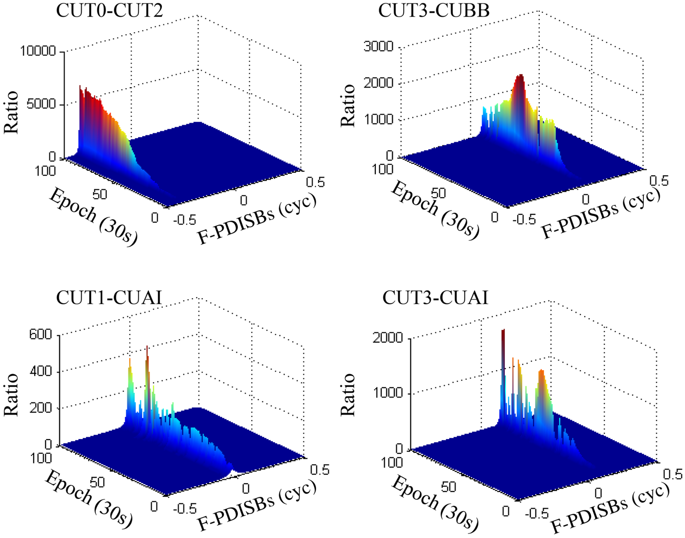
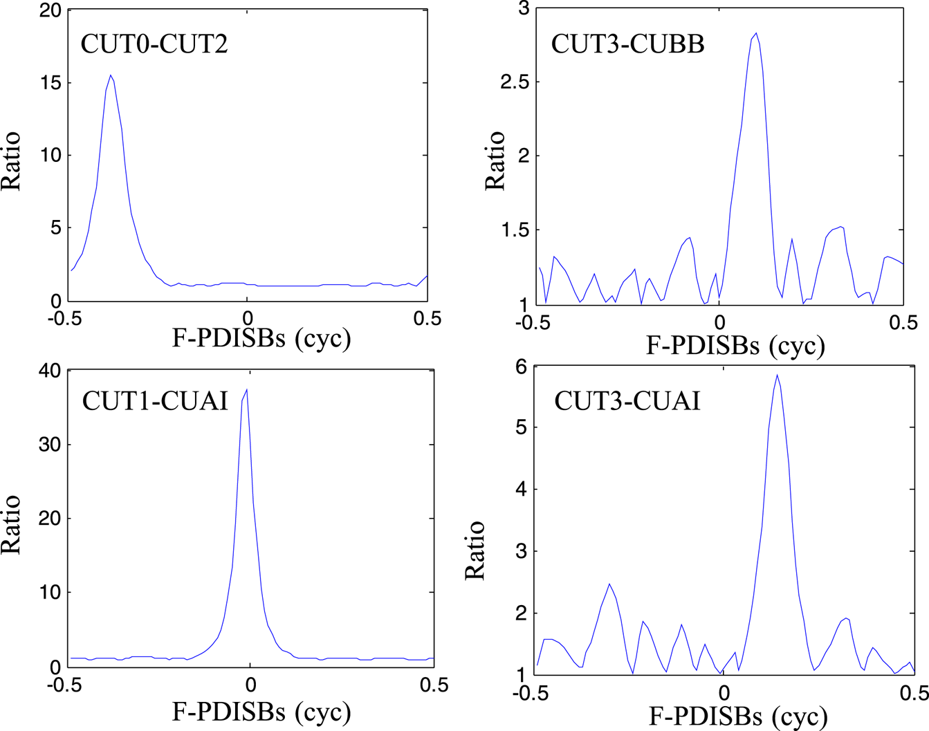
In this section, the relationship between ratio and F-DISPBs is analysed. Because they share the same characteristics, for simplicity, we only use the GPS L1-BDS B1. In order to ensure the cover range, the ranges of the F-DISPBs are limited to one wavelength, which means [−0·5, 0·5] cycles. The interval is evenly sampled with a step se of 0·01 cycles, so that there are 100 samples. Each sample value is then used as exactly known F-PDISBs to obtain the inter-system solution and we can obtain the corresponding ratio from the lambda method. The three-dimensional ratio maps of the baseline CUT0-CUT2, CUT3-CUBB, CUT1-CUAI and CUT3-CUAI for all F-PDISBs samples over the beginning 100 epochs are shown in Figure 6. The corresponding ratio results for the first epoch of these baselines are presented in Figure 7, which gives a clear image of their epoch behaviour.
Ratio results for the baseline CUT0-CUT2, CUT3-CUBB and CUT1-CUAI.

Ratio results of the first epoch for the baseline CUT0-CUT2, CUT3-CUBB and CUT1-CUAI.

Theoretically, the highest ratio value at each epoch should correspond to the true value of the F-PDISBs. Figure 6 shows the detectable peak series in a straight line with remarkably high ratio values. The peak series are almost the same F-PDISBs for all epochs and are consistent with the result in Figure 3. In general, if the F-PDISBs are given with certain accuracy, the ambiguities can usually be fixed to integer, epoch by epoch. This can also be seen from the distribution of ratio for the first epoch of the three baselines shown in Figure 7. It also can be seen from Figure 7 that although the peak of the ratio in the first epoch is not very large, it is still obvious, so we believe that it is feasible to judge the accuracy of the F-PDISBs by ratio.
4.2. Estimating F-PDISBs by particle filter
According to the above findings, it is apparent that the more accurate the F-PDISBs value is, the larger ratio value can be obtained in the process of searching for ambiguity using the lambda method. Therefore, the problem of estimation of the F-PDISBs can be attributed to the problem of finding the particle with the largest ratio value. A particle filter algorithm can select the estimated parameters from the particle set and is widely used in the processing of non-linear and non-Gaussian systems. Research by Tian et al. (Reference Tian, Ge and Neitzel2015, Reference Tian, Ge, Neitzel and Zhu2017) also shows that particle filtering has superior performance when solving inter-frequency biases (IFB) for GLONASS and inter-system biases for the same frequency systems. In addition, our research has shown that F-PDISBs for the same type of receivers and some of the baselines with different receivers are stable. Therefore, particle filtering can be introduced to solve the F-PDISBs parameters for non-overlapping frequency systems for developing the inter-system model. This paper concentrates on the sampling-importance resampling (SIR) particle filter. The solution process is as follows:
(1) In epoch k = 0, considering that only the F-PDISBs will affect the observation equations and the integer part of the PDISBs will be absorbed by ambiguity, we choose N = 100 particles as the initial value of F-PDISBs in the range of
 $[ -0{\cdot}5, \; 0{\cdot}5] $, and the weight of each particle is set as 1/100, which means $X=[ {-}0{\cdot}50, \; -0{\cdot}49\ldots0{\cdot}50] $, $W=0{\cdot}01, \; 0{\cdot}01\ldots 0{\cdot}01$], where X is the set of particles and W is the set for the weight of each particle.
(2) Consider all the particles as true values and add them to the GNSS observation equation, then we can obtain the float ambiguity and the covariance matrix corresponding to each particle.
(3) Bringing the float ambiguity and the covariance matrix into the lambda algorithm we can obtain the ratio value of each particle. When all the particle calculations are completed, calculate the sum of all the ratios and for the particle i, and the weight can be written as
(17)$$\hat {w}_k^i =\frac{\mbox{ratio}_i }{\sum_{i=1}^N {\mbox{ratio}_i}}$$(4) According to the weights calculated in the third step, using the layered resampling method, duplicate the particles with larger weights and discard the particles with smaller weights, then regenerate 100 particles and set the weight of each particle to 1/100.
(5) The F-PDISBs value and the corresponding variance calculated this time is:
(18)$$\begin{align} \hat {x}_k &\approx \sum_{i=1}^N {\hat {w}_k^i } x_k^i\end{align}$$(19)where$$\begin{align} \hat {p}_k &\approx \sum_{i=1}^N {( {x_k^i -\hat {x}_k } ) ^2\hat {w}_k^i }\end{align}$$${\mathop{x} \limits^{\frown}}_{k} $ is the estimated F-PDISBs and ${\mathop{p} \limits^{\frown}}_{k} $ is the corresponding variance.(6) Calculate the corresponding standard deviation (STD) value of the F-PDISBs, if the value is smaller than 0·001 cycle, particle filtering can be considered successful; if not, repeat Steps 2–5 to calculate the F-PDISBs again.





4.3. Convergence time for particle filter
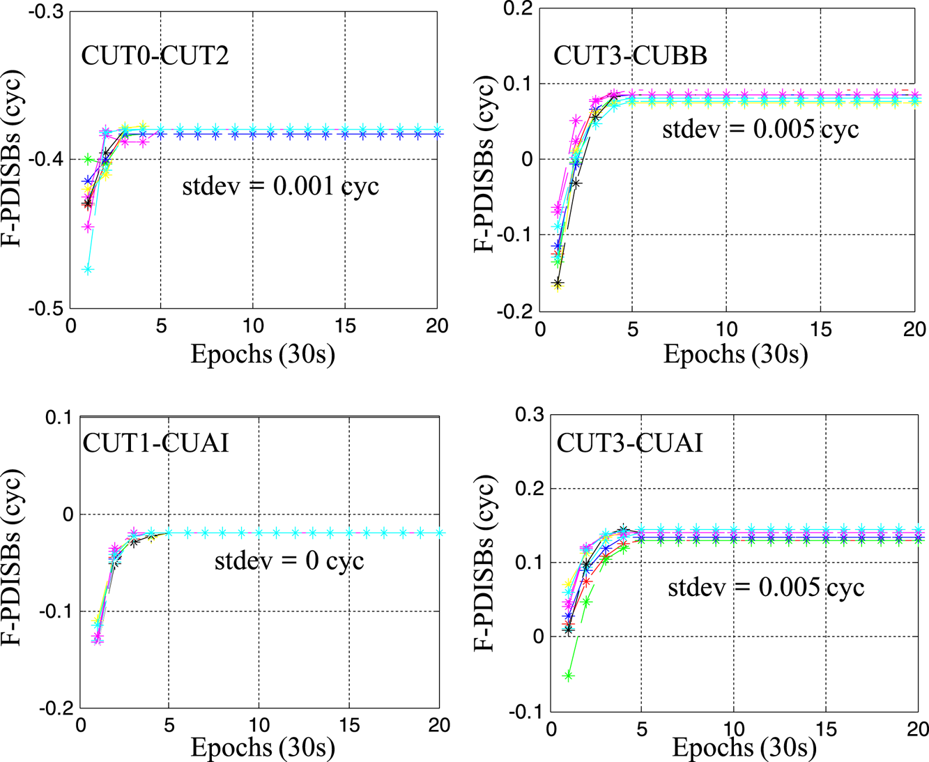
To investigate the feasibility of using particle filtering to obtain the DISBs parameters in advance, the observation data of the four baselines is examined in 10 parts; the first part starts at the first epoch and then moves forwards with a step size of one epoch. The convergence times of the 10 parts of the four baselines are shown in Figure 8. Each line shows the F-PDISBs estimates for a single part and ends at epoch 20. To show the results of each calculation more clearly, every point is marked with a star symbol. It can be seen from Figure 8 that for the four baselines, the particle filter can obtain converged F-PDISBs within five to 10 epochs. Therefore, we believe that it is feasible to use particle filter to solve the F-PDISBs parameters in several epochs for the short baseline consisting of the same receiver types and some different receiver types.
Convergence procedures of the estimated F-PDISBs versus the number of epochs.

4.4. Positioning performance of inter-system model
When the code DISBs and F-PDISBs are corrected in advance, an inter-system model is achieved. In theory, the inter-system model not only introduces at least one more redundancy, but also assures the positioning quality when very few satellites are visible for a system. Usually in complex environments such as urban canyons, buildings will block the satellites, so the visible satellites for each system are few. To simulate positioning in complex environments, experiments were conducted under two cases. In the first case, the performance of the inter-system model and intra-system model with cut-off angles from 10° to 40° was tested. Furthermore, for directly testing the positioning performance with different visible satellites, in the second case the positioning experiment was carried out with six to nine satellites, respectively, which were chosen in descending order of elevation. The observation data of baseline CUT3-CUBB on DOY 001, 2017 was used to conduct the positioning experiment; the coordinates of the two stations are precisely known from the Curtin University weekly solution and the baseline errors are the difference between the estimated baseline length and precise reference baseline.
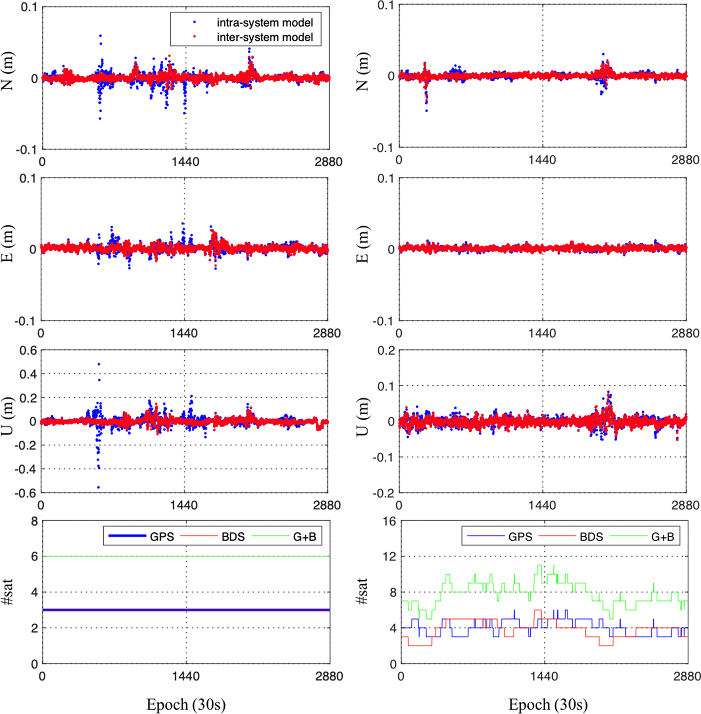
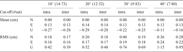
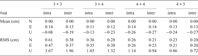
The statistics of the positioning results and the improvement of the positioning accuracy of the two cases are presented in Tables 3–5. From Tables 3 and 4 it can be observed that, due to the biases of F-PDISBs, the mean value of the intra-system model is a little smaller than the inter-system model. However, the positioning accuracy of the inter-system model is better than the intra-system model. It can be seen from Table 5 that when only six satellites are visible, the positioning accuracy improvements of the inter-system model reach up to 37·0% /21·3% / 46·6% for the East/North/Up directions, respectively. Figure 9 further shows horizontal (N, E) position scatter and the corresponding vertical (U) time-series of the baseline CUT3-CUBB under 3 + 3 visible satellites and 40° cut-off angles. It can quite clearly be seen that the time-series obtained by the inter-system model is more concentrated than the intra-system model, indicating that the positioning accuracy of the inter-system model is better. As more and more satellites are visible, the positioning performance of the two models tends to be close, but the inter-system model is always slightly better than the intra-system model.
Horizontal (N, E) position scatter and corresponding vertical (U) time-series of the baseline CUT0-CUT2 under 3 + 3 visible satellites (left) and 40° cut-off angles (right).

Mean value and Root Mean Square (RMS) of positioning results for inter-system model and intra-system model with different cut-off angles (°).
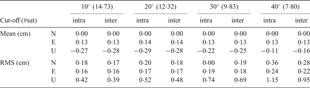
Note: #sat = mean number of satellites.
Mean value and RMS of positioning results for inter-system model and intra-system model with different visible satellites.
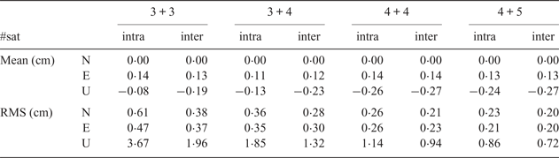
Note: #sat #equals; mean number of satellites.
Improvement of positioning accuracy from inter-system model to intra-system model.

Note: #sat #equals; mean number of satellites.
5. CONCLUSIONS
This paper proposed a particle filter-based inter-system positioning model for non-overlapping frequency CDMA systems. The stability of GPS L1-BDS B1, GPS L2-Galileo E5a phase/code DISBs, the feasibility of calculating F-PDISBs by particle filter and the positioning performance of the inter-system using six known baselines were assessed. The following conclusions are achieved:
(1) Regardless of the random terms caused by the observation noises, the phase and code DISBs for the baselines with the same receiver types and some of different receiver types are rather stable over time. Thus, we can assume that if the values of F-PDISBs for these baselines can be calculated in the initialisation phase, a tightly combined inter-system model for correcting F-PDISBs in advance can be obtained.
(2) The closer the F-PDISBs to the true values, the larger the ratio is, thus a particle filter-based F-PDISBs estimation method in which the likelihood function is built according to the ratio values is applied in this paper, and the experimental results show that it is feasible to use a particle filter to solve the F-PDISBs parameters in several epochs for the short baseline.
(3) In a complex environment the positioning accuracy of the inter-system model is better than the intra-system model. As more and more satellites are visible, the positioning performance of the two models tends to be closer, but the inter-system model is always slightly better than the intra-system model. Therefore, the inter-system model can take the place of the intra-system model to improve the positioning accuracy.
These results effectively demonstrate that our method can achieve an inter-system positioning model for non-overlapping frequency CDMA systems for the same receiver types and some of the different receiver types short baselines. When using the receiver pair, the F-PDISBs characteristic can be tested by using a short baseline first. For baselines with small variations of the F-PDISBs, it is recommended to use the method proposed by Gao et al. (Reference Gao, Meng, Gao, Pan and Wang2018), which uses the random walk process slow variation of F-PDISBs.
ACKNOWLEDGEMENTS
This work is partially supported by the Primary Research & Development Plan of Jiangsu Province (BK20171353), the National Natural Science Foundation of China (No. 41574026, No. 41774027) and the Research and Innovation Program for Graduate Students in Jiangsu Province of China (KYCX17_0149). The authors gratefully acknowledge Curtin University for providing the observation data. The authors also thank the China Scholarship Council for funding the first author to study at the University of Nottingham for one year. Miss Roxanne Parnham at the Sino-UK Geospatial Engineering Centre of the University of Nottingham is acknowledged for proofreading this paper.