1. Introduction
The forecast or projection of mortality rates has played an essential role in many areas such as demography, insurance and social policy. For instance, mortality forecasts assist demographers to perform population projections and actuaries to provide guidance on many aspects of life insurance markets and products, see Koissi & Shapiro (Reference Koissi and Shapiro2008). The accuracy and reliability of mortality forecasts is also important to consider, as there may be adverse effects on pension funds and annuity issuers if mortality forecasts are not sufficiently accurate. Overestimated mortality rates will cause a high-risk profile for pension funds and annuity insurers and underestimation will produce excess premium costs for policyholders, see Giacometti et al., (Reference Giacometti, Bertocchi, Rachev and Fabozzi2012). Consequently, actuaries and statisticians have gradually developed a range of models to more adequately model mortality rates. The most popular of these have been based on the Generalised Linear Model (GLM) regression family. In this paper, we seek to extend such models to the Generalised Linear Autoregressive Moving Average (GLARMA) family of time series regression models. We demonstrate that this is a natural extension to actuarial GLMs. The GLARMA regression model extensions can readily incorporate the time series structure of mortality projection models while importantly accommodating a new feature we have identified as being both statistically and practically beneficial and significant in understanding mortality time series structure, namely the long memory structure.
This new structure has previously been underexplored in the mortality modelling literature. In this work, we have statistical evidence of the significance of this new feature and we demonstrate how to naturally incorporate it into the GLM extension of GLARMA regression models, more widely used in time series literature. This is practically important as it can improve the forecast performance of mortality projection and it also removes identification considerations otherwise present in standard GLM formulations such as the Lee–Carter (LC) class of models.
1.1 Background on univariate mortality modelling
In the literature on single age group mortality models, either mortality rate or annual death count for a certain age group is typically modelled. When deciding upon possible models to consider for such mortality data, one may crudely consider four basic research directions that have emerged in this literature: the exploration of appropriate regression structures; the incorporation of stochastic factors; the exploration of the appropriate classes of regression distribution; and the estimation of computationally efficient and accurate techniques in both frequentist and Bayesian contexts. In this brief review, we will concentrate on aspects specifically of relevance to extensions central to this work, for more detailed descriptions and background, see references in Macdonald et al., (Reference Macdonald, Richards and Currie2018).
When population dynamic models such as those of Gompertz (Reference Gompertz1825) were calibrated to mortality data, they often failed to provide reasonable estimates of death rates across all age group stratifications, especially in older age groups 80+. Consequently, statistical regression models were developed, for instance, in Juel (Reference Juel1983) in which they proposed a model illustrating the relationship between demographic factors and age-specific mortality rates. The number of deaths for a particular age group x was found to follow a Poisson distribution and the constant mortality rate  $\mu_x$ at age x could be expressed by the function
 $\mu_x = bx^k$, where b and k are parameters to be estimated. Macdonald (Reference Macdonald1996) also confirmed that the Poisson distribution is an appropriate choice for the number of deaths with the mean being the product of total central exposure
 $E_x$ and a constant mortality rate
 $\mu_x$. Forfar et al., (Reference Forfar, McCutcheon and Wilkie1988) proposed a graduation model and studied the parameter estimation with confidence intervals and the construction of a complete mortality table based on the graduated mortality rates. Both Renshaw et al., (Reference Renshaw, Haberman and Hatzopoulos1996) and Sithole et al., (Reference Sithole, Haberman and Verrall2000) further developed graduation type models in which the log of the mortality rate was adopted as the intensity function in an overdispersed Poisson distribution. In these graduation type models, the mean function incorporating both age effects in Legendre polynomials and time trends is given by
 \begin{equation*}{\ln}(\mu_{x,t})=\beta_0+\sum_{j=1}^{s}\beta_j L^{(j)}(x)+\sum_{i=1}^{r}\alpha_i t^i \end{equation*}
where the Legendre polynomials  $L^{(n)}({\cdot})$ of degree n is generated by
 \begin{equation*}L^{(0)}(x)=1, \ \ L^{(1)}(x)=x, \ \ (n+1)L^{(n+1)}(x)=(2n+1)xL^{(n)}(x)-nL^{(n-1)}(x) \ \ \mbox{for} \ \ n\geq1 \end{equation*}
This is an extension of the conventional parametric graduation models, which incorporate unknown deterministic linear trend effects in mortality rates. Incorporating temporal regression structure to capture the trend of mortality could also be done via smoothing splines. Currie et al., (Reference Currie, Durban and Eilers2004) considered univariate and bivariate Poisson regression models, with deterministic unknown parameters in the regression. In this work, the extension was to incorporate a bivariate tensor product P-spline for the covariates age and year (Currie & Durban, Reference Currie and Durban2002). This approach using P-splines rather than B-splines introduces a penalty term for smoothness into the regression model.
Following these extensions of regression models, stochastic components were gradually incorporated into the linear predictor structures in the regressions. For instance, Brouhns et al., (Reference Brouhns, Denuit and Vermunt2002) and later Renshaw & Haberman (Reference Renshaw and Haberman2006) proposed variations of GLM with Poisson random variation for the number of deaths which incorporated a stochastic period effect  $\kappa_{t}$ on the logarithm of mortality rates. This type of structure in the mortality modelling literature is often referred to as a single age group (univariate) stochastic period effect model, which is the univariate equivalence of the famous multi-age group (multivariate) version of the widely used LC model (Lee & Carter, Reference Lee and Carter1992), applied to model mortality rates across multiple age groups simultaneously. Moreover, the period effect on the mortality rates can be modelled directly by a time series model. Other authors such as Cossette et al., (Reference Cossette, Delwarde, Denuit, Guillot and Marceau2007) and Delwarde et al., (Reference Delwarde, Denuit and Partrat2007b) used GLM structure replacing the Poisson member of the natural exponential family with the binomial or negative binomial choices to model potential over or under-dispersion, respectively, in mortality data.
The LC model is often considered as a benchmark model. However, International Monetary Fund Monetary and Capital Markets Department (2012) reported that the mortality rates estimated by LC models are consistently underestimated. Consequently, the LC model has been extended to adopt different structures and to model various responses (see Table 1 for a list of these models).
Extensions to the LC model

Note:  $ \alpha_x$ is constant for age group x,
 $ \kappa_t^{(i)} $ is the ith component period effect,
 $\beta_x^{(i)} $ is the corresponding coefficient for age group x,
 $\zeta _{t-x}$ is the cohort effect,
 $\bar{x}$ is the average age in the sample range and
 $ q_{x,t} = 1{-}\exp({-}\mu_{x,t})$ is the probability that an individual aged exactly x at exact time t will die between t and
 $t + 1 $.
Following the development of the LC model, Renshaw & Haberman (Reference Renshaw and Haberman2003) introduced a multiperiod  $\sum_{i=1}^{k}\beta_x^{(i)} \kappa_{t}^{(i)}$ extension, where
 $\beta_x^{(i)}$ represents how rapidly or slowly mortality at each age varies when the general level of mortality
 $\alpha_x$ is fixed at a certain level. Renshaw & Haberman (Reference Renshaw and Haberman2006) extended the LC model to extrapolate age-specific cohort effects
 $\zeta _{t-x}$ and age-specific period effects
 $\kappa_{t}$, and variations of this model were also explored in Currie (Reference Currie2006). Then Cairns et al., (Reference Cairns, Blake and Dowd2006) proposed a new mortality model for
 $\mbox{logit} (q_{x,t})=\ln \frac{q_{x,t}}{1-q_{x,t}}$ using two factors. The first factor models mortality at all age groups in an equal manner and the second factor models mortality being proportional to a specific age group. Further extensions were introduced by Cairns et al., (Reference Cairns, Blake, Dowd, Coughlan, Epstein, Ong and Balevich2009) and Plat (Reference Plat2009) to incorporate cohort structure and infant mortality structure.
Recently, Fung et al., (Reference Fung, Peters and Shevchenko2017) extended the LC class of models in state-space modelling frameworks to incorporate non-linear and non-Gaussian features and introduced a stochastic volatility model for the period effect in order to capture long-term mortality dynamics. Fung et al., (Reference Fung, Peters and Shevchenko2019) further improved these mortality models by incorporating cohort features under the state-space framework and these mortality models with cohort effects can be formulated, estimated and forecasted under a Bayesian state-space framework. Toczydlowska et al., (Reference Toczydlowska, Peters, Fung and Shevchenko2017) developed the family of LC stochastic mortality models by including exogenous observable demographic features that can be adopted to improve model fit and enhance forecast accuracy.
Apart from model development, parameter estimation is also an important consideration. The LC models, including many extensions, typically employed singular value decomposition (SVD) and ordinary least squares (OLS) estimation methods to extrapolate the common trend and estimate all age-specific parameters. Delwarde et al., (Reference Delwarde, Denuit and Eilers2007a) pointed out that the estimates of age-specific component  $\beta_x$ exhibit an irregular pattern in most cases, which in turn can produce irregularities in projected life tables. They proposed to resolve this issue by smoothing
 $\beta_x$ independently from other parameters. Hunt & Villegas (Reference Hunt and Villegas2015) investigated systematically convergence problems of the parameter estimates and found that the problem originated from issues with parameter identification in the LC-type models listed in Table 1. The specification of identification constraints was studied to improve the model robustness and stability. Alternatively, Czado et al., (Reference Czado, Delwarde and Denuit2005), Pedroza (Reference Pedroza2006) and Fung et al., (Reference Fung, Peters and Shevchenko2015) implemented various Bayesian approaches, incorporating appropriate choices of prior distributions to improve the robustness and convergence of parameter estimates. These approaches utilised Markov chain Monte Carlo (MCMC) methods for estimation and forecasting.
1.2 Contribution and structure
In this work, we seek to remain in the univariate class of Bayesian mortality models just discussed and we demonstrate how to naturally extend them from classical GLM regression models to the time series class of GLARMA models (Davis et al., Reference Davis, Dunsmuir and Wang1999) in which we also demonstrate the importance of long memory structure in such mortality model extensions.
Hence, a key contribution of this paper is to propose new models that combine the structure of the LC model with a generalised (Gegenbauer) autoregressive fractional integrated moving average (ARFIMA) long memory time series model structure in order to extend classical GLM frameworks to the classes of GLARMA regression models for time series of death counts. We further extend our proposed models to incorporate the graduation model to allow different mortality levels across time intervals. Moreover, we extend the Poisson distribution which has been routinely applied to model death counts to accommodate both over- and under-dispersion present in certain mortality data. This is achieved in our models via the adoption of a generalised Poisson (GP) distribution, which includes the standard Poisson distribution as a special case. We compare the performance of this flexible model and its nested sub-models in terms of accuracy of the mortality forecasts.
Our second contribution is to demonstrate the advantage of adopting a Bayesian approach via the efficient and user-friendly Rstan package in estimating our proposed models. This package utilises the efficient Hamiltonian Monte Carlo (HMC) and No-U-Turn sampler for the posterior simulation. Convergence diagnostic of posterior samples uses the number of effective samples and  $\widehat{R}$ (Gelman & Rubin, Reference Gelman and Rubin1992) to assess the sampling efficiency. The maximum likelihood (ML) method is not computationally feasible for our proposed models with unobserved variables since the resulting likelihood function involves high-dimensional integrals which are non-trivial to evaluate.
Our third contribution is to study the behaviour of mortality rates from 16 countries cross-classified by gender and age groups. To test our proposed models, we conduct simulation studies as well as real applications. Specifically, the mortality data in Australia, Iceland, UK, US and Japan are fitted into eight sub-models to evaluate the accuracy of in-sample fit and out-of-sample forecast. We believe that these five countries display a widespread of mortality features to effectively test our proposed models. Results show that forecasts from models without a long memory structure provide overestimated mortality rates which will give rise to underestimated life expectancies. This study and its findings of long memory patterns have essential applications in life table construction.
The rest of the paper is organised as follows. Section 2 reviews GLMs in the insurance area and long memory time series models for discrete data. The long memory stochastic period effect model is introduced in terms of mean function for eight sub-models and their reduced forms. Section 3 derives the Bayesian approach of our proposed models with various selection criteria. Section 4 conducts a series of simulation studies to validate the accuracy of the estimation techniques we develop for the proposed models. Section 5 presents the in-sample fitting of mortality data, out-of-sample forecast and life table construction. Section 6 concludes the paper.
2. Extending GLM Mortality Modelling with Long Memory Features
GLMs are widely adopted in actuarial science in many areas including mortality modelling. In this context, Currie (Reference Currie2013) pointed out that all of the LC-type models in Table 1 can be recast as part of the framework of GLM regressions via an appropriate choice of response distribution, link function and linear predictor form.
In general, we know that the GLM family generalises the linear regression models in two directions, namely the choices of a probability distribution for the response and the model for the mean (Ohlsson & Johansson, Reference Ohlsson and Johansson2010; De Jong & Heller, Reference De Jong and Heller2008). GLM regressions typically work with the family of natural exponential distributions, which contain a number of discrete and continuous distributions including the normal, Poisson and gamma distributions which are widely used in actuarial data analysis. Then under a GLM regression structure, one quantifies the relationship between a response variable and several explanatory variables via the following relationships on the conditional mean and variance of the regression:
 \begin{eqnarray*}\mathbb E ({\textbf{\textit{Y}}})&=&\mu=g^{-1}\left({\textbf{\textit{x}}}^{T}{\boldsymbol{\beta}}\right) , \\
\mathbb{V}\mbox{ar} ({\textbf{\textit{Y}}}) &=& \mathbb{V}\mbox{ar} (\mu)=\mathbb{V}\mbox{ar} \left(g^{-1}\left({\textbf{\textit{x}}}^{T}{\boldsymbol{\beta}}\right)\right)\end{eqnarray*}
where  ${\textbf{\textit{x}}}^{T}{\boldsymbol{\beta}}$ is the linear predictor, a linear combination of unknown parameters
 ${\boldsymbol{\beta}}$ and
 $g({\cdot})$ is the link function, which links the mean response
 $\mu$ to the linear predictor
 ${\textbf{\textit{x}}}^{T}{\boldsymbol{\beta}}$ and must be an invertible function.
One can then extend the linear predictor  $\eta_t = {\textbf{\textit{x}}}_t^{T}{\boldsymbol{\beta}}$ in such a way that the linear predictor inherits a time series structure that allows one to incorporate features such as lagged responses, as well as latent stochastic time series predictor structures for period and cohort effects. In this context, the model extensions we are particularly interested in for this paper involve generalising the types of time series model structures considered for the period and cohort effects from the classical AR(1) and random walk models typically used in mortality modelling as outlined in Table 1. We present the extensions that incorporate long memory structure for the linear predictor latent variables in the following sections.
2.1 Long memory for time series of counts
In time series literature, the modelling of time series persistence over long lags is termed long memory. There are two typical types of long memory model structure one often considers, the Fractional autoregressive integrated moving average (ARIMA) model known as the autoregressive fractionally integrated moving average (ARFIMA) model class and the more general Gegenbauer ARIMA class of models. This latter class of models simply gets its name from the fact that the representation of long memory time series structure is expressed naturally in terms of Gegenbauer polynomials as will be detailed further mathematically below. Granger & Joyeux (Reference Granger and Joyeux1980) and Hosking (Reference Hosking1981) extended the classical ARIMA model to the ARFIMA model. Hosking (Reference Hosking1981) further extended to a generalised ARFIMA model called Gegenbauer ARMA (GARMA) model, which can model data with an oscillatory damping autocorrelation function (ACF).
An important stylised fact of mortality data by age groups is the presence of a strong persistence in observed death counts. This is easily discernible by simply evaluating the sample autocorrelation structures of the time series of death counts for each age group at a national level. This feature is almost universally observed in all age groups for the majority of countries that have reporting records in the Human Mortality Database (HMD) (Shkolnikov, Reference Shkolnikov2017) and is present to differing degrees in each gender and across age groups. Based on this observation, we therefore seek to incorporate such a structure into a GLM regression model based around extensions of the LC model framework. This will involve modelling the strong autocorrelation persistence in the form of long memory time series structures. If such features are statistically meaningful in helping to more accurately explain mortality projection in-sample and for out of sample forecasting, one would expect improved model selection for such model features and more accurate forecasts. We indeed show this is the case. We will begin by explaining the GLM extension to incorporate this structure.
2.1.1 Modelling persistence via latent linear predictors in regression
In time series settings, extended temporal dependence or persistence in a time series is termed long memory. Given a stationary time series process  ${\textbf{\textit{Y}}}_{1:T} \equiv (Y_1, Y_2,\dots, Y_T)$, with
 ${\textbf{\textit{Y}}}_{1:T} \in (\mathbb{N} \cup \{0\})^T$, Beran (Reference Beran1994) defined a condition for a long memory stationary process in terms of the divergence of the ACF for
 $Y_t$ and
 $Y_{t+j}$ at lag j, such that
 \begin{equation*}\underset{n\rightarrow \infty }{\mbox{lim}}\sum_{j=-n}^{n}|\rho (j) |\rightarrow \infty \ \ \mbox{where} \ \ \rho(j)=\frac{\mbox{Cov}\left(Y_t,Y_{t+j}\right)}{\sqrt{\mathbb{V}\mbox{ar}(Y_t)\mathbb{V}\mbox{ar}\left(Y_{t+j}\right)}}\end{equation*}
The particular form of trend regression we consider involves an extension of the classical ARMA model structures typically used for period and cohort effects to accommodate long memory. This naturally brings one to consider the family of ARFIMA (p, d, q) models with mean  $\mu$ as proposed by Granger & Joyeux (Reference Granger and Joyeux1980) and Hosking (Reference Hosking1981), which describe a long memory stationary process with integrated order
 $d \in (0,1/2)$.
Definition 2.1 (ARFIMA). Consider a stationary time series process with constant  $c \in \mathbb{R}$, an ARFIMA model with order (p, d, q) is defined by
 \begin{equation*}\Phi (B)(Y_t-c )=\Theta (B)(1-B)^{-2d}\varepsilon _t, \ \ \varepsilon _t\overset{\mbox{i.i.d}}{\sim }N\left(0,\sigma _\varepsilon ^2\right)\end{equation*}
where B is the backshift operator, such that  $B Y_t=Y_{t-1}$ and
 \begin{equation}\Phi (B) = 1-\phi_{1}B- \cdots - \phi_{p}B^{p} \ \ \mbox{and} \ \ \Theta (B) = 1+\theta_{1}B+ \cdots +\theta_{q}B^{q} \end{equation}
are the autoregressive and moving average characteristic polynomials, respectively, with no common roots.
For  $d \in (0,1/2)$, the ARFIMA process is said to exhibit long memory. We note that ARFIMA model will become a short memory ARMA model for
 $d=0$ with the long memory operator
 $(1-B)^{-2d}=1$. A useful GARMA (p, d, q) model was proposed by Hosking (Reference Hosking1981) to describe data showing a slowly damping ACF with an oscillatory pattern.
Definition 2.2 (GARMA) Consider a stationary time series process with constant  $c \in \mathbb{R}$, a GARMA model with order (p, d, q) is defined by
 \begin{equation}\Phi (B)(Y_t-c )=\Theta (B)\left(1-2uB+B^2\right)^{-d}\varepsilon _t\equiv \Theta (B) \left ( \sum_{j=0 }^{\infty }\psi _{j}\varepsilon_{t-j} \right ), \ \ \varepsilon _t\overset{\mbox{i.i.d}}{\sim }N\left(0,\sigma _\varepsilon ^2\right) \end{equation}
where  $\Phi (B)$ and
 $\Theta (B)$ are defined in equation (1).
 $\psi _{j}$ denote the coefficients of the generating function for the Gegenbauer polynomials
 $(1-2uB+B^{2})^{-d}$ (Stein & Weiss 1971). These coefficients are formulated as
 \begin{equation}\psi _{j}=\sum_{q=0}^{[j/2]}\frac{({-}1)^{q}(2u)^{j-2q}\Gamma (d-q+j)}{q!(j-2q)!\Gamma (d)} \end{equation}
where  $[j/2]$ represents the integral part of
 $j/2$.
The coefficients  $\psi_j$ in equation (3) are functionally dependent on d that controls the strength of long memory and the Gegenbauer parameter u that controls the oscillation of ACF (Rainville, Reference Rainville1960). The ARFIMA model is a special case of the GARMA model when
 $u = 1$, such that the operator
 $(1-2uB+B^2)^{-d}=(1-2B+B^2)^{-d}=(1-B)^{-2d}$. For a long memory process, ACF declines at a hyperbolic rate to zero, which is a much slower rate of decay than the exponential decay of the ARMA process. The long memory strength is controlled by the value of d and the value of u determines the cycle of the long memory process. Investigating the behaviours of ACF with different values of d and u helps actuaries to understand how long memory improves forecasting performance. In particular, when
 $u=-1$ and
 $0<d<1/4$, the ACF can be written as
 \begin{equation*}\rho (j) = ({-}1)^{\,j}\frac{\Gamma (1-2d)\Gamma (j+2d)}{\Gamma (2d)\Gamma (j-2d+1)} \sim \mbox{constant}\cdot ({-}1)^{\,j} j^{4d-1} \mbox{, as} \ \ j\rightarrow \infty \nonumber\end{equation*}
For ARFIMA(0, d, 0) with  $u=1$ and
 $0<d<1/4$, it is given asymptotically by
 \begin{equation*}\rho (j) = \frac{\Gamma (1-2d)\Gamma (j+2d)}{\Gamma (2d)\Gamma (j-2d+1)} \sim \mbox{constant}\cdot j^{4d-1} \mbox{, as} \ \ j\rightarrow \infty \nonumber\end{equation*}
In addition, we note that the closed form ACF for the GARMA(0, d, 0) model with the constraint given by  $|u|<1$,
 $0<d<1/2$ is unavailable (Woodward et al., Reference Woodward, Cheng and Gray1998), but is asymptotically given by
 \begin{equation*}\rho (j) \sim \mbox{constant}\cdot j^{2d-1}{\sin}(\pi d-j\lambda _{0}) \mbox{, as} \ \ j\rightarrow \infty\end{equation*}
where  $\lambda_0=\cos^{-1}(u)$. For different values of d and u, the ACF plots of long memory time series show different patterns. Figures 1 and 2 show that the long memory strength is controlled by the value of d and the value of u determines the oscillation pattern of long memory process as displayed in the ACF.
The ACF plot for simulated data with different values of d and  $u=0.9$ for GARMA model.

The ACF plot for simulated data with different values of u and  $d=0.49$ for GARMA model.

2.2 Incorporating long memory in extended GLM mortality models
The extensions of GLM regression models, in which the linear predictor incorporates a time series structure, are often distinguished from standard GLM regression structures by the terminology generalised linear GARMA (GLGARMA) to denote that they contain a linear predictor with an Autoregressive Moving Average (ARMA) structure, see Davis et al., (Reference Davis, Dunsmuir and Wang1999). Examples of such structures in mortality modelling include latent process dynamics in the trend, such as in the LC model with a period effect. One can also think of the GLARMA models as a subclass of generalised state-space models for non-Gaussian time series, see discussions in Fung et al., (Reference Fung, Peters and Shevchenko2017).
In this paper, we are interested in the class of long memory GLMs with time series structure in the linear predictor which are denoted by the terminology GLGARMA models. The “GARMA” component refers to a type of long memory ARMA model based on Gegenbauer polynomials that act as coefficients in the GARMA model to express the persistence through a fractional difference operator.
Hence, the GLGARMA model is basically a generalised state-space model for a time series  ${\textbf{\textit{Y}}}_{1:T} \equiv (Y_1, Y_2,\dots, Y_T)$ consisting of an observation variable (death counts) and state variables (linear predictors with latent process structures for period effects and cohort effects). The canonical log link is adopted to link this function to the mean of a count distribution, to ensure the intensity is strictly positive.
In order to model discrete time series with long memory features, Yan et al., (Reference Yan, Chan and Peters2017) extended the GLM to GLGARMA model which combines the GLM and the GARMA time series model.
Definition 2.3 (GLGARMA model). Given a discrete stationary time series process and a natural  $\sigma$-algebra for the observed data filtration
 $\mathcal{F}_{1:t-1}=\sigma( Y_{1}, Y_{2},\cdots, Y_{t-1})$, a GLGARMA model with order (p, d, q) is defined by
 \begin{eqnarray*}Y_{t} |\mathcal{F}_{1:t-1} & \sim & \mbox{GP}(\mu_t, \nu), \nonumber \\\Phi (B)(\ln(\mu _{t})-c) &=& (1-2uB+B^{2})^{-d} \Theta (B)\varepsilon _t \equiv \Theta (B) \sum_{j=0 }^{\infty }\psi _{j}\varepsilon _{t-j} \nonumber\end{eqnarray*}
Sigma algebra on a set X is a collection of subsets of X that includes X itself and is closed under complement and countable unions. Data filtration is the process of choosing a subset of the data set for analysis. So natural sigma algebra  $\mathcal{F}_{1:t-1}$ for the observed data filtration means the analysis requires any subset of a given data
 $(Y_1, Y_2,\cdots , Y_{t-1})$ (
 $Y_t \in (\mathbb{N} \cup \{0\})$) including empty set. We have included this information in P.8, Definition 2.3. In this paper, the data filtration
 $\mathcal{F}_{1:t-1}$ corresponds to observed realisations of time series up to time
 $t-1$.
The GP distribution, GP $(\mu,\nu)$ has the probability mass function (pmf), mean and variance given by Definition 2.4.
Definition 2.4 (GP). A random variable Y follows a GP distribution with support on  $(\mathbb{N} \cup \{0\})$ if it has a pmf, mean and variance given by, respectively
 \begin{eqnarray*}f(y;\ \mu ,\nu )& = & \mu(1-\nu) [\mu(1-\nu) +\nu y]^{y-1}e^{-\mu(1-\nu)-\nu y}/y!,\quad \mu>0, \ -1 \leq \nu<1, \\
\mathbb{E}(Y)& = & \mu \ \ \textrm{and} \ \ {\mathbb{V}}ar(Y)=\mu(1-\nu)^{-2}\end{eqnarray*}
GP distribution is over-, under- and equi-dispersed when the dispersion parameter  $\nu \in ({-}1,1)$ is greater than, less than and equal to 0, respectively.
We develop new mortality models for death counts by combining GLGARMA model in Definition 2.3 and LC model. Let the random vector  ${\textbf{\textit{Y}}}_{x,1:T}=(Y_{x,1},Y_{x,2},\cdots,Y_{x,T})$ denote the death count series for age group
 $x \in \left\{ x_1,\cdots , x_g \right\}$ with
 $Y_{x,t} \in (\mathbb{N} \cup \{0\})$ and year
 $t \in \left\{1,\cdots , T \right\}$. The natural sigma algebra for the observed data filtration is defined as
 \begin{equation}\mathcal{F}_{x,1:t-1}=\sigma\left( Y_{x,1}, Y_{x,2},\ldots, Y_{x,t-1}\right) \end{equation}
The vector of central exposures to death risk in the middle of age interval x is  ${\textbf{\textit{E}}}_{x,1:T}= \left(E_{x,1}, E_{x,2}, \ldots, E_{x,T}\right)$.
2.2.1 Single age group long memory Lee–Carter model
The Gegenbauer long memory LC model for single age group is given by the following definition.
Definition 2.5 (Proposed model of order (p, d, q)). Condition on the central death rate  $ \mu_{x,t}(\kappa_{x,t})$ and central exposure
 $ E_{x,t}$ where
 $\kappa_{x,t}$ denotes the period effect, we assume that
 $Y_{x,t} |{\mathcal{F}_{x,1:t-1}},\break E_{x,t},\mu_{x,t}(\kappa_{x,t})$ forms a Markov process,
 \begin{eqnarray}Y_{x,t} |{\mathcal{F}_{x,1:t-1}},E_{x,t},\mu_{x,t}(\kappa_t) &\sim& {\textrm{GP}}( E_{x,t}\mu_{x,t}(\kappa_t),\nu_{x} ), \nonumber \\
\Phi_x(B){\ln \mu_{x,t}} &=& \mathbb{B}_x(t;\ r,l, {\boldsymbol{\tau}})+\kappa_{x,t}+ (1-2u_xB+B^{2})^{-d_x} \Theta_x (B)( \varepsilon _{x,t}),\\
\kappa_{x,t} & =& \eta_x \kappa_{x,t-1} +\varepsilon_{x,t}^{\kappa}, \nonumber \\
\mathbb{B}_x(t;\ r,l, {\boldsymbol{\tau}}) & = & \sum_{i=1}^{l} \left ( a_{x,i}^{(0)}+a_{x,i}^{(1)}(t-\tau_i)\right.\nonumber\\
&& \qquad + \left. a_{x,i}^{(2)}(t-\tau_i)^2+a_{x,i}^{(3)}(t-\tau_i)^3 +\cdots a_{x,i}^{(r)}(t-\tau_i)^r \right )\cdot \mathbf{1}_{t \in [\tau_{i},\tau_{i+1}]} \nonumber \end{eqnarray}
where  $0<d_x<1/2$,
 $|u_x|<1$,
 $\Phi_x(B)$ and
 $\Theta_x(B)$ are defined in equation (1) with age-specific coefficients for each age group x. The error terms are defined as
 $\varepsilon _{x,t} \overset{\mbox{i.i.d}}{\sim } {N}(0,\sigma_{x,\varepsilon}^2)$ and
 $\varepsilon_{x,t}^{\kappa} \overset{\mbox{i.i.d}}{\sim } {N}(0,\sigma_{x,\varepsilon^{\kappa}}^2\!)$. In order to present a graduation (time) effect, the constant c is replaced by the B-spline
 $\mathbb{B}_x(t;\ r,l, {\boldsymbol{\tau}})$. This temporal spline is of order r with l knot points
 ${\boldsymbol{\tau}}=(\tau_1,\ldots,\tau_l)$ and it can be reduced to an intercept
 $\alpha_x$ as a special case. Furthermore, the period effect
 $\kappa_{x,t}$ for each age group is a latent AR(1) process in which we enforce stationarity through
 $|\eta_x|<1$.
Remark 2.1. We remark that higher order variants of the latent intensity such as AR(p) models for the period effect can easily be accommodated. In practice, we find it suitable to focus our attention here on the classical LC-type model which has an AR(1) structure, except we extend the classical LC model by restricting ourselves to strictly second-order stationary processes.
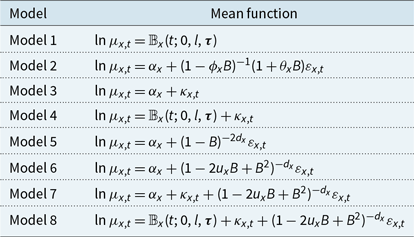
Considering some special cases of equation (5), the long memory LC model can be further divided into eight different sub-models with their mean functions defined in Table 2. In Appendix A, we consider these eight sub-models and perform simulation studies to assess the accuracy of the parameter estimates for these models.
Eight different sub-models where models 1,4,8 are graduation models, models 3,4,7,8 are LC-type models, models 1–4 are short memory models and models 5–8 are long memory models

2.3 Relationship between LC period effect models and long memory extensions
In this section, we explain the connection between LC model with a non-stationary period effect and the long memory model. There are several disturbance terms in our proposed models, which come from the latent state period effect  $\kappa_{x,t}$ specification. These disturbance terms in a linear univariate structural time series model can be combined in an appropriate manner to obtain a reduced form canonical time series, accommodating the fractional difference operator that produces the persistence in the long memory component of the model (Harvey, Reference Harvey1990). For instance, Hyndman et al., (Reference Hyndman, Koehler, Ord and Snyder2008) showed that an ARIMA form is obtained by eliminating the state variables from a linear innovation state-space model. Such a reduced form when available can be beneficial for interpreting aspects of the state-space model such as the ACF and the autocovariance function, which in some cases may be obtained in closed form.
To see why this is possible, we note that such a form can be easily represented by Wold representation (Wold, Reference Wold1938) and hence variance, autocorrelation structure and the latent process can be obtained. The Wold theorem plays a central role in time series analysis, and it indicates that the dynamic of any purely non-deterministic covariance-stationary process can be arbitrarily well approximated by an ARMA process. This simplified form helps us to understand better the impact of long memory features on the period effect. We study the reduced form of the mean function in model 7 as an example since other models are just special cases. Model 7 has the following structure:
 \begin{eqnarray}\Phi_x(B){\ln \mu_{x,t}} & = & \alpha_x+\kappa_{x,t}+ (1-2u_xB+B^{2})^{-d_x} \Theta_x (B) \varepsilon _{x,t},\\
\kappa_{x,t} & = & \eta_x \kappa_{x,t-1} +\varepsilon_{x,t}^{\kappa} \nonumber \end{eqnarray}
We have
 \begin{align}\kappa_{x,t}-\eta_x \kappa_{x,t-1} & = (1- \eta_x B)\kappa_{x,t} = \varepsilon_{x,t}^{\kappa} \Rightarrow \kappa_{x,t} = \frac{\varepsilon_{x,t}^{\kappa}}{(1- \eta_x B)},\nonumber\\[4pt]
\kappa_{x,t} -\kappa_{x,t-1} & = \frac{(1-B)}{(1- \eta_x B)}\varepsilon_{x,t}^{\kappa}\end{align}
By taking differences of equation (6) with respect to time t and  $t-1$, we obtain
 \begin{equation*}\Phi_x(B)(\ln \mu_{x,t}-\ln \mu_{x,t-1}) = (\kappa_{x,t}- \kappa_{x,t-1})+ (1-2u_xB+B^{2})^{-d_x} \Theta_x (B)( \varepsilon _{x,t}- \varepsilon _{x,t-1}) \nonumber \\\end{equation*}
By substituting equation (7) and eliminating  $(1-B)$, we obtain the following reduced form:
 \begin{eqnarray}\Phi_x(B)\ln \mu_{x,t} & = & \frac{1}{(1- \eta_x B)} \varepsilon_{x,t}^{\kappa}+ (1-2u_xB+B^{2})^{-d_x} \Theta_x (B) \varepsilon _{x,t} \nonumber\end{eqnarray}
For the case that  $\varepsilon_{x,t}^{\kappa}$ and
 $\varepsilon _{x,t}$ are both i.i.d white noise, we have a transformed GARMA model represented as
 \begin{eqnarray}\Phi_x(B)\ln \mu_{x,t} & = & \left [ \frac{1}{(1- \eta_x B)}+ (1-2u_xB+B^{2})^{-d_x} \Theta_x (B) \right ] \varepsilon _{x,t} \nonumber\end{eqnarray}
Based on the generating function  $\displaystyle \frac{1}{(1-cx)}=\sum_{i=0}^{\infty}(cx)^i$ for constant c and equation (2), we have
 \begin{equation*}\frac{1}{(1- \eta_x B)} = \sum_{i=0}^{\infty}(\eta_x^i)B^i \ \ \mbox{and} \ \ (1-2u_xB+B^{2})^{-d_x} = \sum_{i=0 }^{\infty }\psi_{x,i}B^i\nonumber\end{equation*}
For a transformed GARMA (0, d, 0) model, we have
 \begin{eqnarray}\ln \mu_{x,t} & = & \sum_{i=0 }^{\infty }(\eta_x^i+\psi_{x,i}) \varepsilon _{x,t-i} \end{eqnarray}
Figure 3 shows the impact of the period effect on the ACF and spectral density function of GARMA model. The spectral density represents an autocovariance function in the frequency domain, which is obtained via Fourier transform. This frequency domain approach involves projection of the signal onto a sinusoidal basis and is then able to capture and describe the oscillatory features of data in an interpretable manner. For the GARMA model, the peak indicates that a substantial source of variability is contributed by this frequency band around the peaks. Furthermore, the value of u can be easily determined by the location of the peak. For the transformed GARMA model in equation (8), the strength of the long memory is reduced and the spectral density plots show that the long memory pattern becomes less symmetric around the dominant frequency.
The ACF plot and spectral density plot for GARMA model with  $d_x=0.45$ and
 $u_x=0.9$ and transformed GARMA model with
 $d_x=0.45$,
 $u_x=0.9$ and
 $\eta_x=0.9$.

3. Bayesian Estimation of Long Memory Mortality Regression Models
The Bayesian approach is widely applied in mortality models because it can provide several advantages. First, prior beliefs can be incorporated into model structures. Several studies have been performed on the prior specification in mortality modelling and demographic research, for instance, in Girosi & King (Reference Girosi and King2008), they improved existing Bayesian models by showing how to correctly incorporate prior knowledge for explanatory variables. They also proposed guidelines for choosing suitable priors in the presence of partial prior ignorance. Fung et al., (Reference Fung, Peters and Shevchenko2015) provided some general assumptions for the priors of the LC model under the Bayesian approach. Furthermore, they suggested a new form of identification constraint for estimating the model under the state-space framework for Bayesian demographic models. Fung et al., (Reference Fung, Peters and Shevchenko2019) and Fung et al., (Reference Fung, Peters and Shevchenko2017) further developed a cohort-based state-space model formulation. A Bayesian approach is then developed to provide the quantification of parameter uncertainty for mortality forecasts. Second, the Bayesian approach replaces the computation complexities in evaluating the marginal likelihood function, which involves high-dimensional integration of latent variables in the ML approach, by posterior sampling. Third, posterior predictive distributions provide distributional forecast summaries such as Bayesian prediction intervals. These intervals incorporate more sources of variability than the confidence intervals under the classical frequentist approach and are, therefore, often preferred.
3.1 Posterior predictive distribution
One clear advantage of a Bayesian approach is that it replaces the high-dimensional integrals in evaluating the marginal likelihood functions in the ML approach with posterior sampling. This advantage particularly applies to our proposed model because the model involves latent variables in both mean  $\mu_{x,t}$ and period effect
 $\kappa_{x,t}$ functions. In this section, we introduce the Bayesian approach to estimate the proposed model in Definition 2.5. The basic idea of the Bayesian approach can be described by the following definition and equations.
Definition 3.1 (Posterior distribution). Consider a set of observed values  ${\textbf{\textit{y}}}_{x,1:T} = (y_{x,1},\break y_{x,2}, \ldots, y_{x,T})$ with each
 $y_{x,t} \in (\mathbb{N} \cup \{0\})$, central exposure
 ${\textbf{\textit{E}}}_{x,1:T}$ and the vector of unknown parameters
 \begin{equation*}{\boldsymbol{\vartheta}}_x =\left(\alpha_x, a_{x,i}^{(0)}, \cdots, a_{x,i}^{(r)}, \eta_x, \sigma^2_{x,\varepsilon}, \sigma^2_{x,\varepsilon^{\kappa}}, d_x, u_x,\nu_x \right)\end{equation*}
and denote the state parameters  ${\textbf{\textit{z}}}_{x,t}=[\mu_{x,t}(\kappa_{x,t}), \kappa_{x,t}]$ and
 ${\textbf{\textit{z}}}_x =[ {\textbf{\textit{z}}}_{x,1},\cdots, {\textbf{\textit{z}}}_{x,T}]$ and
 \begin{equation*}{\boldsymbol{\vartheta}}_{x}^*=[{\boldsymbol{\vartheta}}_x, {\textbf{\textit{z}}}_x]\end{equation*}
the posterior distribution for  $\boldsymbol{\vartheta}_x^*$ conditional on
 ${\textbf{\textit{y}}}_{x,1:T} $ is given by
 \begin{equation*}\pi\!\left(\boldsymbol{\vartheta}_x^* | \mathcal{F}_{x,1:T} \right)=\frac{f\!\left({\textbf{\textit{y}}}_{x,1:T} | {\textbf{\textit{E}}}_{x,1:T},\boldsymbol{\vartheta}_x^*\right)\ \pi\!\left(\boldsymbol{\vartheta}_x^*\right)}{\int f\!\left({\textbf{\textit{y}}}_{x,1:T} | {\textbf{\textit{E}}}_{x,1:T},\boldsymbol{\vartheta}_x^*\right)\ \pi\!\left({\boldsymbol{\vartheta}}_x^*\right) \ d\boldsymbol{\vartheta}_x^*}\propto f\!\left({\textbf{\textit{y}}}_{x,1:T}| {\textbf{\textit{E}}}_{x,1:T},\boldsymbol{\vartheta}_x^*\right)\pi\!\left(\boldsymbol{\vartheta}_x^*\right)\end{equation*}
where the prior densities  $\pi(\boldsymbol{\vartheta}_x)$ can be chosen based on available information or past data.
Even if there is no prior information, non-informative or reference priors can be also applied. Furthermore, the credible intervals for all parameters of interest can be constructed from posterior distributions. A credible interval is the Bayesian equivalent of the confidence interval in frequentist statistics. Credible intervals capture our current uncertainty in the location of the parameter values and thus can be interpreted as a probabilistic statement about the parameter. In contrast, confidence intervals capture the uncertainty about the interval we have obtained (i.e. whether it contains the true value or not). Thus, they cannot be interpreted as a probabilistic statement about the true parameter values. The credible interval is defined in the domain of a posterior probability distribution or a predictive distribution. Under the model structure in equation (5), the complete likelihood function for model 8, as an example, is
 \begin{eqnarray*} f\!\left({\textbf{\textit{y}}}_{x,1:T}| {\textbf{\textit{E}}}_{x,1:T}, \boldsymbol{\vartheta}_x^*\right)& = & \prod_{t=1}^{T}f\!\left(y_{x,t} | E_{x,t},{\boldsymbol{\vartheta}}_x,\mu_{x,t}\left(\kappa_{x,t}\right)\right)f\!\left(\mu_{x,t}|{\boldsymbol{\vartheta}}_x,\kappa_{x,t}\right)f\!\left(\kappa_{x,t}|{\boldsymbol{\vartheta}}_x\right) \\[3pt]
& =& \prod_{t=1}^{T}\frac{E_{x,t}\exp\!\left( \mathbb{B}_x\left(t;\ 0,l,{\boldsymbol{\tau}}\right)+\kappa_{x,t}+ \left(1-2u_xB+B^{2}\right)^{-d_x} \varepsilon _{x,t}\right)\left(1-\nu_x\right) }{\Gamma\! \left(y_{x,t}+1\right)\exp\! \left(y_{x,t}\nu_x\right) } \\[3pt]
& \times& \frac{\left[E_{x,t}{\exp}\!\left( \mathbb{B}_x\left(t;\ 0,l,{\boldsymbol{\tau}}\!\right){+}\kappa_{x,t}{+} \left(1{-}2u_xB+B^{2}\right)^{-d_x}\! \varepsilon _{x,t}\right)\!\left(1{-}\nu_x\right) +y_{x,t}\nu_x\right]^{y_{x,t}-1}}{\exp\! \left\{E_{x,t}\exp\!\left[ \mathbb{B}_x\left(t;\ 0,l,{\boldsymbol{\tau}}\right)+\kappa_{x,t}+ \left(1-2u_xB+B^{2}\right)^{-d_x} \varepsilon _{x,t}\right]\left(1-\nu_x\right) \right\}} \\[3pt]
& \times& \frac{1}{\sqrt{2 \pi}\sigma^2_{x,\varepsilon}}\exp\!\left ( \frac{\varepsilon _{x,t}^{2}}{2\sigma^2_{x,\varepsilon}} \right )\frac{1}{\sqrt{2 \pi}\sigma^2_{x,\varepsilon^{\kappa}}}\exp\!\left ( \frac{\left( \kappa_{x,t}-\eta_x\kappa_{x,t-1} \right)^{2}}{2\sigma^2_{x,\varepsilon^{\kappa}}} \right )\end{eqnarray*}
where  ${\boldsymbol{\mu}}_{x,1:t}({\boldsymbol{\kappa}}_{x,1:t})=(\mu_{x,1}(\kappa_{x,1}), \mu_{x,2}(\kappa_{x,2}), \cdots, \mu_{x,t}(\kappa_{x,t}))$. The following priors
 $\pi(\boldsymbol{\vartheta}_x)$ are adopted in this paper:
 \begin{eqnarray*} \nu_x \sim {\textrm{U}}({-}1,1), u_x\sim {\textrm{U}}({-}1,1), d_x\sim {\textrm{U}}(0,1/2), \alpha_x, a_{x,i}^{(0)}, \cdots, a_{x,i}^{(r)} \sim {\textrm{N}}({-}5,1), \\ \eta_x \sim {\textrm{U}}({-}1,1), \sigma^2_{x,\varepsilon} \sim \mbox{Gamma}(1,1)\ \mbox{and}\ \sigma^2_{x,\varepsilon^{\kappa}} \sim \mbox{Gamma}(1,1)\end{eqnarray*}
where U $(a_{\theta},b_{\theta})$ denotes the uniform priors on the range
 $(a_{\theta}, b_{\theta})$ for parameter
 $\theta$, which represents the shape parameter
 $\nu_x$, the oscillatory parameter
 $u_x$, the long memory parameter
 $d_x$ and the AR parameter
 $\eta_x$ in period effect because these parameters are uninformative and the interval for these uniform priors are the bounds for these parameters. In time series and regression settings, it is fairly common to use a normal distribution for coefficients. The model coefficients
 $\alpha_x, a_{x,i}^{(0)}, \cdots, a_{x,i}^{(r)}$ follow a normal distribution with mean equal to
 $-5$ and variance equal to 1. The setting for the mean was informed by the empirical study of the log intersect of real-life mortality data sets. Moreover, the variance setting of 1 allows for great flexibility with regard to this mean specification and makes the prior relatively uninformative when viewed on the log scale. Gamma(a, b) denoting the gamma prior with shape and scale parameters a and b is an adequate choice for positive variances
 $\sigma^2_{x,\varepsilon}$ and
 $\sigma^2_{x,\varepsilon^{\kappa}}$ (Gelman, Reference Gelman2006). To implement the proposed models efficiently, we choose the Bayesian R package Rstan, which utilises the stan program within R developed in the C++ language. The HMC sampler (Duane et al., Reference Duane, Kennedy, Pendleton and Roweth1987; Neal, Reference Neal1994) as a class of MCMC sampling methods (Metropolis et al., Reference Metropolis, Rosenbluth, Rosenbluth, Teller and Teller1953) is adopted in Rstan. For some complicated models with many parameters, the HMC sampler converges faster than the conventional samplers such as random-walk Metropolis (Metropolis et al., Reference Metropolis, Rosenbluth, Rosenbluth, Teller and Teller1953) and Gibbs sampler (Geman & Geman, Reference Geman and Geman1984). In order to closely monitor the dependence, precision and convergence of posterior samples, three measures are reported in Rstan. The first measure is the number of effective samples which indicates the effective posterior sample size after allowing for the dependence within a Monte Carlo sample. The second measure is the Monte Carlo standard error (MCSE)
 \begin{equation*}\mbox{MCSE}=\frac{\mbox{posterior standard deviation}}{\sqrt {\mbox{number of effective samples}}}\end{equation*}
which reports the error of estimation for the posterior mean. To monitor the convergence for  $k > 2$ chains of length 2n each, Gelman & Rubin (Reference Gelman and Rubin1992) proposed
 $\widehat{R}$. If
 $\widehat{R}$ is close to 1, the parameter
 ${\boldsymbol{\vartheta}}_x$ has converged.
Bayesian forecasting is another application of Bayesian inference. The predictive distribution can be derived from the Bayesian filtering equations  $f(y_{x,t}|E_{x,t},\mathcal{F}_{x,1:t-1})$, which compute the marginal posterior distribution or filtering distribution of the state
 $y_{x,t}$ at each time
 $t-1$ given the history of the measurements up to the time t. The Bayesian filter for computing the predicted distribution at the time T is given by the following Bayesian filtering equation (9). Suppose we want m-step forecasts
 ${\textbf{\textit{y}}}_{x,T+1:T+m}$ with the observed data filtration
 $\mathcal{F}_{x,1:T}$ for age group x defined in equation (4) and observed exposures
 ${\textbf{\textit{E}}}_{x,1:T+m}$. We note that
 ${\textbf{\textit{E}}}_{x,T+1:T+m}$ can not be directly observed in general. However, there are many methods to estimate
 ${\textbf{\textit{E}}}_{x,T+1:T+m}$. For example, the rational expectation model defined as a piecewise constant extension
 $E_{x,T+s}=\mathbb{E}({\textbf{\textit{E}}}_{x,1:T+s-1})$ for
 $s=1,2,\cdots,m$ can be applied to estimate future exposures
 ${\textbf{\textit{E}}}_{x,T+1:T+m}$. Alternatively, we can assume a stochastic model
 $f({\textbf{\textit{E}}}_{x,T+1:T+m}|{\textbf{\textit{E}}}_{x,1:T},{\boldsymbol{\vartheta}}_x,\mathcal{F}_{x,1:T})$ for future exposures. The posterior predictive distribution for
 ${\textbf{\textit{y}}}_{x,T+1:T+m}$ is defined as
 \begin{eqnarray}& & f({\textbf{\textit{y}}}_{x,T+1:T+m}|{\textbf{\textit{E}}}_{x,1:T+m},\mathcal{F}_{x,1:T}) \nonumber \\[3pt]
&=& \int \! {\dots}\! \int \prod_{s=1}^{m} \left[f( y_{x,T+s}|{\textbf{\textit{E}}}_{x,1:T+s},{\boldsymbol{\mu}}_{x,1:T+s}({\boldsymbol{\kappa}}_{x,1:T+s}), {\boldsymbol{\vartheta}}_x, \mathcal{F}_{x,1:T})\right.\nonumber\\[3pt]
&&\times\ f( \mu_{x,T+s}( \kappa_{x,T+s})|\mu_{x,T+s-1}( \kappa_{x,T+s-1}), {\boldsymbol{\vartheta}}_x, \mathcal{F}_{x,1:T}) \nonumber \\[3pt]
& &\left. \times\ f( \kappa_{x,T+s}| \kappa_{x,T+s-1}, {\boldsymbol{\vartheta}}_x , \mathcal{F}_{x,1:T})\right] f({\boldsymbol{\mu}}_{x,1:T}({\boldsymbol{\kappa}}_{x,1:T})| {\boldsymbol{\vartheta}}_x , \mathcal{F}_{x,1:T}) f({\boldsymbol{\kappa}}_{x,1:T}| {\boldsymbol{\vartheta}}_x , \mathcal{F}_{x,1:T}) \nonumber \\[3pt]
& &\times\ \pi({\boldsymbol{\vartheta}}_x|\mathcal{F}_{x,1:T}) d {\boldsymbol{\mu}}_{x,1:T+s}({\boldsymbol{\kappa}}_{x,1:T+s})d {\boldsymbol{\kappa}}_{x,1:T+s}d{\boldsymbol{\vartheta}}_x \end{eqnarray}
and this integral can be approximated by the Monte Carlo estimator, constructed from posterior samples according to
 \begin{eqnarray}& & \hat{f}\left( y_{x,T+s}|{\textbf{\textit{E}}}_{x,1:T+s},\mathcal{F}_{x,1:T}\right) = \frac{1}{L}\sum_{l=1}^{L}f\left(y_{x,T+s}|{\textbf{\textit{E}}}_{x,1:T+s},{\boldsymbol{\mu}}_{x,1:T+s}^{(l)}\left({\boldsymbol{\kappa}}_{x,1:T+s}^{(l)}\right), {\boldsymbol{\vartheta}}_{x}^{(l)},\mathcal{F}_{x,1:T}\right) \end{eqnarray}
where L is the number of iterations after burn-in in each MCMC sampler run given the current window of information and  ${\boldsymbol{\mu}}_{x,1:T+s}^{(l)}({\boldsymbol{\kappa}}_{x,1:T+s}^{(l)})$,
 ${\boldsymbol{\kappa}}_{x,1:T+s}^{(l)}$ and
 ${\boldsymbol{\vartheta}}^{(l)}_{x}$ are the lth draw in the posterior sample of
 ${\boldsymbol{\mu}}_{x,1:T+s}({\boldsymbol{\kappa}}_{x,1:T+s})$,
 ${\boldsymbol{\kappa}}_{x,1:T+s}$ and
 ${\boldsymbol{\vartheta}}_x$, respectively.
3.2 Model selection and forecast performance
The performance of each model is evaluated through a popular Bayesian model selection criteria called Deviance Information Criterion (DIC) (Spiegelhalter et al., Reference Spiegelhalter, Best, Carlin and Van Der Linde2014). As a generalisation of Akaike’s Information Criterion (AIC), DIC can deal with models containing informative priors, such as hierarchical models. As the priors can effectively restrict the freedom of model parameters, the number of parameters as required in the calculation of AIC is generally unclear. DIC overcomes such problems by providing an estimate for the effective number of parameters. The DIC can be calculated using the following equation:
 \begin{equation*}\text{DIC}=\bar{D}+p_D=2\bar{D}-D(\bar{{\boldsymbol{\vartheta}}}_x) \end{equation*}
where the deviance is defined as  $D(\boldsymbol{\vartheta_x} )=-2\ln(f({\textbf{\textit{y}}}_x|{\boldsymbol{\vartheta}}_x))$,
 $\bar{D}=\mathbb E_{\vartheta_x|y_x}[{-}2\ln(f({\textbf{\textit{y}}}_x|{\boldsymbol{\vartheta}}_x))]$ measures the model fit and the estimated number of parameters
 $p_{D}=\bar{D}-D(\bar{\boldsymbol{\vartheta}}_x)$ measures model complexity (Spiegelhalter et al., Reference Spiegelhalter, Best, Carlin and Van Der Linde2002).
Consider the m-step ahead forecasts  $\hat{y}_{x,t}$ given by the posterior mean or median and the observations
 $y_{x,t}$ with T time point and g age groups, the forecast performance can be evaluated by adopting three types of measures, namely residuals
 $r_{x,t}=y_{x,t}-\hat{y}_{x,t}$, percentage errors
 $p_{x,t}=\frac{r_{x,t}}{y_{x,t}}\times 100$ and scaled errors
 $\epsilon_{x,t}$ defined in equation (13). Based on
 $r_{x,t}$ and
 $p_{x,t}$, three popular criteria, namely mean absolute error (MAE), root mean squared error (RMSE) and mean absolute percentage error (MAPE), are defined, respectively, below
 \begin{align}\mbox{MAE} & =\frac{1}{g}\sum_{x=1}^{g}\left[\frac{1}{m}\sum_{t=1}^{m}|r_{x,T+t}|\right], \mbox{RMSE}=\sqrt{\frac{1}{g}\sum_{x=1}^{g}\left[\frac{1}{m}\sum_{t=1}^{m}r_{x,T+t}^2\right]} \nonumber \\[5pt]
\mbox{and}\quad \mbox{MAPE} & =\frac{1}{g}\sum_{x=1}^{g}\left[\frac{1}{m}\sum_{t=1}^{m}|p_{x,T+t}|\right] \end{align}
However  $r_{x,t}$ are scale-dependent making comparison difficult. Although
 $p_{x,t}$ are scale-free, they are sensitive to observations close to zero. Hence, the fourth criterion we adopt is mean absolute scaled error (MASE), which is defined as
 \begin{equation}\mbox{MASE}=\frac{1}{g}\sum_{x=1}^{g}\left[\frac{1}{m}\sum_{t=1}^{m}|\epsilon_{x,T+t}|\right] \end{equation}
making use of the scaled errors
 \begin{equation}\epsilon_{x,T+t}=\frac{r_{x,T+t}}{\frac{1}{m-1}\sum\limits_{t=2}^{m}|y_{x,T+t}-y_{x,T+t-1}|} \end{equation}
proposed by Hyndman & Koehler (Reference Hyndman and Koehler2006). Furthermore, similar approach can also be applied to evaluate estimated results  $\hat{\mu}_{x,t}$ calculated by the posterior mean or median. Hence, the residuals
 $r_{x,t}^s=\mu_{x,t}-\hat{\mu}_{x,t}$, percentage errors
 $p_{x,t}^s=\frac{r_{x,t}^s}{\mu_{x,t}}\times 100$ and scaled errors
 \begin{equation*}\epsilon_{x,t}^s=\frac{r_{x,t}^s}{\frac{1}{m-1}\sum\limits_{t=2}^{m}|\mu_{x,t}-\mu_{x,t-1}|}\end{equation*}
can be used to construct similar criteria for the  $\mu$ estimator, namely the MAE, RMSE, MAPE and MASE by using the same formulas in equations (11)–(12).
4. Mortality Studies and Life Table Construction
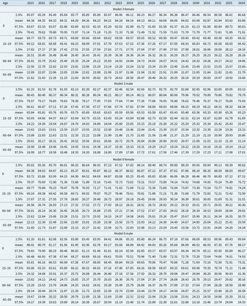
We perform three sets of analyses in this section. The first analysis performs in-sample fitting using all time periods, whereas the second analysis performs out-of-sample forecast using all except the last 20 years to train models and forecast 20 years ahead. These two analyses consider the five selected countries, namely Australia, Iceland, Japan, UK and the US to guide the model selection based on the performance of both in-sample fitting and out-of-sample forecast. The last analysis is our aim to provide life tables for the future 20 years of all 16 countries. This life table analysis uses all data to train models and forecast mortality rates 20 years ahead using traditional LC model (model 3) and the best long memory model (model 8) selected by DIC. We construct the life tables based on mortality rate forecasts using models 3 and 8, without and with a long memory component and compare their performances. We first illustrate the life expectancy calculation in the following section. A substantial set of results, too large for presentation in this manuscript is available in the online technical report accompanying this manuscript, see Yan et al., (Reference Yan, Peters and Chan2018b).
4.1 Life expectancy calculation
4.1.1 Definition of life expectancy
Using the posterior mean of the forecast mortality rates  $ \mu_{x,t}$, we can evaluate the period life expectancy at different ages and construct life tables (Koissi et al., Reference Koissi, Shapiro and Högnôs2006). We consider the same age groups
 $x \in \{0, 1-4, 5-9, \cdots , 95-99\}$ and let
 $\tilde{x}$ to represent the initial age of each age group, that is
 $\tilde x \in \mathcal{S}=\{0, 1, 5, \cdots , 90, 95\}$. Defining further
 $n_{\tilde x}$ as the length of the interval of age group x (corresponds to
 $\tilde x$), we have
 $n_0 = 1, n_1 = 4, n_5 = 5, \cdots , n_{95} = 5$. We then calculate the probability that a person aged
 $\tilde x$ in year t will die in the next
 $n_{\tilde x}$ years as
 \begin{equation*}q_{\tilde x,t}^{n_{\tilde x}}=\frac{n_{\tilde x}\mu_{x,t}}{1+n_{\tilde x}(1-a(\tilde x,n_{\tilde x}))\mu_{x,t}}\end{equation*}
where  $a(\tilde x,n_{\tilde x})$ is the average fraction of the
 $n_{\tilde x}$ years lived by the people who aged initially at
 $\tilde x$ will die during that age interval. Using the assumption that deaths are distributed uniformly in the interval, we set
 $a(\tilde x,n_{\tilde x})=0.5$ for all
 $\tilde x$. The hypothetical number of people
 $l_{\tilde x +n_{\tilde x},t}$ alive at age
 $\tilde x +n_{\tilde x}$ is determined by
 \begin{eqnarray*}l_{\tilde x +n_{\tilde x},t}&=&l_{\tilde x ,t}\left(1-q_{\tilde x,t}^{n_{\tilde x}}\right)=l_{0,t}\prod_{ \left\{k \le \tilde x : k \in \mathcal{S} \right\} }\left(1-q_{k,t}^{n_{k}}\right) \nonumber\end{eqnarray*}
where  $l_{0,t}=100,000$. We can then calculate the number of deaths
 \begin{equation*}d_{\tilde x,t}^{n_{\tilde x}}=l_{\tilde x ,t}-l_{\tilde x +n_{\tilde x},t}=l_{\tilde x ,t}q_{\tilde x,t}^{n_{\tilde x}} \nonumber\end{equation*}
and the person-years lived
 \begin{eqnarray*}L_{\tilde x,t}^{n_{\tilde x}}&=&n_{\tilde x}\left(l_{\tilde x +n_{\tilde x},t}+a(\tilde x,n_{\tilde x})\times d_{\tilde x,t}^{n_{\tilde x}}\right)=n_{\tilde x}l_{\tilde x ,t}\left(1-0.5q_{\tilde x,t}^{n_{\tilde x}}\right) \nonumber\end{eqnarray*}
The total future lifetime of the  $l_{\tilde x ,t}$ people who attain age
 $\tilde x$ is
 $T_{\tilde x ,t}=\sum_{ \left\{j > \tilde x : j \in \mathcal{S} \right\} }L_{j,t}^{n_{\tilde x}}$. Hence, a period life expectancy at age
 $\tilde x$ can be derived by
 \begin{equation}e_{\tilde x ,t}=\frac{T_{\tilde x ,t}}{l_{\tilde x ,t}} \end{equation}
4.1.2 Bayesian approach to life expectancy calculation
According to the definition of life expectancy  $e_{\tilde x ,t}$ in equation (14), we can now obtain a relationship directly between
 $e_{\tilde x ,t}$ and mortality rates
 $\mu_{x,t}$ as
 \begin{equation}e_{\tilde x ,t}=\frac{\sum_{ \left\{j > \tilde x : j \in \mathcal{S} \right\} }n_{j}\left(1-0.5\frac{n_{j}\mu_{j,t}}{1+0.5n_{j}\mu_{j,t}}\right)l_{0,t}\prod_{ \left\{k \le j-n_j : k\in \mathcal{S} \right\} }\left(1-\frac{n_{k}\mu_{k,t}}{1+0.5n_{k}\mu_{k,t}}\right)}{l_{0,t}\prod_{ \left\{ k \le \tilde x-n_{\tilde x } : k \in \mathcal{S} \right\} }\left(1-\frac{n_{k}\mu_{k,t}}{1+0.5n_{k}\mu_{k,t}}\right)} \end{equation}
In order to calculate life expectancy, mortality rates  $\mu_{x,t} $ for all age groups are needed. For calculation convenience, we denote
 ${\boldsymbol{\mu}}_t \in \mathbb{R}^g$ to be a vector of all mortality rates at year t,
 ${\textbf{\textit{e}}}_t \in \mathbb{R}^g$ the corresponding vector for life expectancy and
 $\mathcal{F}_{1:T} $ to be the filtration for all age groups. Therefore, in equation (15), this shows that we can represent the random vector,
 ${\textbf{\textit{e}}}_{t} \in \mathbb{R}^g$, by a vector value transformation of the random mortality rates
 ${\boldsymbol{\mu}}_{t}$, which we denote by
 ${\textbf{\textit{e}}}_{t} =\varrho\!\left( {\boldsymbol{\mu}}_{t} \right)$ with
 $\varrho\,:\, \mathbb{R}^g \rightarrow \mathbb{R}^g $. Each element of the vector function
 $\varrho$ corresponds to a mapping for age group x given by equation (15). We are interested in obtaining the posterior predictive distribution of
 ${\textbf{\textit{e}}}_{T+1\,:\,T+m}$ given
 $\mathcal{F}_{1\,:\,T}$. We first need to obtain the posterior predictive distribution of
 ${\boldsymbol{\mu}}_{T+1\,:\,T+m}$ given
 $\mathcal{F}_{1\,:\,T}$, which is defined as follows:
 \begin{eqnarray} && \hspace*{-25pt}f({\boldsymbol{\mu}}_{T+1\,:\,T+m}|\mathcal{F}_{1\,:\,T}) \nonumber \\
& =& \int \!{\dots}\! \int \prod_{s=1}^{m} \left[f({\boldsymbol{\mu}}_{T+s}({\boldsymbol{\kappa}}_{T+s})|{\boldsymbol{\mu}}_{T+s-1}({\boldsymbol{\kappa}}_{T+s-1}),{\boldsymbol{\vartheta}}, \mathcal{F}_{1\,:\,T}) f({\boldsymbol{\kappa}}_{T+s}|{\boldsymbol{\kappa}}_{T+s-1},{\boldsymbol{\vartheta}}, \mathcal{F}_{1\,:\,T})\right] \nonumber \\
& & \times\ f({\boldsymbol{\mu}}_{1\,:\,T}({\boldsymbol{\kappa}}_{1\,:\,T})| {\boldsymbol{\vartheta}}, \mathcal{F}_{1\,:\,T})f({\boldsymbol{\kappa}}_{1\,:\,T}| {\boldsymbol{\vartheta}}, \mathcal{F}_{1\,:\,T})\pi({\boldsymbol{\vartheta}}|\mathcal{F}_{1\,:\,T}) d {\boldsymbol{\mu}}_{1\,:\,T+m}({\boldsymbol{\kappa}}_{1\,:\,T+m})d {\boldsymbol{\kappa}}_{1\,:\,T+m}d{\boldsymbol{\vartheta}} \end{eqnarray}
Remark 4.1. Equation (16) is an example for autoregressive order 1, which means that  ${\boldsymbol{\mu}}_{T+s}$ only depends on
 ${\boldsymbol{\mu}}_{T+s-1}$.
Our interest is in obtaining the posterior predictive distribution of the life expectancy  ${\textbf{\textit{e}}}_{T+1\,:\,T+m}$ given
 $\mathcal{F}_{1\,:\,T}$. We note the distribution of
 ${\textbf{\textit{e}}}_t$ conditional on
 $\mathcal{F}_{1\,:\,T}$ is then obtained via the following generic expression:
 \begin{eqnarray*} && f_{{\textbf{\textit{e}}}_t}({\textbf{\textit{e}}}_{t}|\mathcal{F}_{1\,:\,t}) = f_{{\boldsymbol{\mu}}_t}(\varrho ^{-1}({\textbf{\textit{e}}}_{t}) |\mathcal{F}_{1\,:\,t}) |J(\varrho({\boldsymbol{\mu}}_{t}))| \nonumber\end{eqnarray*}
where  $f_{{\textbf{\textit{e}}}_t}$ represents the multivariate probability density function (pdf) of life expectancies
 ${\textbf{\textit{e}}}_t $, and
 $f_{{\boldsymbol{\mu}}_t}$ is the multivariate pdf of mortality rates
 ${\boldsymbol{\mu}}_t$. In addition, J is the Jacobian of the transformation
 $\varrho ({\cdot})$ which maps mortality rates to life expectancy according to equation (15). The distribution summaries for the predictive distribution of life expectancy for each age group, such as the marginal mean and variance, can be estimated in Algorithm 1 step 4. In practice, this procedure can be approximated by the Monte Carlo estimator, constructed from posterior samples according to Algorithm 1. Furthermore, unlike the Bayesian filtering which is based on filtration
 $\mathcal{F}_{1\,:\,T}$, the Bayesian smoothing uses also the future measurements for computation. The estimator of states
 $y_{x,t}$ at each time
 $t<T$ conditional on all the measurements up to time T is
 $f(y_{x,t}|\mathcal{F}_{x,1\,:\,T})$ (Särkkä, Reference Särkkä2013). The theorem proposed by Kitagawa (Reference Kitagawa1987) provides the marginal posterior distributions for Bayesian smoothing.
Compute posterior predictive distribution for life expectancy  $f({\textbf{\textit{e}}}_{T+1\,:\,T+m}|\mathcal{F}_{1\,:\,T})$

Theorem 4.1 (The Bayesian smoothing). The Bayesian smoother for computing the smoothed mortality rates distribution  $f({\boldsymbol{\mu}}_{t}|{\boldsymbol{\vartheta}}, \mathcal{F}_{1\,:\,T})$ for any
 $t<T$ is given by the following Bayesian smoothing equation:
 \begin{eqnarray*}f({\boldsymbol{\mu}}_{t}|{\boldsymbol{\vartheta}}, \mathcal{F}_{1\,:\,T})&=&f({\boldsymbol{\mu}}_{t}|{\boldsymbol{\vartheta}}, \mathcal{F}_{1\,:\,t})\int \left [ \frac{f({\boldsymbol{\mu}}_{t+1\,:\,T}({\boldsymbol{\kappa}}_{t+1\,:\,T})|{\boldsymbol{\mu}}_{t}({\boldsymbol{\kappa}}_{t}),{\boldsymbol{\vartheta}} )f({\boldsymbol{\mu}}_{t+1\,:\,T}({\boldsymbol{\kappa}}_{t+1\,:\,T})|{\boldsymbol{\vartheta}}, \mathcal{F}_{1\,:\,T})}{f({\boldsymbol{\mu}}_{t+1\,:\,T}({\boldsymbol{\kappa}}_{t+1\,:\,T})|{\boldsymbol{\vartheta}}, \mathcal{F}_{1\,:\,t})} \right ] \nonumber \\[4pt]
& & \times f({\boldsymbol{\kappa}}_{1\,:\,T}|{\boldsymbol{\vartheta}}, \mathcal{F}_{1\,:\,T})d{\boldsymbol{\mu}}_{t+1\,:\,T}({\boldsymbol{\kappa}}_{t+1\,:\,T}) d {\boldsymbol{\kappa}}_{1\,:\,T}\end{eqnarray*}
where  $f({\boldsymbol{\mu}}_{t+1\,:\,T}({\boldsymbol{\kappa}}_{t+1\,:\,T})|{\boldsymbol{\vartheta}}, \mathcal{F}_{1\,:\,t})$ is the predictive distribution defined in equation (16).
Since the Bayesian smoothing of life expectancy  $f(e_{\tilde x,t}|\mathcal{F}_{x,1\,:\,T})$ can be calculated by mortality rates
 $\mu_{x,t}$, the smoothed posterior distribution of life expectancy
 $e_{\tilde x ,t}$ is given by Algorithm 1.
Data length and abbreviation for country names

4.2 Mortality data
The mortality data sets of 16 countries are downloaded from the HMD, which provides detailed mortality and population data to the public. Table 3 reports the data size for each country together with its abbreviated name.
Each data set contains the number of deaths  $y_{x,t}^*$ and the exposure
 $E_{x,t}^*$ cross-classified by genders and years and they are aggregated into 21 age groups, namely age 0 group, age 1–4 groups, age 5–10 groups, age 11–15 groups, etc. Values of
 $y_{x,t}^*$ and
 $E_{x,t}^*$ are scaled according to the following equation (17):
 \begin{equation}y_{x,t}=[y_{x,t}^*/c_x] \ \ \mbox{and} \ \ E_{x,t}=E_{x,t}^*/c_x \end{equation}
where  $[{\cdot}]$ represents rounding to the nearest integer, and the scaling factor
 $c_x$ is determined by
 \begin{equation*}c_x=10^k \ \ \mbox{if} \ \ \underset{t}{\min} \ y_{x,t}^* \in \left(10^{k+1},10^{k+2}\right)\end{equation*}
such that the range of  $y_{x,t}$ is approximately within (0,100) and k is an integer selected to achieve this. This re-scaling of data only changes the unit and preserves the data features. In other words, if the number of deaths
 $y_{x,t}^*$ and the exposure
 $E_{x,t}^*$ are scaled by the same amount
 $c_x$, the features of data will maintain. This can be explained by following equation (18):
 \begin{equation}\mathbb E\left(y_{x,t}^*/c_x|E_{x,t}^*\right)\approx \mathbb E\left(\left[y_{x,t}^*/c_x\right]|E_{x,t}^*\right)=E_{x,t}^*\mu_{x,t}/c_x=E_{x,t}\mu_{x,t} \end{equation}
Furthermore, we find comprehensively statistically significant evidence for the presence of long memory features, which are present irrespective of how the data sets are aggregated or disaggregated. To illustrate this, we take Australia female death count as an example. There are different ways to aggregate age groups. For example, taking five age groups for each way, one can form single age  $\{0, 1, 2, 3, 4\}$ for type 1 or alternatively
 $\{0, 1-4, 5-9, 10-14, 15-19\}$ for type 2 or
 $\{0-10, 11-20, 21-30, 31-40, 41-50\}$ for type 3. However, since some features like weak correlation in a time series may be diminished or removed via aggregation, we need to test if the persistence in the form of long memory that exists in the data will also be reduced or eliminated by aggregation. To do this, we apply Hurst exponent H (Hurst, Reference Hurst1951), a non-parametric measure of long memory, to measure the strength of long memory for the three types of aggregation. Davidson & De Jong (Reference Davidson and De Jong2000) demonstrated the simple relationship
 $d = H - 0.5$ between d and H, confirming the role of H to measure the strength of long memory in a given time series. Table 4 shows that the estimated H are similar across the three types of aggregation, testifying the prevalence of long memory as a structural feature in aggregation typically.
Estimated Hurst exponent for three types of aggregation. Age group differs across different types of aggregation, for example, age group 2 for Type 1 is 1, for Type 2 is 1–4 and for Type 3 is 11–20

Estimated  $d_x$ (first row) and
 $u_x$ (second row) using female (first two rows) and male (next two rows) death counts fitted by model 6 for the five selected countries. The estimated value of
 $u_x$ for Iceland female in the last age group is 0.08313 and for Iceland male in the last two age groups are
 $-0.03799$ and
 $-0.07389$. For US male, the last reading is 0.9875.

5. In-Sample Fitting
We study three important model components, namely long memory, LC structure and graduation, in our proposed model and demonstrate how different model components capture some data features for the five selected countries. These components are crucial to capture the attributes of different mortality models discussed in section 1.1. For instance, the period effect is addressing the LC model structure and the graduation component is addressing a smooth trend variation. The new long memory structure is adopted to capture the long memory feature in mortality data, which is discussed in section 2.3. To study each component independently of the others, we consider model 6, model 3 and model 1 in Table 2, which contain parameters ( $d_x$,
 $u_x$),
 $\eta_x$ and
 $\mathbb{B}_x(t;\ 0,l,{\boldsymbol{\tau}})$ alone, respectively, apart from the general level parameter
 $\alpha_x$. We also compare the goodness of fit for the eight models and use DIC to select the best fitting model for each mortality data set. Furthermore, the difference between the mortality rates smoothed by each model and the mortality rates from HMD are evaluated by MAEs, RMSEs, MAPEs and MASEs defined in section 3.2 to provide additional guidelines in model selection. Then, the best model is used to provide estimates of mortality rates and then life expectancies for the five selected countries.
Long memory features using model 6: The estimated  $d_x$ and
 $u_x$ are obtained from model 6, which is a GLGARMA model containing only a long memory component. The first two rows in Figure 4 describe the estimated values of
 $d_x$ and
 $u_x$ for females and the next two rows for males. For females, Iceland data shows much less pronounced memory properties (lower
 $d_x$), especially for older age groups. All the other four countries illustrate long memory because the estimates of
 $d_x$ are close to
 $0.5$. The estimates of
 $u_x$ for these five countries are all close to 1 except for the older age groups in Iceland. These results suggest that the majority of mortality data follow ARFIMA type long memory rather than Gegenbauer-type long memory. For males, the strength of long memory in Iceland again is weaker, especially in older age groups. For both females and males in Iceland, the estimated values of
 $d_x$ in the last age group are very low, which may give imprecise estimates of
 $u_x$ because the long memory features of a weak long memory time series are difficult to distinguish from white noise.
Estimated  $\eta_x$ for period effect when death counts of the five selected countries are fitted using model 3 for female (first row) and male (second row). The estimated value of
 $\eta_x$ for Iceland female in the last age group is 0.5351 and for male, the last two values are 0.5975 and
 $-0.03941$.

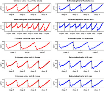
Estimated spline coefficients  $a_{x,i}^{(0)}$ for 21 age groups in each of the l stages by fitting five countries death counts for female (left) and male (right) using model 1. Each block in each plot represents a stage of 20 years in which the coefficient is assumed to be consistent. The first row is for Australia, followed by Iceland, Japan, UK and US.

DIC of the eight models fitted to death counts of the five countries by gender. Each model type is represented by dots in the order of 21 age groups.

Period effect using model 3: The estimates of parameter  $\eta_x$ in the AR term describe the stationarity condition for period effect. As a basic period effect model, model 3 is selected to explore the features of
 $\eta_x$. Figure 5 shows that the estimated values of
 $\eta_x$ for females and males are close to 1, which means the period effect tends to be non-stationary to capture the trend. For both females and males, the estimated values of
 $\eta_x$ in the last age group are much lower, especially for Iceland. This suggests the mortality rates for the last age group tend to be stable with very marginal improvement in longevity despite the substantial advancement in medical health over the years.
Pattern of graduation effects using model 1: The estimated coefficients  $a_{x,i}^{(0)}$ for the
 $\mathbb{B}_x(t;\ 0,l,{\boldsymbol{\tau}})$ spline in model 1 are plotted in Figure 6. Each stage represents a consistent mortality level for a period of 20 years and this length of 20 years is chosen to ensure enough information to estimate the coefficient in each stage to a desirable level of accuracy. Due to the difference in data length, the five countries have different numbers of stages. All of these graphs illustrate the general pattern across age groups that in each stage, the estimated
 $a_{x,i}^{(0)}$ declines from age 0 to the lowest level around the age of 10–14 and then increases. This pattern of changes of
 $a_{x,i}^{(0)}$ during a life cycle follows a decreasing trend over the years and confirms the improvements in living and medical conditions for the five selected countries.
Model fit for all models using DIC : Figure 7 depicts DIC values across age groups for models in Table 2. For countries with long memory features, such as Australia, Japan, UK and US, the performance of models incorporating a long memory component is significantly enhanced (lower DIC) compared to short memory models (models 1–4; without long memory structures). For Iceland data with a short memory, the short memory models are better than long memory models.
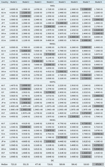
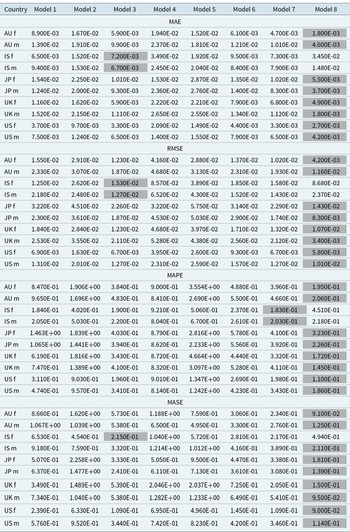
Table 5 shows the performance of the eight models using four selection criteria, namely MAEs, RMSEs, MAPEs and MASEs defined in section 3.2 by comparing the estimated mortality rates  $\hat{\mu}_{x,t}$ with the observed
 $\mu_{x,t}$ from HMD. Generally speaking, long memory models (models 5–8) perform better than short memory models. Model 8 is the best fitted model as it has the greatest number of highlights (the lowest criteria across a row) in Table 5 as well as the overall lowest median DIC of 476.56.
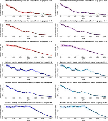
In-sample mortality rate estimates using models 3 and 8: In order to visualise the enhanced performance of model 8 as compared with the traditional LC model (model 3), Figure 8 as an example plots the time series of observed and fitted mortality rates, each superimposed with their 95% credible intervals for three age groups (10–14, 40–45 and 65–69) representing youth, middle-aged and senior for female and male, respectively, in Australia. The plots of estimated mortality rates for Iceland, Japan, UK and US are listed in the Appendix of Yan et al., (Reference Yan, Peters and Chan2018b). The performance of model 8 with long memory structure is much better than model 3 as model 8 can fit the trend and capture the peaks of the time series better in general. All mortality rates show a decreasing trend over the years. The drop seems to be faster before 1950 (WW2) and slower with levelling off thereafter for the youth and middle-aged groups but it shows an opposite trend with a convex (instead of concave) shape for the senior group. This shows that the improvement of mortality is faster for the youth and middle-aged groups in earlier years but after 1950, the improvement in the senior group is more obvious which possibly benefits from the further advancement in medical services. For the UK, it is interesting to see that model 8 can capture the small peak of increased mortality during the time of World War Two (WW2) better. Model 8 also gives narrower confidence intervals indicating a more precise estimation. In comparing mortality rates across countries, Iceland has more variation over the years and wider confidence intervals possibly due to its small population size. The trend of mortality rates also displays more variation for males and for the US.
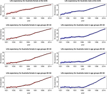
In-sample life expectancy estimates using model 8: As model 8 clearly provides more accurate mortality rate estimates, it is chosen to estimate life expectancy for the five selected countries. Figure 9 graphs the life expectancy of Australia calculated using the mortality rate estimates from model 8 for both genders and four selected age groups. The plots of the estimated life expectancy for Iceland, Japan, UK and US are given in the Appendix of Yan et al., (Reference Yan, Peters and Chan2018b). The plots display a linear increasing trend across years for females at a younger age but a sharper increase after 1966 for middle and senior age groups. This sharper increase pattern is more noticeable for male particularly at a senior age. The plots also show close agreement with the life expectancies calculated using the observed mortality rates from HMD. So we can conclude that the performance of in-sample life expectancy estimates is satisfactory.
Four selection criteria and DIC to measure the accuracy of estimated  $\hat{\boldmath{\mu}}_{x,1\,:\,T}$ for five selected countries

Note: the best models amongst models 1-8 are shaded by light grey colour.
Observed mortality rate  $\mu_{x,t}$ (black line) from HMD and estimated mortality rate
 $\hat{\mu}_{x,t}$ by model 8 (left) and model 3 (right) for female (red and purple) and male (blue and sky blue) for the three age groups (10–14, 40–45 and 65–69) in Australia.

Observed life expectancy  $e_{\tilde x ,t}$ (black line) from HMD and life expectancy calculated using the estimated mortality rates from model 8 (red in female and blue in male) for both female (left) and male (right) and four age groups (0, 20–24, 40–44 and 60–64) in Australia.

5.1 Out-of-sample forecasting
In order to measure the forecast performance of the eight models, the number of death counts  ${\textbf{\textit{Y}}}_{x,1\,:\,T}$ by 21 age groups and both genders of the 5 selected countries are each divided into 2 parts, the training
 ${\textbf{\textit{Y}}}_{x,1\,:\,(T-20)}$ and forecast
 ${\textbf{\textit{Y}}}_{x,(T-19)\,:\,T}$ for years 1994 to 2014. Similar to Table 5 , Table 6 reports the four criteria that compare the mortality rate forecasts
 $\hat{{\boldsymbol{\mu}}}_{x,(T-19)\,:\,T}$ with the observed from HMD for the eight models. Model 8 again provides the best forecasts in all except seven cases coming from Iceland in which five cases favour model 3 as Iceland data has a short memory.
To view the improved forecast performance of model 8 compared with model 3, Figure 10 plots the time series of observed  ${\boldsymbol{\mu}}_{x,T-19\,:\,T}$ from HMD and the forecasted
 $\hat{{\boldsymbol{\mu}}}_{x,T-19\,:\,T}$ using model 3 and model 8 with 95% credible interval for the young, middle and senior age groups, respectively. The forecast performance of model 8 with a long memory component is much better than the traditional LC model (model 3) because the mortality rate forecasts are closer to the observed and have sharper credible intervals, which enclose the observed mortality rates. Moreover, the traditional LC model consistently overestimates the mortality rate.
Figure 11 displays the 20-step ahead forecasts of Australia life expectancy using model 8 for both genders and 4 age groups (0, 20–24, 40–44 and 60–64).
The performance of out-of-sample life expectancy forecasts is also reasonable as the forecasted values are close to the life expectancies calculated using observed mortality rates from HMD and these “observed” life expectancies are contained within the credible interval.
A range of additional forecast results for mortality rates and life expectancies for Iceland, Japan, UK and the US is provided in Yan et al., (Reference Yan, Peters and Chan2018b). This includes further analysis of the four model performance criteria for the forecasted number of deaths  $\widehat{{\textbf{\textit{Y}}}}_{x,(T-19)\,:\,T}$ using all the eight models.
Four selection criteria to measure the accuracy of forecast  $\hat{{\boldsymbol{\mu}}}_{x,(T-19)\,:\,T}$ for the five selected countries

Note: the best models amongst models 1-8 are shaded by light grey colour.
Observed mortality rates  ${\boldsymbol{\mu}}_{x,T-19\,:\,T}$ (black line) from HMD and forecasted
 $\hat{{\boldsymbol{\mu}}}_{x,T-19\,:\,T}$ by model 3 (female in purple and male in skyblue) and model 8 (female in red and male in blue) for both female (first row) and male (second row) and three age groups (10–14, 35–39 and 70–74) in Australia.

Observed life expectancy  $e_{\tilde x ,t}$ from HMD (black line) and life expectancy calculated using the forecasted mortality rates from model 8 (red in female and blue in male) for female (first row) and male (second row) and four age groups (0, 20–24, 40–44 and 60–64) in Australia.

The forecasted Australia life expectancy by model 3 and model 8

5.2 Life expectancy of 16 countries forecasted 20 years ahead
In this analysis, we calculate life expectancy based on the 20 years ahead of forecasts of mortality rates for 16 countries using model 8, the best performing model in the previous 2 analyses and model 3, the LC model for comparison. Table 7 reports the life table forecast for selected age groups 0, 15 – –19, 60 – –69 in Australia using model 3 and model 8. The life expectancy for all 16 countries and all age groups are given in Yan et al., (Reference Yan, Peters and Chan2018b).
The trend of life expectancy forecast is slowly increasing over the forecast period for all age groups, gender and models. Compared with model 3, the life expectancy forecast using model 8 is higher consistently for all age groups, gender and years.
6. Conclusion
This paper explores the long memory features in mortality data and the impacts of this stylised factor on the construction of the life table. It is demonstrated in this work that classical GLM regression models in mortality forecasting can be naturally extended to incorporate different forms of long memory persistence time series structure within the family of GLARMA regression models. A Bayesian modelling approach is successfully applied and shown to outperform equivalent Bayesian GLM LC mortality regression models not incorporating long memory structure when it comes to both in-sample and out-of-sample forecasting model performance.
A comprehensive data analysis is undertaken to incorporate mortality records for 16 countries mortality data sets. It is demonstrated that in all cases the model incorporating long memory features consistently outperforms equivalent types of models with no such structure and this is consistent for all age groups and genders. In order to foster a deeper understanding of how the long memory features improve the mortality model fitting and forecasting performance, we propose a generalised model (model 8) including a spline component, a period effect component and a long memory component.
Moreover, we perform simulation studies to assess the accuracy of the parameter estimates of model 8 and seven sub-models. The core reference model that we use in benchmark comparison is the univariate LC model (model 3) with a stochastic period effect. The extended models which incorporate the graduation model, period effect, and long memory effect are compared with this LC model (model 3). We perform this study in a range of different structural component changes, which produces seven different models. The model with the most structure is model 8 which contains a graduation effect, a period effect, and a long memory effect in a stochastic trend. Compared with other sub-models including the univariate LC model (model 3), model 8 is the best model and is selected from the studies of in-sample fitting and out-of-sample forecasting. The enhancement in life expectancy forecasts is also demonstrated by comparing results from model 8 with model 3. In addition, the life expectancy forecasts 20 years ahead for 16 countries using model 8 and model 3 are reported with credible intervals. There are some limitations to our current study. Unlike multivariate models, our proposed model cannot capture the cohort effect.
The implications of these findings for practitioners in particular is that when aiming to forecast mortality accurately, rather than resorting to a non-stationary stochastic period effect or period-cohort effect model, it is statistically more accurate to instead consider stationary models which incorporate long memory structure. This will, in turn, improve in-sample fit and more importantly reduce bias in out-of-sample forecast performance. In turn, reduction of the bias will result in more accurate life table constructions and then fairer calculations of life insurance premiums and greater accuracy in product pricing.
Appendix
A. Simulation Studies
The accuracies of parameter estimates for each model are assessed by a series of simulation studies to validate the accuracy of the estimation techniques we develop for the proposed models. In each study, we consider eight sub-models as given in Table 2. All simulated data for each model are generated by the same seed, and we adopt four different lengths of data, namely  $n_1=100$,
 $n_2=150$,
 $n_3=250$ and
 $n_4=550$. We purposely choose a large data size of
 $n_4=550$ to verify if some inaccuracies in parameter estimates are due to insufficient sample size. Moreover, true parameter values are chosen to generate death counts in a similar magnitude to the observed rescaled death counts, often in the range of 0–250.
Case study A.1. Parameter accuracy across levels of  $d_x$ and
 $u_x$.
In this case study, we first focus on model 8 which is the full model consisting of  $\mathbb{B}_x(t;\ 0,l,{\boldsymbol{\tau}})$ spline, period effect and long memory effect. The B-spline
 $\mathbb{B}_x(t;\ r,l, {\boldsymbol{\tau}})$ is of order r with l knot points
 ${\boldsymbol{\tau}}=(\tau_1,\ldots,\tau_l)$. We compare the effect of varying levels of
 $u_x$ (indicates the period of oscillatory ACF) and
 $d_x$ (strength of long memory) on the parameter accuracy. We also consider the parameter accuracy when
 $u_x$ is negative which gives instantaneous oscillatory ACF or anti persistence.
According to the results in Table A.1, there are two main findings. First, the accuracy of parameter estimates will get worse when the strength of long memory becomes weaker because the oscillatory features in the ACF are difficult to distinguish from the white noise in the model. Second, the parameter estimates are much less accurate even with a moderate data size ( $n_3=250$) if
 $u_x$ is negative. However, this problem can be improved when the data size increases to
 $n_4=550$. Results suggest that negative
 $u_x$ is harder to estimate and so larger sample size is needed to obtain reasonable estimates of
 $u_x$ and other parameters. However, as all
 $u_x$ are estimated to be positive for the mortality data we study in this paper, the problem with estimating a negative
 $u_x$ is not an issue in our studies.
True values, estimates and credible intervals for parameters  $d_x$ and
 $u_x$ using model 8

True values, estimates and credible intervals for parameters  $\eta_x$ in models 3 and 7 with data length
 $n_1$,
 $n_2$ and
 $n_3$ when
 $d_x=0.45$ and
 $u_x=0.9$ for both models 3 and 7

True values, estimates and credible intervals for parameters  $a_{x,1}^{(0)}$ of model 1 with data length
 $n_1$ and
 $S=10$, of model 4 with data length
 $n_1$ and of model 8 with data length
 $n_2$,
 $d_x=0.45$ and
 $u_x=0.9$

Four selection criteria to measure the accuracy of the 20 steps ahead forecasts using models 3, 4 and 7 with different data sizes when  $u_x=0.9$,
 $\eta_x=0.5$ and
 $\mathbb{B}_x(t;\ 0,l,{\boldsymbol{\tau}})=-5$

Note: the best models amongst models 3, 4 and 7 are shaded by light grey colour.
Case study A.2. Accuracy of AR parameter in period effect
The parameter  $\eta_x$ of the AR term in the period effect describes a stationary period process if
 $|\eta_x|<1$. The results in Table A.2 compares the accuracy of parameter estimate
 $\eta_x$ in models 3 and 7. For model 3,
 $\eta_x$ can be estimated to a reasonable level of accuracy with the smallest data size of
 $n_1=100$. However, after adding the long memory structure to model 7, it can only be properly estimated with larger data sizes of
 $n_2=150$ and
 $n_3=250$. Results show that the accuracy will decrease with increasing model complexity (model 7). Again, this issue can be solved by increasing the sample size and a sample size of 150 was tested to provide reasonable estimates of
 $\eta_x$ for model 7. Although the accuracy for negative
 $\hat{\eta}_x$ is not as promising as those of the positives,
 $\hat{\eta}_x$ in our data analysis are again consistently positive.
Case study A.3. Accuracy of spline function parameters
The spline function  $\mathbb{B}_x(t;\ 0,l,{\boldsymbol{\tau}})$ allows the intercepts
 $a_{x,i}^{(0)}$ in
 $\mu_{x,t}$ to remain fixed in each stage i of S data points marked by knot points
 $(\tau_i,\tau_{i+1}) \in {\boldsymbol{\tau}}$ and to vary across stages. Hence it provides level information for the death rate in each stage of the data set. Table A.3 reports the spline parameter estimates
 $a_{x,1}^{(0)}$ across stage length S for models 1, 4 and 8 which contain the spline components
 $\mathbb{B}_x(t;\ 0,l,{\boldsymbol{\tau}})$ in the mean function. The table shows that the accuracy of
 $a_{x,1}^{(0)}$ can be improved by increasing S rather than data size in general because the longer stage will provide more data information to estimate the parameters in the spline function better. As the simplest model, model 1 in Table A.3 shows that it provides accurate parameter estimates for the smallest data of size 100 with each stage containing only
 $S=10$ data points. However, with more complicated model structures,
 $a_{x,i}^{(0)}$ are highly sensitive to initial values and prior distributions. This estimating issue can be solved by increasing S. Taking model 4 with data length
 $n_1=100$ in Table A.3 as an example, the estimate of
 $a_{x,1}^{(0)}$ is reasonable when
 $S=30$. However, if we only increase the data length to
 $n_2=150$ but use a shorter stage length of
 $S=10$, the estimate of
 $a_{x,1}^{(0)}$ is around -3 (not reported in the table) which is very inaccurate. For model 8,
 $S=40$ data points in each stage will be sufficient to estimate
 $a_{x,1}^{(0)}$ accurately. Furthermore, model 1, as the simplest form of graduation model, provides reasonable estimates with small sample size (
 $n_1=100$) and moderate number of knot points such that each stage contains approximately 10 data points. However, for more complicated model, such as models 4 and 8, the stage length for each stage needs to increase to
 $S = 30$ and
 $S = 50$, respectively, to provide sufficient information for reasonably accurate estimates.
Case study A.4. Accuracy of forecasts with model misspecification
Model specification is also an important factor in model selection. Given an ARMA(1,1) model,
 \begin{equation*}Y_{t+1}=c+\phi Y_{t}+\varepsilon _{t+1}-\theta \varepsilon _{t}, \nonumber\end{equation*}
the one-step ahead forecast  $\hat{y}_{t+1}$ can be represented as
 \begin{equation*}\widehat{Y}_{t+1}=c+\phi Y_{t}+0-\theta \varepsilon _{t},\nonumber\end{equation*}
since  $\hat{\varepsilon }_{t+1}=0$ and the variance of forecast error is
 \begin{equation*}\mathbb{V}\mbox{ar}(Y_{t+1}-\widehat{Y}_{t+1})=\mathbb{V}\mbox{ar}(\varepsilon_{t+1})=\sigma^2. \nonumber\end{equation*}
For ARFIMA(1, d, 1) model,
 \begin{equation*}Y^{\prime}_{t+1}=c+\phi Y^{\prime}_{t}+(1-B)^{-d}\left ( \varepsilon _{t+1}-\theta \varepsilon _{t} \right ), \nonumber\end{equation*}
and the one-step ahead forecast  $\hat{y}_{t+1}$ can be represented as
 \begin{equation*}\widehat{Y}^{\prime}_{t+1}=c+\phi Y^{\prime}_{t}-(1-B)^{-d}\theta \varepsilon _{t}, \nonumber\end{equation*}
where the long memory component  $(1-B)^{-d}$ with range
 $|\varphi_j|<1$ is
 \begin{equation*}(1-B)^{-d} =\sum_{j=0}^{\infty }\frac{\Gamma (j+d)}{\Gamma (j+1)\Gamma (d)}B^{j} =\sum_{j=0}^{\infty }\varphi _{j}B^j . \nonumber\end{equation*}
Hence, the variance of forecast error is given by
 \begin{equation*}\mathbb{V}\mbox{ar}(Y^{\prime}_{t+1}-\widehat{Y}^{\prime}_{t+1})=\mathbb{V}\mbox{ar}((1-B)^{-d}\varepsilon _{t+1})=\left(1+\sum_{j=1}^{\infty }\varphi _{j}^2 \right)\sigma^2 ,\nonumber\end{equation*}
where  $(1+\sum_{j=1}^{\infty }\varphi _{j}^2 )$ is a positive number greater than 1. Consequently, the variance of forecast error
 $\mathbb{V}\mbox{ar}(Y^{\prime}_{t+1}-\widehat{Y}^{\prime}_{t+1})$ is much greater than
 $\mathbb{V}\mbox{ar}(Y_{t+1}-\widehat{Y}_{t+1})$. The presence of long memory in most mortality data has been studied in Yan et al., (Reference Yan, Peters and Chan2018a). This shows that for a model with misspecification by dropping the long memory model, the variance of model parameters will be underestimated. Consequently, we aim to investigate how this model misspecification affects the forecast accuracy. We first simulate data from model 7 with period effect and long memory and forecast 20-step ahead for
 $m = 20$ time points using models 3, 4 and 7 with different data size
 $n_1$,
 $n_3$ and
 $n_4$. We note that models 3 and 4 contain period effects but with no long memory component. To facilitate comparison, we vary the levels of
 $d_x$ which indicate different strengths of long memory. The forecasts
 $\hat{y}_{x;\ T+s}$ are estimated using the posterior mean of the posterior sample described in equation (10). The four selection criteria, namely MAE, RMSE, MAPE and MASE are used to assess the forecast accuracy. Table A.4 shows that the forecast performance of model 3 and 4 gets worse with a higher level of d and larger data size, in general, as the discrepancy between the true and fitted models is larger and clearer, respectively. Model 7 with long memory component is much better than the other two models even with small sample size
 $n_1 = 100$ and the performance of model 3 improves with a larger sample size. Overall, model 7 with a long memory component is preferred when the data show long memory features.