1 Introduction
Buoyant jets or forced plumes often occur in natural environment and engineering applications. The ambient into which the buoyant jets are discharged is in many cases turbulent (background turbulence). Examples include a buoyant effluent jet from an ocean outfall discharging into coastal waters, or a human-generated thermal plume releasing into a ventilated room.
The presence of background turbulence will generally affect the mixing characteristics of a buoyant jet. The large eddies of the background will cause the jet to meander and increase its absolute spread rate, and the small eddies with size comparable to the jet length scale can alter or even destroy the jet structure if their velocity scales are also comparable (Kiya, Ohyama & Hunt Reference Kiya, Ohyama and Hunt1986). This has been observed experimentally in momentum jets (Law, Cheng & Davidson Reference Law, Cheng and Davidson2001; Guo et al. Reference Guo, Malcangio, Davies and Fernando2005), buoyant jets (Cuthbertson et al. Reference Cuthbertson, Malcangio, Davies and Mossa2006) and plumes (Ching, Fernando & Robles Reference Ching, Fernando and Robles1995; Hubner Reference Hubner2004), all in oscillating-grid-generated turbulence.
The turbulence intensity generated by an oscillating grid decays nonlinearly with distance from the grid, and the integral length scale grows as the turbulence decays (Cheng & Law Reference Cheng and Law2001). Close to the grid, the turbulence is strongest, but its strength quickly diminishes along the distance from the grid. A jet discharging opposite to the grid will thus encounter a turbulence field with increasing intensity away from the source, so the jet would break up abruptly close to the grid. The inhomogeneous turbulence used in past experiments made it difficult to reach consistent conclusions among different studies and generalize results. Recently, with the use of a random-jet-array turbulence generator, Variano & Cowen (Reference Variano and Cowen2008) and Khorsandi, Gaskin & Mydlarski (Reference Khorsandi, Gaskin and Mydlarski2013) were able to carry out experiments of pure jets discharging into a reasonably homogeneous and isotropic turbulence (HIT) field. The measurements showed that before the breakup point, the spread rate of the jet increased, and axial velocity decreased relative to a jet in quiescent ambient. Interestingly, the jet momentum defined by the mean jet mixing characteristics was found to be no longer conserved but decreased along the downstream distance – an observation that is counterintuitive as there are no external net forces acting on the jet.
It is of interest to predict the change in jet mixing characteristics due to the background turbulence before breakup, especially the change in jet entrainment rate for the modelling of the buoyant jet. However, conclusions as to how background turbulence affects the jet entrainment rate are inconsistent in the literature. Hubner (Reference Hubner2004) suggested that the background turbulence would increase the entrainment rate of a plume, and together with the meandering effects of the large eddies would lead to an increased spreading rate. A similar suggestion was made by Wright (Reference Wright, Davies and Valente Neves1994), who proposed that free-stream turbulence would increase the entrainment of the jet, but the experimental data were too scattered to arrive at a solid conclusion. Although the increased jet spread would intuitively lead to a suggestion of increased entrainment, theoretical arguments and recent experimental measurements have indicated the reverse. Hunt (Reference Hunt, Davies and Valente Neves1994) and Hunt, Eames & Westerweel (Reference Hunt, Eames and Westerweel2006) argued theoretically that the increasing momentum that is transported by the jet turbulence (instead of the mean flow) causes the entrainment to decrease. The reduction in entrainment was later also observed experimentally by Khorsandi et al. (Reference Khorsandi, Gaskin and Mydlarski2013) for a pure momentum jet.
In terms of modelling, Hubner (Reference Hubner2004) developed an integral model of a plume in background turbulence by incorporating the ‘increase’ in entrainment due to the background turbulence, and achieved some success in the plume-width prediction. However, as argued by Hunt (Reference Hunt, Davies and Valente Neves1994) and observed by Khorsandi et al. (Reference Khorsandi, Gaskin and Mydlarski2013), the entrainment will in fact decrease; it is thus difficult to justify the model based on physical grounds. It is also not trivial to generalize the model to a buoyant jet with both source momentum and buoyancy fluxes. Other models such as those of Hunt (Reference Hunt, Davies and Valente Neves1994), Ching et al. (Reference Ching, Fernando and Robles1995) and Cuthbertson et al. (Reference Cuthbertson, Malcangio, Davies and Mossa2006) focused more on the prediction of the jet or plume breakup point, and should be addressed separately.
In summary, there is hitherto no physically sound model that is able to predict quantitatively the mixing characteristics of a buoyant jet in background HIT. Thus, the main objective in this study is to develop a general predictive model of a buoyant jet in background HIT. In this paper, we first present the theory, dimensional analysis and the proposed integral model of a buoyant jet in background HIT in § 2. Then, the experimental set-up of this study, which involves a random jet array background turbulence generator and a buoyant jet discharge apparatus, is presented in § 3. In § 4, both the first- and second-order turbulence statistics of a jet were measured, which enables us to examine the conservation of momentum flux for a pure momentum jet, and compare with literature findings. Comparisons were also made between the integral model predictions and experimental observations. In § 5, the integral model predictions and experimental observations for a buoyant jet are presented. Discussion of the implications from the predictions of the model and some applications are then given in § 6, followed by the conclusion of this study in § 7.
2 Theory
2.1 Governing equations
Consider an axisymmetric turbulent buoyant jet without swirl in a field of background HIT with zero mean flow. The Reynolds-averaged governing equations in cylindrical coordinates (axial direction
 $z$
, radial direction
 $r$
and azimuthal direction
 $\unicode[STIX]{x1D703}$
) of continuity, axial and radial momentum (in conservative form) and the tracer mass conservation are given by
 $$\begin{eqnarray}\displaystyle & \displaystyle \frac{\unicode[STIX]{x2202}\overline{w}}{\unicode[STIX]{x2202}z}+\frac{1}{r}\frac{\unicode[STIX]{x2202}r\overline{u}}{\unicode[STIX]{x2202}r}=0, & \displaystyle\end{eqnarray}$$
 $$\begin{eqnarray}\displaystyle & \displaystyle \frac{\unicode[STIX]{x2202}(\overline{w}^{2}+\overline{w^{\prime 2}})}{\unicode[STIX]{x2202}z}+\frac{1}{r}\frac{\unicode[STIX]{x2202}}{\unicode[STIX]{x2202}r}r(\overline{u}~\overline{w}+\overline{u^{\prime }w^{\prime }})=-\frac{1}{\unicode[STIX]{x1D70C}}\frac{\unicode[STIX]{x2202}\overline{P}}{\unicode[STIX]{x2202}z}+g\frac{\overline{\unicode[STIX]{x0394}\unicode[STIX]{x1D70C}}}{\unicode[STIX]{x1D70C}}, & \displaystyle\end{eqnarray}$$
 $$\begin{eqnarray}\displaystyle & \displaystyle \frac{\unicode[STIX]{x2202}(\overline{u}~\overline{w}+\overline{u^{\prime }w^{\prime }})}{\unicode[STIX]{x2202}z}+\frac{1}{r}\frac{\unicode[STIX]{x2202}}{\unicode[STIX]{x2202}r}r(\overline{u}^{2}+\overline{u^{\prime 2}})=-\frac{1}{\unicode[STIX]{x1D70C}}\frac{\unicode[STIX]{x2202}\overline{P}}{\unicode[STIX]{x2202}r}+\frac{\overline{v}^{2}}{r}, & \displaystyle\end{eqnarray}$$
 $$\begin{eqnarray}\displaystyle & \displaystyle \overline{u}\frac{\unicode[STIX]{x2202}\overline{c}}{\unicode[STIX]{x2202}r}+\overline{w}\frac{\unicode[STIX]{x2202}\overline{c}}{\unicode[STIX]{x2202}z}=-\frac{1}{r}\frac{\unicode[STIX]{x2202}r\overline{u^{\prime }c^{\prime }}}{\unicode[STIX]{x2202}r}-\frac{\unicode[STIX]{x2202}\overline{w^{\prime }c^{\prime }}}{\unicode[STIX]{x2202}z}. & \displaystyle\end{eqnarray}$$
In the above equations,
 $(u,v,w)$
corresponds to the velocity components in the (
 $r$
,
 $\unicode[STIX]{x1D703}$
,
 $z$
) directions,
 $g$
is the acceleration due to gravity (acting in the
 $-z$
direction),
 $\unicode[STIX]{x1D70C}_{a}$
is the ambient density and
 $\unicode[STIX]{x0394}\unicode[STIX]{x1D70C}=\unicode[STIX]{x1D70C}-\unicode[STIX]{x1D70C}_{a}$
is the local density difference. An overline represents time averaging and a prime represents the velocity or concentration fluctuation about the mean. The viscous diffusion terms have been neglected since they are negligible away from solid boundaries for high-Reynolds-number flows (Hussein, Capp & George Reference Hussein, Capp and George1994). Following Hussein et al. (Reference Hussein, Capp and George1994), integration of the radial momentum equation with respect to
 $r$
from
 $r$
to infinity, substituting the
 $z$
-derivative of pressure into the
 $z$
-momentum equation, and integrating over the entire jet cross-section will result in the conservation equation of total momentum flux:
 $$\begin{eqnarray}\displaystyle 2\unicode[STIX]{x03C0}\frac{\text{d}}{\text{d}z}\int _{0}^{\infty }[\overline{w}^{2}+\overline{w^{\prime 2}}-\overline{u^{\prime 2}}]r\,\text{d}r=2\unicode[STIX]{x03C0}\int _{0}^{\infty }g\frac{\overline{\unicode[STIX]{x0394}\unicode[STIX]{x1D70C}}}{\unicode[STIX]{x1D70C}}r\,\text{d}r+\underbrace{2\unicode[STIX]{x03C0}[r(\overline{u}\overline{w}+\overline{u^{\prime }w^{\prime }})]_{0}^{\infty }}_{=0\text{ for HIT}}. & & \displaystyle\end{eqnarray}$$
It has been assumed that
 $\overline{u^{\prime 2}}\approx \overline{v^{\prime 2}}$
, as observed in a buoyant jet in quiescent ambient (Wang & Law Reference Wang and Law2002); this is reasonable when the jet structure has not been significantly altered by the background turbulence, as is the region of interest in this study. Also note that the shear stress, mean flow and the
 $z$
-gradient of the root-mean-square (r.m.s.) velocity of the background HIT are zero when
 $r\rightarrow \infty$
, which results in an equation with the second-order terms (the turbulence contribution) that is exactly the same as that of a buoyant jet in quiescent ambient (Wang & Law Reference Wang and Law2002).
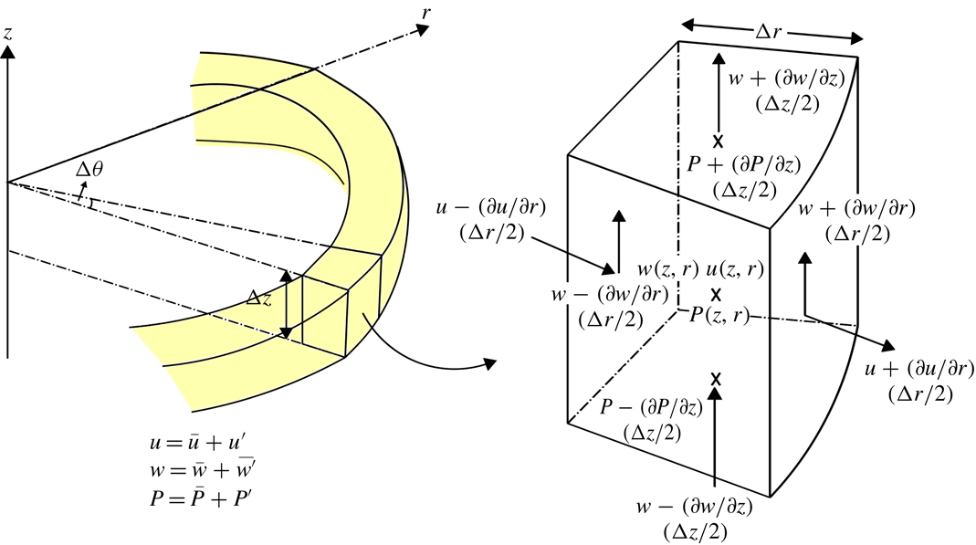
Equation (2.5) can also be arrived at using control volume (CV) analysis. Equation (2.2) is a result of the
 $z$
-momentum balance of the ring-shape CV as shown in figure 1 (see appendix A). The lateral net
 $z$
-momentum flux into the CV is represented by the term
 $(1/r)(\unicode[STIX]{x2202}/\unicode[STIX]{x2202}r)r(\overline{u}\overline{w}+\overline{u^{\prime }w^{\prime }})$
, which includes the shear stress
 $\overline{u^{\prime }w^{\prime }}$
. Noting that the shear stress is identically zero in HIT (e.g. Pope Reference Pope2000) external to the jet and that
 $\overline{u^{\prime }w^{\prime }}$
is equal and opposite for positive and negative
 $\unicode[STIX]{x1D703}$
within the jet, the net contribution of the term to the
 $z$
-momentum balance of the CV is hence zero (note that this is not so for other types of turbulence). Integrating the remaining terms in the momentum balance equation along
 $r$
from 0 to
 $\infty$
, and noting that
 $(1/\unicode[STIX]{x1D70C})\unicode[STIX]{x2202}_{z}\overline{P}\approx -\unicode[STIX]{x2202}_{z}\overline{u^{\prime 2}}$
(e.g. Hussein et al.
Reference Hussein, Capp and George1994 and Shabbir & George Reference Shabbir and George1994), will result in (2.5).
Control volume of a buoyant jet in background HIT.

In equation (2.5), the left-hand side represents the rate of change of total momentum
 $M$
in the jet direction, which consists of the momentum flux contributed by the mean flow,
 $$\begin{eqnarray}\displaystyle M_{M}=2\unicode[STIX]{x03C0}\int _{0}^{\infty }\overline{w}^{2}r\,\text{d}r, & & \displaystyle\end{eqnarray}$$
and that contributed by the turbulence or the second-order terms,
 $$\begin{eqnarray}\displaystyle M_{T}=2\unicode[STIX]{x03C0}\int _{0}^{\infty }[\overline{w^{\prime 2}}-\overline{u^{\prime 2}}]r\,\text{d}r. & & \displaystyle\end{eqnarray}$$
The right-hand side represents the local buoyancy force, which increases the total momentum of the buoyant jet along
 $z$
. In quiescent ambient, the ratio of
 $M_{T}$
to
 $M$
is typically only about 10 % (Papanicolaou & List Reference Papanicolaou and List1988), and a first-order integral model that gives good predictions of the jet mixing characteristics can be developed by considering only the momentum flux contributed by the mean flow (Lee & Chu Reference Lee and Chu2003). However, with background turbulence, it is expected that the relative contribution of turbulent momentum flux will become progressively more important (Hunt et al.
Reference Hunt, Eames and Westerweel2006) and needs to be considered.
The tracer mass conservation equation (2.4) can also be integrated to give the mass conservation equation in integral form as
 $$\begin{eqnarray}\displaystyle 2\unicode[STIX]{x03C0}\frac{\text{d}}{\text{d}z}\int _{0}^{\infty }(\overline{wc}+\overline{w^{\prime }c^{\prime }})r\,\text{d}r=0, & & \displaystyle\end{eqnarray}$$
and the total tracer mass flux
 $H$
can similarly be expressed as the sum of the contribution from the mean flow
 $$\begin{eqnarray}\displaystyle H_{M}=2\unicode[STIX]{x03C0}\int _{0}^{\infty }\overline{wc}r\,\text{d}r & & \displaystyle\end{eqnarray}$$
and that from the turbulence
 $$\begin{eqnarray}\displaystyle H_{T}=2\unicode[STIX]{x03C0}\int _{0}^{\infty }\overline{w^{\prime }c^{\prime }}r\,\text{d}r. & & \displaystyle\end{eqnarray}$$
It is useful to define two variables to represent the ratios of the total to the mean fluxes of momentum
 $(k_{M})$
and tracer mass
 $(k_{H})$
as in Wang & Law (Reference Wang and Law2002), where
 $$\begin{eqnarray}\displaystyle k_{M}=1+\frac{M_{T}}{M_{M}} & & \displaystyle\end{eqnarray}$$
and
 $$\begin{eqnarray}\displaystyle k_{H}=1+\frac{H_{T}}{H_{M}}. & & \displaystyle\end{eqnarray}$$
The radial velocity and concentration profiles of a buoyant jet in background turbulence are in general not self-similar, but are expected to be Gaussian in shape initially (after the zone of flow establishment
 ${\approx}6D$
(Fischer et al.
Reference Fischer, List, Koh, Imberger and Brooks1979; Lee & Chu Reference Lee and Chu2003)) until the jet structure becomes severely affected by the background HIT (not considered in this study). If we consider the region in which the velocity and concentration profiles are Gaussian, i.e.
 $$\begin{eqnarray}\displaystyle \overline{w}=\overline{w_{c}}\exp [-(r/b_{g})^{2}]\quad \text{and}\quad \overline{c}=\overline{c_{c}}\exp [-(r/\unicode[STIX]{x1D706}b_{g})^{2}], & & \displaystyle\end{eqnarray}$$
where
 $b_{g}$
is the Gaussian jet half-width, defined as the radial distance from the jet centreline in which the velocity has decayed to
 $\exp (-1)$
of
 $\overline{u_{c}}$
, and
 $\unicode[STIX]{x1D706}\approx 1.0{-}1.2$
(Wood, Bell & Wilkinson Reference Wood, Bell and Wilkinson1993) is the ratio of the jet concentration Gaussian half-width to velocity Gaussian half-width, then a set of integral equations can be developed by integrating (2.1), (2.5) and (2.8) (replacing
 $c$
by
 $g\unicode[STIX]{x0394}\unicode[STIX]{x1D70C}/\unicode[STIX]{x1D70C}$
), and using the entrainment hypothesis (Morton, Taylor & Turner Reference Morton, Taylor and Turner1956):
 $$\begin{eqnarray}\displaystyle & \displaystyle \frac{\text{d}Q}{\text{d}z}=2\unicode[STIX]{x1D6FC}\sqrt{\frac{2\unicode[STIX]{x03C0}M}{k_{M}}}, & \displaystyle\end{eqnarray}$$
 $$\begin{eqnarray}\displaystyle & \displaystyle \frac{\text{d}M}{\text{d}z}=\frac{k_{M}}{k_{H}}(1+\unicode[STIX]{x1D706}^{2})\frac{FQ}{2M}, & \displaystyle\end{eqnarray}$$
 $$\begin{eqnarray}\displaystyle & \displaystyle \frac{\text{d}F}{\text{d}z}=0, & \displaystyle\end{eqnarray}$$
where
 $Q$
,
 $M$
and
 $F$
are the total volume, momentum and buoyancy fluxes, respectively;
 $\unicode[STIX]{x1D6FC}$
is the entrainment coefficient which is
 $\unicode[STIX]{x1D6FC}_{j}=0.057$
for a jet to
 $\unicode[STIX]{x1D6FC}_{p}=0.086$
for a plume (e.g. Wang & Law Reference Wang and Law2002), and varied for a buoyant jet as, for example,
 $\unicode[STIX]{x1D6FC}=\unicode[STIX]{x1D6FC}_{j}+(\unicode[STIX]{x1D6FC}_{p}-\unicode[STIX]{x1D6FC}_{j})(Fr_{p}/Fr_{L})^{2}$
, where
 $Fr_{p}=(5/4)^{1/2}(\unicode[STIX]{x1D706}/\sqrt{2})$
and
 $Fr_{L}=w_{c}/\sqrt{g^{\prime }b_{g}}$
are the plume and local densimetric Froude numbers, respectively (Lee & Chu Reference Lee and Chu2003). Note that the second-order statistics of the jet are not self-similar even for the range of
 $z/l_{c}$
considered in this study, but the effects due to the change in their cross-sectional profiles on the jet mixing characteristics have been accounted for via
 $k_{M}$
and
 $k_{H}$
. Also, the background turbulence is expected to change the entrainment coefficient derived from a quiescent background since the turbulence kinetic energy (TKE) production is enhanced and the turbulence statistics profiles are also changing downstream (see van Reeuwijk & Craske Reference van Reeuwijkl and Craske2015 for a detailed derivation and discussion of the entrainment coefficient). Our preliminary analysis showed that the change in
 $\unicode[STIX]{x1D6FC}$
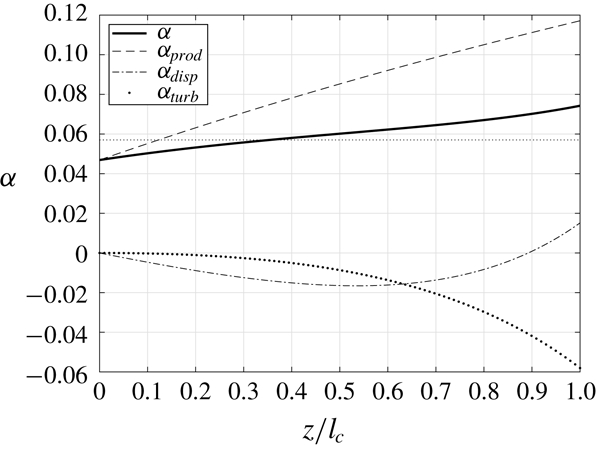
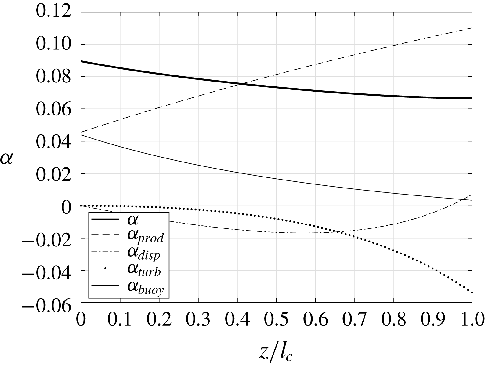
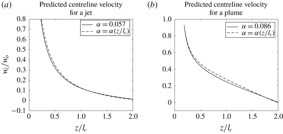
has a maximum of about 20 % in our region of interest and the model predictions are relatively insensitive to this change (see appendix B); hence the entrainment coefficient for a quiescent background will be adopted in this study until a devoted study on the issue is available. The centreline variables of the buoyant jet can be calculated by relating them to the fluxes:
 $$\begin{eqnarray}\displaystyle \overline{w_{c}}=\frac{2M}{k_{M}Q},\quad b_{g}=\sqrt{\frac{k_{M}Q^{2}}{2\unicode[STIX]{x03C0}M}}\quad \text{and}\quad \frac{\unicode[STIX]{x0394}\unicode[STIX]{x1D70C}}{\unicode[STIX]{x1D70C}}g=\frac{(1+\unicode[STIX]{x1D706}^{2})}{k_{H}\unicode[STIX]{x1D706}^{2}}\frac{F}{Q}. & & \displaystyle\end{eqnarray}$$
The effect of background HIT can be introduced into the integral equations through
 $k_{M}$
and
 $k_{H}$
. The two variables generally depend on the flow characteristics of both the jet and the background turbulence, as demonstrated in the following dimensional analysis.
2.2 Dimensional analysis
To simplify the problem, dimensional analysis is carried out to identify the key dimensionless parameters. The buoyant jet under consideration can be characterized by its initial volume
 $(Q_{o})$
, momentum
 $(M_{o})$
and buoyancy
 $(F_{o})$
fluxes. The background turbulence can be characterized by its r.m.s. velocity
 $u_{a}^{\prime }$
and dissipation rate
 $\unicode[STIX]{x1D716}_{a}$
. Then any dependent variables
 $\unicode[STIX]{x1D719}$
of the jet can be expressed as a function of
 $$\begin{eqnarray}\displaystyle \unicode[STIX]{x1D719}\sim f(Q_{o},M_{o},F_{o},z,u_{a}^{\prime },\unicode[STIX]{x1D716}_{a}). & & \displaystyle\end{eqnarray}$$
The choice of variables to characterize can be further explained. Following Hunt (Reference Hunt, Davies and Valente Neves1994), only the smaller scales of the background turbulence can affect the jet; larger eddies can only meander the jet without affecting its structure. Thus, while the r.m.s. velocity
 $u_{a}^{\prime }$
and integral length scale
 $L_{I}$
are intuitively more relevant quantities to characterize the background turbulence, the velocity scale
 $u^{\prime }<u_{a}^{\prime }$
of the background turbulence with length scale/eddy size
 $L$
close to that of the jet
 $L\sim L_{J}<L_{I}$
is more the key in affecting the jet/plume structure, where
 $L_{J}$
is the jet/plume characteristic length scale. When
 $u^{\prime }\sim u_{J}$
, the jet structure will be severely affected, where
 $u_{J}$
is the buoyant jet characteristic velocity. This critical velocity scale
 $u^{\prime }$
can be estimated as
 $u^{\prime }\sim (L\unicode[STIX]{x1D716}_{a})^{1/3}\sim (L_{J}\unicode[STIX]{x1D716}_{a})^{1/3}\sim (\unicode[STIX]{x1D6FD}z\unicode[STIX]{x1D716}_{a})^{1/3}$
, where
 $\unicode[STIX]{x1D6FD}$
is the jet spread rate. This occurs when
 $z\sim u^{\prime 3}/\unicode[STIX]{x1D716}_{a}$
and thus it is sensible to use
 $\unicode[STIX]{x1D716}_{a}$
in characterizing the background turbulence. The second variable to characterize the background turbulence can be
 $u_{a}^{\prime }$
or
 $L_{a}$
. The significance of
 $u_{a}^{\prime }/w_{o}$
has been described by Ching et al. (Reference Ching, Fernando and Robles1995) and will be adopted in this study. If
 $u_{a}^{\prime }/w_{o}\gg 1$
, it is possible for the jet/plume to break up at the onset. On the other hand, if
 $u_{a}^{\prime }/w_{o}\ll 1$
as in this study, the jet/plume will travel to a certain distance before breaking up. It is hence another parameter of physical significance and should be included.
One possible set of dimensionless groups from (2.18) is
 $$\begin{eqnarray}\displaystyle \unicode[STIX]{x1D719}^{\prime }\sim f\left[\frac{Q_{o}\unicode[STIX]{x1D716}_{a}^{5/6}}{F_{o}^{7/6}},\frac{M_{o}\unicode[STIX]{x1D716}_{a}^{2/3}}{F_{o}^{4/3}},\frac{z}{(M_{o}^{3}/\unicode[STIX]{x1D716}_{a}^{2})^{1/8}},\frac{u_{a}^{\prime }}{(F_{o}\unicode[STIX]{x1D716}_{a})^{1/6}}\right]. & & \displaystyle\end{eqnarray}$$
But a more useful set is found by combining the dimensionless groups
 $$\begin{eqnarray}\displaystyle \unicode[STIX]{x1D719}^{\prime }\sim f\left(Fr,\frac{z}{l_{M}},\frac{z}{l_{c}},\frac{u_{a}^{\prime }}{w_{o}}\right). & & \displaystyle\end{eqnarray}$$
In equation (2.20),
 $Fr\sim M_{o}^{5/4}/F_{o}^{1/2}Q_{o}$
is the jet densimetric Froude number and
 $l_{M}\sim M_{o}^{3/4}/F_{o}^{1/2}$
is the momentum length scale; when
 $z/l_{M}<\sim 1$
, the flow is momentum-dominated (a jet), and when
 $z/l_{M}>\sim 6$
it becomes buoyancy-dominated (a plume). Parameter
 $l_{c}$
is the critical length scale in which the jet will start to be severely affected by the background turbulence. The physical significance of
 $l_{c}$
was first noticed by Hunt (Reference Hunt, Davies and Valente Neves1994), who argued that when the velocity scale of the background eddies with size comparable to the jet width is close to that of the jet entrainment velocity, the jet structure will begin to be severely affected by the background turbulence. A theoretically derived relationship showed that
 $l_{c}=l_{cp}=(F_{o}/\unicode[STIX]{x1D716}_{a})^{1/2}$
for a plume (Hunt Reference Hunt, Davies and Valente Neves1994), while for jets,
 $l_{c}=l_{cj}=(M_{o}^{3}/\unicode[STIX]{x1D716}_{a}^{2})^{1/8}$
(see appendix C). It is expected that when
 $z\ll l_{c}$
, the jet mixing will not be significantly affected, while when
 $z\gg l_{c}$
, the jet mixing will be noticeably affected, or even be broken up by the turbulence. In the transition regime, the change in jet mixing characteristics has to be measured. Finally, the term
 $u_{a}^{\prime }/w_{o}$
indicates that, in general, with the same
 $z/l_{c}$
, the jet may still be affected by the ratio of the jet initial velocity and the background turbulence intensity. The importance of
 $u_{a}^{\prime }/w_{o}$
(if any) is to be determined experimentally. It can be seen there for pure jets, equation (2.20) can be simplified to
 $$\begin{eqnarray}\displaystyle \unicode[STIX]{x1D719}^{\prime }\sim f\left(\frac{z}{l_{cj}},\frac{u_{a}^{\prime }}{w_{o}}\right); & & \displaystyle\end{eqnarray}$$
and for pure plumes, equation (2.20) can be simplified to
 $$\begin{eqnarray}\displaystyle \unicode[STIX]{x1D719}^{\prime }\sim f\left(\frac{z}{l_{cp}}\right). & & \displaystyle\end{eqnarray}$$
In this study, for buoyant jets in which
 $1<z/l_{M}<5$
, whether
 $l_{cj}$
or
 $l_{cp}$
is more appropriate in the interpretation of experimental data will be discussed. Also, the importance of
 $u_{a}^{\prime }/w_{o}$
will be determined using the data of our experiments as well as those in the literature; the variation of the buoyant jet mixing characteristics with
 $z/l_{c}$
will be measured. In particular, the determination of
 $k_{M}$
and
 $k_{H}$
along
 $z/l_{c}$
will enable a predictive integral model to be formulated.
3 Experiments
3.1 Experimental set-up
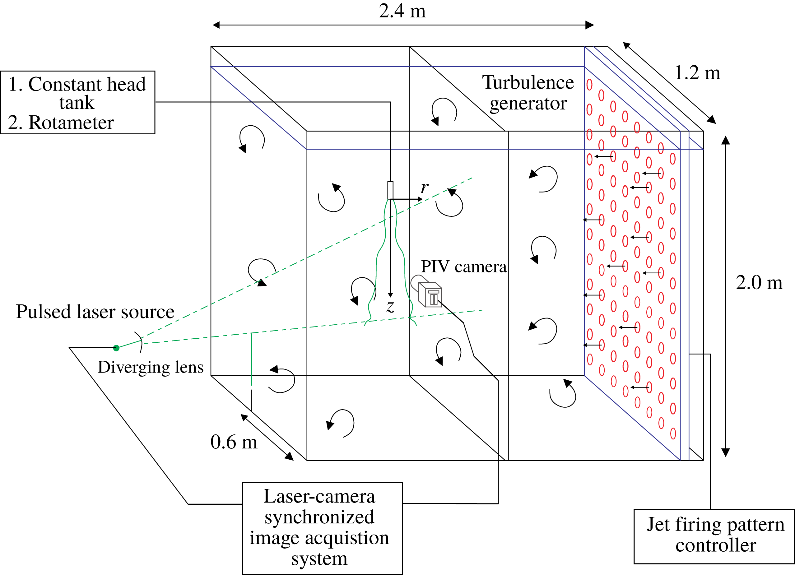
In order to investigate how buoyant jet mixing characteristics vary with the different dimensionless parameters in a background HIT, laboratory experiments were carried out using a tank which was 2.4 m (long)
 $\times$
1.2 m (wide)
 $\times$
2.0 m (deep) (figure 2). The ambient turbulence was generated by a ‘randomly actuated synthetic jet array’ (RASJA; Variano & Cowen Reference Variano and Cowen2008; Khorsandi et al.
Reference Khorsandi, Gaskin and Mydlarski2013) mounted at one end of the tank. This turbulence generator can be moved along the length of the tank so that the distance between the measurement point and the generator can be adjusted (usually for the purpose of adjusting the turbulence intensity at the measurement point). The generator consisted of 12 rows, each with 8 bilge pumps, and a PVC tube of diameter 2.1 cm was mounted on each pump as a jet nozzle. The centre-to-centre distance between nozzles was
 $S=15~\text{cm}$
. The pumps were controlled by a computer and could be switched on and off using two algorithms: (i) the ‘coin-toss’ algorithm – in which a jet is assigned a probability of being turned on at each predetermined time step and (ii) the ‘sunbathing’ algorithm – in which each jet is controlled independently with a random on time and off time with normal distribution
 $(\unicode[STIX]{x1D707}_{on},\unicode[STIX]{x1D70E}_{on})$
and
 $(\unicode[STIX]{x1D707}_{off},\unicode[STIX]{x1D70E}_{off})$
, respectively. Algorithm (ii) was found to perform better by Variano & Cowen (Reference Variano and Cowen2008) and was hence adopted in this study. The distributions were chosen to be
 $(\unicode[STIX]{x1D707}_{on},\unicode[STIX]{x1D70E}_{on})=(12,4)$
s and
 $(\unicode[STIX]{x1D707}_{off},\unicode[STIX]{x1D70E}_{off})=(108,36)$
s, similar to that used in Khorsandi et al. (Reference Khorsandi, Gaskin and Mydlarski2013). The details of the overall turbulence statistics generated by our turbulence generator will be reported separately. The integral length scale
 $L_{I}$
near the jet discharge was calculated by integrating the area under the spatial autocorrelation function–distance curve of the r.m.s. velocity measured, and was found to be
 $L_{11}=L_{L}=8.8~\text{cm}$
and
 $L_{33}=L_{T}=6.8~\text{cm}$
, with an average of
 $L_{I}=7.8~\text{cm}$
. The dissipation rate
 $\unicode[STIX]{x1D716}_{a}$
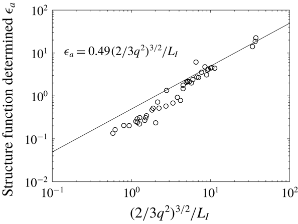
was determined by the scaling law (Variano & Cowen Reference Variano and Cowen2008):
 $$\begin{eqnarray}\displaystyle \unicode[STIX]{x1D716}_{a}=\frac{A(2/3q^{2})^{3/2}}{L_{I}}, & & \displaystyle\end{eqnarray}$$
where
 $q$
is the TKE and
 $A$
is an experimental constant. The constant
 $A=0.49$
was obtained in our background turbulence experiments by comparing the dissipation rate obtained by structure function fit and the scaling law shown in figure 3 (following the method described by Variano & Cowen Reference Variano and Cowen2008), which will be reported in detail in a separate publication.
Experimental set-up of a negatively buoyant jet in quiescent ambient.

The dissipation rates obtained by the structure function against that obtained by the scaling law.

For this study, a test region in the tank with a nearly isotropic and homogeneous turbulent background with negligible mean flow was desired, which can be achieved if the region of interest was located far enough from the turbulence generator where the rate of change of turbulence intensity is smaller along
 $x$
. We chose
 $x=11.5S$
in this study, where
 $x$
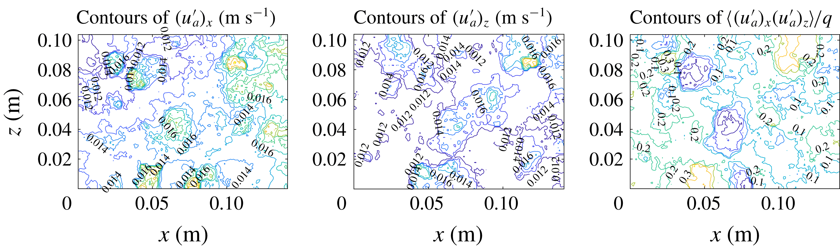
is the distance from the RASJA. Supplementary jet background turbulence experiments were carried out at the jet discharge location for each series of buoyant jet experiments; the r.m.s. velocity and the shear stress of these experiments were ensemble averaged, and the resulting contour maps of these quantities are shown in figure 4. The spatially averaged background r.m.s. velocity components were determined as
 $[(u_{a})_{x},(u_{a})_{z}]=(0.0142,0.0132)$
. The r.m.s. velocity was
 $u_{a}^{\prime }=\sqrt{2/3q^{2}}=0.0135~\text{m}~\text{s}^{-1}$
, where
 $q^{2}=1/2[(u_{a}^{\prime })_{x}^{2}+2(u_{a}^{\prime })_{z}^{2}]$
is the TKE. The mean flows
 $\overline{(u_{a})_{x}}$
and
 $\overline{(u_{a})_{z}}$
were small compared to the r.m.s. velocity (table 1).
The turbulence decay length scale (Maxey Reference Maxey1987)
 $L_{decay}=q^{2}/(\text{d}q^{2}/\text{d}x)\approx 70~\text{cm}$
at
 $x=11.5S$
, and
 $L_{I}/L_{decay}\approx 0.1$
which was effectively homogeneous (Variano & Cowen Reference Variano and Cowen2008) and sufficient for this study. As a measure of the isotropy of the background turbulence considered, we calculated the ratio
 $(u_{a}^{\prime })_{x}/(u_{a}^{\prime })_{z}=1.075$
. The spatially averaged normalized shear stress
 $\overline{(u_{a}^{\prime })_{x}(u_{a}^{\prime })_{z}}/q=0.13$
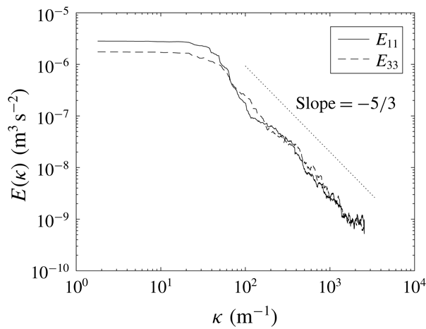
was close to the ideal value of 0. However, from the one-dimensional spectra of a point near to the jet measurements (figure 5), the energy-containing motions were not perfectly isotropic, the same as other studies of RASJA (Variano & Cowen Reference Variano and Cowen2008). The integral length scale ratio
 $L_{11}/L_{33}=1.29$
was different from 2, which can be calculated from the theory of three-dimensional HIT (Pope Reference Pope2000). This reflects that inhomogeneity and anisotropy existed in the flow. A summary of the turbulence characteristics of this study is given in table 1; the overall characteristics were measurements that scattered over a region of 0.7 m (long)
 $\times$
0.4 m (wide)
 $\times$
1.0 m (tall), while those at the jet background were regions of 14 cm (long)
 $\times$
10 cm (tall).
Contour maps of various ensemble-averaged turbulence statistics of the jet background turbulence experiments.

One-dimensional spectra of a point close to the jet measurement.

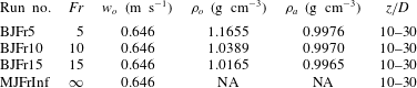
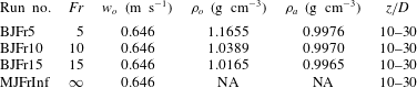
A turbulent vertical (negatively) buoyant saline water jet was discharged into the field of turbulence from a nozzle with internal diameter
 $D=1.0~\text{cm}$
and initial velocity
 $w_{o}=0.646~\text{m}~\text{s}^{-1}$
(flow driven by gravity using a constant-head tank and controlled by a calibrated rotameter), giving a Reynolds number of 6460 which should be sufficiently large for a turbulent jet at the onset. The measured density of the ambient fresh water
 $\unicode[STIX]{x1D70C}_{a}$
was about
 $0.997~\text{g}~\text{cm}^{-3}$
, while the saline jet had densities
 $\unicode[STIX]{x1D70C}_{j}=1.0165~\text{g}~\text{cm}^{-3}$
,
 $1.0389~\text{g}~\text{cm}^{-3}$
and
 $1.1655~\text{g}~\text{cm}^{-3}$
in three different series of experiments, giving
 $Fr=5$
, 10 and 15. Experiments of pure momentum jets with the same density of the ambient were also carried out, and enabled us to compare our measurements with those of past similar studies (Khorsandi et al.
Reference Khorsandi, Gaskin and Mydlarski2013). A summary of the experimental parameters used in this study is given in table 2.
Summary of the background turbulence characteristics.

Buoyant jet discharge parameters.
Particle image velocimetry (PIV) was used to measure the instantaneous velocity field of the buoyant jet. The source fluid and the ambient were first seeded with Dantec
 $50~\unicode[STIX]{x03BC}\text{m}$
diameter polyamid seeding particles. A Dantec DualPower 100-100 laser was used to generate laser pulses at 2
 $\times$
100 mJ with a wavelength of 532 nm. A laser guide arm was used for alignment of the pulsed laser light sheet generated from the laser head with divergence angle of
 $33^{\circ }$
. A complementary metal–oxide semiconductor camera (Dantec SpeedSense 1040, 2320
 $\times$
1726 pixels, 14 cm
 $\times$
10 cm field of view) was placed perpendicularly to, and synchronized with, the pulsed laser sheet to capture the resulting PIV images. The PIV image pairs were sampled at 50 Hz with pulsed laser sheets separated by
 $5000~\unicode[STIX]{x03BC}\text{s}$
, with a maximum storage duration of 20 s.
In each series of jet experiments, measurements were made separately at distances of
 $z=10D{-}20D$
and
 $z=20D{-}30D$
due to the limitation of the field of view of the camera. The laser sheet was aligned to cut through the centreline plane of the jet. Experiments of a buoyant jet in quiescent ambient were first carried out as reference cases. The jet was then discharged into the field of background turbulence and the resulting PIV images were captured. For the distance of
 $z=10D{-}20D$
, 10 ensembles each of 20 s duration were captured; 20 ensembles were captured for the distance of
 $z=20D{-}30D$
since the jet was more affected by the HIT and less steady downstream. The jets of some runs were observed to be meandered outside of the field of view, but we did not have enough statistics to justify whether this is a part of the physics or unintended flow resulting from the less than ideal background HIT (e.g. non-zero mean flow), so we opted to include all these data in the analysis.
To determine the velocity vectors, the PIV images were subdivided into interrogation windows of size 32
 $\times$
32 pixels. An adaptive-correlation method was used to determine the velocity vectors in the windows based on 50 % overlapping using the DynamicStudio software from Dantec Dynamics. This resulted in an instantaneous velocity vector map with 106
 $\times$
144 vectors. The first- and second-order statistics of each point were then derived from the instantaneous velocity maps. Note that when the refractive index of the jet is not the same as that of the ambient, the images of individual particles will be blurred, causing possible error in the PIV measurements. Zhang, He & Jiang (Reference Zhang, He and Jiang2017) attempted to assess the impact of the refractive-index mismatch in a plume experiment, and found that this had insignificant impact on the mean and turbulence statistics of the plume. We have also compared our experimental results (first- and second-order statistics) of a buoyant jet in quiescent ambient with the well-established measurements of previous studies to ensure the measurements were reliable.
3.2 Buoyant jets in quiescent ambient
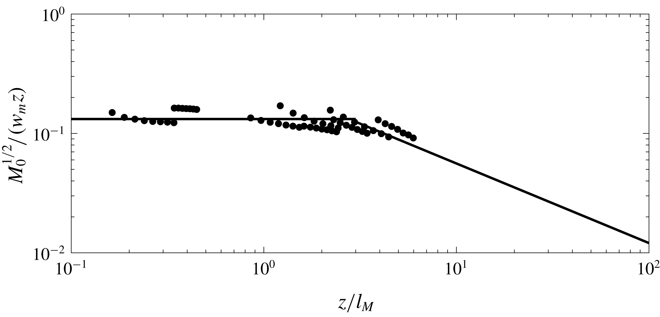
Experiments of the mixing of a buoyant jet in quiescent ambient served to ensure the reliability of the measurement techniques by comparing with data in the literature. The time-averaged centreline velocity of the buoyant jet with
 $Fr=5,10,15$
, as well as that of a momentum jet were extracted and are given in figure 6. It has been observed that when
 $z/l_{M}<\sim 1$
, the normalized centreline velocity
 $\sqrt{M}/(w_{m}z)$
is a constant. When
 $z/l_{M}>\sim 6$
, the normalized velocity
 $\sqrt{M}/(w_{m}z)\sim (z/l_{M})^{-2/3}$
. Our experimental data fell mainly in the transition regime,
 $1<z/l_{M}<5$
, and the centreline velocity can be seen to follow the best-fit curve of Papanicolaou & List’s (Reference Papanicolaou and List1988) experimental data, ranging between the jet regime and the plume regime. The jet Gaussian half-widths
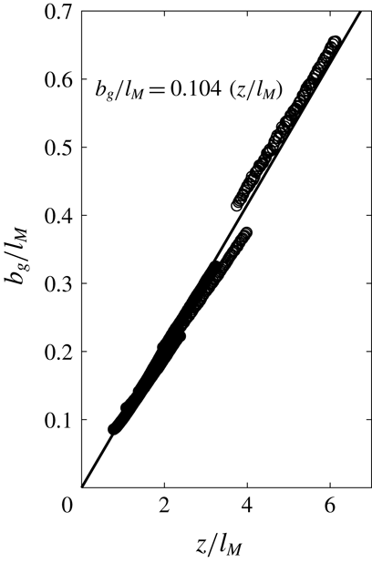
 $b_{g}$
were measured and are plotted against the downstream distance
 $z$
in figure 7. The spread rate of the buoyant jet was measured to be 0.104, which is consistent with the spread rate measured by Wang & Law (Reference Wang and Law2002), and within the range of jet spread rate in the literature summarized by Fischer et al. (Reference Fischer, List, Koh, Imberger and Brooks1979).
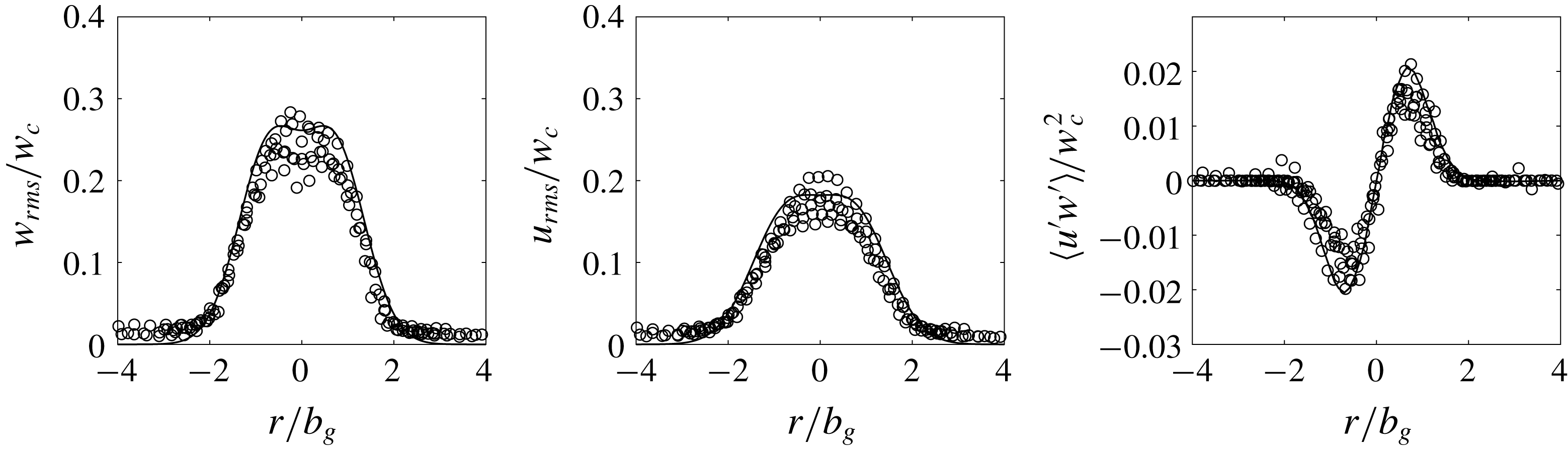
The second-order statistics of the buoyant jet were extracted from the PIV images. The turbulence intensity of the axial and radial velocity, and also the normalized shear stress are plotted in figure 8. The statistics are in general consistent with those measured by Wang & Law (Reference Wang and Law2002). The turbulence intensity of the axial velocity has a peak value of 0.20–0.30, and that of the radial velocity is slightly lower, ranging from 0.15 to 0.20. The shear stress is also consistent with that measured by Papanicolaou & List (Reference Papanicolaou and List1988) and Wang & Law (Reference Wang and Law2002). External to the jet, the shear stress is zero; inside of the jet, the normalized shear stress peaks at about 0.02, and by symmetry it is zero at the centre of the jet. Overall, our measurements are consistent with those in the literature, showing the reliability of our measurement techniques.
Normalized centreline velocity of a buoyant jet. The line represents the best fit of Papanicolaou & List’s (Reference Papanicolaou and List1988) data.

The growth of Gaussian jet width of a buoyant jet with distance measured in this study.

Normalized second-order statistics of a buoyant jet. The solid line represents the best fit of Wang & Law’s (Reference Wang and Law2002) data.

4 Pure jets in background turbulence
4.1 Observation
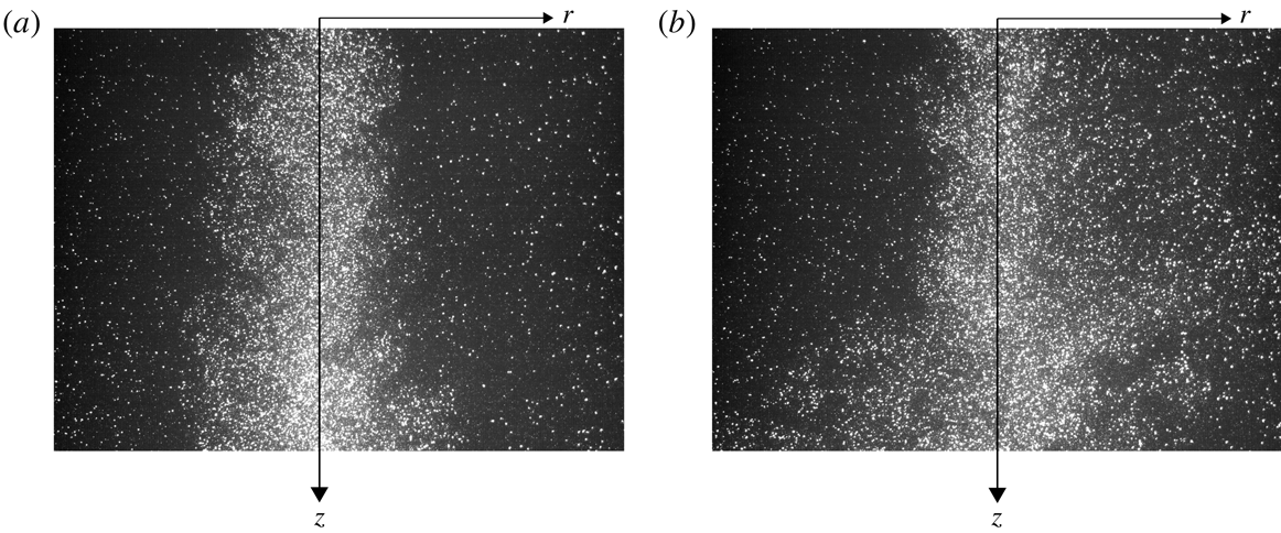
Figure 9 shows a typical jet in quiescent ambient and background turbulence. With background turbulence, the jet can be seen to meander due to the large background eddies. The smaller eddies of the background turbulence appeared to have been incorporated into the jet, dispersing the jet further. Occasionally, there would be a sudden strong eddy acting on the jet and advecting it out of the field of view. This tended to occur more frequently at further downstream distances, as the jet velocity decayed and was more easily affected by the turbulence. The meandering and dispersion by the background eddies affected noticeably the mixing of the buoyant jet, and the effects will be presented quantitatively in the next subsection.
Visualization of a jet in (a) quiescent ambient and (b) background turbulence at
 $z=10D{-}20D$
.

4.2 Mixing characteristics
Khorsandi et al. (Reference Khorsandi, Gaskin and Mydlarski2013) presented the experimental results of the mixing characteristics of a jet in background turbulence. It was observed that the jet centreline velocity decayed faster when the background turbulence intensity increased, or when the jet Reynolds number decreased. It is well known that the centreline velocity of a jet in quiescent ambient, when normalized by the initial jet velocity, will decay with downstream distance as
 $w_{m}/w_{o}\propto (z/D)^{-1}$
(Fischer et al.
Reference Fischer, List, Koh, Imberger and Brooks1979; Lee & Chu Reference Lee and Chu2003). However, with background turbulence, Khorsandi et al. (Reference Khorsandi, Gaskin and Mydlarski2013) showed that the relationship no longer holds, and the decay of the velocity will depend on both the jet discharge parameters and the background turbulence characteristics. To normalize the centreline velocity, we propose using the critical length scale
 $l_{c}=l_{cj}$
. Figure 10 shows the normalized centreline velocity against the downstream distance normalized by
 $l_{c}$
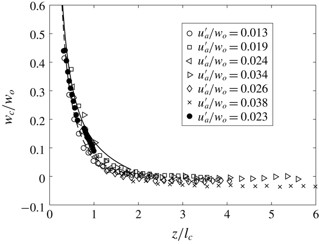
with experimental data of both this study and Khorsandi et al. (Reference Khorsandi, Gaskin and Mydlarski2013). It can be seen that the data generally collapsed on a single curve (lines are predictions from the integral model that will be discussed later), indicating that
 $l_{c}$
is a suitable length scale to normalize the downstream distance. When
 $z/l_{c}>2$
, it can be seen that the velocity has decayed to zero, implying that the jet has been broken up by the background turbulence. The dimensional analysis indicates that the velocity decay may also be dependent on the ratio
 $u_{a}^{\prime }/w_{o}$
. However, centreline velocity data of different ratios collapsed onto a single curve as in figure 10 suggesting that the dependence is weak before the jet is broken up. Thus the non-dimensional relationship becomes
 $$\begin{eqnarray}\displaystyle \unicode[STIX]{x1D719}^{\prime }\sim f\left(\frac{z}{l_{c}}\right). & & \displaystyle\end{eqnarray}$$
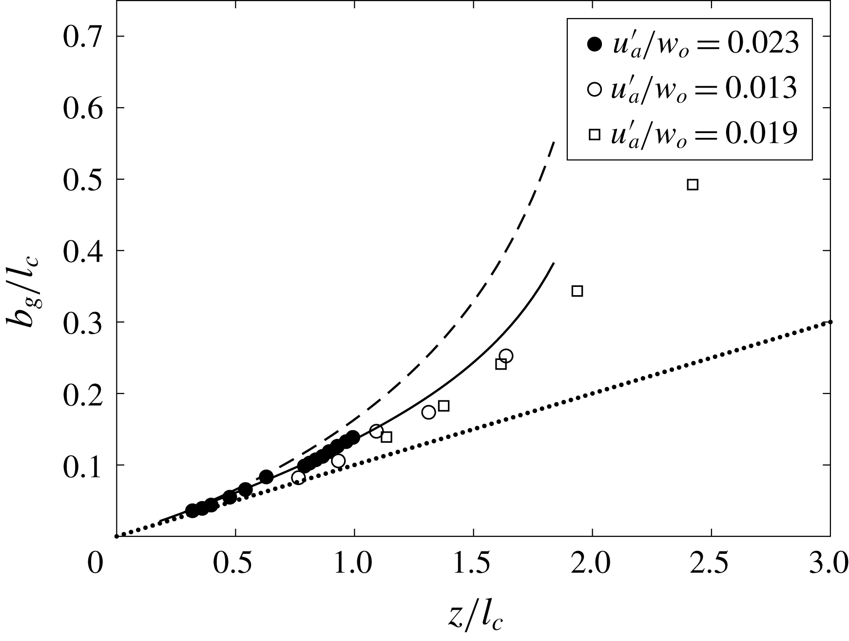
This is also evident in the Gaussian half-widths measured both in this study and that of Khorsandi et al. (Reference Khorsandi, Gaskin and Mydlarski2013) (figure 11), in which the data can be seen to collapse on a single curve when
 $l_{c}$
is used as the normalizing length scale. The growth of the jet is in general nonlinear, and the growth rate increases as
 $z/l_{c}$
increases. It is generally consistent with the observation of past studies that the spreading rate increases significantly when the background turbulence intensity reaches a threshold level (Ching et al.
Reference Ching, Fernando and Robles1995). However, the increase in spreading rate appears to be more gradual than what was observed in Law et al. (Reference Law, Cheng and Davidson2001), possibly due to the fact that the background turbulence generated in past studies was inhomogeneous, with a drastic increase in strength close to the downstream oscillating grid. By contrast, in this study and in that of Khorsandi et al. (Reference Khorsandi, Gaskin and Mydlarski2013), the turbulence was more homogeneous.
The normalized centreline velocity of a jet in background turbulence. Experimental data from Khorsandi et al. (Reference Khorsandi, Gaskin and Mydlarski2013) (open symbols) and this study (filled symbols). Solid and dashed lines are the integral model predictions based on the linear and exponential best-fit lines in representing the momentum decay, respectively.

The normalized Gaussian half-width of a jet in background turbulence. Experimental data from Khorsandi et al. (Reference Khorsandi, Gaskin and Mydlarski2013) (open symbols) and this study (filled symbols). Dotted line represents the spread of a jet in quiescent ambient. Solid and dashed lines are the integral model predictions based on the linear and exponential best-fit lines in representing the momentum decay, respectively.

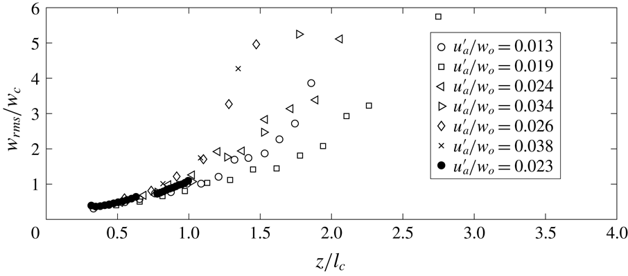
The centreline turbulence intensity of the axial velocity of a jet in turbulence is shown in figure 12. When
 $z/l_{c}$
is close to zero, it is expected that
 $w_{rms}/w_{o}$
will be similar to that of a jet in quiescent ambient (about 0.25), since the background turbulence effects have not come into play. As
 $z/l_{c}$
increases, the effect of the background turbulence also increases, and it can be seen from figure 12 that the turbulence intensity increases from about 0.25 to 1.0 when
 $z/l_{c}$
reaches 1. Within
 $z/l_{c}=0.25{-}1$
, the measurements collapse relatively well onto a single curve, and the dependence of
 $w_{rms}/w_{c}$
on
 $u_{a}^{\prime }/w_{o}$
is still not strong. When
 $z/l_{c}>1$
, the data begin to diverge, and in all cases the
 $w_{rms}$
level is greater than
 $w_{c}$
, showing the significance of the effect of background turbulence. When this occurs, it is an indication that the jet has started to be broken up by the background turbulence. Results also showed that when
 $z/l_{c}>1$
, the turbulence intensity of the axial velocity will be dependent on the ratio
 $u_{a}^{\prime }/w_{o}$
in addition to
 $z/l_{c}$
. When
 $u_{a}^{\prime }/w_{o}$
increases, the effects of the background turbulence can also be seen to increase, with
 $w_{rms}/w_{c}$
going as high as 5 when
 $z/l_{c}=2.0$
.
We now focus on the regime
 $z/l_{c}<\sim 1$
for model development, because the variation of
 $w_{rms}/w_{c}$
is more predictable. The ratio
 $w_{rms}/w_{c}$
generally increased nonlinearly from 0.25 at
 $z/l_{c}=0$
to 1.2 when
 $z/l_{c}=1$
regardless of the ratio
 $u_{a}^{\prime }/w_{o}$
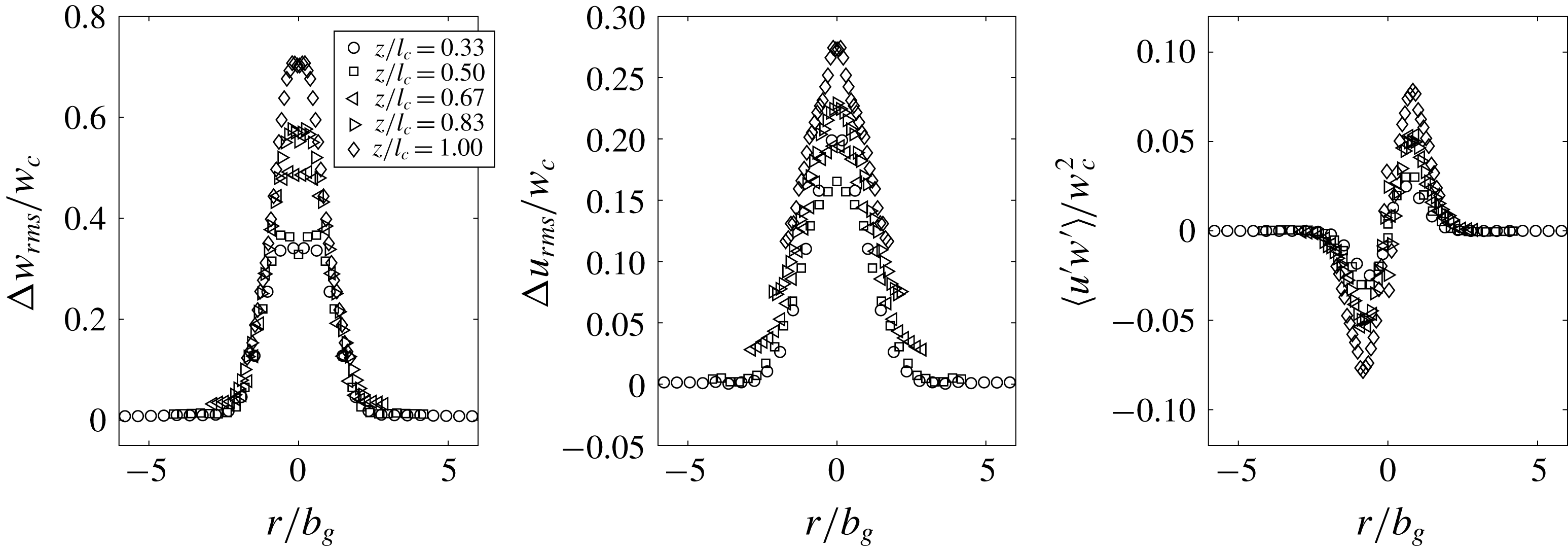
. The cross-sectional profiles of the second-order statistics at selected
 $z/l_{c}$
are given in figure 13. Note that the data are plotted symmetrically about
 $r=0$
as only one side of the data was measured to increase the field of view. The excess turbulence intensity of the axial velocity
 $\unicode[STIX]{x0394}w_{rms}=w_{rms}-u_{a}^{\prime }$
can be seen to increase monotonically from 0.25, like that of a jet in quiescent ambient, to about 0.7 at
 $z/l_{c}\approx 1$
. Interestingly, the effect of the background turbulence has caused the jet to become increasingly anisotropic; the excess turbulence intensity of the radial velocity
 $\unicode[STIX]{x0394}u_{rms}=u_{rms}-u_{a}^{\prime }$
has stayed in the range of 0.15–0.25, and increased less by the background turbulence. On the contrary, the shear stress inside the jet can be clearly seen to be enhanced by the background turbulence, but outside of the jet the shear stress is always zero, a property of the HIT. This would imply that momentum flux will be conserved even with the presence of background HIT as discussed in the next subsection.
The normalized centreline r.m.s. axial velocity of a jet in background turbulence. Experimental data from Khorsandi et al. (Reference Khorsandi, Gaskin and Mydlarski2013) (open symbols) and this study (filled symbols). At
 $z/l_{c}=0$
,
 $w_{rms}/w_{c}\approx 0.25$
(Wang & Law Reference Wang and Law2002).

Cross-sectional profiles of the second-order statistics of a jet in background turbulence (mirrored about
 $r=0$
). Solid lines represent the profiles for
 $u_{a}^{\prime }=0~\text{m}~\text{s}^{-1}$
(Wang & Law Reference Wang and Law2002).

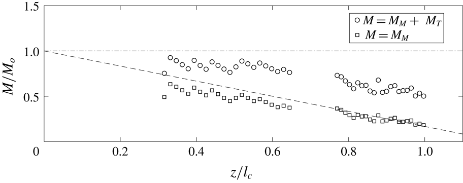
The variation of the momentum integral
 $M$
along
 $z$
with (circles) or without (squares) accounting for the second-order statistics measured in this study (
 $u_{a}^{\prime }/w_{o}=0.023$
).

4.2.1 Conservation of momentum
The momentum conservation principle of a jet in background turbulence was examined in Khorsandi et al. (Reference Khorsandi, Gaskin and Mydlarski2013). Different from a jet in quiescent ambient, the mean momentum integral
 $M_{M}=\int _{0}^{\infty }2\unicode[STIX]{x03C0}r\unicode[STIX]{x1D70C}u^{2}\,\text{d}r$
was found not to be constant but to decrease along
 $z$
. The finding is crucial to the development of the jet integral model when there is background turbulence. In § 2, we showed that while the mean momentum is not conserved as suggested in Khorsandi et al. (Reference Khorsandi, Gaskin and Mydlarski2013), the conservation of total momentum flux remains valid when the second-order statistics are included. Using the experimental data of this study, we re-examined the problem by including the second-order statistics of the jet in the momentum integral. The total momentum flux equation of a jet in background turbulence is given as
 $$\begin{eqnarray}\displaystyle M=\int _{0}^{\infty }2\unicode[STIX]{x03C0}(\overline{w}^{2}+\overline{w^{\prime 2}}-\overline{u^{\prime 2}})r\,\text{d}r. & & \displaystyle\end{eqnarray}$$
The integral is evaluated for
 $z/l_{c}=0.3{-}1.0$
using our data, and the results are plotted in figure 14. Without accounting for the second-order statistics, the momentum can be seen to decrease along
 $z$
, similar to that observed by Khorsandi et al. (Reference Khorsandi, Gaskin and Mydlarski2013). The jet has an initial momentum of
 $M_{o}$
, but decreases to about
 $0.2M_{o}$
when the jet reaches
 $z/l_{c}\approx 1$
. However, when the second-order statistics are included, the momentum flux is closer to
 $M_{o}$
for
 $z/l_{c}=0{-}1.0$
; it should be noted that a portion of the momentum flux might be out of the camera field of view for
 $z/l_{c}>0.6$
, where the shear stress is also non-zero, and this appears to have led to a drop in the momentum downstream. Overall, except for this experimental limitation, the total momentum flux can be seen to be conserved with downstream distance in the presence of background HIT.
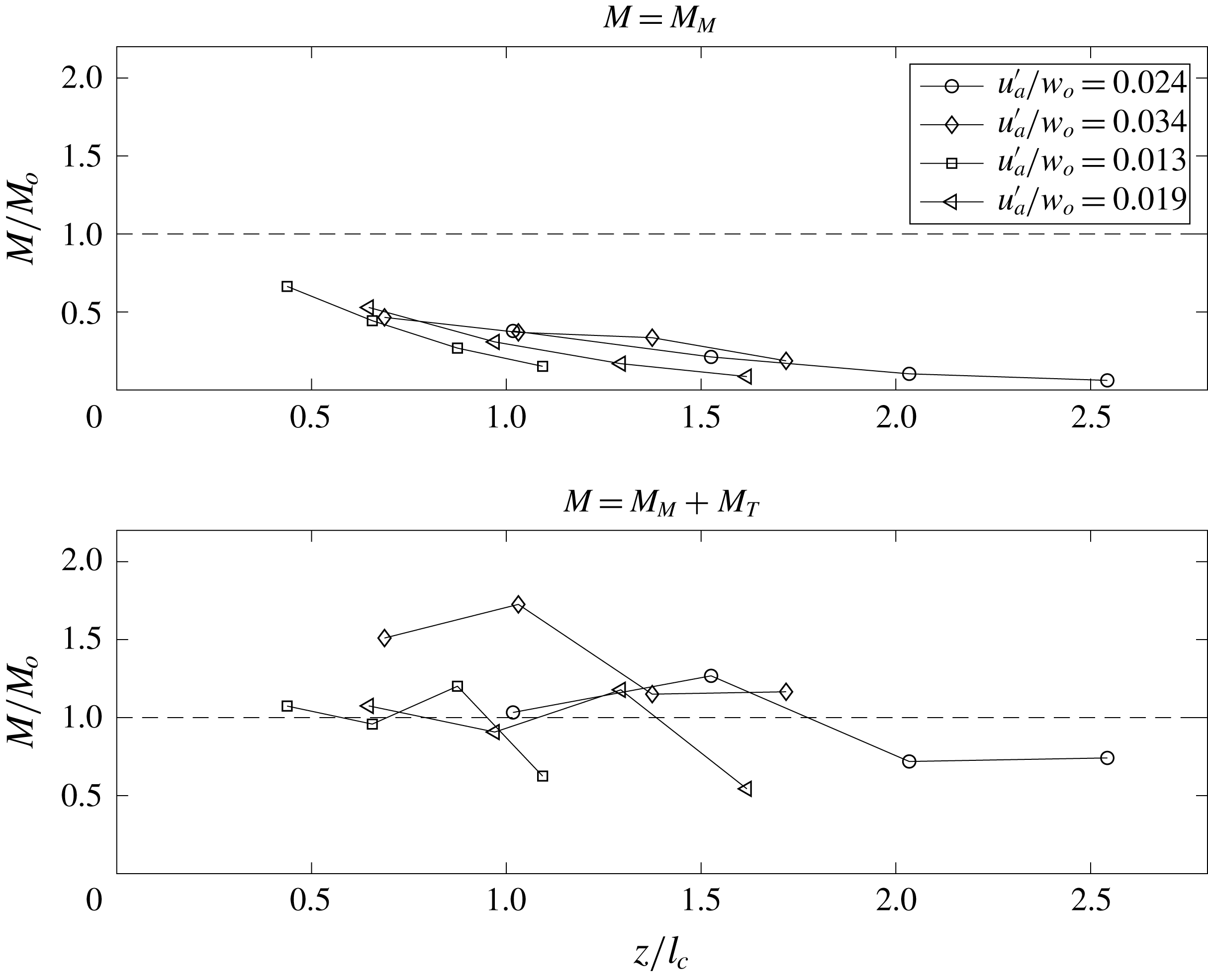
The cross-sectional velocity and r.m.s. axial velocity profile of Khorsandi et al. (Reference Khorsandi, Gaskin and Mydlarski2013) were extracted and used to re-examine the momentum flux conservation for a jet in background turbulence. It should be noted that the r.m.s. radial velocity profiles were not reported in their paper, but from our experimental data the contribution from radial r.m.s. velocity is typically
 $1/3$
of that contributed by the axial r.m.s. velocity, and this is assumed in the analysis of their data. In figure 15(a), the momentum flux integrals of a jet in background turbulence, with various
 $w_{o}/u_{a}^{\prime }$
ratios, were computed by only accounting for the mean flow. It can be seen that the momentum flux decayed along
 $z$
, and when the jet reached
 $z/l_{c}=1.5$
, the momentum flux dropped to only about 0.1 of that of the initial momentum flux. However, when the second-order statistics were accounted for in the integral, the total momentum flux downstream maintained relatively constant (figure 15
b). This suggests that the momentum flux can only be conserved when the second-order statistics are accounted for. In other words, the conservation of momentum should be up to second order for integral modelling in order to cater for a jet discharge in a background HIT.
The variation of momentum flux along
 $z$
of a jet in background turbulence with and without accounting for the second-order statistics (Khorsandi et al.
Reference Khorsandi, Gaskin and Mydlarski2013).

The variation of the momentum ratio downstream for a momentum jet in background turbulence for
 $z/l_{c}<2$
. Experimental data from Khorsandi et al. (Reference Khorsandi, Gaskin and Mydlarski2013) (open symbols) and this study (filled symbols). Solid and dashed lines are the linear and best-fit curve satisfying the boundary conditions
 $(z/l_{c},M_{M}/M)=(0,1)$
and
 $(z/l_{c},M_{M}/M)=(2,0)$
, respectively.

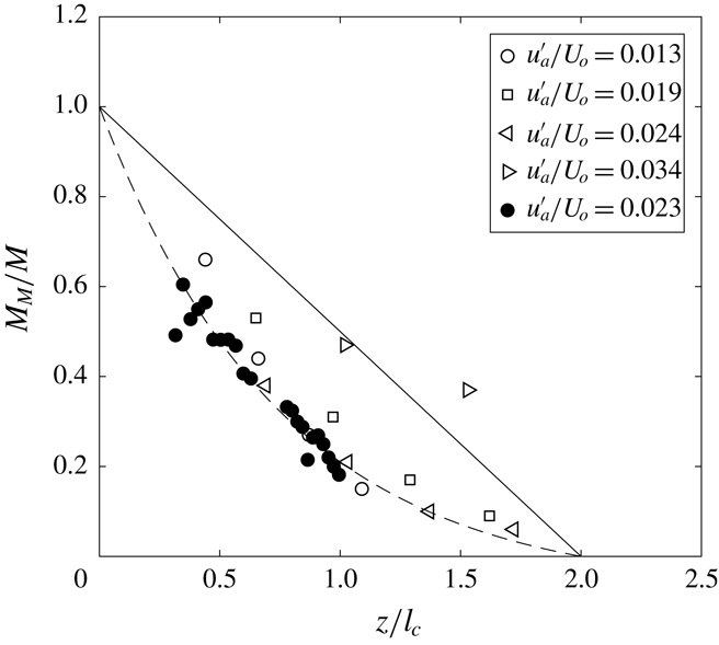
4.2.2 Predictions from integral model
For a jet in quiescent ambient, the ratio of jet momentum carried by the mean flow and the eddies remained approximately constant independent of the downstream distance as
 $k_{M}\approx 1.10$
(Wang & Law Reference Wang and Law2002). This also indicated that the momentum of the jet is mainly transported by the mean flow. For a jet in background turbulence, however, the percentage of jet momentum being transported by the eddies is increasing downstream, so that the value of
 $k_{M}$
keeps increasing. Figure 16 shows the change in momentum ratio with
 $z/l_{c}$
. It can be seen that most of the momentum is transported by the mean flow initially, but then the momentum becomes increasingly transported by the eddies, and the momentum ratio decreases. When
 $z/l_{c}$
reaches about 1.5, the momentum ratio falls to about 0.1, which indicates that most of the momentum is now transported by the eddies. The measurements of momentum ratio can be used to obtain the
 $k_{M}$
variation with
 $z/l_{c}$
. A line represented by the equation
 $$\begin{eqnarray}\displaystyle k_{M}=\frac{1}{-0.5(z/l_{c})+1}, & & \displaystyle\end{eqnarray}$$
which guarantees
 $M_{M}=M_{o}$
when
 $z=0$
, and
 $M_{M}=0$
when
 $z/l_{c}=2$
(an assumed linear decay), represents the trend of the experimental data well for
 $z/l_{c}<2$
, and can be adopted. It is noted that our data show a linear decay, while those from Khorsandi et al. (Reference Khorsandi, Gaskin and Mydlarski2013) appear to be exponential. An exponential fit which guarantees the same boundary conditions gives
 $$\begin{eqnarray}\displaystyle k_{M}=\frac{1}{1.076\exp [-0.1.324(z/l_{c})]-0.076}. & & \displaystyle\end{eqnarray}$$
By substituting equation (4.3) or (4.4) into the integral model outlined in § 2, the mixing characteristics of a jet in background turbulence can be predicted. Figure 10 shows the comparison of the predicted and observed centreline velocities. Solid and dashed lines are the linear and exponential best-fit curve satisfying the boundary conditions
 $(z/l_{c},M_{M}/M)=(0,1)$
and
 $(z/l_{c},M_{M}/M)=(2,0)$
, respectively. Predictions using both curves can be seen to be in good agreement with observation. Comparing to the case of a jet in quiescent ambient, the velocity decays much more rapidly to almost zero when
 $z/l_{c}\approx 1.5$
, i.e. the jet is now broken up by the background turbulence. Figure 11 shows the comparison between the predicted and observed spreading of a jet in background turbulence; again the predictions can be seen to be in good agreement with the experimental data for
 $z/l_{c}<1.5$
.
5 Buoyant jets in background turbulence
5.1 Mixing characteristics
For a buoyant jet in background turbulence, observations are generally similar to those of a pure jet in background turbulence. The buoyant jet can be seen to meander due to the large eddies, and smaller eddies change the jet structure. The
 $l_{c}$
in the buoyant jet experiments was chosen to be the same as that of a pure momentum jet for
 $1<z/l_{M}<5$
– which will eventually be justified by experimental data. As
 $l_{M}\sim f(Fr)$
, the non-dimensional relationship can be written as
 $$\begin{eqnarray}\displaystyle \unicode[STIX]{x1D719}^{\prime }\sim f\left(Fr,\frac{z}{l_{c}}\right). & & \displaystyle\end{eqnarray}$$
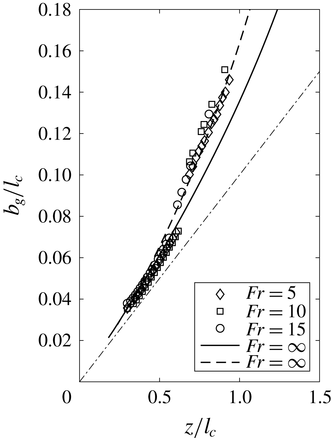
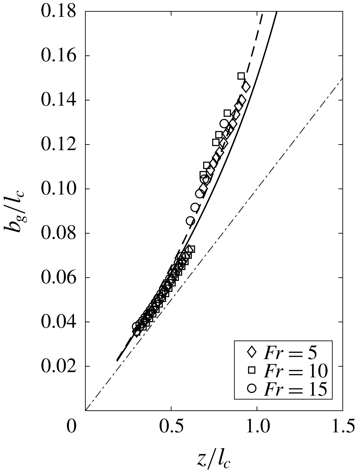
Figure 17 shows the spreading of the buoyant jet, with the length scales normalized by
 $l_{c}$
. It can be seen that the spreading rate has been significantly enhanced by the background turbulence, with the initial spreading rate increasing from about 0.10 for a quiescent buoyant jet to 0.18 when there was background turbulence. The growth rate increases even more downstream, when the background eddies have affected the jet more significantly. We note that the spread rate is not strongly dependent on
 $Fr$
for the range of
 $Fr$
studied, and is close to that observed in the pure jet discharge case.
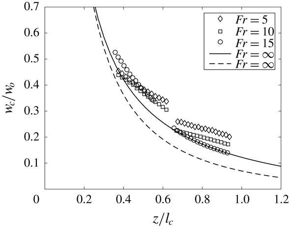
The centreline velocity of a buoyant jet in background turbulence is given in figure 18. A marked dependence on
 $Fr$
is observed in this case. The more buoyant the discharge is, the higher the velocity will be in general. Thus, it is difficult to use a single curve to represent the velocity decay for all
 $Fr$
. An integral model is needed in order to predict the mixing characteristics of the buoyant jet. The necessary quantities required for the model are
 $k_{M}$
and
 $k_{H}$
, which have to be obtained experimentally by measuring the second-order statistics of the buoyant jet in background HIT (see § 5.3).
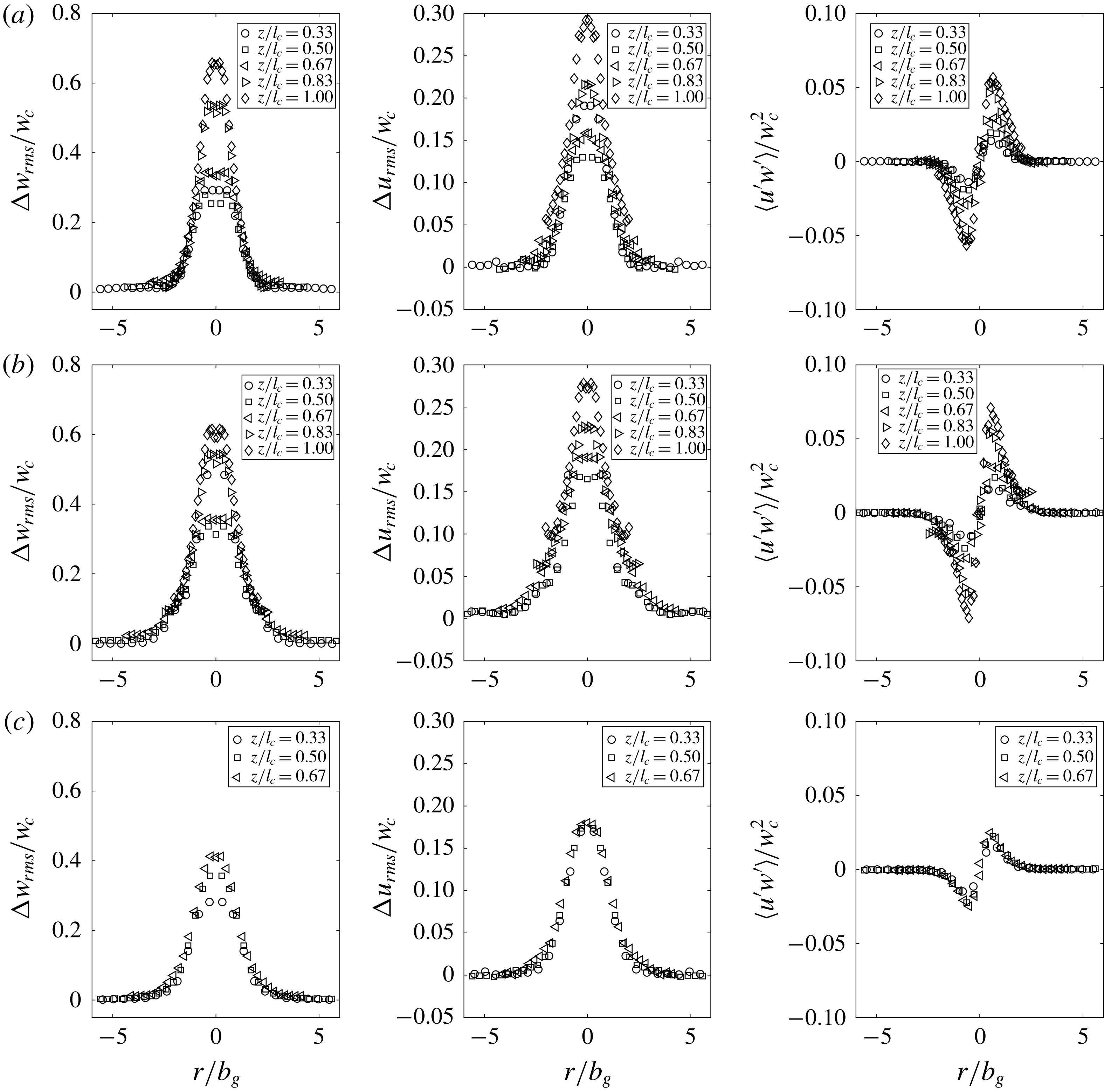
The second-order statistics of a buoyant jet in background turbulence are given in figure 19 with
 $Fr=5{-}15$
. For the turbulence intensity of the axial velocity, it can be seen that as the distance from the source increases, the turbulence intensity also increases. Similar to the case of a pure momentum jet, the peak turbulence intensity increases from about 0.25 to 0.70 when
 $z/l_{c}\approx 1$
. For the turbulence intensity of the radial velocity, the effect appears not as significant, with a modest increase of turbulence intensity from 0.18 to 0.30. For the shear stress, inside the jet the shear stress has increased noticeably from 0.015 to 0.070 at
 $z/l_{c}\approx 1$
, but outside of the jet it is zero and the momentum equation outlined in § 2 remains valid.
Spreading of a buoyant jet in background turbulence. Dash-dotted line represents the case
 $u_{a}^{\prime }=0$
predicted by the integral model. Solid and dashed lines are the predictions using linear and exponential best-fit curves for the momentum decay of a pure jet, respectively.

Centreline velocity of a buoyant jet in background turbulence. Solid and dashed lines are the predictions using linear and exponential best-fit curves for the momentum decay of a pure jet, respectively.

Second-order statistics of a buoyant jet in background turbulence: (a)
 $Fr=15$
; (b)
 $Fr=10$
; (c)
 $Fr=5$
.

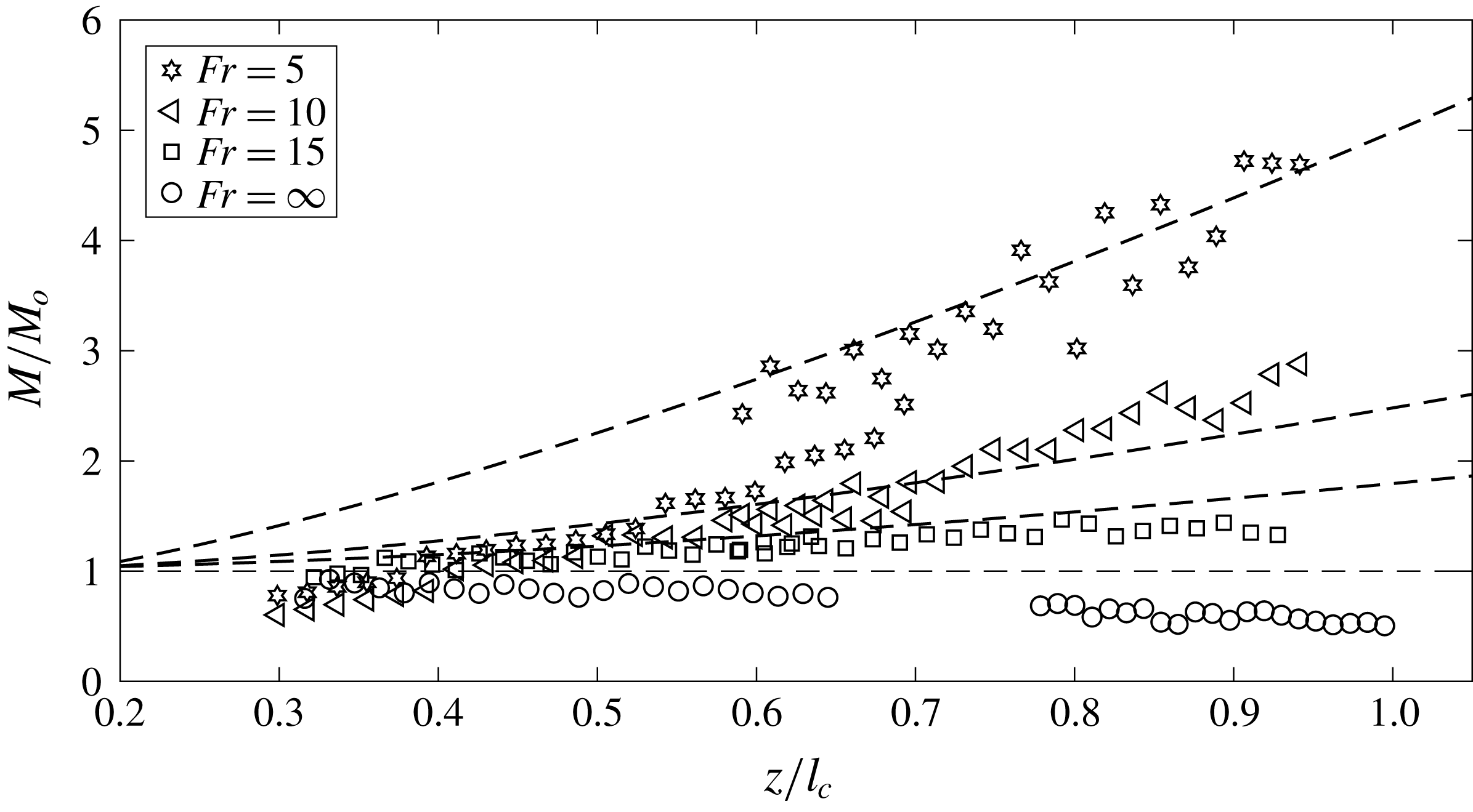
5.2 Conservation of momentum
For a buoyant jet, the momentum flux will be increased by the buoyancy of the jet. The total momentum flux equation has been given in § 2. To verify the equation, the change in total momentum with
 $z/l_{c}$
was obtained and is shown in figure 20. The lines represent the increase in the momentum flux of the jet due to its buoyancy, and can be obtained by solving an integral model of a buoyant jet in quiescent ambient. This is represented as
 $$\begin{eqnarray}\displaystyle 2\unicode[STIX]{x03C0}\int _{0}^{\infty }g\frac{\overline{\unicode[STIX]{x0394}\unicode[STIX]{x1D70C}}}{\unicode[STIX]{x1D70C}}r\,\text{d}r, & & \displaystyle\end{eqnarray}$$
which is the right-hand side of equation (2.5). The symbols in the figure represent the total momentum integral computed using the left-hand side of equation (2.5). It can be seen from the figure that the symbols are in reasonable agreement with the lines, showing that (2.5) is valid and can be used in the integral model development.
The variation of momentum of buoyant jets in background turbulence with normalized downstream distance. Dashed lines represent the estimated momentum increase due to the density difference between the jet and the ambient. From top to bottom:
 $Fr=5$
,
 $Fr=10$
,
 $Fr=15$
,
 $Fr=\infty$
.

5.3 Predictions from integral model
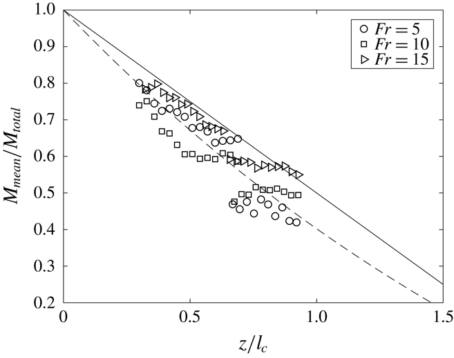
Similar to a jet in background turbulence, if the momentum ratio decay with
 $z/l_{c}$
is known, then the integral model presented in § 2 can be used to predict the mixing characteristics of a buoyant jet in background turbulence. Figure 21 shows the variation of momentum ratio with
 $z/l_{c}$
for a buoyant jet, from which
 $k_{M}$
can be determined. It can be seen that the variation of the momentum ratio of a buoyant jet can be well represented by the linear equation (4.3), in which the distance is normalized by the pure jet
 $l_{c}$
. Thus our experimental results suggest that
 $l_{c}$
defined by the jet initial momentum is also appropriate for buoyant jets with
 $1<z/l_{M}<5$
. Alternatively, the exponential best fit of the momentum decay which guarantees
 $M_{M}=M_{o}$
when
 $z=0$
and
 $M_{M}=0$
when
 $z/l_{c}=2$
can also be used in integral modelling:
 $$\begin{eqnarray}\displaystyle k_{M}=\frac{1}{1.828\exp [-0.396(z/l_{c})]-0.828}. & & \displaystyle\end{eqnarray}$$
An additional term required to be determined in the model is the ratio of the mean to total tracer mass or buoyancy flux along
 $z/l_{c}$
, equivalent to
 $1/k_{H}$
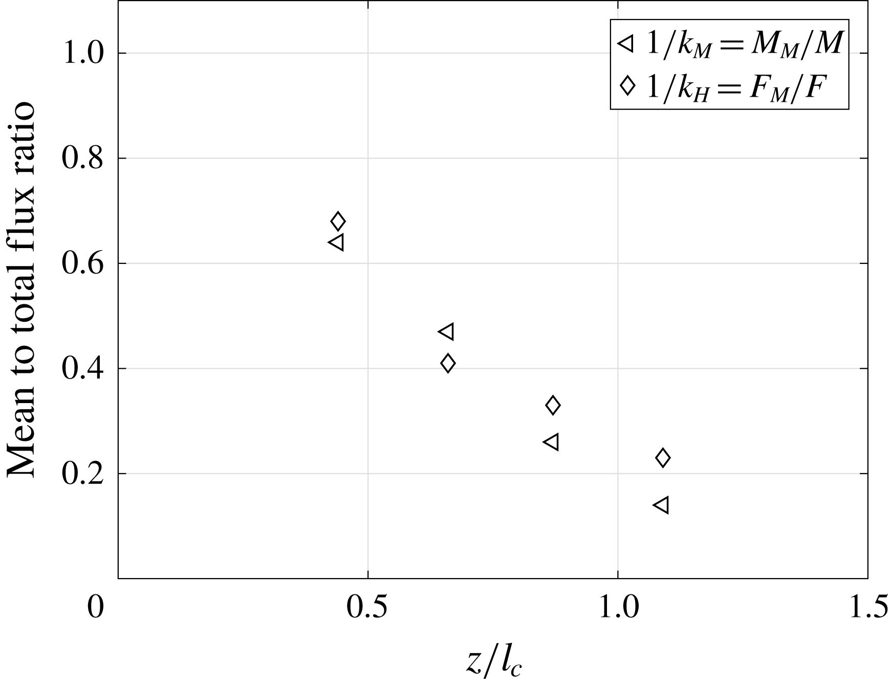
in equation (2.12). Although it is not measured directly in our experiments, Wang & Law (Reference Wang and Law2002) found that
 $k_{H}\approx k_{M}$
for both jets and plumes in quiescent ambient; the recent study of Perez-Alvarado (Reference Perez-Alvarado2016) also suggested that the evolution of mean tracer mass flux downstream is similar to that of the mean momentum flux for a jet in background HIT (figure 22), and hence it is reasonable to approximate
 $k_{H}=k_{M}$
for our modelling purpose.
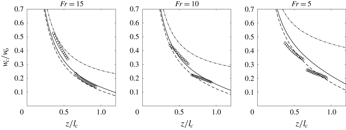
Figure 23 shows the comparison between the integral model predicted and observed centreline velocity of a buoyant jet in background turbulence. The solid or dashed lines represent the predictions with the background turbulence accounted for, while the dash-dotted lines represent the predictions in quiescent ambient. The predictions accounting for background turbulence are in good agreement with observations, while those without background turbulence can be seen to overestimate the velocity especially when buoyancy increases.
Figure 24 shows the comparison between predicted jet Gaussian half-width and observations. Most of the data collapse onto a single curve, suggesting that the dependence of Gaussian half-width on
 $Fr$
is weak for the range of
 $Fr$
studied. The solid and dashed lines are the prediction from the integral model of a buoyant jet in background turbulence using linear and exponential curve fits for the momentum decay, respectively, which show good agreement with the experimental data. In both prediction and observation, the growth rate of the jet Gaussian half-width increases from about 0.10 to 0.18. The growth of the jet can be seen to be nonlinear, and the growth rate increases as it goes downstream until the jet is broken up by the background turbulence.
The variation of the momentum ratio downstream for a buoyant jet in background turbulence. Solid and dashed lines are the linear and exponential best-fit curves for the momentum decay of buoyant jets satisfying the boundary conditions
 $(z/l_{c},M_{M}/M)=(0,1)$
and
 $(z/l_{c},M_{M}/M)=(2,0)$
, respectively.

The mean momentum and buoyancy flux decay of a jet in background HIT. Data from Perez-Alvarado (Reference Perez-Alvarado2016);
 $u_{a}^{\prime }/w_{o}=0.013$
.

Comparisons of the predictions (solid lines) of centreline velocity of a buoyant jet in background turbulence with observations (symbols). Dash-dotted lines are the predictions without accounting for the background turbulence. Solid and dashed lines are the predictions using linear and exponential best-fit curves for the momentum decay of buoyant jets, respectively.

Comparisons of model-predicted (solid line) jet width of a buoyant jet in background turbulence with observation. Dash-dotted line is the prediction without accounting for the background turbulence. Solid and dashed lines are the predictions using linear and exponential best-fit curves for the momentum decay of buoyant jets, respectively.

6 Discussion
6.1 Entrainment of a buoyant jet in background turbulence
Typical jet integral models associate an increase in jet spreading rate (for example when there is background turbulence) to an increase in entrainment. It is then natural to use a larger entrainment coefficient in the model to account for the effects of background turbulence on the jet. However, recent experiments of Khorsandi et al. (Reference Khorsandi, Gaskin and Mydlarski2013) showed that the entrainment into a jet will decrease instead in the presence of background turbulence, which is contrary to the physical expectation as discussed before. It is thus important to study whether the proposed model in this study can properly account for the decrease in entrainment based on the conservation of total momentum flux when there is background turbulence. We have carried out a test case and estimated the entrainment into the jet. The following discharge parameters are used:
 $D=0.01~\text{m}$
,
 $w_{o}=0.65~\text{m}~\text{s}^{-1}$
,
 $u_{a}^{\prime }=0.02~\text{m}~\text{s}^{-1}$
, integral length scale
 $L_{I}=0.1~\text{m}$
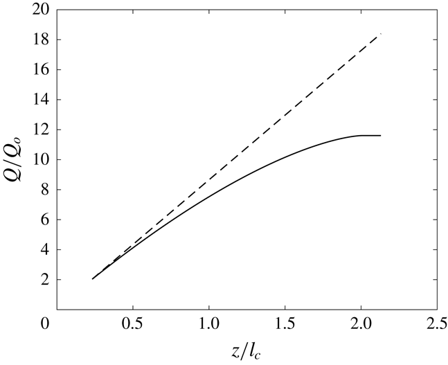
. In this simple case, it is assumed that there is no density difference between the source fluid and the ambient. The resulting predicted volume flux and thus entrainment by the model is shown in figure 25. With background turbulence, the entrainment can be seen to decrease significantly at about
 $z/l_{c}\approx 1$
compared to that without background turbulence, showing that the physics has been captured properly by the model. Effects of the background HIT on the entrainment coefficient are analysed preliminarily in appendix B, and the issue is suggested to be investigated in detail in the future.
The predicted volume flux (and thus entrainment) into a jet with (solid line) and without (dashed line) background turbulence.

6.2 The critical length scale
Dimensional analysis suggests that there can be two normalizing critical length scales for a buoyant jet – one defined by momentum
 $l_{cj}$
and the other by buoyancy
 $l_{cp}$
. While the choice of the length scale is clear for cases of a pure jet or a plume, experiments are eventually needed to determine which length scale is more appropriate for buoyant jet discharges. In our experiments, it was shown that
 $l_{cj}$
is an appropriate length scale for
 $1<z/l_{M}<5$
, as a single curve can be used to represent the momentum ratio variation with
 $z/l_{cj}$
. If
 $l_{cp}$
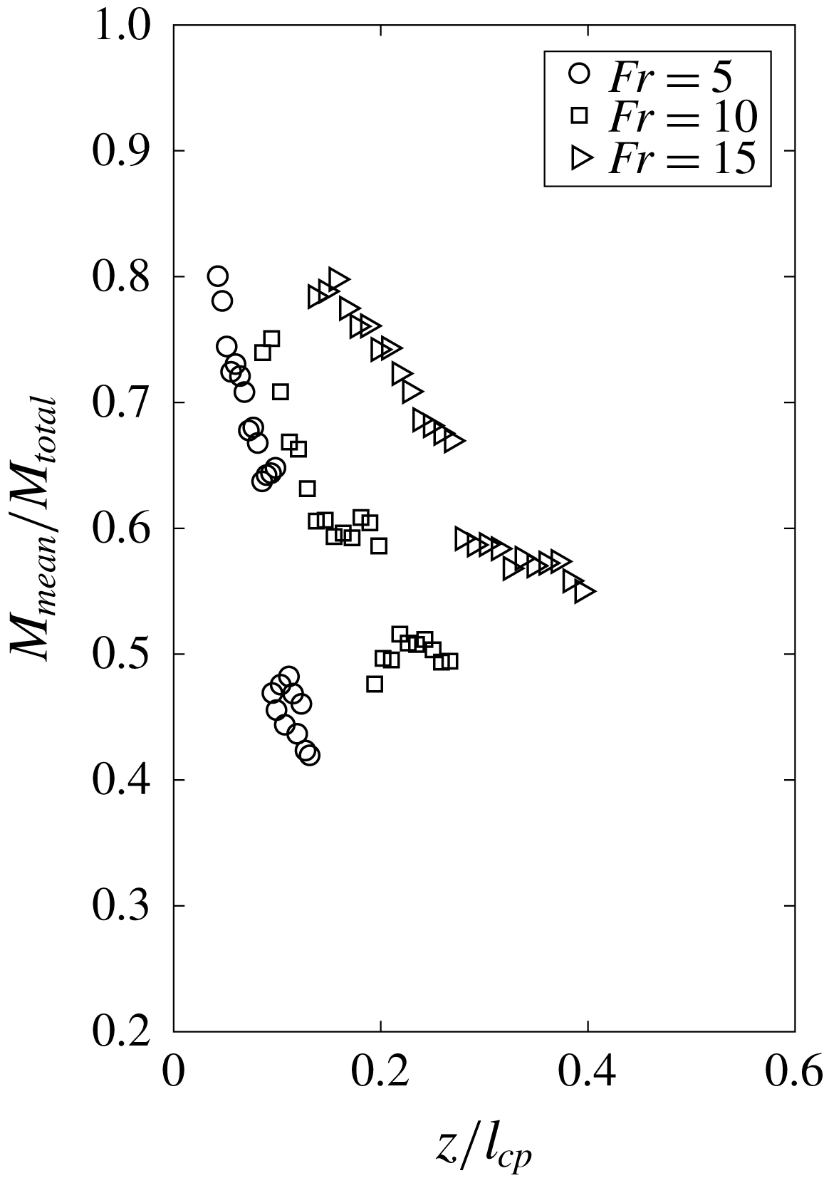
is used instead for the normalization, the resulting momentum variation is shown in figure 26. A dependence on
 $Fr$
can be observed which will complicate integral modelling. We note the recent study of Perez-Alvarado (Reference Perez-Alvarado2016), which showed the mean tracer mass flux (in this case density difference) to diminish quickly with
 $z/l_{cj}$
when there is background turbulence, may partly explain why the buoyancy effect is less important than expected in determining the critical length scale. It should be noted that the results are limited to
 $1<z/l_{M}<5$
, and hence when
 $z/l_{M}\gg 5$
, as can be seen in some applications, it is expected that
 $l_{cp}$
will be more appropriate. The issue of when
 $l_{cp}$
is more appropriate to be used should be further studied in the future.
The variation of the momentum ratio downstream for a buoyant jet in background turbulence using
 $l_{cp}$
for normalization.

6.3 Application of the model
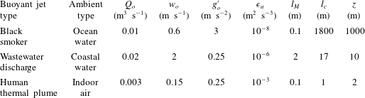
There are many applications that involve buoyant jets of different scales that discharge into a turbulent environment. Some examples and their typical discharge and ambient parameters, obtained from various sources, are shown in table 3. By estimating
 $l_{c}$
and the distance
 $z$
that is under consideration, one can quickly have a sense of the extent to which the jet will be affected by the background turbulence. It should be noted that for some cases where
 $z\gg l_{M}$
,
 $l_{c}$
is estimated based on the flow buoyancy. Black smokers from hydrothermal vents (Turner & Campbell Reference Turner and Campbell1987) typically originate from the ocean bed and are highly buoyant; the height of interest is typically
 ${\sim}$
1 km from the discharge point to the level at which the plume is trapped due to ambient density stratification. In this case
 $z/l_{c}\approx 0.5$
and the plume will not be broken up, although its spread rate and velocity will be somewhat affected. The same can be said for wastewater discharges in relatively shallow water in many Asian-Pacific coastal areas. In an indoor environment, where humans can generate thermal plumes (Linden Reference Linden1999), it can be expected that the background turbulence will have a stronger effect on the plume as the height of interest (say for example the ceiling height) is larger than
 $l_{c}$
. Even if the plume is not broken up by the turbulence, the entrainment will likely be affected. This could have some implications on the design of the height of ventilation windows (Linden, Lane-Serff & Smeed Reference Linden, Lane-Serff and Smeed1990).
Examples of buoyant jets with a background turbulence with typical discharge and ambient parameters. The dissipation rates for ocean and coastal waters were obtained from Petersen, Sanford & Kemp (Reference Petersen, Sanford and Kemp1998) and the geometric mean of the given magnitude range has been adopted. Data for an indoor environment were estimated from Loomans’ (Reference Loomans1998) measurement of eddy integral length and velocity scale. Typical discharge parameters for black smoker, wastewater and human thermal plume were obtained from Turner & Campbell (Reference Turner and Campbell1987), Lee & Chu (Reference Lee and Chu2003) and Craven & Settles (Reference Craven and Settles2006), respectively.

7 Conclusion
The effect of background HIT on buoyant jets has been investigated experimentally in this study. It has been observed that the large eddies of the turbulence cause a jet to meander, increasing the absolute spreading rate. The smaller eddies tend to interfere with the jet structure, modifying the second-order turbulence statistics of the jet. The mixing characteristics of the buoyant jet have been shown to vary with several dimensionless parameters. For a momentum jet, the mixing characteristics are mainly dependent on the critical length scale
 $l_{c}$
, which has been supported by experimental measurements of both the centreline velocity and jet Gaussian half-width from the present study, and that of Khorsandi et al. (Reference Khorsandi, Gaskin and Mydlarski2013). For a buoyant jet in background turbulence, which has not been reported previously, an additional parameter which governs the jet mixing is the densimetric Froude number
 $Fr$
.
 $Fr$
has been shown to influence centreline velocities for
 $Fr=5$
, 10 and 15, although its effect on other mixing characteristics, such as the second-order statistics, is less clear.
The governing equations for the integral modelling of a buoyant jet in background HIT have been derived. For a buoyant jet in quiescent ambient, the total momentum flux equation is mainly dominated by the mean flow term and the significance of second-order terms is less important in terms of the prediction of the jet mixing. However, for a buoyant jet in background HIT, we show that the second-order terms will become progressively more important as the background turbulence begins to affect the jet structure, and must be accounted for in an integral model. The decay of the mean momentum relative to the total momentum of a buoyant jet in background turbulence has been measured, and found to be mainly dependent on
 $l_{c}$
with a weaker dependence on
 $Fr$
for the range of
 $Fr$
studied, which can be well represented by the proposed linear equation or alternatively an exponential best-fit curve. An integral model has been proposed based on equations governing the total volume (using the entrainment assumption), total momentum and buoyancy fluxes of the buoyant jet, and also the mean momentum decay function along
 $z/l_{c}$
. The entrainment coefficient
 $\unicode[STIX]{x1D6FC}$
is affected by the background HIT generally which is not accounted for in our model, but preliminary analysis showed that accounting for the effects of HIT on
 $\unicode[STIX]{x1D6FC}$
causes relatively small changes in the predicted mixing characteristics of the buoyant jets in the region of interest of this study. Further detailed investigations are needed in the future to ascertain the effects of HIT on the entrainment coefficient of a buoyant jet. The model predictions are generally in good agreement with observations for both the jet Gaussian half-width which grows nonlinearly and the centreline velocity which decays noticeably faster than that without background HIT. The findings of this study can improve the predictions of buoyant jet mixing in a turbulent environment. Selected examples have been shown for illustration.
Acknowledgements
This research was supported by the National Research Foundation Singapore through the Singapore-MIT Alliance for Research and Technology’s Center for Environmental Sensing and Modeling interdisciplinary research programme. We thank Dr P. Liu for assistance in performing some of the experiments. The helpful comments and suggestions of the anonymous reviewers are gratefully acknowledged.
Appendix A. Control volume analysis of a buoyant jet in background HIT
The
 $z$
-momentum (2.2) can be derived using a CV approach. Consider the ring-shaped CV given in figure 1. With Boussinesq approximation, the net
 $z$
-momentum flux into the CV from the axial direction is
 $$\begin{eqnarray}\displaystyle (\unicode[STIX]{x0394}M_{z})_{a} & = & \displaystyle M_{out}-M_{in}\nonumber\\ \displaystyle & = & \displaystyle \left[\left(w+\frac{\unicode[STIX]{x2202}w}{\unicode[STIX]{x2202}z}\frac{\unicode[STIX]{x0394}z}{2}\right)^{2}-\left(w-\frac{\unicode[STIX]{x2202}w}{\unicode[STIX]{x2202}z}\frac{\unicode[STIX]{x0394}z}{2}\right)^{2}\right]2\unicode[STIX]{x03C0}\unicode[STIX]{x1D70C}r\unicode[STIX]{x2202}r\nonumber\\ \displaystyle & = & \displaystyle \left(2w\frac{\unicode[STIX]{x2202}w}{\unicode[STIX]{x2202}z}\unicode[STIX]{x0394}z\right)2\unicode[STIX]{x03C0}\unicode[STIX]{x1D70C}r\unicode[STIX]{x2202}r.\end{eqnarray}$$
The net
 $z$
-momentum flux into the CV from the lateral direction is (neglecting terms of
 $O(\unicode[STIX]{x0394}r^{3})$
)
 $$\begin{eqnarray}\displaystyle (\unicode[STIX]{x0394}M_{z})_{l} & = & \displaystyle M_{out}-M_{in}\nonumber\\ \displaystyle & = & \displaystyle \left[\left(u+\frac{\unicode[STIX]{x2202}u}{\unicode[STIX]{x2202}r}\frac{\unicode[STIX]{x0394}r}{2}\right)\left(w+\frac{\unicode[STIX]{x2202}w}{\unicode[STIX]{x2202}r}\frac{\unicode[STIX]{x0394}r}{2}\right)\left(r+\frac{\unicode[STIX]{x0394}r}{2}\right)\right.\nonumber\\ \displaystyle & & \displaystyle -\left.\left(u-\frac{\unicode[STIX]{x2202}u}{\unicode[STIX]{x2202}r}\frac{\unicode[STIX]{x0394}r}{2}\right)\left(w-\frac{\unicode[STIX]{x2202}w}{\unicode[STIX]{x2202}r}\frac{\unicode[STIX]{x0394}r}{2}\right)\left(r-\frac{\unicode[STIX]{x0394}r}{2}\right)\right]2\unicode[STIX]{x03C0}\unicode[STIX]{x1D70C}\unicode[STIX]{x2202}z\nonumber\\ \displaystyle & = & \displaystyle \frac{\unicode[STIX]{x2202}(ruw)}{\unicode[STIX]{x2202}r}(\unicode[STIX]{x0394}r)2\unicode[STIX]{x03C0}\unicode[STIX]{x1D70C}\unicode[STIX]{x2202}z.\end{eqnarray}$$
The pressure force acting on the CV in the
 $z$
-direction is given by
 $$\begin{eqnarray}\displaystyle F_{p} & = & \displaystyle F|_{z-\unicode[STIX]{x0394}z/2}-F|_{z+\unicode[STIX]{x0394}z/2}\nonumber\\ \displaystyle & = & \displaystyle \left[\left(P-\frac{\unicode[STIX]{x2202}P}{\unicode[STIX]{x2202}z}\frac{\unicode[STIX]{x0394}z}{2}\right)-\left(P+\frac{\unicode[STIX]{x2202}P}{\unicode[STIX]{x2202}z}\frac{\unicode[STIX]{x0394}z}{2}\right)\right]2\unicode[STIX]{x03C0}r\unicode[STIX]{x2202}r\nonumber\\ \displaystyle & = & \displaystyle -\frac{\unicode[STIX]{x2202}P}{\unicode[STIX]{x2202}z}2\unicode[STIX]{x03C0}r\unicode[STIX]{x2202}r\unicode[STIX]{x2202}z.\end{eqnarray}$$
The buoyancy force acting on the CV is given by
 $$\begin{eqnarray}\displaystyle F_{B}=\unicode[STIX]{x0394}\unicode[STIX]{x1D70C}gV=\unicode[STIX]{x0394}\unicode[STIX]{x1D70C}g(2\unicode[STIX]{x03C0}r\unicode[STIX]{x2202}r\unicode[STIX]{x2202}z). & & \displaystyle\end{eqnarray}$$
Since
 $F_{p}+F_{B}=(\unicode[STIX]{x0394}M_{z})_{a}+(\unicode[STIX]{x0394}M_{z})_{l}$
, we have
 $$\begin{eqnarray}\displaystyle \frac{\unicode[STIX]{x2202}w^{2}}{\unicode[STIX]{x2202}z}+\frac{1}{r}\frac{\unicode[STIX]{x2202}(ruw)}{\unicode[STIX]{x2202}r}=-\frac{1}{\unicode[STIX]{x1D70C}}\frac{\unicode[STIX]{x2202}P}{\unicode[STIX]{x2202}z}+\frac{\unicode[STIX]{x0394}\unicode[STIX]{x1D70C}}{\unicode[STIX]{x1D70C}}g. & & \displaystyle\end{eqnarray}$$
By Reynolds decomposition,
 $w=\overline{w}+w^{\prime }$
,
 $u=\overline{u}+u^{\prime }$
,
 $P=\overline{P}+P^{\prime }$
and
 $\unicode[STIX]{x1D70C}=\overline{\unicode[STIX]{x1D70C}}+\unicode[STIX]{x1D70C}^{\prime }$
. Substituting into (A 6), and time-averaging the equation, we have
 $$\begin{eqnarray}\displaystyle r\frac{\unicode[STIX]{x2202}(\overline{w^{2}}+\overline{w^{\prime 2}})}{\unicode[STIX]{x2202}z}+\frac{\unicode[STIX]{x2202}[r(\overline{u}~\overline{w}+\overline{u^{\prime }w^{\prime }})]}{\unicode[STIX]{x2202}r}=-\frac{r}{\overline{\unicode[STIX]{x1D70C}}}\frac{\unicode[STIX]{x2202}\overline{P}}{\unicode[STIX]{x2202}z}+r\frac{\overline{\unicode[STIX]{x0394}\unicode[STIX]{x1D70C}}}{\overline{\unicode[STIX]{x1D70C}}}g. & & \displaystyle\end{eqnarray}$$
Noting that the shear stress is identically zero in HIT (e.g. Pope Reference Pope2000) external to the jet and that
 $\overline{u^{\prime }w^{\prime }}$
is equal and opposite for positive and negative
 $\unicode[STIX]{x1D703}$
within the jet, the net contribution of the term to the
 $z$
-momentum balance is hence zero (note that this is not so for other types of turbulence). Integrating the remaining terms in the momentum balance equation along
 $r$
from 0 to
 $\infty$
, and noting that
 $(1/\unicode[STIX]{x1D70C})\unicode[STIX]{x2202}_{z}\overline{P}\approx -\unicode[STIX]{x2202}_{z}\overline{u^{\prime 2}}$
(e.g. Hussein et al.
Reference Hussein, Capp and George1994; Shabbir & George Reference Shabbir and George1994), will result in (2.5).
Appendix B. Entrainment coefficient of jets and plumes in background HIT
Generally the entrainment coefficient
 $\unicode[STIX]{x1D6FC}$
of a buoyant jet will be affected by the HIT since the Reynolds stresses are enhanced and the turbulence intensity profiles are changing downstream. The analytical formulation of
 $\unicode[STIX]{x1D6FC}$
derived by van Reeuwijk & Craske (Reference van Reeuwijkl and Craske2015), which relates
 $\unicode[STIX]{x1D6FC}$
directly to the first- and second-order turbulence statistics of a buoyant jet, enables us to make a preliminary assessment of the effect of HIT on
 $\unicode[STIX]{x1D6FC}$
based on our experimental results.
We adopt the definitions of van Reeuwijk & Craske (Reference van Reeuwijkl and Craske2015) for various buoyant jet fluxes in this appendix, with the mean volume flux
 $Q_{m}$
, momentum flux
 $M_{m}$
, buoyancy flux
 $F_{m}$
and integral buoyancy
 $B_{m}$
given as
 $$\begin{eqnarray}\displaystyle \left.\begin{array}{@{}c@{}}\displaystyle Q_{m}=2\int _{0}^{\infty }\overline{w}r\,\text{d}r,\quad M_{m}=2\int _{0}^{\infty }\overline{w}^{2}r\,\text{d}r,\quad B_{m}=2\int _{0}^{\infty }\overline{b}r\,\text{d}r,\\ \displaystyle F_{m}=2\int _{0}^{\infty }\overline{w}\overline{b}r\,\text{d}r=\frac{\unicode[STIX]{x1D703}_{m}M_{m}B_{m}}{Q_{m}}.\end{array}\right\} & & \displaystyle\end{eqnarray}$$
The definitions of various variables in the entrainment coefficient are given as (terms with subscript
 $g$
represent the sum of the terms with subscripts
 $m$
,
 $f$
and
 $p$
)
 $$\begin{eqnarray}\displaystyle \unicode[STIX]{x1D6FD}_{m}=\frac{M_{m}}{w_{m}^{2}r_{m}^{2}}=1,\quad \unicode[STIX]{x1D6FD}_{f}=\frac{2}{w_{m}^{2}r_{m}^{2}}\int _{0}^{\infty }\overline{w^{\prime 2}}r\,\text{d}r,\quad \unicode[STIX]{x1D6FD}_{p}=\frac{2}{w_{m}^{2}r_{m}^{2}}\int _{0}^{\infty }\overline{p}r\,\text{d}r, & & \displaystyle\end{eqnarray}$$
 $$\begin{eqnarray}\displaystyle \unicode[STIX]{x1D6FE}_{m}=\frac{2}{w_{m}^{3}r_{m}^{2}}\int _{0}^{\infty }\overline{w^{3}}r\,\text{d}r,\quad \unicode[STIX]{x1D6FE}_{f}=\frac{4}{w_{m}^{3}r_{m}^{2}}\int _{0}^{\infty }\overline{w}\overline{w^{\prime 2}}r\,\text{d}r,\quad \unicode[STIX]{x1D6FE}_{p}=\frac{4}{w_{m}^{3}r_{m}^{2}}\int _{0}^{\infty }\overline{w}\overline{p}r\,\text{d}r,\qquad \quad & & \displaystyle\end{eqnarray}$$
 $$\begin{eqnarray}\displaystyle \unicode[STIX]{x1D6FF}_{m}=\frac{4}{w_{m}^{3}r_{m}}\int _{0}^{\infty }\overline{w^{\prime }u^{\prime }}\frac{\text{d}\overline{w}}{\text{d}r}r\,\text{d}r,\quad \unicode[STIX]{x1D6FF}_{f}=\frac{4}{w_{m}^{3}r_{m}}\int _{0}^{\infty }\overline{w^{\prime 2}}\frac{\text{d}\overline{w}}{\text{d}z}r\,\text{d}r,\quad \unicode[STIX]{x1D6FF}_{p}=\frac{4}{w_{m}^{3}r_{m}}\int _{0}^{\infty }\overline{p}\frac{\text{d}\overline{w}}{\text{d}z}r\,\text{d}r, & & \displaystyle \nonumber\\ \displaystyle & & \displaystyle\end{eqnarray}$$
 $$\begin{eqnarray}\displaystyle \unicode[STIX]{x1D703}_{m}=\frac{F_{m}}{w_{m}b_{m}r_{m}^{2}},\quad \unicode[STIX]{x1D703}_{f}=\frac{2}{w_{m}b_{m}r_{m}^{2}}\int _{0}^{\infty }\overline{w^{\prime }b^{\prime }}r\,\text{d}r. & & \displaystyle\end{eqnarray}$$
The entrainment coefficient
 $\unicode[STIX]{x1D6FC}$
can generally be expressed as (van Reeuwijk & Craske Reference van Reeuwijkl and Craske2015; Craske & van Reeuwijk Reference Craske and van Reeuwijkl2016)
 $$\begin{eqnarray}\displaystyle \unicode[STIX]{x1D6FC} & = & \displaystyle \unicode[STIX]{x1D6FC}_{prod}+\unicode[STIX]{x1D6FC}_{disp}+\unicode[STIX]{x1D6FC}_{turb}+\unicode[STIX]{x1D6FC}_{buoy}\nonumber\\ \displaystyle & = & \displaystyle -\frac{\unicode[STIX]{x1D6FF}_{g}}{2\unicode[STIX]{x1D6FE}_{g}}+\frac{Q_{m}}{2\unicode[STIX]{x1D6FE}_{g}M_{m}^{5/2}}\frac{\unicode[STIX]{x2202}}{\unicode[STIX]{x2202}z}[(\unicode[STIX]{x1D6FE}_{g}-2\unicode[STIX]{x1D6FD}_{g}+1)M_{m}^{2}]+\frac{Q_{m}}{\unicode[STIX]{x1D6FE}_{g}M_{m}^{3/2}}(\unicode[STIX]{x1D6FD}_{g}-1)\frac{\unicode[STIX]{x2202}M_{m}}{\unicode[STIX]{x2202}z}+\left(\frac{1}{\unicode[STIX]{x1D6FD}_{g}}-\frac{\unicode[STIX]{x1D703}_{m}}{\unicode[STIX]{x1D6FE}_{g}}\right)Ri,\nonumber\\ \displaystyle & & \displaystyle\end{eqnarray}$$
where the first, second, third and fourth terms are the contributions from the TKE production, the dispersive effect, the turbulence intensity and the buoyancy effects, respectively (Craske & van Reeuwijk Reference Craske and van Reeuwijkl2015). We first consider the pure jet case, with
 $\unicode[STIX]{x1D6FC}_{buoy}=0$
. When there is no background HIT, the second and third terms vanish since the mean momentum flux of the jet remains constant along
 $z$
. When there is background HIT,
 $\text{d}M_{m}/\text{d}z$
is negative but it is not trivial to assess whether the two terms will contribute positively or negatively to
 $\unicode[STIX]{x1D6FC}$
. To better assess the effect of a background turbulence on
 $\unicode[STIX]{x1D6FC}$
, we first note that from our experimental results the turbulence statistics profiles of a jet in background HIT can be approximated by multiplying the corresponding profiles in quiescent background (e.g. the best-fit curves from Wang & Law (Reference Wang and Law2002)) by an increasing factor downstream, and the momentum decay can be approximated as
 $M_{m}=M(1-C_{M}z/l_{c})$
. Then we keep the assumption of
 $(1/\unicode[STIX]{x1D70C})\unicode[STIX]{x2202}_{z}\overline{P}\approx -\unicode[STIX]{x2202}_{z}\overline{u^{\prime 2}}$
, and it can be shown that
 $\unicode[STIX]{x1D6FD}_{g}$
,
 $\unicode[STIX]{x1D6FE}_{g}$
and
 $\unicode[STIX]{x1D6FF}_{g}$
for
 $0<z/l_{c}<1$
can be approximated as
 $$\begin{eqnarray}\displaystyle & \displaystyle \unicode[STIX]{x1D6FD}_{g}=1+C_{\unicode[STIX]{x1D6FD}}(z/l_{c}), & \displaystyle\end{eqnarray}$$
 $$\begin{eqnarray}\displaystyle & \displaystyle \unicode[STIX]{x1D6FE}_{g}=\unicode[STIX]{x1D6FE}_{m0}+(1+C_{\unicode[STIX]{x1D6FE}_{f}}z/l_{c})\unicode[STIX]{x1D6FE}_{f0}+\unicode[STIX]{x1D6FE}_{p0}, & \displaystyle\end{eqnarray}$$
 $$\begin{eqnarray}\displaystyle & \displaystyle \unicode[STIX]{x1D6FF}_{g}=(1+C_{\unicode[STIX]{x1D6FF}_{m}}z/l_{c})\unicode[STIX]{x1D6FF}_{m0}+(1+C_{\unicode[STIX]{x1D6FF}_{f}}z/l_{c})\unicode[STIX]{x1D6FF}_{f0}+\unicode[STIX]{x1D6FF}_{p0}, & \displaystyle\end{eqnarray}$$
where subscript
 $0$
represents the value of the variables in quiescent background. The change in the subscript
 $p$
terms relative to that in quiescent background is small since
 $(1/\unicode[STIX]{x1D70C})\unicode[STIX]{x2202}_{z}\overline{P}\approx -\unicode[STIX]{x2202}_{z}\overline{u^{\prime 2}}$
and the profile of
 $\overline{u^{\prime 2}}$
is not changed significantly based on our experimental results for a buoyant jet in HIT. Expanding the expression of
 $\unicode[STIX]{x1D6FC}$
, we have
 $$\begin{eqnarray}\displaystyle & \displaystyle \unicode[STIX]{x1D6FC}_{prod}=-\frac{\unicode[STIX]{x1D6FF}_{g}}{2\unicode[STIX]{x1D6FE}_{g}}, & \displaystyle\end{eqnarray}$$
 $$\begin{eqnarray}\displaystyle & \displaystyle \unicode[STIX]{x1D6FC}_{disp}=-\frac{C_{M}}{\unicode[STIX]{x1D6FE}_{g}}\frac{r_{m}}{l_{c}}\frac{\unicode[STIX]{x1D6FE}_{g}+1-2\unicode[STIX]{x1D6FD}_{g}}{1-C_{M}(z/l_{c})}+\frac{1}{2\unicode[STIX]{x1D6FE}_{g}}\frac{r_{m}}{l_{c}}(\unicode[STIX]{x1D6FE}_{f0}C_{\unicode[STIX]{x1D6FE}_{f}}-2C_{\unicode[STIX]{x1D6FD}}), & \displaystyle\end{eqnarray}$$
 $$\begin{eqnarray}\displaystyle & \displaystyle \unicode[STIX]{x1D6FC}_{turb}=-\frac{C_{M}}{\unicode[STIX]{x1D6FE}_{g}}\frac{r_{m}}{l_{c}}\frac{\unicode[STIX]{x1D6FD}_{g}-1}{1-C_{M}(z/l_{c})}. & \displaystyle\end{eqnarray}$$
We tabulate the values of different variables used in our analysis in table 4, which were averaged values from the direct numerical simulation studies of Craske & van Reeuwijk (Reference Craske and van Reeuwijkl2015, Reference Craske and van Reeuwijkl2016). Further, from our experimental data,
 $C_{M}\approx 0.5$
,
 $C_{\unicode[STIX]{x1D6FF}_{f}}\approx 1$
,
 $C_{\unicode[STIX]{x1D6FF}_{m}}\approx 2$
,
 $C_{\unicode[STIX]{x1D6FE}_{f}}\approx 1$
and
 $C_{\unicode[STIX]{x1D6FD}}\approx 0.75$
. Substituting these into the expanded entrainment coefficient formula,
 $\unicode[STIX]{x1D6FC}$
can be expressed as a function of
 $z/l_{c}$
. The variation of
 $\unicode[STIX]{x1D6FC}$
with
 $z/l_{c}$
for a jet is given in figure 27. The
 $\unicode[STIX]{x1D6FC}$
for a plume can be obtained by adding the buoyancy effects
 $\unicode[STIX]{x1D6FC}_{buoy}=(1/\unicode[STIX]{x1D6FD}_{g}-\unicode[STIX]{x1D703}_{m}/\unicode[STIX]{x1D6FE}_{g})Ri$
to
 $\unicode[STIX]{x1D6FC}$
. Noting that
 $\unicode[STIX]{x1D703}_{m}\approx 1$
and
 $Ri\approx 0.19$
for a plume, the variation of
 $\unicode[STIX]{x1D6FC}$
with
 $z/l_{c}$
for a plume is given in figure 28. Note that all
 $\unicode[STIX]{x1D6FC}$
have been converted from the definitions of van Reeuwijk & Craske (Reference van Reeuwijkl and Craske2015) to those that are traditionally used in the figures (
 $\unicode[STIX]{x1D6FC}=0.057$
for jets and
 $\unicode[STIX]{x1D6FC}=0.086$
for plumes).
From the two figures, it can be seen that the background turbulence increases the TKE production term
 $\unicode[STIX]{x1D6FC}_{prod}$
due to the increased Reynolds stresses. For both jets and plumes, the increment of
 $\unicode[STIX]{x1D6FC}_{prod}$
is about three times at
 $z/l_{c}=1$
. However, the dispersive and the turbulence intensity terms, which are associated with the momentum gradient
 $(\text{d}M_{m}/\text{d}z)$
, contributes negatively to
 $\unicode[STIX]{x1D6FC}$
up to about
 $z/l_{c}=0.8$
; the resulting decrease in
 $\unicode[STIX]{x1D6FC}$
is approximately equal to the increase due to the TKE production. The effects of the deceleration of the flow by the background HIT appear to have counteracted the effects of TKE production on
 $\unicode[STIX]{x1D6FC}$
. Overall, the change in
 $\unicode[STIX]{x1D6FC}$
is at most 20 % compared to that in quiescent ambient up to
 $z/l_{c}=0.8$
, which did not produce significantly different predictions. For
 $z/l_{c}>1.0$
, the increase in
 $\unicode[STIX]{x1D6FC}$
is more apparent close to the breakup point, but does not cause changes in jet mixing characteristics that are larger than the observed experimental variation (see figure 29). The more important factor is to be able to account for the decrease in jet mean momentum flux due to the background turbulence.
We emphasize that in the above analysis, a simple approach of using the Wang & Law (Reference Wang and Law2002) curve fits of various turbulence statistics profiles multiplied by a multiplication factor (determined by our experiments) has been used. More detailed investigations are needed to ascertain some observations that are counterintuitive. For example, it is possible for the term associated with the buoyancy to become negative when the mean to total TKE ratio decays faster than the momentum ratio (e.g. when
 $z/l_{c}>1$
in the plume
 $\unicode[STIX]{x1D6FC}$
plot), but this is speculative rather than conclusive. We opt to use
 $\unicode[STIX]{x1D6FC}$
for a quiescent background for the present modelling purpose until a devoted study on the entrainment coefficient of a buoyant jet in background turbulence has been established.
Entrainment coefficient of a jet in background HIT. Thin dotted line is the value of
 $\unicode[STIX]{x1D6FC}=0.057$
of a jet in quiescent background.

Entrainment coefficient of a plume in background HIT. Thin dotted line is the value of
 $\unicode[STIX]{x1D6FC}=0.086$
of a plume in quiescent background.

Comparison of the centreline velocity decay of a jet and a plume in background HIT predicted using
 $\unicode[STIX]{x1D6FC}$
of a quiescent background and that with the effects of HIT accounted for. The discharge parameters of the jet and plume
 $(Fr=5)$
are the same as those reported in the experiments of this paper.

Values of the parameters used in our entrainment coefficient analysis determined by the direct numerical simulation studies of Craske & van Reeuwijk (Reference Craske and van Reeuwijkl2015, Reference Craske and van Reeuwijkl2016).

Appendix C. Critical length scale of jets and plumes in background HIT
The critical length scale of a plume in background HIT,
 $l_{cp}$
, can be derived from physical arguments (Hunt Reference Hunt, Davies and Valente Neves1994). Following Hunt (Reference Hunt, Davies and Valente Neves1994), only the smaller scales of the background turbulence can affect the jet; larger eddies can only meander the jet without affecting its structure. Define
 $u^{\prime }<u_{a}^{\prime }$
(
 $u_{a}^{\prime }$
is the background r.m.s. velocity) as the velocity scale of the background turbulence with length scale/eddy size
 $L$
close to that of the plume
 $L\sim L_{P}<L_{I}$
, where
 $L_{P}$
is the plume characteristic length scale. When
 $u^{\prime }\sim u_{P}$
, the plume structure will be severely affected, where
 $u_{P}\sim F^{1/3}z^{-1/3}$
is the plume characteristic velocity, and
 $u^{\prime }$
can then be estimated as
 $u^{\prime }\sim (L\unicode[STIX]{x1D716}_{a})^{1/3}\sim (L_{P}\unicode[STIX]{x1D716}_{a})^{1/3}\sim (\unicode[STIX]{x1D6FD}z\unicode[STIX]{x1D716}_{a})^{1/3}$
, where
 $\unicode[STIX]{x1D6FD}$
is the jet spread rate. Hence when
 $u^{\prime }\sim u_{P}$
,
 $z=l_{cp}\sim (F/\unicode[STIX]{x1D716}_{a})^{1/2}$
.
The same argument also applies for a jet in background HIT. The characteristic velocity scale of the jet is
 $u_{J}\sim M_{1/2}z^{-1}$
, and when
 $u^{\prime }\sim (L\unicode[STIX]{x1D716}_{a})^{1/3}\sim (L_{J}\unicode[STIX]{x1D716}_{a})^{1/3}\sim (\unicode[STIX]{x1D6FD}z\unicode[STIX]{x1D716}_{a})^{1/3}\sim u_{J}$
, we have
 $z=l_{cj}\sim (M^{3}/\unicode[STIX]{x1D716}_{a}^{2})^{1/8}$
.