2.1. Generalities on supervised learning

Data-driven risk costing is a straightforward example of a statistical learning (a.k.a. machine learning) problem. Specifically, it is an example of supervised learning. We will see that statistical learning has a very rigorous way of building models based on data, parametrising them and validating them. Also, it has developed many different techniques for building models, some of which are little known to the actuarial community.

The term “learning” comes from the fact that we are trying to learn Footnote 1 the features of a model (structure and parameters) based on a sample of inputs and outputs, e.g. in rating factor selection the outputs are the claims and the inputs are the candidate rating factors. The term “supervised” reflects the fact that we know a number of actual outputs (e.g. the actual claims), and these drive our choice of the model. For this reason, supervised learning is also called “learning with a teacher”: during the training stage, the teacher feeds the model with pairs of inputs and outputs, and then selects a model. During the testing stage, the model is checked against new pairs of inputs and outputs.

A more mathematical definition, based on the discussion of statistical decision theory in Hastie et al. (Reference Hastie, Tibshirani and Friedman2001) (Section 2.4), is given below. According to this definition, supervised learning is a problem of functional optimisation.

Supervised learningGiven: (i) a real valued random input vector , (ii) a real valued output vector with joint distribution Pr(X,Y), (iii) a loss function L(Y, f(X)), that maps pairs (Y, f(X)) into positive real numbers, find Y = f(X) that minimises the expected prediction error EPE(f) = E(L(Y, f(X))).

This definition is helpful but loose: for example, it does not say to which class of function f must belong. In many cases, a countable dictionary of basis functions {f_α}_α∈N (the “basis functions”) will be specified, and f will be required to be written as a linear combination of these basis functions: f(x ₁, x ₂,…x_n) = ∑_α a_α f_α(x ₁, x ₂,… x_n), with ∑_α∣a_α∣²<∞. However, other possibilities exist, as we will see later.

As mentioned above, supervised learning is a two-stage process: (i) a training stage during which a model is fitted to the training data, i.e. a sample of pairs , and (ii) a testing phase, during which the model's goodness-of-fit is assessed against an independent subset of the data available.

One key issue is, as expected, the choice of the loss function. The most popular loss function for regression is the squared loss , where the functional is the L ₂ -norm, defined as for continuous functions and reducing to for discrete functions. Examples of alternative choices are the l ₁ norm, the l _∞ norm, the log P norm, etc.

2.2. Model selection

When selecting a model to interpret historical data, our main objective is to find one which has good (possibly optimal) predictive accuracy when presented with new independent data. It turns out that prediction accuracy is somehow related to the model complexityFootnote 2.

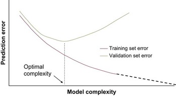
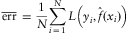
This relationship is illustrated in Figure 1, which shows the expected prediction error on both the training set (training error) and a test set (test error). The training error:

(1)

Figure 1

This graph illustrates a general behaviour of learning algorithms: the more complex the model becomes, the lower the training set error (red line). As for the validation set error (green line), it first decreases with complexity, and then picks up again. Model selection aims at striking the right balance – finding the optimal complexity (the minimum in the graph above).

always decreases as the model becomes more complex, as the model adapts to the nuances of the historical data. However, the test error:

(2)

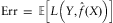
is large when the complexity is low (when the model is too simple to capture the regularities of the data), then decreases, and then picks up again (when the model starts overfitting the data). There is a point where the expected prediction error is minimal – the optimal complexity. The idea is that our model will have predictive power if it identifies the genuine regularities in the data, without adding any spurious features.

2.3. Model validation

The expected prediction error also guides the process of validating the model. With Solvency II approaching, validation has become a topical issue in insurance. The reader is referred for example to the report of the working party on model validation and monitoring presented at GIRO 2009 by Berry et al. (Reference Berry, Hemming, Matov and Morris2009) for a review.

The reason why the problem of model validation is so topical is that actuaries are subject, in their daily practice, to the pitfalls of data snooping. Data snooping (a.k.a. data dredging, or data fishing) is what happens when a data set is used to discover regularities, and the same data set is used to test the statistical significance of these regularities. This is a particularly important concern in disciplines where one makes intensive use of data mining (data mining will be mentioned more extensively in Section 3), e.g in medical research (see for example the papers White, Reference White2000 and by Ioannidis, Reference Ioannidis2005).

That this is a common problem in actuarial practice may be realised by the simple example of determining the severity distribution that fits a number of losses. If this is done without a clear hypothesis to test (e.g., that the severity distribution be a lognormal) one ends up choosing that severity distribution among those on offer in a distribution-fitting tool which happens to conform to the data in the closest fashion, perhaps because it has the lowest Kolmogorov-Smirnov distance (or any other statistical criterion). However, this closeness has typically no predictive value on future losses, since by choosing among, say, 20 distributions, some of which have 3 or 4 parameters, we are almost always bound to find a good fit by sheer chance. In other words, we have discovered regularities that are not really there.

Statistical learning provides the ideal framework to deal with data snooping as rigorously as possible, in that it provides clear protocols for model validation, by separating the process by which the model is chosen from the process by which the model is validated.

The first step in understanding how this can be done is recognising that the only genuine and general way of validating the model is against data points that have not been used during the learning process: in the severity distribution example above, the only way of gaining confidence in the fact that we have selected the correct distribution is to make sure we test our severity model against losses that have not been used to choose the model in the first place.

In general (and ideally) one should divide the database randomly into three data sets: the training set, used to fit and parameterise all the candidate models; the validation set, used to estimate the expected prediction error on all candidate models, with the purpose of selecting the model with the lowest expected prediction error; the test set, used to estimate the expected prediction error on the “best” model as selected in the previous step. This is a rigorous and general method, and has the advantage of fully decoupling model selection and model validation. For the process to be rigorous, the test set should be used only once, during the final estimation of the prediction error.

The three-sets method described above is fine in a data-rich situation, but may be unworkable where data are scant. For this reason, approximate alternative methods to calculate the expected prediction error EPE(f) are often used. Two of them, K-fold cross-validation and information criteria, are explained below. More information is available in Hastie et al. (Reference Hastie, Tibshirani and Friedman2001, Chapter 7).

Cross-validation. Cross-validation, or more specifically K-fold cross-validation, estimates the extra-sample test error by dividing at random the data set into K different subsets. Each subset k = 1,… K is in turn removed from the data set and the model is fitted to the remaining K-1 subsets. The k-th subset is used as a test set. The process is repeated for all subsets and the cross-validation estimate of the prediction error is given by

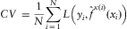
where is an indexing function mapping the partition to which observation i is allocated by the randomisation, and is the fitted function calculated with the k(i) -th subset removed.

For model selection purposes, we do not have a single model to cross-validate but a set of different models indexed by a parameter α, which may represent for example the complexity of the model. For this set of models, we have a different value of CV(α) for every α, and the function CV(α) is effectively an estimate of the test error curve depicted in Figure 1. The optimal model is then , where α* is the value that minimises CV(α).

One key issue with cross-validation is of course the choice of K. Anything from K = 2 to K = N is possible. Typical values are K = 5 and K = 10.

Analytical criteria. The use of the three-set protocol and cross-validation is not widespread among actuaries, and usually limited to practitioners in personal lines insurance. One reason is that many methods that actuaries use for feature selection come with built-in mechanisms to avoid using too many features.

One such mechanism is the Akaike Information Criterion (AIC), which applies to maximum likelihood estimators: adding one parameter to a statistical model can only be justified by a gain in the log-likelihood at least equal to two. Several other analytical approaches are also possible. All of these methods punish complexity, playing the same role as regularisation, and none of them requires validating the model on a different set.

For a better understanding of how these methods work, notice that beside the training error (Equation (1)) and the test error, a.k.a. extra-sample error (Equation (2)), we can define a third type of error, the in-sample error, which gives the distance between the model and an independent sample which shares with the original sample the points at which the model is evaluated. The idea is that part of the discrepancy between the model and the test sample is due to the model being poor, and part is due to the fact that in general the points at which the model is calculated differ from those of the training sample. The in-sample error is defined as

where the is the new response at the same points.

The in-sample error is not a completely satisfactory estimate of model error, and therefore is not completely satisfactory for model validation purposes. However, it usually does a good job for model selection purposes, where the main issue is not the absolute size of the error but how the error of one model compares to the other.

The Akaike information is an estimate of that can be used in the case of a log-likelihood loss function (as is the case for GLM). It can be shown that the following holds:

asymptotically as N→∞. As usual, loglik in the equation above is the maximised log-likelihood. The Akaike Information Criterion for model selection prescribes to choose the model with the smallest AIC over the set of models consideredFootnote 3.

A modified version of the AIC, denoted AICc, has been proposed to deal with the case when the number of data points N is small or the number of parameters d is large:

Using this criterion – which obviously converges to AIC when N→∞ – has been shown to decrease the probability of overfitting. This is also achieved by the Bayesian Information Criterion below.

The Bayesian Information Criterion (BIC) has a similar form to AIC:

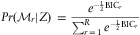
Since the factor 2 is replaced with log N, when the number of data points is 8 or more the penalty for more complex models is larger for BIC for N > 8. It arises in the context of Bayesian model selection, Bishop (Reference Bishop2007), as the posterior probability of a model given a choice among R possible models and training data Z is

Other estimates of the in-sample error can be obtained using the Minimum Description Length (MDL) criterion (Grunwald et al., Reference Grunwald, Myung and Pitt2005), which is formally identical to BIC, and the bootstrap (Hastie et al., Reference Hastie, Tibshirani and Friedman2001).

Comparison of selection/validation methods. We now discuss how the different selection/validation methods compare to one another.

• • AIC and BIC are less general than cross-validation. They can be used in their basic form only for the log-likelihood loss function and when the number of degrees of freedom is defined. For certain nonlinear models, such as neural networks, the number of degrees of freedom can sometimes be replaced with the effective number of parameters (see Hastie et al., Reference Hastie, Tibshirani and Friedman2001). However, for complex models this soon becomes very difficult and AIC, BIC become impractical:

• • the AIC and BIC tend to overestimate the test error by a much larger amount than cross validation. This may be a problem in model selection (but only if this changes the relative order of models) and is certainly a problem in model validation, because the test error is exaggerated;

• • BIC v AIC: BIC is asymptotically correct, in the sense that as the number N of data points tends to infinity, the true model is selected with probability 1. AIC does not have this property, and it tends to favour more complex models when N becomes very large. At the same time, BIC tends to over-punish complexity for finite samples and pick models that are too simple;

• • BIC, AIC are simpler to calculate than cross-validation, as they do not require splitting the data into subsets and calculating the parameters many times.

Cross-validation therefore appears to be a far more general and more rigorous methodology, which however often requires more discipline and extra work.

2.4. Efficiency of model selection/validation methods

A good model selection algorithm should be able to determine what the best model is and what its parameters are in an efficient way – i.e. with low computational complexity.

The brute-force approach to best subset selection, which simply looks all possible combinations of features to choose those to include in the model, is computationally intractable (see Papadimitriou, Reference Papadimitriou1994), as the time it takes to perform the selection increases exponentially with the number of features (“combinatorial explosion’’).

There are two typical approaches to break intractability:

• • Use greedy algorithms: that is, start with a very basic model (for example one that includes no features) and then start adding the features one by one, each time selecting the features that give the most impressive results, e.g. the one that explains most of the variance. This is the approach which is probably the most familiar to actuaries. The problem with this approach is that there is no guarantee that a global minimum (a truly optimal subset of features) will be reached: the order by which we add new features matters (especially when the features are correlated).

• • An alternative to greedy algorithms are the sparsity-based regularisation schemes such as the lasso or elastic net, which will be introduced in Section 4.2. These work by adding a penalty term to the loss function, thus creating a regularised loss function. The size of the penalty term is controlled by a multiplicative parameter. By tuning this parameter, a different subset of features is automatically selected. This is called continuous subset selection and in many cases can be performed quite efficiently, as we will see in Section 2.6.

We now look into the most widespread techniques for feature selection, starting from that which is most popular among actuaries, generalised linear modelling. Regularisation theory and neural networks will also be described, and a comparison between the different methods will then be attempted.

2.5. Model selection by GLM with forward/backward selection

GLM is an extension of the linear model, in which the outputs Y are related to the inputs through a matrix of coefficients β, with the addition of Gaussian noise ε which is usually assumed to be independent of . The extension works by: (i) replacing the simple linear combination of inputs with a linear combination of a wider dictionary of functions , e.g. ; (ii) replacing the Gaussian noise with a more general type of noise, belonging to the so-called exponential family, which includes among the others Gaussian, binomial, Poisson and Gamma noise and is dependent on X; (iii) introducing a further link function g which transforms the responses so as to enforce certain constraints on the output (e.g. positivity). This yields the general form of a GLM:

The parameters of a given model can be calculated by maximum likelihood estimation, or in other words by minimising a log-likelihood loss function:

where the factor “2” has been introduced so as to reduce to the standard squared loss in the case of Gaussian noise.

As an example, claims frequency is usually modelled by a GLM with a Poisson link function and Poisson noise, whereas claims amounts are often modelled using Gamma noise. See Modlin et al. (Reference Modlin, Feldblum, Schirmacher, Schirmacher, Thandi and Anderson2004) for a more thorough discussion.

The specific model for a set of data is usually selected using a greedy approach. This comes in two varieties, forward selection and backward selection. Forward selection starts from the simplest model, Y = constant, and adds at each step the function ψ_j (X _1,…X_n) that reduces the loss function by the largest degreeFootnote 4. Backward selection starts from the most complex model and removes functions one by one: however, this method can only be applied when the dictionary of functions is finite.

To decide whether the selected additional function in forward selection is actually an improvement, a typical test is to check whether the AIC decreases. A simplified, less rigorous test is whether the coefficient of the newly introduced function is significantly different from zero.

2.6. Model selection by regularised regression

The main idea of regularisation as a tool for model selection is that minimising the functional on an independent sample is equivalent to (or rather, can be approximated by) minimising a different regularised functional on the training sample:

(3)

The term is called a penalty term and embeds our prior knowledge on what the desirable features of the parameters are. The most famous example is ridge regression (or Tychonov regularisation), in whichFootnote 5: in this case the idea is that coefficients should be as small as possible.

Although theoretically any loss function could be used in Equation (3), in practice quadratic loss is usually adopted when modelling quantitative (rather than categorical) responses, and most computational methods to derive solutions have been devised for the quadratic loss case.

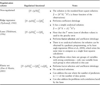
Table 1 shows some examples of regularisation schemes. Ridge regression has a long history, dating back at least to Tychonoff's work on ill-posed problems (Tychonoff, Reference Tychonoff1943), and is probably the best known to actuaries. The reasoning behind this is that in the case of correlated variables, solutions where one large coefficient is compensated by another large coefficient of opposite sign for a correlated variable are common. The l ² penalty term tends to shrink the coefficients, keeping this behaviour at bay, and therefore preventing the inclusion of spurious factors.

Table 1

Examples of regularisation schemes.

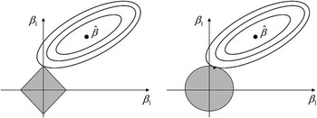
One of the advantages of ridge regression was that an analytical solution is available (see Table 1). As computing power became more easily available, it was possible to experiment with other types of penalty, achieving more sophisticated effects. In 1996 Tibshirani introduced the lasso, a simple modification of Tychonoff's regularisation scheme where the l ₂ penalty term was replaced with an l ₁ term. The loss of the nice analytical properties of the ridge regression is compensated by the fact that the lasso has the (perhaps surprising) effect of enforcing sparsity, i.e. forcing the coefficients of the least important factors to zero and by that keeping the model simple. The underlying reason for this counterintuitive effect is illustrated in Figure 2.

Figure 2

In the figure above, the ellipses represent points for which is constant, whereas the geometric figure around the (0,0) point represents the set of points for which (lasso, left) or (ridge regression, right). The minimisation of the regularised functional is equivalent to the problem of finding β such that is minimal, subject to the condition that . This will occur at a point for which the ellipsis just touches the circle/rhombus. For ridge regression, this intersection point can be anywhere. In the case of the lasso, the intersection is likely to be at one of the vertices for the lasso. This figure is taken from Hastie et al. (Reference Hastie, Tibshirani and Friedman2001, p. 71).

The most significant drawbacks of the lasso are that (Zou & Hastie, Reference Zou and Hastie2005) (i) when the number p of predictors is larger than the number N of observations, the lasso selects at most N variables then saturates; (ii) if there is a group of variables among which the pairwise correlations are very high, the lasso tends to select only one variable from the group; (iii) when large pairwise correlations are involved, the lasso has been shown to perform worse than ridge regression.

These are burning issues in some contexts, such as DNA microarray data analysis, which attempts to find the combinations of genes responsible for a disease. In this case, the number of predictors (genes) is typically larger than the number of observations (DNA samples). Furthermore, some of the genes are highly correlated as they are part of small interacting networks which have to be identified fully to understand the underlying biological mechanism. This has provided the motivation to Zou & Hastie (Reference Zou and Hastie2005) to come up with a regularisation scheme which would overcome lasso's shortcomings while preserving its sparsity-enforcing properties. The results of this effort were the elastic net, which is effectively a hybrid of ridge regression and the lasso and uses a composite l ₂/l ₁ penalty term (see Table 1). De Mol et al. (Reference De Mol, De Vito and Rosasco2009) provided mathematical foundation for this regularisation scheme, showing that the elastic net solution can be interpreted as the fixed point of a contraction in a Banach space, and that under suitable conditions the elastic net estimator is consistent for both prediction and variable selection purposes.

Bayesian interpretation. It should be noted that all the regularisation schemes mentioned above are liable to a simple Bayesian interpretation. In this framework, we are looking for the values of the parameters that maximise the posterior probability given the data, and the penalty term corresponds to the prior probability on the coefficients. The ridge regression penalty term corresponds to a multivariate normal prior probability centred around zero: ; the lasso regression, to a Laplace distribution: ; the elastic net to the distribution . This sheds further light on the nature of regularisation, which is ultimately the incorporation of prior knowledge of the model into the fitting process. The ridge regression reflects the belief that the parameters are small; the lasso reflects the belief that the model is sparse; the elastic net reflects both beliefs.

Applications to general insurance. The lasso provides a simple alternative to the “GLM with forward/backward feature selection” paradigm commonly used in insurance. This way is both rigorous and efficient. As to the drawbacks listed above, the “large p, small N scenario’’ is usually not a concern, at least for personal line insurance applications, but it may become so in applications with sparse data (see Section 2.7 below).

The deterioration of prediction performance in the N > p scenario when highly correlated variables are present is instead something that is quite applicable in our context, as many variables that are considered during the underwriting process, such as the age of the driver and whether the policy purchased is comprehensive or third-party, fire and theft (TPFT) liability only are strongly correlated. An elastic net regularisation scheme might therefore be more adequate in many contexts. The presence of small cliques of predictors that need to be preserved, however, seems to be more specific to biology: there seems no harm in selecting any of a group of correlated variables as long as the overall performance is good.

2.7. Model selection by neural networks

Neural networks were initially developed as simple models for the human brain. The basic units of the network correspond to the neurons, and the connections between these units correspond to the synapses. This provided the inspiration for much research into artificial intelligence, in the hope to emulate the desirable characteristics of the brain, such as Hertz et al. (Reference Hertz, Krogh and Palmer1991): its robustness and fault tolerance; its flexibility and ability to learn; its ability to deal with fuzzy, noisy or inconsistent information.

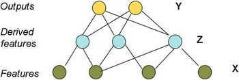
Research on artificial neural networks has gone in waves. The first wave can be traced back to a work by McCulloch & Pitts (Reference McCulloch and Pitts1943), and has culminated in a number of works by Rosenblatt (Reference Rosenblatt1958) in the 1960s on perceptrons, which were networks of neurons organised in layers, such as that in Figure 3, with weights associated with each connection. The first generation of perceptrons – which were single-layered – were found not to be able to perform some elementary computations (Minsky & Papert (Reference Minsky and Papert1969), and research stagnated, until in the mid-1980s the back-propagation algorithm (an example of the gradient descent method) for updating the weights of a multi-layered neural network was discovered by Rumelhart et al. (Reference Rumelhart, Hinton and McClelland1987). Neural networks have ever since been applied to a wide range of problems, from computer vision to particle physics, and as John Denker, an aviation scientist, once famously remarked, they seem to provide “the second best way of doing just about anything’’. Many researchers, however, have found it difficult to accept this paradigm, as the solutions it provides are not transparent - neural networks work, but it is difficult to understand why!

Figure 3

A single hidden layer, feed-forward neural network.

As Hastie et al. (Reference Hastie, Tibshirani and Friedman2001) observe – rejecting both the hype and an outright rejection, neural networks are simply examples of non-linear statistical models, much like project pursuit regression.

Neural networks come in many flavours, the most classical of which is the single hidden layer, feed-forward neural network shown in Figure 3. The single hidden layer, feed-forward neural network shown there can be used for both regression and classification, although for regression there is only one output ( whereas for classification more outputs are needed, the number K of units at the top typically being equal to the number of classes.

The units at the bottom layer are called either features or simply inputs; those in the hidden layer are called hidden units or derived features; and those of the top layer are called either outputs or responses.

Let us outline the main ingredients of the neural network model of Figure 3 and the equations regulating its behaviour:

• • Inputs:

• • Derived features: , where , m = 1,…M. In this equation σ is the activation function. The most popular choice for the activation function is the sigmoid function,

• • Outputs: , where , k = 1,…K. Typically, g(T) = T (identity function) for regression problems.

Solving a problem with a neural network means finding the correct weights to use for a specific problem. The parameters are learned from the data during the training stage, by minimising a suitable loss functions. For regression, this is normally the sum of squares:

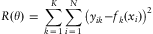
The minimisation can be performed for example by back-propagation, which is an application of dynamic programming.

A key issue with neural networks is that since there are usually many weights there is a danger of overfitting, by adapting too closely to the nuances of the data. To avoid this one can introduce a penalty term and find a regularised solution, for example by minimising . This form of regularisation is called weights decay and is analogous to ridge regression. Alternatively, one can use (as it used to be in the early days of neural networks) an early stopping rule, by which the training of the model is stopped way before a global minimum is reached.

It should be noted that neural networks are very general and that when they include hidden layers they can express any functionFootnote 6 (see the list of examples in Lowe & Pryor, Reference Lowe and Pryor1996). Furthermore, they can be validated like any other method and should not therefore be rejected on the grounds that their results are not reliable.

There is, however, another important reason why neural networks are not suitable for many applications, and it is their lack of transparency: it is difficult to interpret the results of these models. Neural networks “are effective where prediction without interpretation is the goal” (Hastie et al., Reference Hastie, Tibshirani and Friedman2001) – less so when it is important to understand the roles of individual inputs. E.g., they will determine how much a specific customer should be charged, but it will not be obvious what characteristics of the customer have led to that decision. However, the extraction of explanations from neural networks is the topic of active research (see, e.g., Jacobsson (Reference Jacobsson2006), and the very brief discussion of how some authors address the interpretation problem in Hastie et al., Reference Hastie, Tibshirani and Friedman2001).

Applications to insurance. In certain circumstances, the opacity of neural networks may be an advantage as a detailed model specification is not required.

However, the fact that it is difficult to interpret the results of neural networks is certainly a problem in general because they are not going to help us with understanding risk. It is therefore difficult to see how underwriters, managers at an insurance company or the regulator could accept lightly pricing, reserving, capital modelling decisions based on neural networks. Furthermore, they are computationally very demanding.

Despite this problem, some applications of neural networks to general insurance have been attempted, for example by Dugas et al. (Reference Dugas, Bengio, Chapados, Vincent, Denoncourt and Fournier2003), which investigated their use for motor rating in North America. Furthermore, neural networks are routinely used for exploratory analysis as part of data mining and in other financial contexts such as for credit card fraud detection.

Let us now present a simple specific example from general insurance to make it easier to follow the subsequent sections, and go through some general considerations regarding how models should be selected and validated.

2.8. Other methods for supervised learning

This section is a quick foray into a number of more advanced statistical learning techniques, which could be loosely grouped under the header of “kernel methods”. The reader who is keen to explore the topic in more depth is referred to the books by Bishop (Reference Bishop2007), Hastie et al. (Reference Hastie, Tibshirani and Friedman2001) and MacKay (Reference MacKay2003). This section follows mainly Bishop (Reference Bishop2007) (chapters 6 and 7) in the way the material is presented. As usual, we have focused on the problem of regression, although all of these methods can be equally well (and sometimes more naturally, as is the case of support vector machines) used for classification purposes.

Kernel methods

Kernel methods are based on the observation that for many learning algorithms the predicted output is a function of the features (basis functions) built upon the input vector x only through the scalar product . The idea then arises to replace such scalar product with another function k(x,x′) of the inputs which exhibits some desired properties, e.g. to depend only on the distance ||x–x′|| between x and x′. Commonly used kernels are:

• • (linear kernel)

• • (linear kernel – linear in the features space)

• • (stationary kernel)

• • (homogeneous kernel, or radial basis function)

• • (Gaussian kernel – an example of a homogenous kernel)

There are many ways to construct valid kernels (see Bishop (Reference Bishop2007) for a review) and one crucial aspect of this is that kernels can be defined over such disparate objects as sets and graphs.

To see with a simple example how kernels arise in practice, consider a least-squares problem solved with ridge regression, which involves minimising the regularised error function

Given a new input x, the predicted output for such model is

where K is the Gram matrix , an N × N matrix with elements

(4)

and k(x) is the vector whose elements are k(x_n, x). Therefore, the least-squares solution is expressed solely in terms of the kernel function k and the vectors and matrices built upon it. As a result, it is possible to replace the linear kernel with another valid kernel (i.e. a kernel for which the Gram matrix is positive semidefinite) and the solution will still be in the format above. Note that this also makes it unnecessary to introduce basis vectors explicitly.

Gaussian processes

Gaussian processes can be viewed as an application of kernel models: for a Gaussian process, the kernel is simply the covariance function of the predictor. However, Gaussian processes have a more general interest in that they represent a different approach to supervised learning based on a Bayesian framework, and therefore deserve to be given some space on their own.

The ideas around Gaussian processes have been around for a long time and in such diverse fields as geophysics (where Gaussian process regression is called kriging) and control theory (the Kalman filter can be seen as an example of Gaussian process). The most comprehensive text on Gaussian processes is the book by Rasmussen & Williams (Reference Rasmussen and Williams2006). More succinct treatments can be found in MacKay (Reference MacKay2003) and in Bishop (Reference Bishop2007), this paper combines the material in these books.

We saw in Section 2.6 that many regularisation schemes are liable to a simple Bayesian interpretation: a particular choice of the penalty function can be viewed as the imposition of a prior distribution on the parameters of the model in the form (a linear combination of basis functions). The prior distribution incorporates our prior expectations on the model, e.g. that the coefficients β be as small as possible, or that the model is as sparse as possible (fewer basis functions involved).

More generally, in a Bayesian framework the problem of supervised regression can be reformulated as the problem of inferring the true function y(x) based on a set of noisy observations corresponding to input data points where ε_k is random noise. A prior distribution Pr(y(x)) is defined directly over the space offunctions. Upon presentation of a new input x, we can calculate the predictive distribution for y(x) conditional on the data:

(5)

Naturally if our model is parametric, e.g. , the prior distribution on y(x) will simply correspond to a prior distribution Pr(β) on the coefficients β. However, the inference process described above is more general and also holds when Pr(y(x)) is defined on the space of functions directly.

Gaussian processes can now simply be defined as a way of associating a probability distribution Pr(y(x)) over functions y(x) so that the vector of y(x) evaluated at an arbitrary set of points follows a joint Gaussian distribution which is (by definition) completely specified by its mean and covariance matrix. Since we are working in the space of functions, both the mean and the covariance are themselves functions: specifically, the covariance C(x,x′) is a function which expresses the covariance between the values of the function y at points x and x’.

Let us now go back to our supervised regression problem . In a Gaussian process, the error ε_k is itself Gaussian: , where β represents the “precision” of the noise. The joint distribution on the data points conditioned on is again Gaussian and is given by where

(6)

The reason why there are two terms in this covariance matrix is that there are two sources of randomness which are independent: first of all y(x) is a random element in the space of functions (distributed according to a Gaussian distribution by definition) and that of the random noise. Since the two sources of randomness are independent, their covariances simply add up.

The interesting term in equation (6) is the kernel , which is the Gram matrix for the noiseless version of the Gaussian process (ε = 0). For a parametric model using basis functions, e.g. y(x,β) = β ^Tψ(x), the kernel is given by equation (4). However, we can use the kernel trick and replace it with, e.g., a Gaussian kernel or an exponential kernel , obtaining Gaussian processes that do not use basis functions.

We are now in a position to calculate the predictive distribution of t_{N +1} for a new point x given the observations , which is what we set out to do in the first place and for which we have already written down the generic solution in the Bayesian context, equation (5).

It is easy to prove that the conditional distribution is a Gaussian distribution with mean and covariance given by

where

and: C is the matrix whose elements are given by equation (6), k a vector with elements for .

Note that the formulae for the mean and covariance above define the predictive distribution for Gaussian process regression with an arbitrary kernel, the only constraint being that the covariance matrix be positive definite (not semidefinite). For this to be true it is sufficient that be positive semidefinite since the eigenvalues of C are with .

The advantage of such an elegant model as Gaussian process regression is that the output of the regression is not just a number but a full predictive distribution, and the definition of a prior forces analysts to make explicit all the expectations that they have on the types of function that can be fitted to the data (or, expressing this more neutrally, to make explicit all the desired properties of the regression function).

One disadvantage (apart from the obvious limitation that Gaussian processes must be, by definition, Gaussian) is that solving Gaussian processes regression normally involves inverting an N × N matrix (which takes O(N ³) steps) and this is to be compared with the usual basis function model with M basis functions, which takes O(M ³) steps. Typically M << N (the number of model parameters is far smaller than the number of training points) and therefore it is more efficient to deal with basis functions. However, it should be mentioned that (i) what seems like a disadvantage becomes an advantage in the case where the number of basis functions is very large, or actually infinite, and (ii) approximate solutions to the regression problem which are more efficient are available (see Bishop (Reference Bishop2007) for a list of references).

Sparse kernel machines

One of the problems of non-linear kernel algorithms is that needs to be evaluated for each pair of training points, and this may be computationally demanding for large numbers of data points.

A possible way of increasing efficiency is using algorithms for which the solution of the learning problem does not depend on the whole training set but only on a subset of the training points. An example is given by support vector machines (SVM), which owe their name to the fact that the solution depends only on a small number of training points, which are called “support vectors”. A good introduction to support vector machines (and relevance vector machines, which are their Bayesian counterpart) is provided in Bishop (Reference Bishop2007).

SVM for regression is best approached by an example. Let us start by reminding ourselves how linear regression works. In linear regression, the solution to a learning problem is obtained by maximising an error function of the form

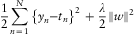
In this formulation, the value of the parameters that minimise the error function will depend on all data points.

Now, let us replace the quadratic term with a function such as

This has the property of being zero when the difference between the model and the target values is smaller than ∈. It is easy to convince oneself that when minimising the error function

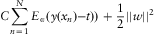
the training points that are within a distance of ∈ from a given model y(x) do not contribute to the error and therefore to the predictions (however, there is a subtlety: it is not possible to say a priori which points can be discarded until the model is actually calculated!). Note how in the error function above the parameter C works as a regularisation parameter, which needs to be determined through cross-validation.

Formally, one finds (see Bishop, Reference Bishop2007) that the prediction for a new input x is

(7)

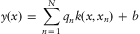
where q_n is zero for all points x_n for which , and k(x,x_n) is given by (4). All the other points x_n are the support vectors of the prediction, and are the only ones for which k(x,x_n) needs to be calculated. As usual, one can perform the kernel trick by replacing the standard form (4) with another positive definite kernel with the desired properties.

The idea of support vector machines has been developed further by the Bayesian community, in order to find a learning algorithm based on the same principle which could produce (as in the case of Gaussian processes) a full predictive distribution as an output, rather than a single number. This has given rise to relevance vector machines (RVM). The general form of the prediction for a new input is Equation (7) as for SVMs: however, the method has certain advantages: (i) there is no regularisation parameter to be optimised; (ii) there is no requirement for k to be positive-definite; and most importantly, (iii) the kernel is usually far sparser than for SVMs (often using a number of relevant vectors which is an order of magnitude lower than the number of support vectors for a SVM).

2.9. Practical general insurance example: rating factor selection for reinsurance

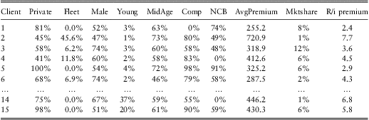
Consider the problem of predicting the reinsurance premium charged for a given layer to different insurance companies for a specific line of business (motor, in this case) based on the profile of the insurer. This is an exercise in second-guessing how reinsurers rate excess-of-loss reinsurance for layers where loss experience is limited.

The factors that define the profile of the insurance company are chosen from a list including:

• • percentage of private (v commercial) vehicles

• • percentage of comprehensive (v TPFT) policies

• • percentage of male drivers

• • percentage of young drivers (≤25 y.o.)

• • percentage of mid-age (26-… ) drivers

• • percentage of drivers with ≥60% no-claims discount

• • Average direct (original) premium

• • Market share

• • …

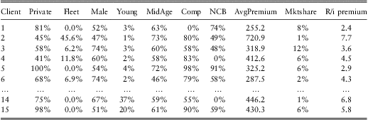
The input is in the form of a table such as that shown in Table 2. This table is based on real data but have been scrambled and scaled beyond recognition.

Table 2

Reinsurance premium xs £5 m and possible rating factors for different insurance companies. Figures are based on real data but are scrambled and randomised beyond recognition.

This is not a very sophisticated example and a multivariate Gaussian model of the linear variety will suffice: i.e., we model the reinsurance premium Y as a linear function of the rating factors:

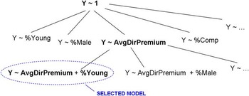
GLM approach. The standard approach to this problem with GLM is through forward or backward selection of the best model. Forward selection is a form of greedy approach and starts with the simplest model (in our case, in GLM shorthand), then adding at each step the variable which reduces the variance between the model and the empirical data by the largest amount, until the addition of a new variable does not add a statistically significant advantage. Backward selection (which will not be used here) works the other way round, starting from the complete model (that where all the variables are included) and removing one variable at a time.

Figure 4 shows the application of the forward selection model to our case, which leads to the selection of the model . Table 3 provides the background numbers for this choice.

Figure 4

Illustration of the forward selection method.

Table 3

Increasingly complex models for the reinsurance premium, and their statistical significance. Every time the variable that explains most of the residual variance is added to the model, the variance is reduced. The column Pr(>∣t∣) gives the probability that the ratio between the coefficient and the standard error of the latest variable added is larger than ∣t∣ by chance although the true value of the coefficient is zero. A value above a significance value of 5–10% indicates that the coefficient is not significantly different from zero. More rigorously, the drop in variance obtained by the addition of a new variable is statistically significant only if the value of AIC (fourth column) decreases. Both these criteria indicate in this case that the best model is .

The main problem with this approach lies in the model selection process, which does not guarantee that it will not fall into local minima, and is relatively inefficient.

Regularisation approach. We now use a simple lasso regularisation approach to solve the same problem. We use an R package called “LARS”, authored by Hastie & Efron (Reference Hastie and Efron2012). This package performs an automatic selection process which is guaranteed to find the global minimum, and it does it within the time it takes to do a single least square regression.

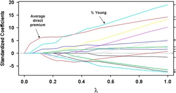
The coefficient values are plotted against the regularisation parameter λ, which is expressed as a fraction of , where is the least squares estimate of coefficient Note that when the regularisation parameter becomes larger than t*, the lasso estimates coincide with those of least squares regression. Owing to the nature of the lasso, the coefficients are all zeros when λ = 0, then as we increase λ the coefficients become positive one by one, as in Figure 5.

Figure 5

Illustration of the least-angle regression method (LARS) to generate all lasso solutions for different values of the regularisation coefficient.

As Figure 5 shows, the first coefficient to become non-zero is that for the average direct premium, and the second is that for the percentage of young drivers, then all the others, one by one.

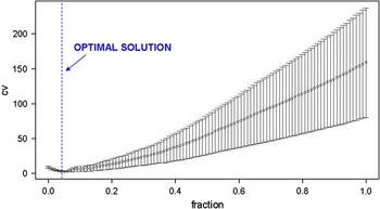
The same package offers a method to decide which value of λ should be selected based on cross-validation, as shown in Figure 6, which gives the expected prediction error as a function of the value of λ, again expressed as a fraction to the largest coefficient.

Figure 6

Expected prediction error for different values of the regularisation parameter, obtained through cross validation.

The minimum value of the prediction error is obtained around 0.05. This corresponds to including the variables ADP and %Young, exactly as for the GLM model. The model has however been obtained effortlessly and is guaranteed to yield the global minimum.

2.10. Comparison of different techniques for supervised learning

We now summarise our considerations on the different techniques for supervised learning that we have investigated so far, in order to give an at-a-glance comparison among these techniques.

Neural networks

• • Neural networks are very flexible: they are not limited by linearity and they can express any function of the data.

• • Neural networks do not require any model specification, and are therefore easy to implement.

• • A key disadvantage of neural networks is that they provide “prediction without interpretation”: the output of a risk costing exercise are the values assigned to the weights of the network, which have no intuitive meaning. This does not mean that they are any less rigorous than GLM or regularisation: their models can be validated exactly in the same way. However, they do not help us understand risk and this makes their acceptance by underwriters, management and regulators problematic.

• • Neural networks are computationally demanding: training them takes a fair amount of time.

Generalised linear modelling

• • The loss function can be chosen to reflect (to some degree) the underlying process noise.

• • Generalised linear models are easy to interpret: the factors included in the model are those that have a significant impact on the risk, and the chosen functional dependency (e.g. exponential, polynomial) is usually simple.

• • Generalised linear models are limited by linearity. However, in practice, a large dictionary of functions is possible and linearity in the coefficient will seldom be impairing.

• • Model selection with forward or backward selection is computationally awkward and may get trapped in local minima.

• • Standard methods for model validation (as those based on AIC) may overestimate the test error.

Regularised regression

• • Feature selection is completely automated, and a global minimum is guaranteed to be reached. Model selection and validation can be performed very efficiently, avoiding the combinatorial explosion of best subset selection.

• • The interpretation of regularisation results is easy as for GLM.

• • Specific types of regularisation such as the elastic net can address the problems arising when there are highly correlated variables and when the number of predictors exceeds the number of available data points.

• • The use of quadratic loss function for classical regularised regression is limited and causes degradation of performance with some types of noise. This has been demonstrated in Parodi (Reference Parodi2009)with the use of artificial data for the case of Poisson noise: the expected prediction error increases as the Poisson rate of the underlying processes decreases (this makes sense as for large Poisson rates the distribution of the number of losses will be near-Gaussian).

• • A different loss function can be used, but some of the theoretical results obtained for squared loss may be lost, and the solution may not be as simple (see Rosasco et al., Reference Rosasco, De Vito, Caponnetto, Piana and Verri2004).

The comments above reflect the “textbook approach’’ of the relevant methodologies. It is fair to mention, however, that these methodologies come in many flavours and that hybrid approaches are possible and have actually been attempted. As an important example, GLM can be coupled with regularisation: see for example Park & Hastie (Reference Park and Hastie2007), where l ₁–regularization (lasso) was applied to a log P loss function. In the author's opinion this is one of the most promising avenues that actuaries should explore.

Also, cross-validation is used more in the context of neural networks and regularised regression than in the context of GLMs, but there is no reason why it should not be used for GLM as well. In a paper presented last year by a general insurance research organising (GIRO) working party (see Berry et al., Reference Berry, Hemming, Matov and Morris2009), the use of a hold-out sample was advocated as an important validation tool.

2.11. Dealing with sparse data

It is fair to mention at this point that most techniques discussed in this section work best when there is a large amount of data to play with. Indeed, techniques such as GLM are mostly used in personal lines insurance where the quantity of data is not an issue. However, statistical learning can in principle be applied as well where data are sparse, and some techniques have either been developed exactly to deal with the data sparsity issue or they help address data scarcity.

More specifically:

• • some regularisation techniques such as the elastic net were devised to address the problem where the number of data points is much smaller than the number of explanatory factors (a clear case of data sparsity, and a counterintuitive one);

• • in at least one context where data sparsity is almost physiological, i.e. the modelling of large losses, extreme value theory provides theoretical constraints on the type of models that can be fitted (e.g. a generalised Pareto distribution must be used to model the severity of losses above a large threshold). This has an interesting interpretation in terms of statistical learning, as one of the methods to avoid overfitting is to limit the number of models that one can choose from. In the case of EVT, the model selection phase can actually be skipped altogether and we can jump straight to model parameterisation and model validation;

• • if we adopt a Bayesian approach to statistical learning, it is possible to incorporate the prior probability of models (see II. Dealing with uncertain knowledge, Section 2.4), and also to incorporate expert judgment. In this context, statistical learning provides a way of making up for the lack of data by tilting the balance away from the actual experience and towards prior or external knowledge.

The issue of the sparsity of data and how statistical learning can help with it was recently addressed in a talk at GIRO (see Chhabra & Parodi, Reference Chhabra and Parodi2010).

3.1. Clustering techniques

One possible categorisation of clustering techniques is this:

• • Partitioning techniques (K−means, K-medoids, EM), which partition data based on a given dissimilarity measure.

• • Hierarchical methods, which subdivide data by a successive number of splits.

• • Spectral clustering, which works by graph partitioning techniques after a transformation into a suitable space.

• • Dimensionality reduction techniques (principal component analysis, self-organising maps (SOMs), generative topographic mapping, principal component analysis, etc), which are based on the observation that often the data points lie in (possibly non-linear) low-dimensional manifolds embedded in a data space with many more dimensions.

• • Other: density-based methods, grid methods, kernel clustering. These will not be dealt with here.

We are going to look at each of them in turn.

Partitioning techniques. Partitioning techniques subdivide data based on a given (dis)similarity measure. The most popular algorithm for clustering is perhaps K-means, as it is simple and intuitive.

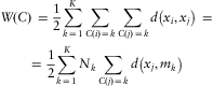
The dissimilarity measure for K-means is typically (but not necessarily) the squared Euclidean distance (notice that x_i and x_j are in general vectors in ).

The aim is to minimise the within-cluster point scatter:

The method works iteratively by

1. 1. Choosing the number K of clusters

2. 2. Choosing randomly (or cleverly) K data point as the initial cluster means m_k

3. 3. Assigning each object x to the closest cluster mean

4. 4. Updating cluster means by minimising W(C) with respect to the m_k's

5. 5. Iterating steps 3 and 4 until assignment does not change

This method's advantages are that it is easy to understand and apply. Also, it always converges quickly. However, it has several disadvantages:

• • the number of clusters must be decided in advance. Different values of K have therefore to be tried to check which value gives the “best” results;

• • in case the Euclidean distance is used, the method is sensitive to noise, as the sum of the squared distance between points may be overly influenced by a few data points with larger distance;

• • the algorithm may get stuck in a suboptimal local minimum. As regards to this, the choice of the initial clusters is crucial;

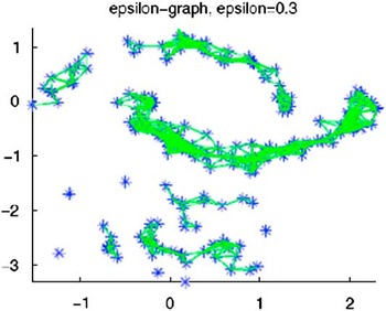
• • clusters lie in disjoint convex sets of the underlying space. This may be a disadvantage when the actual shape of the “real”‘ clusters is unusual, as in Figure 7;

  Figure 7

  The clusters in this figure are not convex. This will cause problems with k-means. The clusters here are obtained using spectral clustering (explained later on in this section).

  

• • there are issues when the density of different clusters is not uniform.

Examples of other partitioning methods (besides K-means) are K-medoids and expectation maximisation. K-medoids is very similar to K-means, but rather than choosing freely among points in the underlying space to be the cluster means, it always chooses one of the actual points in the dataset. Expectation maximisation is a ubiquitous technique in statistics, that can be applied to a number of contexts, including clustering. See for example Hastie et al. (Reference Hastie, Tibshirani and Friedman2001) for an explanation.

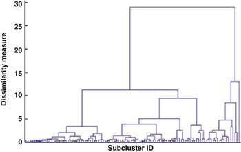
Hierarchical methods. Hierarchical methods use cluster-to-cluster similarity in order to decide whether to merge/split clusters. They create a hierarchical decomposition forming a dendrogram (a tree that splits recursively). The idea behind a dendrogram is that depending on the dissimilarity threshold at which you decide that two clusters should be merged (y–axis), the number of clusters (i.e., the number of vertical lines crossed by a line with constant y varies. An example of a dendrogram is shown in Figure 8.

Figure 8

An example of dendrogram [modified from Yao paper, Yao, Reference Yao2008]. Notice how the number of clusters depends on the dissimilarity measure at which two dendrograms are split.

Hierarchical methods have some similarity with rule-induction systems, which segment data according to their attributes, e.g. based on a number of “If-Then” conditions applied to each attribute in turn (see, e.g., Liang, Reference Liang1992).

One advantage of hierarchical methods is that – unlike K-means – they do not commit to a number of clusters K in advance, giving them more flexibility. Also, they are easy to understand (the dendrogram provides a highly intuitive description of the product of hierarchical clustering at different levels of dissimilarity) and apply.

One disadvantage is that the dendrogram does not provide any clear decision criteria – judgment must be used to select the threshold of the dissimilarity measure which will then produce a specific clustering.

Spectral clustering. Spectral clustering is becoming one of the most popular techniques in clustering, owing to its flexibility, its efficiency and its theoretical elegance. Only a cursory overview will be given here, but the interested reader will find an entertaining reference in the tutorial by von Luxburg (Reference von Luxburg2007).

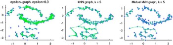
Spectral clustering has its roots in graph theory, and its central idea is to solve the problem of clustering not in the original space (as K-means does) but on a transformed space embedded in a graph, the so-called similarity graph. The similarity graph is a graph whose vertices are the data points and two data points are connected by an edge if they are similar, as in Figure 9. The similarity function is somehow related to the “distance” between the points in a suitable space. For example, in a Euclidean space the similarity function might be defined as . Finding the clusters in the data set is then equivalent to finding partitions (groups of vertices) in this graph which are weakly connected to each other but whose vertices are very similar inside.

Figure 9

Different types of similarity graph: ε-neighbourhood graph (left), k-NN graph (centre), mutual k-NN graph (right). The difference between k-NN and mutual k-NN is that in the latter we include an edge between vertices v_i and v_j only if the vertices are both among each other's k nearest neighbours. Notice the non-convex shape of the clusters and the fact that the clusters have different densities. The figure is borrowed from von Luxburg (Reference von Luxburg2007).

The essential aspect of spectral clustering is how you build the similarity graph, so it is perhaps worth spending a few words on this. Three types of similarity graphs are commonly used:

• • the ε-neighbourhood graph, in which every pair of vertices for which the similarity function is larger than ε is connected (see Figure 9(left)). This graph is usually unweighted;

• • the k-nearest neighbour graph, in which the k nearest neighbours of a given vertex are connected to that vertex (see Figure 9(centre and right). This type of similarity graph is useful especially when we have clusters at different scales - that is, one cluster may be denser, the other more rarified, as in Figure 7;

• • the fully connected graph, in which all vertices are connected. This graph will obviously be weighted and the weighting should decay exponentially, thus effectively defining a neighbourhood radius.

One version of the spectral clustering algorithm (“unnormalised spectral clustering”) works as follows:

1. 1. Build the similarity graph G = (V, E) where are the vertices (the data points), E is a set of edges, i.e. a subset of V×V (pairs of vertices). The graph is assumed to be undirected. If the graph is weighted, that means that every edge (v _i, v_j) will have an associated weight w_i,j. The matrix is called the weighted adjacency matrix.

2. 2. Calculate the graph Laplacian , where W is the adjacency matrix defined above and , where . The laplacian has many interesting properties: for example, it is symmetric and positive semi-definite, and has n non-negative, real-valued eigenvalues . The multiplicity k of the eigenvalue 0 of equals the number of connected components in the graph.

3. 3. Calculate the first k eigenvectors of and build the matrix (columns) (rows).

4. 4. Group points -means

This algorithm produces sensible clusters, but it is not obvious why! Several arguments have been put forward to explain why spectral clustering works: see for example von Luxburg (Reference von Luxburg2007). The perturbation theory argument is probably the most intuitive, and can be outlined as follows.

Perturbation theory studies how the behaviour of eigenvalues and eigenvectors changes if one applies a small perturbating matrix H to the original matrix A. This may help us understand the workings of spectral clustering by considering the ideal case – that is, the case where the clusters are already perfectly separated at the stage when one builds the similarity graph. In this case, the points built by the algorithm above will have the simple form (0,…0,1,0,…0), and the position of the 1 indicates the connected component this point belongs to. All the vectors belonging to the same connected component are coincidental, and identifying the clusters is trivial.

If we now perturb the original matrix by a small amount, the points y_i will not be exactly -means algorithm will still find the same clusters.

The pros and cons of spectral clustering as listed below are mostly borrowed from von Luxburg (Reference von Luxburg2007).

• • No strong assumptions on the shape of the clusters are needed. In particular, it is not necessary for clusters to be convex in the original space (see for example the moon-slice-shaped clusters in Figure 7).

• • Spectral clustering is efficient on sparse graphs -- of course, it is up to us to ensure that we choose the similarity graph so that it is sparse!

• • Finding the solution given the similarity graph is a linear problem and therefore one cannot get stuck in local minima. Also, it is not necessary to restart the algorithm several times with different initial values, as for many other clustering methods.

• • On the downside, the choice of a good similarity graph is crucial and not always easy. It is unstable under different choices of the parameters for the neighbourhood graph. All this amounts to saying that spectral clustering cannot be used as a black box!

• • Spectral clustering may be difficult to understand/communicate: the very reason why it works is not obvious. However, its obscurity is not of the same type as that of neural networks, because here it is clear what the algorithm is trying to achieve – finding clusters on the similarity graph rather than on the original space.

Dimensionality reduction techniques. These techniques are based on the observation that data points, although they may live in a data space with many dimensions, in practice may all lie close to a low-dimensional manifoldFootnote 7 embedded in the data space.

As an example, buyers of house insurance may be described as points in a space with as many dimensions as there are rating factors that have been collected – say 20 or more of them: however, in practice you may find that certain rating factors which you have zealously collected (e.g., the current colour of the house) end up being not material, or that only certain combinations of the values of the factors occur in practice.

Sometimes the underlying manifold is a linear manifold, i.e. it is a linear subspace of the data space. In this case linear modelling techniques suffice to discover this subspace. An example of these techniques is given by principal component analysis (PCA), which projects all the data points onto a principal subspace with some optimisation criterion, e.g. the subspace that captures most of the variance. PCA comes in many fashions: straight PCA, probabilistic PCA, EM PCA, Bayesian PCA, factor analysis, kernel PCA (see Bishop (Reference Bishop2007) for a short review).

In general, the manifold around which the data lie will not be linear, and nonlinear techniques are therefore needed. This can be dealt with by, e.g.,

• • approximating the non-linear manifold with a piecewise linear manifold (e.g. approximating a hypersurface locally with hyperplanes);

• • using self-organising maps (aka Kohonen maps). A self-organising map represents a 2D nonlinear manifold as an array of discrete points, called prototype vectors. Initially, these prototype vectors are distributed at random, but during training they “self organise” (hence the name of this technique) into a discrete rendition of a low-dimensional smooth manifold. One disadvantage of this technique is that there is not a clearly defined cost function that can be minimised and according to which convergence can be assessed. The next technique, generative topographical mapping, is a variant of SOMs that addresses this problem;

• • using generative topographical mapping (GTM). This is a probabilistic version of the self-organising maps mentioned above, and produces a probability density in the data space made up of a mixture of Gaussian distributions with the same variance and with means lying on a smooth two-dimensional manifold. The “optimal” mixture corresponds to the maximum of a log-likelihood function.

The reader who is interested in more detail on these techniques is referred to Bishop (Reference Bishop2007) and to the literature cited therein.

3.2. Practical general insurance example: Clustering for IBNER data

A possible application of unsupervised learning is to IBNER analysis. The underlying problem is that of predicting the ultimate value of a claim (or a probability distribution) given its previous history of paid and incurred amounts. An example is shown in Figure 10.

Figure 10

The history of a claim occurred in 2000 and reported in the same year. For each year of development, the paid, outstanding and incurred (estimated) amounts are given. The outstanding ratio (outstanding amount divided by incurred amount) is also given for each year. The last row shows the IBNER factors for this claim, calculated as the ratio between the incurred amounts of two successive years. The claim shown here is a real claim after scaling by a random amount and the removal of any identifiable information.

The numerical example illustrated here was analysed with the help of Nicola Rebagliati, from the Department of Computer Science of the University of Genoa.

For pricing or reserving purposes, especially for large losses, one often looks at the distribution of past IBNER factors to predict the ultimate value of a particular claim or to put aside some IBNER reserves. The idea is that by spotting a systematic bias (on average) on the claims estimates, the estimates can be put right (again, on average!) by correcting all claims with the same characteristics.

The calculation of IBNER factors is usually performed by chain ladder calculations (or something similar) and often a simple average over all open claims (settled claims will of course have no IBNER, unless they are re-opened) is all that is used, especially if the number of individual claims histories is not large: the output of such analysis would then be an IBNER factor which depends only on the development year.

However, it is obvious that the IBNER factor will depend in general on many factors, such as:

• • development year (the younger the claim, the more scope there is for it to deviate from the incurred estimate), as already mentioned;

• • size of claim (larger claims may have more uncertainty about them);

• • outstanding ratio (the larger the outstanding amount, the more conjectural the estimate of the incurred value will be);

• • type of claim (for example, bodily injury claims will be more difficult than property claims to estimate reliably as the victim's health may worsen unexpectedly);

• • reserving style (claims managers may be more or less effective at reserving, and some may introduce a systematic upward/downward bias);

• • …

As in all situations in which one needs to understand how different factors impact a given variable, one can use the data set to perform supervised learning as in Section 2 (“Learning from data”). However, not all the variables in the list above lend themselves to be used easily as input variables: specifically, the “reserving style”‘ above is quite difficult to use as the claims history is a vector of, say, 15 years of development.

One possible solution is to collect all individual claims development histories and group them into clusters of similar behaviour. Once clustering is performed, the cluster ID can be used as one of the rating factors in a regression exercise with GLM or regularisation.

One complication of this exercise is that different claims histories will have different lengths (some may be 2 years long, some 15) and therefore one must put a little care into how one defines a similarity measure. Since here we are only interested in giving an illustration of various applications of clustering, we will limit ourselves to extract sections of claims histories of exactly 5 years (the history of the claim may go on after 5 years, but we look at a section of the data spanning 5 years only).

The data used are large motor losses from several UK insurers. The losses have been normalised so that the latest known incurred value (not necessarily that at the fifth year) is set to 1 -- which makes them unrecognisable and removes the dependency on loss size.

Figure 11 shows a few examples of the claims histories we are trying to cluster, after normalisation.

Figure 11

Examples of loss progressions. The most recent estimate of the claim (possibly beyond the 5-year horizon) is normalised to 1.

The clusters were obtained with a simple K-means algorithm. A value of K = 10 was chosen, which gives good results in terms of separation of clusters. The cluster means are shown in Figure 12.

Figure 12

Cluster centres for the clusters calculated with K-means, k = 10.

Notice that these clusters can be interpreted as follows:

• • cluster 6 is the most typical behaviour and occurs when the estimate of the incurred amount is quite stable after an initial 8% increase. Cluster 7 is also relatively stable but it starts with a 30% over-reserving;

• • cluster 8 shows a typical pattern of under-reserving;

• • clusters 1, 2, 4, 5, 9, 10 are typical patterns of over-reserving;

• • cluster 3 shows claims for which the incurred amount has returned to the initial value after a period of over-reserving.

It is interesting to compare these clusters with a piece of information that we have not used in the clustering process – the name of the company that reserved those claims. The results of this comparison are shown in Figure 13. It is clear that certain companies (such as Company J) have a higher-than-average tendency to under-reserve.

Figure 13

The percentage of each type of cluster for a selection of UK companies.

It is interesting to compare these results with those one obtains with spectral clustering. To use spectral clustering, we first have to choose a similarity graph. One choice is the ε –neighbourhood graph with similarity function , where ||x_i–x_j|| is the distance in between our vectors representing the development of claims. However, this is going to give results very similar to the K-means algorithm tested above.

We have therefore used the k-nearest-neighbour similarity graph.The choice of k is of course crucial. Unfortunately, there are few theoretical results guiding us in the choice of k. A few heuristics are often recommended, though. One is that k be chosen so that the resulting similarity graph is connected, or that the number of connected components is less than the number of expected clusters – otherwise there is a danger that the algorithm will simply return the connected components as clusters. For very large graphs, a rule of thumb is to look at values of k in the region of log n(n being the number of data points). In our case, this does not give sensible results.

Another option is to look at the so-called Laplacian spectrum, which gives (for a given number of k of the kNN graph) the value of all the n eigenvalues (some of them possibly repeated if their eigenspace has dimension >1) in decreasing order. In the ideal situation we would have only K eigenvaluesFootnote 8 that are near zero and can therefore be considered—from a perturbation theory point of view – as “noisy’’ versions of the first eigenvalue λ₁= 0 of multiplicity K. Then there should be, always in the ideal case, a gap between the K-th and the K+1th eigenvalue,related to the gap between λ ₁ and λ ₂.

After trying out several values of k, we have found that we need to go up to about k = 300 to have the appropriate structure of the graph, and the Laplacian spectrum indicates that a reasonable choice for the number of clusters is 5. See Figure 14 for examples of Laplacian spectrums.

Figure 14

Left. Laplacian spectrum for the k-nearest-neighbour similarity graph, k = 20. No structure is apparent in the graph and there is a large number of eigenvalues near zero, without a clear difference between the near-zero behaviour and the rest. It is therefore not possible to identify a small number of eigenvalues that are near-zero. Right. Laplacian spectrum for the k-nearest-neighbour similarity graph, k = 300. The structure is better and there are only a few eigenvalues below 0.5 (five of them). There is then a significant gap between the fifth and the sixth eigenvalue. This structure therefore suggests the existence of five clusters (but anything between 3 and 5 would be acceptable).

Notice that the selected number (k = 300) is quite an extreme choice for the number of nearest neighbours in the similarity graph. The underlying reason might just be that there are no natural clusters in this IBNER problem, because the patterns in IBNER development are not sharply defined. However, the existence of a few (3-5) patterns is indeed confirmed by a comparison of the results of spectral clustering and K-means, and by looking at which clusters are more common for each company.

These results are shown in Figure 15, which shows the centres of the five clusters found with spectral clustering, and in Figure 16, which shows the percentage of each cluster for each company. There is indeed a striking similarity with the results obtained with K-means: in both cases, we have an important cluster collecting all the claim developments that are stable (cluster 6 for K-means and cluster 5 for spectral clustering). Also, in both cases we have a single cluster which attracts all claims that are under-reserved and sometimes keep growing year-on-year. The other clusters are in both cases mostly examples of over-reserving and could easily be further aggregated. The main difference is the presence in K-means of a cluster (cluster 3) that starts from 1, goes up to 1.3 and goes back to 1 again -- however, this is likely to be an artifact, and spectral clustering is probably right in ignoring it.

Figure 15

Cluster centres for the clusters calculated with spectral clustering. A k -nearest-neighbour similarity graph has been used, with k = 300.

Figure 16

A comparison of a few companies (after scrambling, and selection of the first half of them, to make them fully unrecognisable).

Overall, there seems to be some improvement with respect to K-means. However, it should be mentioned that in this example the clusters are probably already convex in the original space, and clusters are not sharply defined because claims developments vary over a continuous range.

Although in this case the difference between K-means and spectral clustering is not striking, spectral clustering is a far more flexible method (which incorporates K-means anyway in the standard implementation of the method) and despite the fact that it takes a while to explain, it is quite simple to implement, it is very efficient and has some important properties (local minima, convexity in the appropriate space). It is therefore something that actuaries should consider alongside K-means when doing clustering, especially when the structure of their data is complex, before concluding that clustering does not help them.