1. INTRODUCTION
Spin stabilisation is a common attitude control method for spacecraft (Soken et al., Reference Soken, Sakai, Asamura, Nakamura and Takashima2016). It is usually used on micro-satellites and nanosatellites for its simple implementation and low-energy cost (Slavinskis et al., Reference Slavinskis, Kvell, Kulu, Sünter, Kuuste, Lätt, Voormansik and Noorma2014). In 1993, Markley proposed variables including seven angular momentum parameters to estimate the attitude of spinning spacecraft (Markley, Reference Markley1993); these vary slowly and are easy to integrate numerically (Sedlak, Reference Sedlak2005). The attitude estimation methods using Markley variables are given the generic name Spin Kalman Filter (SpinKF). Some different versions of SpinKF can be obtained depending on the choice of the error state. When the angular momentum error vector in the inertial reference frame is chosen, the SpinKF is called SpinKF-I, where I refers to the inertial reference frame. Whereas when the angular momentum error vector in the body reference frame is chosen, the SpinKF is called SpinKF-B, where B refers to the body reference frame. (Markley and Sedlak, Reference Markley and Sedlak2008). Markley and Sedlak (Reference Markley and Sedlak2008) illustrated that SpinKF-I shows a better robustness and efficiency than some other methods. The attitude estimation methods based on Markley variables for spinning spacecraft often employ a combination of magnetometer, sun sensor and gyro (Sedlak, Reference Sedlak2005; Markley and Sedlak, Reference Markley and Sedlak2007; Reference Markley and Sedlak2008; Ha, Reference Ha2010). However, a star sensor can replace the combination of a magnetometer, sun sensor and gyro by using a star vector and optical flow as measurement. Optical flow is defined as a Two-Dimensional (2D) rate vector which arises from either the motion of the objects in the scene or the motion of the sensor (Kumar et al., Reference Kumar, Kumar and Raman2016). The motion can be calculated using optical flow between two image frames or a sequence of frames without any prior knowledge (Chen et al., Reference Chen, Kang and Park2013). Optical flow has been used on the angular rate estimation of three-axis spacecraft (Fasano et al., Reference Fasano, Rufino, Accardo and Grassi2013; Pal and Bhat, Reference Pal and Bhat2013). Similarly, optical flow can also provide rate information on the attitude estimation for spinning spacecraft.
This paper presents a Markley variables-based attitude estimation method for spinning spacecraft using optical flow and a star vector from a star sensor. Simulations show that the estimation accuracy of the spin axis and spin angular rate can be improved by using optical flow and a star vector as measurements.
2. SYSTEM MODELS OF THE MARKLEY VARIABLES-BASED ATTITUDE ESTIMATION METHOD USING OPTICAL FLOW AND STAR VECTOR
2.1. State model
The Markley variables include LB, L I and ζ. LB and LI are the angular momentum of the spacecraft in the body frame and inertial frame, respectively. ζ is the rotation angle of the spacecraft. The Markley variables LB, LI and ζ obey the following equations of motion (Sedlak, Reference Sedlak2005; Markley and Sedlak, Reference Markley and Sedlak2008):
 $$\eqalign{\dot{\bi L}_{B} &= N_{B} - {\bf \omega}_{BI} \times {{\bi L}}_{B} \cr \dot{\bi L}_{I} &= {\bi N}_{I} = {\bi R}_{BI}^{T} {\bi N}_{B} \cr \dot{\zeta} &= \displaystyle{L[({{\bi L}}_{B} + {{\bi L}}_{I}) \cdot {\bf \omega}_{BI} + L^{-2} ({{\bi L}}_{B} \times {{\bi L}}_{I}) \cdot ({{\bi N}}_{B} + {{\bi N}}_{I}) \over L^{2} + {{\bi L}}_{B} \cdot {{\bi L}}_{I}}}$$
where NB and NI are the total external torque of the spacecraft in the body frame and in the inertial frame, respectively. ωBI = [ω 1 ω 2 ω 3]T, ω1, ω2 and ω3 are the angular rate of the spacecraft around the x-axis, y-axis and z-axis in the body frame, respectively. ωBI can be given by:
 $${\bf \omega}_{BI} = {\bi J}^{-1} ({\bi L}_{B} - {\bi h})$$
where J is the spacecraft moment of inertia tensor and h is the angular momentum relative to the spacecraft of any moving components (reaction wheels, antennae or solar arrays, etc).
In Equation (1), L = ‖LB‖ = ‖LI‖. RBI is the inertial-to-body attitude matrix of the spacecraft (He et al., Reference He, Yan, Sun and Chen2017), which can be obtained by two rotations based on the Markley variables as follows:
 $${\bi R}_{BI} = {\bi R}_{2} {\bi R}_{1}$$
According to the representation of a rotation matrix based on the Euler axis/angle (Shuster, Reference Shuster1993), we have:
 $${{\bi R}}_{1} = (\cos \zeta) {{\bi I}}_{3 \times 3} + (1 - \cos \zeta){{\bi L}}_{Ie} {{\bi L}}_{Ie}^{T} - (\sin \zeta)[{{\bi L}}_{Ie} \times]$$
 $${{\bi R}}_{2} = ({{\bi L}}_{Be} \cdot {{\bi L}}_{Ie}){{\bi I}}_{3 \times 3} - {{\bi L}}_{Ie} {{\bi L}}_{Be}^{T} + {{\bi L}}_{Be} {{\bi L}}_{Ie}^{T} + (1 + {{\bi L}}_{Be} \cdot {{\bi L}}_{Ie})^{-1} ({{\bi L}}_{Be} \times {{\bi L}}_{Ie}) ({{\bi L}}_{Be} \times {{\bi L}}_{Ie})^{T}$$
where the unit vectors of angular momentum are LBe = LB/L and LIe = L I/L. [LIe × ] is the cross-product matrix.
The state vector is  ${\bi X} = [{\bi L}_{B}^{T}\;\; {{\bi L}}_{I}^{T}\;\; \zeta]^{T}$. According to Equation (1), the state model based on Markley variables with process noise w(t) can be abbreviated as:
 $$\dot{\bi X} = f({\bi X}, t) + {\bi w}(t)$$
2.2. Measurement model of optical flow
The rotation of a spacecraft carrying a star sensor will make the star on the image move from one point to another. The movement of the star points generates optical flow of the star image. Thus, optical flow is considered as a 2D rate vector of stars in a star image which arises from the motion of a star sensor.
2.2.1. Measurement acquisition
Assuming there are m matching stars in two successive star images, the image coordinates of the ith star at time t k and t K−1 are [x i(k), y i(k)] and [x i(k − 1), y i(k − 1)] (i = 1, 2, …, m), which can be obtained through star centroid extraction and star matching. The optical flow (u i(k), v i(k)) of the ith star at time t k can be acquired from two successive star images at time t k and t k−1 by differentiating the star coordinates as follows:
 $$\left[\matrix{u_i (k) \cr v_i (k)} \right] = \left[\matrix{\dot{x}_i (k) \cr \dot{y}_i (k)} \right] \approx \displaystyle{1 \over \Delta T} \left[\matrix{x_{i}(k) - x_{i}(k - 1) + \varepsilon_{x_i} (k) - \varepsilon_{x_i} (k - 1) \cr y_{i}(k) - y_{i}(k - 1) + \varepsilon_{y_i}(k) - \varepsilon_{y_i} (k - 1)} \right]$$
where the sampling period of the star sensor is ΔT = t k − t k−1.  $\varepsilon_{x_{i}}$ and
 $\varepsilon_{y_{i}}$ are the measurement noise in the x and y directions, respectively. Therefore, the measurement vector Z1(k) using the optical flow of stars is:
 $${{\bi Z}}_{1}(k) = [u_{1}(k)\;\; v_{1}(k)\;\; u_{2}(k)\;\; v_{2}(k)\;\; \cdots\;\; u_{m}(k)\;\; v_{m}(k)]^{T}.$$
2.2.2. Measurement model
The coordinates of a unit star vector (rc) in a camera frame are [X c, Y c, Z c]T and its 2D image coordinates in a star image are [x, y]T. In the pinhole camera model, the relationship between x, y and rc is:
 $$\eqalign{x &= -f \displaystyle{X_{e} \over Z_{e}} \cr y &= -f \displaystyle{Y_{e} \over Z_{e}}}$$
where f is the focal length of the star sensor.
The movement equation of the spacecraft (Pal and Bhat, Reference Pal and Bhat2013) is:
 $$\dot{\bi r}_{c} + {\bf \omega}_{BI} \times {\bi r}_{c} = \dot{\bi r}_{i} = 0$$
where r i is the star vector in the inertial frame corresponding to rc. The component form of Equation (10) is:
 $$\left\{\matrix{\dot{X}_{c} = \omega_{3} Y_{c} - \omega_{2}Z_{c} \hfill \cr \dot{Y}_{c} = -\omega_{3} X_{c} + \omega_{1}Z_{c} \hfill \cr \dot{Z}_{c} = \omega_{2} X_{c} - \omega_{1}Y_{c}\hfill } \right.$$
According to Equations (9) and (11), the optical flow vector is:
 $$\left\{\matrix{u = \dot{x} = f\left[-\displaystyle{xy \over f^{2}}\omega_{1} + \left(1 + \displaystyle{x^{2} \over f^{2}}\right) \omega_{2} + \displaystyle{y \over f} \omega_{3}\right] \hfill \cr v = \dot{y} = f\left[-\left(1 + \displaystyle{y^{2} \over f^{2}} \right)\omega_{1} + \displaystyle{xy \over f^{2}} \omega_{2} - \displaystyle{x \over f} \omega_{3}\right] \hfill}\right.$$
For all the m matching stars in the star image, we have:
 $$\left[ u_{1}\;\; v_{1}\;\; u_{2}\;\; v_{2}\;\; \cdots\ u_{m}\;\; v_{m}\right] ^{T} = {{\bi H}}_{1}{\bf \omega}_{BI}$$
where:
 $${{\bi H}}_{1} = \left[ {{\bi H}}^{1}\;\; {{\bi H}}^{2}\;\; \cdots\;\; {{\bi H}}^{i}\;\; \cdots\;\; {{\bi H}}^{m}\right] ^{T}$$
 $${{\bi H}}^{i} = \left[\matrix{-\displaystyle{x_i y_i \over f} & f + \displaystyle{x_i^2 \over f} & y_i \cr -f - \displaystyle{y_i^2 \over f} &\displaystyle{x_i y_i \over f} &-x_i} \right]$$
According to Equations (2) and (13), the relationship between optical flow and the Markley variables can be given by:
 $$\left[ u_1\;\; v_1\;\; u_2\;\; v_2\ \cdots\ u_m\;\; u_m \right] ^{T} = {{\bi H}}_{1}{{\bi J}}^{-1}({{\bi L}}_{B} - {{\bi h}}) = {{\bi H}}_{1x}{{\bi X}} - {{\bi H}}_{0}{{\bi h}}$$
where:
 $${{\bi H}}_{1x} = \left[ {{\bi H}}_{0}\;\; 0_{2m \times 3}\;\; 0_{2m \times 1}\right] , {{\bi H}}_{0} = {{\bi H}}_{1}{{\bi J}}^{-1}$$
According to Equation (16), the measurement model of optical flow is
 $${{\bi Z}}_{1} = h_{1}({{\bi X}}) + {{\bi V}}_{1}$$
where V1 is the measurement noise of optical flow, which is assumed to be zero-mean white Gaussian noise, whose variance matrix is  ${{\bi R}}_{1}= \displaystyle{2 \over \Delta T^{2}} {diag}\left\{\varepsilon_{x_{1}}^{2}, \varepsilon_{y_{1}}^{2}, \varepsilon_{x_{2}}^{2}, \varepsilon_{y_{2}}^{2}, \cdots, \varepsilon_{x_{m}}^{2}, \varepsilon_{y_{m}}^{2}\right\} $ (Pal and Bhat, Reference Pal and Bhat2013).
2.3. Measurement model of star vector
2.3.1. Measurement acquisition
In this model, the matching star vector rc(k) in the camera frame at time t k is directly considered as the measurement. Thus, the measurement vector Z 2(k) using the star vector is:
 $${{\bi Z}}_{2}(k) = \left[ {{\bi r}}_{c}^{1}(k)\;\; r_{c}^{2}(k)\;\; \cdots\;\; r_{c}^{m}(k)\right] ^{T}$$
2.3.2. Measurement model
The star vector rc in the camera frame can be derived from the image coordinates of the star. The star vector ri corresponding to rc in the inertial frame can be obtained through star identification. The relationship between rc and ri is:
 $${{\bi r}}_{c} = {{\bi R}}_{BI} {{\bi r}}_{i}$$
From Equations (3) and (20), the measurement model using the star vector can be abbreviated as:
 $${{\bi Z}}_{2} = h_{2}({{\bi X}}) + {{\bi V}}_{2}$$
where V2 is the measurement noise of the star vector, whose variance matrix is R2.
3. THE REDUCED DIMENSION EKF USING OPTICAL FLOW AND A STAR VECTOR
Since the measurement equation in this paper is nonlinear, an Extended Kalman Filter (EKF) is adopted as a navigation filter (Simon, Reference Simon2006). From the state equation (Equation (6)) and the measurement equation (Equations (18) or (21)), we can formulate the optimal filter.
Markley variables have seven dimensions, and the state error vector is  $\Delta {{\bi X}} = {{\bi X}} - \hat{{{\bi X}}}$, where
 $\hat{{{\bi X}}}$ is the current estimation of X. Note that an overbar will always denote the current estimate in the subsequent sections. However, there are only five independent variables in six elements of LB and LI due to the constraint (‖LB‖ = ‖LI‖ = L). Therefore, we employ the SpinKF-I method of Markley and Sedlak (Reference Markley and Sedlak2008) to reduce the dimensions of the state error vector in this paper. The six-dimensional error vector
 $\Delta {{\bi Y}} = [\Delta {\bf \theta}^{T}\;\; \Delta {{{\bi L}}_{I}}^{T}]^{T}$ is considered as the new state error vector, where Δθ is the attitude error angle in the body frame and ΔLI is the angular momentum error of the spacecraft in the inertial frame. The relationship between ΔX and ΔY is:
 $$\Delta {{\bi X}} = {{\bi S}} \Delta {{\bi Y}}$$
 $${{\bi S}} = \left[\matrix{[\hat{{{\bi L}}}_{B} \times] &{{\bi R}}_{BI}(\hat{{{\bi X}}}) \cr {\bf 0}_{3 \times 3} &{{\bi I}}_{3 \times 3} \cr (\hat{{{\bi L}}}_{Be} - \hat{{{\bi L}}}_{Be} \times \hat{{{\bi w}}})^{T} &\hat{L}^{-1}[\hat{{{\bi w}}} + {{\bi R}}_{BI}^{T} (\hat{{{\bi X}}})\hat{{{\bi w}}}]^{T}} \right]$$
where  $\hat{{{\bi w}}} = \left. (1 + \hat{{{\bi L}}}_{Be} \cdot \hat{{{\bi L}}}_{Ie})^{-1} (\hat{{{\bi L}}}_{Be} \times \hat{{{\bi L}}}_{Ie}),\ {{\bi R}}_{BI}(\hat{{{\bi X}}}) = {{\bi R}}_{BI}\right\Vert _{{\bi X} = \hat{\bi X}}$.
3.1. The reduced dimension measurement matrix
3.1.1. The reduced dimension measurement matrix of optical flow (H1y)
We define the measurement matrix using the optical flow of stars after the number of dimensions is reduced as H1y. According to Equations (17) and (23), H 1y can be derived as follows:
 $${{\bi H}}_{1y} = {{\bi H}}_{1x}{{\bi S}} = {{\bi H}}_{1} {{\bi J}}^{-1} \left[ \left[ \hat{{{\bi L}}}_{B} \times \right] {{\bi R}}_{BI} (\hat{\bi X}) \right] .$$
3.1.2. The reduced dimension measurement matrix of the star vector (H2y)
We define the measurement matrix using the star vector after the dimensions are reduced as H2y, which is:
 $${{\bi H}}_{2y} = \left[ H_{2y}^{1}\;\; H_{2y}^{2}\;\; \cdots\;\; H_{2y}^{i}\;\; \cdots\;\; {{\bi H}}_{2y}^{m} \right] ^{T}$$
where  ${{\bi H}}_{2y}^{i}$ can be derived from Markley and Sedlak (Reference Markley and Sedlak2008) as follows:
 $${{\bi H}}_{2y}^{i} = [[(R_{BI} (\hat{\bi X}){\bi r}_{i}^{i})\times]\;\; {\bf 0}_{3 \times 3}]$$
4. SIMULATIONS AND ANALYSIS
In order to demonstrate the feasibility and effectiveness of the proposed method, the performance of three methods are compared by simulations, including a method using only Optical Flow as the measurement (OF method), a method using only a Star Vector as the measurement (SV method) and the proposed method using both Optical Flow and a Star Vector as the measurement (OFSV method). Moreover, we will analyse some impact factors of the proposed method, including spin angular rate, spin axis orientation and spacecraft moment of inertia tensor error.
4.1. Simulation conditions
The simulation parameters are based on the Chinese FY-2 meteorological satellite. The right ascension and declination of the rotation axis of FY-2 are 83·7315° and − 89·2180° (Li et al., Reference Li, Yi and Guan2005), respectively. The corresponding direction vector of the rotation axis is e = [0·0015, 0·0136, − 0·9999]T. The spin angular rate is 0·06°/s. The inertia tensor is J = diag[13 13 22]kg·m 2. The initial attitude angles of pitch, roll and yaw are 0°, 179·218° and 83·7315°, respectively (Ning et al., Reference Ning, Bai and Jiang2013).
The optical axis of the star sensor is parallel to the rotation axis of FY-2. The star sensor employs a 10° × 10° Field Of View (FOV) with a 1024 pixel × 1024 pixel image plane. It has a 10 Hz sampling frequency, and the visual magnitude (Mv) is 6·0. The element size is 14·7 μm×14·7 μm. The star location errors are regarded as Gaussian noise with a mean of 0 pixels and a standard deviation of 0·05 pixels.
The filtering period of the reduced dimension EKF is 0·1 s.
The initial state vector is:
 $$\eqalign{{\bi X}_{0} &= \left[0\,kg \cdot m^{2}/s, 0\,kg \cdot m^{2}/s, 0{\cdot}23\,kg \cdot m^{2}/s, 0\,kg \cdot m^{2}/s, 0\,kg \cdot m^{2}/s, \right. \cr &\quad \left. -0{\cdot}23\,kg \cdot m^{2}/s, 0\,\hbox{rad} \right].}$$
4.2. Results and analysis
4.2.1. Performance comparison of the three methods
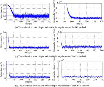
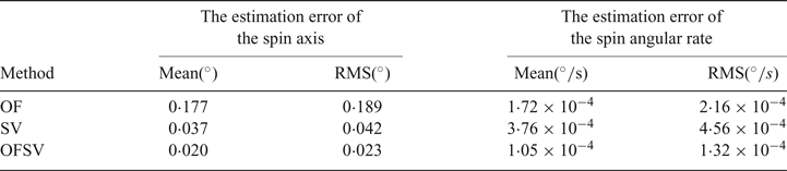
The estimation error of the spin axis (the angle between the estimated spin axis and the real spin axis) and the estimation error of the spin angular rate using three different methods are shown in Figure 1 and Table 1. It can be seen that the estimation of the spin axis using the OF method is worse than using the SV method, while the estimation of the spin angular rate using the OF method is better than using the SV method. The reason is that the directional vector information from the star vector facilitates the determination of the spin axis, while the rate information from optical flow facilitates the estimation of the spin angular rate. The estimation accuracy of the OFSV method using both the spin axis and spin angular rate is the best among the three methods. The convergence rates of the SV method and the OFSV method are better than the OF method. The results demonstrate that the proposed method using optical flow and a star vector as measurement is an attractive choice for attitude estimation of a spinning spacecraft.
The estimation results of three methods.
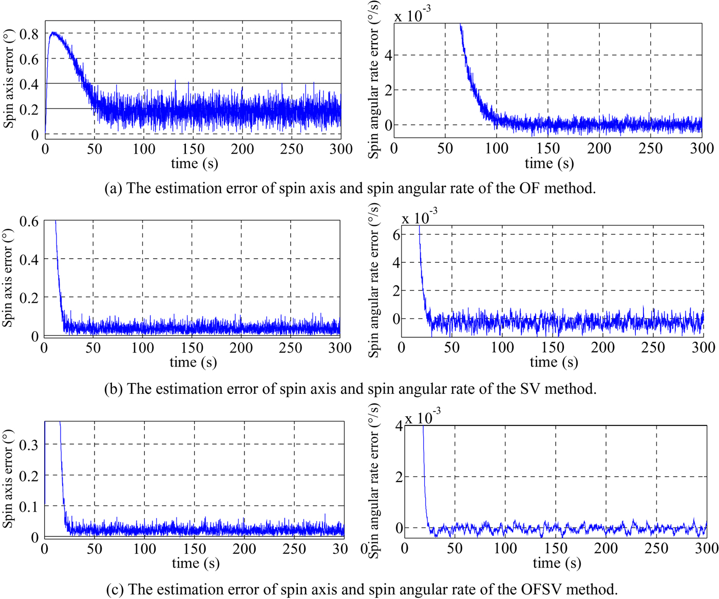
The estimation error of the spin axis and spin angular rate of different methods.

4.2.2. The impact factors of the proposed method using optical flow and a star vector
Some factors which affect the performance of the proposed method are analysed in this section, including spin angular rate, spin axis orientation and spacecraft moment of inertia tensor error.
4.2.2.1. The impact of the spin angular rate
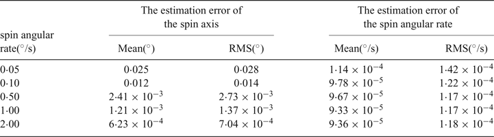
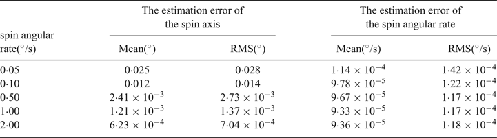
Currently, the dynamic performance of the star sensor can reach 2°/s. Therefore, the spin angular rate discussed here is lower than 2°/s and avoids blurring the star image. The estimation error of the spin axis and the spin angular rate under different spin angular rates is shown in Table 2. From Table 2, it can be seen that the estimation error of the spin axis decreases with the increase of the spin angular rate, while the estimation error of the spin angular rate hardly changes. The reason is that the variation of star coordinates in the sequential star images is at the same level of measurement noise under a small angular rate, which reduces the estimation accuracy of the spin axis.
Estimation error of spin axis and spin angular rate under different spin angular rates.
4.2.2.2. The impact of spin axis orientation
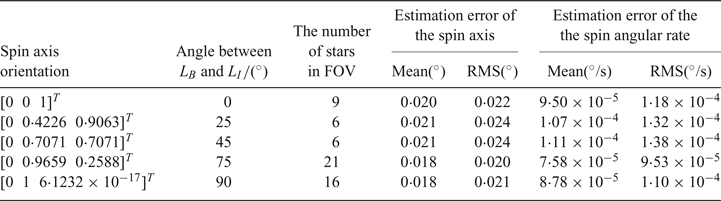
The spin axis orientation of a spacecraft varies due to requirements of different tasks, which leads to different angles between LB and LI. The estimation error of the spin axis and spin angular rate under different spin axis orientations is shown in Table 3. Table 3 also shows the number of stars in the FOV under different spin axis orientation. From Table 3, we can see that the estimation accuracy of the spin axis and the spin angular rate barely varies, as the angle between LB and LI varies from 0° to 90°. The reason for the slight difference in accuracy is that the number of stars in the FOV is different. The more stars in the FOV, the better the estimation accuracy. Therefore, the proposed method has a robust performance in terms of spin axis orientation.
The estimation error of the spin axis and spin angular rate under different spin axis orientations.

4.2.2.3. The impact of spacecraft moment of inertia tensor error
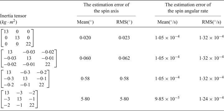
The estimation error of the spin axis and the spin angular rate under different inertia tensors is shown in Table 4. From Table 4, it can be seen that the estimation error of the spin axis increases greatly with the increase in error of the spacecraft moment of inertia tensor, while the estimation error of spin angular rate changes only slightly. This indicates that the proposed method has a robust performance in the estimation of the spin angular rate in terms of inertia tensor error, while the performance in spin axis estimation is seriously affected by inertia tensor error.
The estimation error of the spin axis and spin angular rate under different inertia tensors.

5. CONCLUSIONS
In this paper, a Markley variables-based attitude estimation method using optical flow and a star vector from a star sensor for spinning spacecraft is proposed. Only one star sensor is needed because we can get directional vector information from the star vector and rate information from optical flow, which is equivalent to a combination of a sun sensor, magnetometer and gyro. In addition, the star sensor has a higher accuracy of attitude estimation than the traditional sun sensor and magnetometer, and the star sensor can also replace the gyro in case it is out of action. Simulations reveal that the estimation of the spin axis by the method using only optical flow as the measurement is worse than that of the method only using a star vector as the measurement, while the estimation of the spin angular rate by the method using only optical flow is better than that of the method only using the star vector. The estimation accuracy of both the spin axis and the spin angular rate can be improved by the proposed method using both optical flow and a star vector as the measurements.
ACKNOWLEDGEMENTS
The research presented in this paper has been supported by the National Natural Science Foundation of China (61503013, 61722301) and the grant of the National Basic Research Program of China (973 Program 2014CB744202). The authors wish to express their gratitude to all members of the Science & Technology on Inertial Laboratory, Fundamental Science on Novel Inertial Instrument & Navigation System Technology Laboratory.