Optimization process of the proposed method

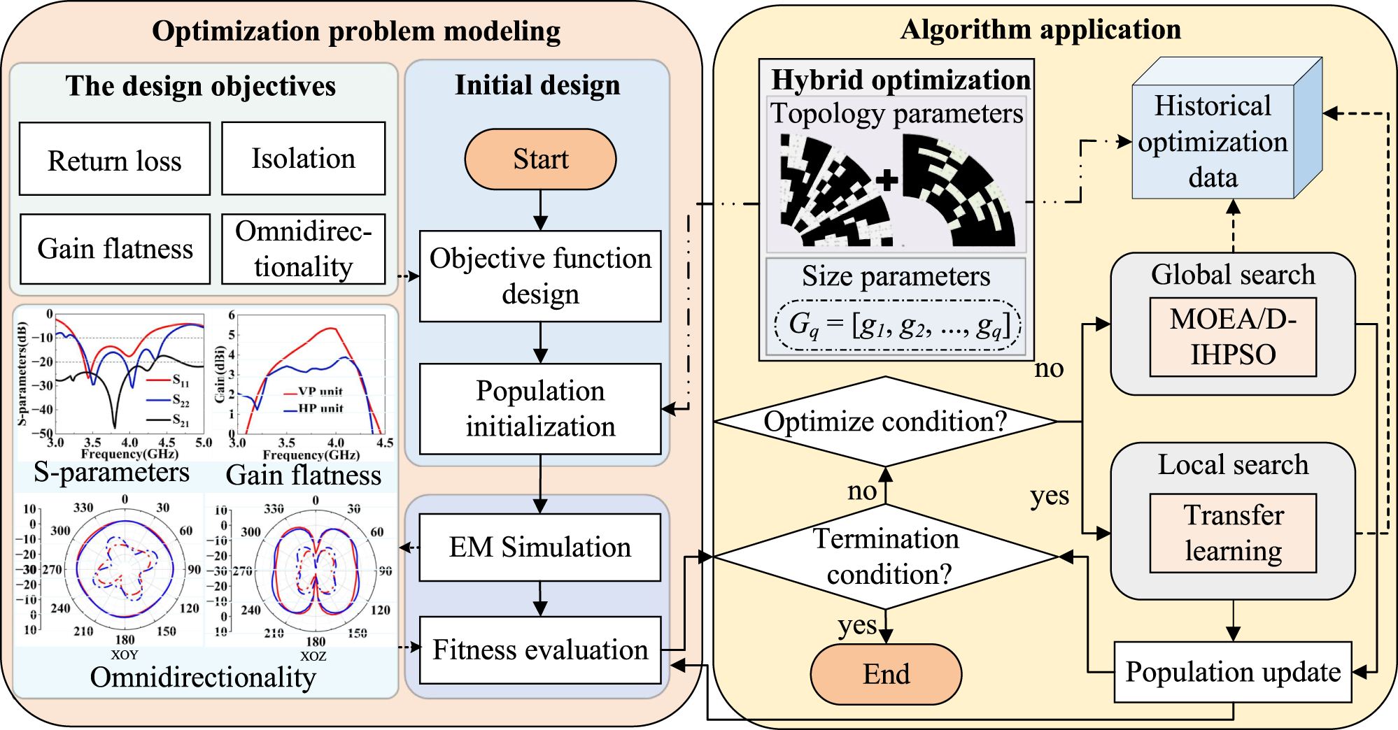
The collaborative optimization framework of the MOEA/D-IHPSO method for efficiently enhancing and balancing multiple performance metrics of the initial antenna design is shown in Fig. 1. First, in the optimization problem modeling phase, a multi-objective function is designed according to the multiple performance index requirements of the antenna. Guided by the surface current distribution as electromagnetic physical prior knowledge, the key regions on the upper and lower radiating patches are selected for optimization. A differentiated network partitioning strategy is used to map the two selected antenna design spaces to binary topology parameter arrays X ₁ = [x ₁, x ₂, …, x_m] and X₂ = [x ₁, x ₂, …, x_n]. At the same time, the key size parameters G_q = [g ₁, g ₂, .., g_q] with the most significant impact on antenna performance are identified using methods such as surface current analysis, equivalent circuit modeling, or sensitivity analysis. The selected topological and size parameters serve as the optimization design variables of the antenna, together forming a hybrid solution vector that establishes a unified search space for concurrent optimization. After defining the population size, Latin Hypercube Sampling [Reference Wu, Chen, Yu, Wang and Hong14] is used to generate the initial population within the defined solution space, laying the foundation for subsequent optimization iterations. Second, in the algorithm application phase, the proposed framework integrates evolutionary and swarm intelligence principles. For the top 50% of individuals in the fitness ranking, a hybrid crossover strategy combining single-point and multi-point crossover is applied to the topology parameters, while simulated binary crossover is used for the size parameters. For the remaining individuals, the improved hybrid particle swarm optimization (IHPSO) guides the updates, wherein an adaptive mutation operator is embedded to dynamically balance global and local search by adjusting the mutation probability according to the fitness convergence status. To further improve search efficiency, a transfer learning-driven recombination strategy is incorporated. It is automatically activated when the convergence rate drops significantly or a specified number of generations is reached, thereby continuously advancing the search for the optimal solution. The optimization process terminates upon reaching the preset iteration limit or meeting multiple preset goals, and the final Pareto optimal solution set is output as the preferred solution for the joint design of antenna topology and size parameters.

Figure 1.

Overall optimization process flow of MOEA/D-IHPSO.

Figure 1 Long description

The flowchart illustrates the optimization process for antenna design using MOEA/D-IHPSO. It is divided into two main sections: Optimization problem modeling and Algorithm application. In the Optimization problem modeling section, the design objectives include return loss, isolation, gain flatness and omnidirectionality. The process begins with the initial design, starting with objective function design, followed by population initialization, EM simulation and fitness evaluation. Graphs are shown for S-parameters, gain flatness and omnidirectionality, with frequency in gigahertz. In the Algorithm application section, hybrid optimization involves topology and size parameters. The process includes checking optimize conditions and termination conditions. If optimization conditions are met, global search using MOEA/D-IHPSO and local search with transfer learning are applied. Historical optimization data is used and population updates occur. The process ends when termination conditions are satisfied.

Objective function design

The design of high-performance antennas requires a rigorous multi-objective optimization framework to simultaneously improve multiple key electromagnetic (EM) performance metrics. The return loss, isolation between the two ports, omnidirectionality, and gain flatness are used as optimization objectives in this paper. The optimization problem is transformed into the following mathematical expression to guide the algorithm in fully exploring the optimal performance of the antenna.

(1)\begin{equation}\begin{gathered} \mathop {\min }\limits_Z F(Z) = ({f_1}(Z),{f_2}(Z),{f_3}(Z),{f_4}(Z),{f_5}(Z)) \hfill \\ \qquad\qquad\quad\quad{\text{ }}s.t.{\text{ }}Z \in \Omega \hfill \\ \end{gathered} \end{equation}

The variable Z is the decision variable of the topology parameters X and the size parameters G_q, while Ω denotes the design space. For ports 1 and 2, to ensure that the return loss is greater than C ₁ (dB) within the operating frequency band [ω ₁, ω ₂], the objective functions f ₁(Z) and f ₂(Z) are defined as follows.

(2)\begin{equation}{f_i}(Z) = \max ({C_1} - \mathop {\min }\limits_{\omega \in \left[ {{\omega _1},{\omega _2}} \right]} \left| {{S_{ii}}(Z,\omega )} \right|,0) \cdot (1 + \gamma ){\text{ }}\end{equation}

i = 1 and 2. In order to suppress mutual coupling between the two ports and ensure that the isolation of the optimized antenna is higher than C ₂ (dB), the objective function f ₃(Z) is defined as follows.

(3)\begin{equation}{f_3}(Z) = \max ({C_2} - \mathop {\min }\limits_{\omega \in \left[ {{\omega _1},{\omega _2}} \right]} \left| {{S_{21}}(Z,\omega )} \right|,0) \cdot (1 + \gamma )\end{equation}

γ is the penalty factor. Within the operating frequency range, when min|S_ii| is below C ₁ dB or min|S ₂₁| is below C ₂ dB, the penalty value is linearly proportional to the exceeding amplitude. Additionally, to ensure that the optimized antenna has satisfactory omnidirectional radiation characteristics at multiple key frequency points, the omnidirectional fluctuation objective function f ₄(Z) is defined as follows.

(4)\begin{equation}\begin{gathered} \qquad\qquad\quad\quad\quad{\text{ }}{f_4}(Z) = \max ({f_4}(Z){|_{{f_1}}},{f_4}(Z){|_{{f_2}}}) \hfill \\ {f_4}(Z){|_{{f_i}}} = \max ([\mathop {\max }\limits_\varphi G(Z,{f_i},\varphi ,{\theta _0}) - \mathop {\min }\limits_\varphi G(Z,{f_i},\varphi ,{\theta _0})] - {C_3},0) \hfill \\ \end{gathered} \end{equation}

G(Z, f_i, φ, θ ₀) represents the realized gain evaluated at frequency f_i, azimuth angle φ, and a fixed elevation angle θ ₀, while C ₃ denotes the threshold for omnidirectional performance. To further improve the performance stability of the antenna within the operating frequency band and suppress fluctuations in the gain-frequency response curve, the gain-flatness objective f ₅(Z) is defined as follows.

(5)\begin{equation}{f_5}(Z) = \max ([\mathop {\max }\limits_{\omega \in \left[ {{\omega _1},{\omega _2}} \right]} G(Z,\omega ) - \mathop {\min }\limits_{\omega \in \left[ {{\omega _1},{\omega _2}} \right]} G(Z,\omega )] - {C_4},0)\end{equation}

G(Z,ω) represents the realized gain within the operating frequency band. C ₄ is the threshold for the gain flatness level. A smaller f ₅(Z) indicates a more stable antenna gain.

For an antenna to operate in a frequency band ranging from 3.3 to 4.1 GHz, the objective function is specified by setting (ω ₁, ω ₂) = (3.3 GHz, 4.1 GHz) and (C ₁, C ₂) = (10 dB, 20 dB), so that the optimized antenna attains a return loss better than 10 dB and an isolation better than 20 dB. As a gain variation of less than 3 dB is widely recognized as indicative of excellent omnidirectional performance and stable gain [Reference Yan, Zhai, Ren and Zhang22, Reference Feng, Li, Chung, Sim and Deng23], C ₃ and C ₄ are set to 3 dB to ensure that the antenna design meets this standard. Furthermore, to guarantee the performance at key frequencies within the band, f ₁ and f ₂ are set to 3.5 and 3.8 GHz, respectively. The optimization range for the key size parameter h is set to 5–10 mm, which is determined by combining theoretical considerations of the coupling length [Reference Wu, Yang, Chen, Qu and Nie24] with systematic parametric sweep results. R ₇ is set to 1–4 mm to ensure mechanical compatibility with standard metric screws for manufacturability.

Topology optimization region division strategy based on current distribution characteristics

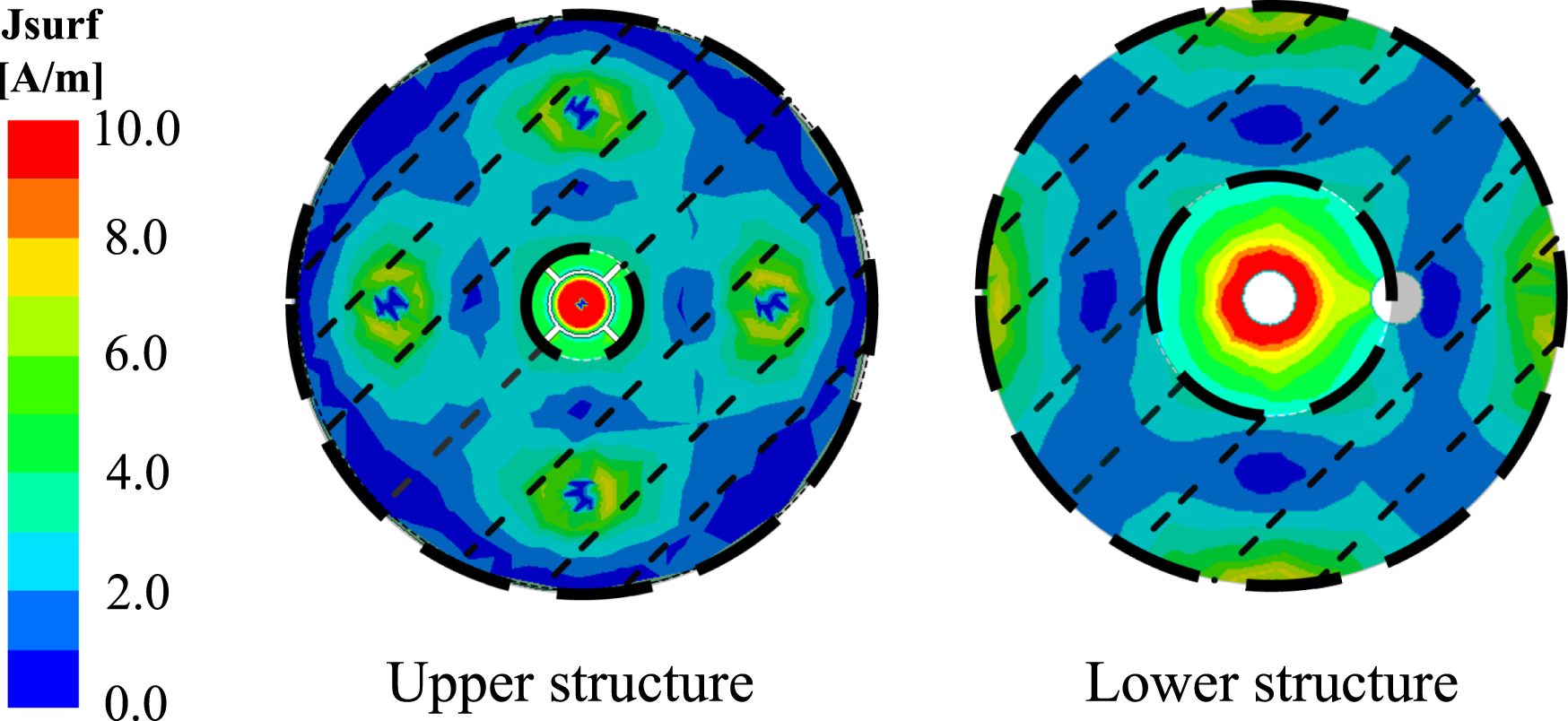
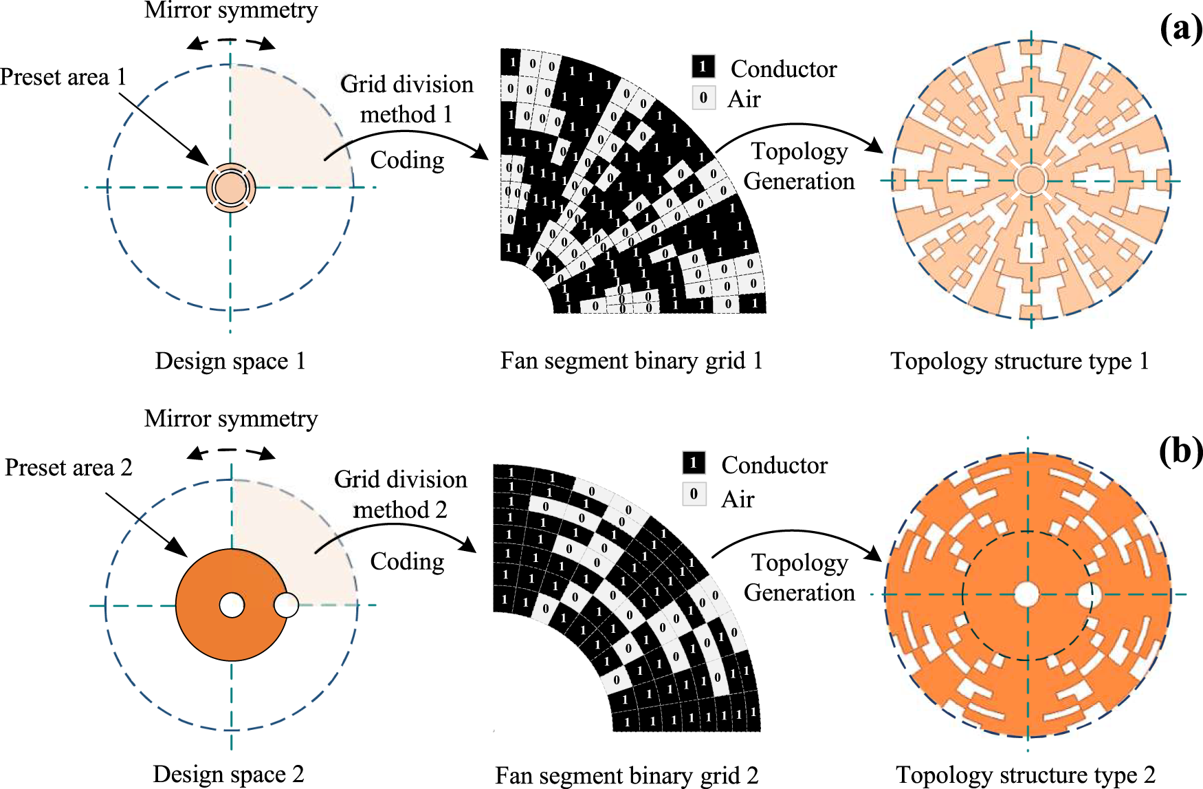
Based on the lightweight and easily integrable nature of planar fragmented structures (FTS), the MOEA/D-IHPSO algorithm is employed to search for the optimal topological distribution of FTS within the refined unit design space. According to the surface current distributions on the upper and lower radiating patches, regions with significant current-intensity variation are selected for optimization. Meanwhile, to avoid geometric defects introduced by sector discretization, a circular patch is preset in the design. The selected optimization region is shown as the shaded area in Fig. 2. To further implement the structured grid division, the selected region is divided into four equal sectors by two perpendicular dashed lines passing through the circle center, as shown in Fig. 3. One sector is discretized into sector-ring unit cells in polar coordinates and mapped onto the binary design matrix. “1” represents a metal unit cell and “0” represents a non-metal unit cell. This novel physics-informed binary encoding interface is crucial for balancing design accuracy and optimization efficiency, while reducing error accumulation. Finally, the complete radiation patch is obtained by mirroring and rotating operations to ensure structural symmetry, which is fundamental for achieving the desired omnidirectional radiation pattern.

Figure 2.

Current distribution and optimization region.

Figure 2 Long description

A vertical scale bar is shown with the label “Jsurf” and “[A/m]”. Tick labels on the scale read 10.0, 8.0, 6.0, 4.0, 2.0 and 0.0. The scale indicates Jsurf magnitude, with 0.0 at the bottom of the scale and 10.0 at the top of the scale. The heatmap titled “Upper structure” shows a circular field with a small central circular area enclosed by two thin concentric circles. The highest Jsurf values appear at the center as a compact region near the top end of the scale. Additional localized higher-value regions appear away from the center at several separated positions around the disk. Lower-value regions occupy much of the remaining area between these localized regions. The heatmap titled “Lower structure” shows a circular field with a central ring-shaped region around a small circular center. The highest Jsurf values form a ring near the center, corresponding to the top end of the scale. Outside the central ring, most areas show lower values, with a few localized mid-to-higher regions nearer the outer part of the disk. Across the two heatmaps, the “Upper structure” concentrates the strongest values in a small central spot plus multiple off-center localized regions, while the “Lower structure” concentrates the strongest values in a central ring with fewer separated off-center regions.

Figure 3.

Two network partitioning strategies and binary encoding of topological structures. (a) Non-uniform angular partitioning network and (b) equal area sector partitioning network.

Figure 3 Long description

The image consists of two parts labeled as (a) and (b), each illustrating a different network partitioning strategy with binary encoding for topological structures. In part (a), the design space 1 is shown with a circular area labeled 'Preset area 1' and divided by dashed lines indicating mirror symmetry. The grid division method 1 is applied, leading to a fan segment binary grid 1, where '1' represents a conductor and '0' represents air. This grid is used for topology generation, resulting in topology structure type 1, which maintains the mirror symmetry. In part (b), design space 2 is depicted with 'Preset area 2', also divided by dashed lines for mirror symmetry. Grid division method 2 is applied, producing fan segment binary grid 2 with the same binary coding for conductors and air. This leads to topology structure type 2, which also exhibits mirror symmetry. Both parts emphasize the process of coding and topology generation from the initial design spaces to the final topological structures.

After selecting the optimization region, two efficient mesh division strategies are proposed based on the current-distribution characteristics of the selected area (Fig. 2) to further enhance design flexibility. The current in the upper structure shows a distinct edge accumulation characteristic, so a non-uniform angular partitioning strategy is applied to this region. Specifically, the sectorial optimization region is evenly divided into 8 annular layers to balance modeling accuracy and the number of optimization variables. The angular direction is divided into 10 equal parts near the axis, while the edge region where the current intensity changes more significantly is divided into 20 equal parts to achieve refined optimization of the key areas, as shown in Fig. 3(a). The current distribution in the lower structure is more uniform, so an equal-area meshing strategy is adopted, as shown in Fig. 3(b). In this approach, the angular direction is divided into 10 equal parts, and the radial direction is partitioned into 8 layers with proportionally scaled boundaries to ensure that each sector ring unit has an equal area. This results in a moderately sized 8 × 10 grid that balances optimization across the region and enhances manufacturability. The combination of these two strategies not only helps suppress the accumulation of discrete errors in topology optimization, but also ensures design accuracy and practical feasibility during the optimization process, thereby improving the overall optimization effect.

Improved HPSO

To address the joint optimization problem of topology and size parameters, this study proposes an IHPSO algorithm. This algorithm combines BPSO and continuous particle swarm optimization for the joint optimization of discrete topology parameters and continuous size parameters within a unified coding framework. A mixed encoding scheme is employed for each particle, in which the topology parameters are represented by 0/1 Boolean variables representing fragmented metal structures, and the size parameters are encoded as real numbers. After each update, the size parameters are rounded to one decimal place to satisfy manufacturing tolerance requirements. The topology parameters are updated using the sigmoid function in BPSO for probabilistic flipping, and the mapping function is given as follows.

(6)\begin{equation}S({v_k}) = \frac{1}{{1 + {e^{ - v}}}}\end{equation}

v represents the velocity value of the current position of the particle, which is used to control the probability of topological site flipping.

Meanwhile, IHPSO introduces an adaptive mutation mechanism based on fitness to enhance population diversity and prevent premature convergence. The mutation probability P is dynamically adjusted according to the difference between the average aggregate fitness f _av of a few elite individuals in the previous generation and the fitness threshold f _th.

(7)\begin{equation}P = \left\{ {\begin{array}{*{20}{l}} {{P_{{\text{max}}}},}&{{f_{{\text{av}}}} \lt {f_{{\text{th}}}}} \\ {{P_{{\text{min}}}} + ({P_{{\text{max}}}} - {P_{{\text{min}}}}) \cdot (1 - \frac{{{f_{av}} - {f_{th}}}}{{{f_{av}}}}),}&{{f_{{\text{av}}}} \geqslant {f_{{\text{th}}}}} \end{array}} \right.\end{equation}

The mutation probability P is dynamically adjusted within a preset range [P _min, P _max]. If f_av falls below the threshold f _th, the mutation rate P is increased to enhance population diversity. After the mutation is triggered, the topological parameters and size parameters are differentially perturbed. The topological parameters undergo a Boolean flip operation on their elements with probability P. The size parameters are perturbed by adding a standard normal random term to the current position, thereby helping the search escape local optima in the continuous space. The improved operator dynamically adjusts the mutation strength according to the current search state, thus better balancing global search and local optimization and preventing the algorithm from getting stuck in local optima.

Transfer learning-driven recombination strategy

To further enhance the efficiency of automated antenna design, a transfer learning-driven joint recombination strategy for topology and size parameters is proposed. The transfer learning mechanism adopted by this strategy is different from the typical deep learning paradigm. It does not rely on model training, but instead achieves knowledge transfer and reuse by directly reorganizing and perturbing structural modules and parameters extracted from high-performing individuals in historical optimization runs. This mechanism aims to improve the quality and diversity of the population. The detailed procedure is as follows.

In the first step of the process, the fitness improvement rate ΔF ^(g) is defined to monitor the evolutionary trend of the population.

(8)\begin{equation}\Delta {F^{(g)}} = \frac{{F_{best}^{(g)} - F_{best}^{(g - 1)}}}{{|F_{best}^{(g - 1)}| + \varepsilon }}\end{equation}

F ^(g)_best represents the optimal total fitness of the gth generation and ε is a small positive number set to 1 × 10⁻¹⁰ to ensure numerical stability. The transfer learning-driven recombination strategy is triggered when the algorithm detects convergence stagnation. Specifically, stagnation is identified if the fitness improvement rate remains below a predefined threshold for a specified number of consecutive generations.

(9)\begin{equation}\frac{1}{T}\sum\limits_{k = 1}^T \Delta {F^{(g - k)}} \lt \delta ,\quad g \gt T\end{equation}

δ is the fitness improvement threshold and is set to 0.01 based on observations of the initial algorithm convergence rate. T is the number of consecutive stagnant generations and is empirically set to 5 to ensure reliable detection. Subsequently, the system selects the top N individuals (N is the current population size) from the historical optimization data based on the five indicators S ₁₁, S ₂₂, S ₂₁, omnidirectionality, and gain flatness, respectively, to construct five distinct label pools T ₁₁, T ₂₂, T ₂₁, T_o, and T_g. After the structural label is constructed, the individuals in the population can be expressed as follows.

(10)\begin{equation}{I^{(i)}} = \left\{ {B_1^{(i)},B_2^{(i)},\ldots,B_n^{(i)},{G_q}^{(i)}} \right\}\end{equation}

B_j ⁽ⁱ⁾ represents the jth layer structure module in the ith individual topology structure. G_q ⁽ⁱ⁾ is the vector of q parameters associated with the individual I ⁽ⁱ⁾.

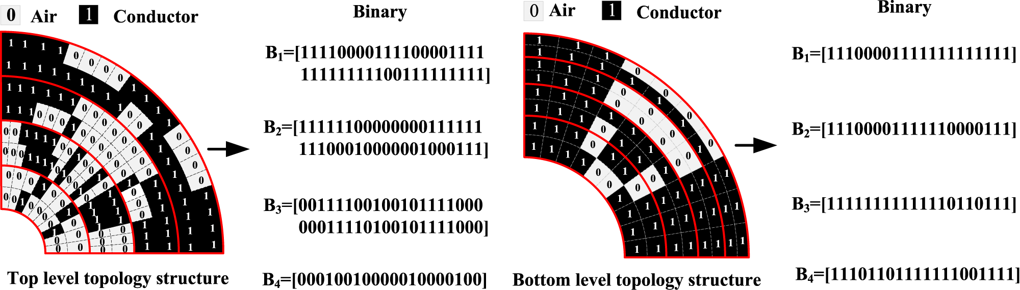
The strategy then performs splicing and recombination of the topological structures. The individuals in the label pool are uniformly divided into four structural modules (Fig. 4), forming four corresponding module pools. The strategy randomly selects one module from each module pool with equal probability and splices them into a new structural individual. If a module pool contains M modules, the probability of selecting any specific module from it is 1/M.

(11)\begin{equation}{B_{new}} = [{B_1}^{(p)},{B_2}^{(q)},{B_3}^{(r)},{B_4}^{(s)}]\end{equation}

p, q, r, and s are the indices for the four randomly selected modules.

Figure 4.

Schematic diagram of topology structure modularity.

Figure 4 Long description

The image consists of two semicircular diagrams labeled as top level topology structure and bottom level topology structure. Both diagrams are divided into concentric segments, each containing smaller sections marked with binary digits zero and one. The binary digit zero represents air, while one represents conductor, as indicated by the labels at the top of the image. In the top level topology structure, the segments are arranged in a pattern with alternating zeros and ones, forming a complex design. An arrow points from this structure to a set of binary sequences labeled B subscript 1, B subscript 2, B subscript 3 and B subscript 4. Each sequence is enclosed in square brackets and represents the binary configuration of the corresponding segment. The bottom level topology structure follows a similar pattern but with a different arrangement of zeros and ones. An arrow from this structure also points to a set of binary sequences labeled B subscript 1, B subscript 2, B subscript 3 and B subscript 4, each enclosed in square brackets. These sequences represent the binary configuration of the segments in the bottom level topology structure. The binary sequences are displayed to the right of each semicircular diagram, illustrating the conversion of the visual topology into binary form.

Finally, parameter perturbation sampling is conducted to generate the size parameters for the newly recombined topology. The system first identifies the set S of all historical elite individuals that contribute modules to B _new. A new size parameter vector G _new is then generated by applying a Gaussian perturbation to the mean parameters according to the following formula.

(12)\begin{equation}{G_{new\,}}\, = \,\frac{1}{{\left| S \right|}}\sum\limits_{{I^{(i)}} \in S} {G_q^{(i)}\, + \,\eta \cdot \epsilon } ,\, \epsilon \, \in \,{\text{N(0,}}{\sigma ^2}{\text{I)}}\,\end{equation}

η is the perturbation coefficient, typically set to 0.1 to control the overall scale of exploration. The vector ϵ is a multivariate Gaussian noise, where σ ² defines its variance, usually set to a small fraction of the allowable parameter range. The identity matrix I ensures that the noise is added independently to each size parameter with equal variance. All generated parameter values are constrained to the feasible manufacturing range. This approach performs directed perturbation based on excellent parameter benchmarks, effectively utilizing historical experience while ensuring the diversity of the new parameters. The new topology B _new and its associated parameters G _new are concatenated to form a new candidate individual I _new = [B _new, G _new]. This process is repeated to generate the new population.

This strategy significantly enhances the directionality and diversity of the structural reconstruction process by integrating the triple mechanisms of structural label guidance, module reorganization, and parameter reorganization sampling, thereby effectively improving the overall convergence efficiency. This improvement is achieved with negligible computational overhead.

Introduction of the initial and optimized antenna structure

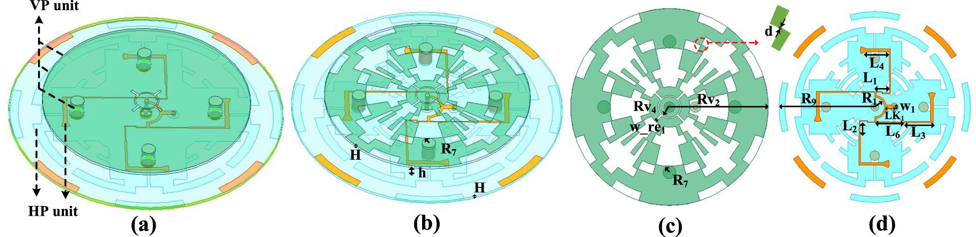
To verify the effectiveness of the proposed MOEA/D-IHPSO for antenna optimization, a dual-polarized omnidirectional antenna is optimized. The antenna structure consists of a vertical polarization (VP) unit and a horizontal polarization (HP) unit, and its initial configuration is shown in Fig. 5(a), which employs an FR-4 substrate with a relative permittivity of 4.4 and a loss tangent of 0.02. The optimized antenna configuration is shown in Fig. 5(b), with the optimal topological layouts of the upper and lower antenna layers presented in Fig. 5(c) and (d). The optimal values of h and R ₇ are 6 and 2.5 mm, respectively. To ensure overall electrical continuity of the segmented structure, the edge length of each unit increases successively by 0.15 mm along the radial direction.

Figure 5.

Initial and optimized structure of the dual-polarized omnidirectional antenna. H = 1, h = 6, R ₁ = 6, R ₇ = 2.5, R ₉ = 49.5, Rv₂ = 38, Rv₄ = 4.5, w_re₁ = 0.4, L ₁ = 8, L ₂ = 7.2, L ₃ = 15, L ₄ = 12, L ₆ = 15.2, LK₁ = 6, W ₁ = 2, d = 0.15 (units: mm). (a) Initial structure, (b) optimized structure, (c) optimized upper layer, and (d) optimized lower layer.

Figure 5 Long description

The diagram illustrates the design evolution of a dual-polarized omnidirectional antenna across four sub-images. The first sub-image (a) displays the initial structure, highlighting the vertical polarization unit at the top and the horizontal polarization unit at the bottom. This layout employs an FR-4 substrate. The second sub-image (b) shows the optimized structure, where dimensions such as H equals 1 millimeter, h equals 6 millimeters and R7 equals 2.5 millimeters are indicated. The third sub-image (c) presents the optimized upper layer, featuring components labeled Rv4, Rv2, w_re and R7, with a directional arrow indicating a distance labeled d equals 0.15 millimeters. The fourth sub-image (d) depicts the optimized lower layer, showing various labeled elements including E4, L1, L2, L3, L4, L5, L6, LK, W1 and R9, arranged in a circular pattern with connections between them. These diagrams represent top-view layout drawings of the antenna's geometry, illustrating the transition from initial to optimized design to improve performance. The optimization focuses on enhancing the antenna's electrical continuity and polarization capabilities, with specific measurements provided for clarity and precision.

Experimental environment and optimization results

The entire simulation process is performed on a computer equipped with 128 GB of memory, an Intel Core i9–14900KS processor, and an NVIDIA GeForce RTX 5060 GPU. The simulation software is ANSYS HFSS 2022R1. To enable automated simulation, the binary-encoded topology matrix generated by the algorithm is programmatically converted into a standard CAD file, which is then imported into HFSS for full-wave electromagnetic analysis and performance evaluation. The optimized areas of the sector-shaped radiating patches on the upper and lower layers are discretized into 140 and 8 × 10 units. In MOEA/D-IHPSO, the initial population size N is set to 36 and the maximum number of iterations N_t is set to 50.

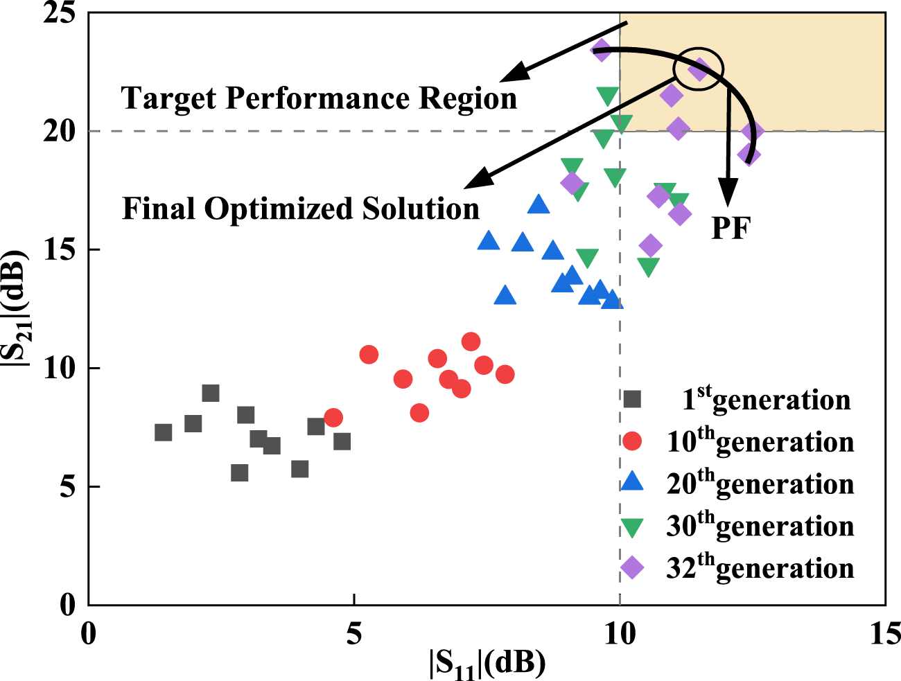
After 32 iterations of optimization, which correspond to 1152 full-wave solutions, the topology configuration of both design spaces and the size parameters h and R ₇ are simultaneously converged. The bandwidth optimized by MOEA/D-IHPSO is from 3.27 to 4.2 GHz, with isolation above 20 dB across this frequency band. Moreover, the gain curve exhibits a smooth variation, and at the frequency points of 3.5 and 3.8 GHz, the gain fluctuation in the azimuth plane is less than 3 dB, which verifies the engineering feasibility of simultaneously optimizing both the topology and size parameters. The evolution trajectory of some representative solutions from the Pareto set is shown in Fig. 6. With optimization iterations, the solution population evolves from an initial random distribution to a high concentration in the target performance region. The majority of solutions in the final generation converge to the Pareto front, demonstrating the effective trade-off of the algorithm between reflection loss and isolation.

Figure 6.

Pareto frontier solution and optimization process evolution.

Figure 6 Long description

The horizontal axis label is vertical bar S subscript 11 vertical bar (dB). The horizontal axis shows tick labels 0, 5, 10, 15. The vertical axis label is vertical bar S subscript 21 vertical bar (dB). The vertical axis shows tick labels 0, 5, 10, 15, 20, 25. Text inside the plot reads “Target Performance Region” and “Final Optimized Solution”. The label “PF” appears near the upper right area with arrows pointing toward a circled point. A dashed vertical line is drawn at 10 on the horizontal axis. A dashed horizontal line is drawn at 20 on the vertical axis. A legend lists five categories with marker shapes: “1st generation” shown with square markers, “10th generation” shown with circle markers, “20th generation” shown with upward triangle markers, “30th generation” shown with downward triangle markers and “32th generation” shown with diamond markers. The square markers are clustered around horizontal axis values roughly from 1 to 5 and vertical axis values roughly from 5 to 9. The circle markers are clustered around horizontal axis values roughly from 5 to 8 and vertical axis values roughly from 8 to 11. The upward triangle markers are clustered around horizontal axis values roughly from 7 to 10 and vertical axis values roughly from 12 to 17. The downward triangle markers are clustered around horizontal axis values roughly from 9 to 11 and vertical axis values roughly from 14 to 21. The diamond markers are clustered around horizontal axis values roughly from 10 to 13 and vertical axis values roughly from 15 to 24.

The proposed MOEA/D-IHPSO can be extended to other planar antenna designs, such as microstrip patch antennas and planar monopole antennas, where discrete topology patterns and continuous geometric parameters need to be optimized simultaneously for multiple performance objectives. In practice, the overall computational expense is still dominated by full-wave simulations, while the added cost of the evolutionary operators and transfer learning-driven recombination remains lightweight. Although the initial population is generated stochastically, sensitivity to initialization is mitigated by IHPSO and a recombination mechanism that injects high-quality modules from historical data.

The measurement results of antenna

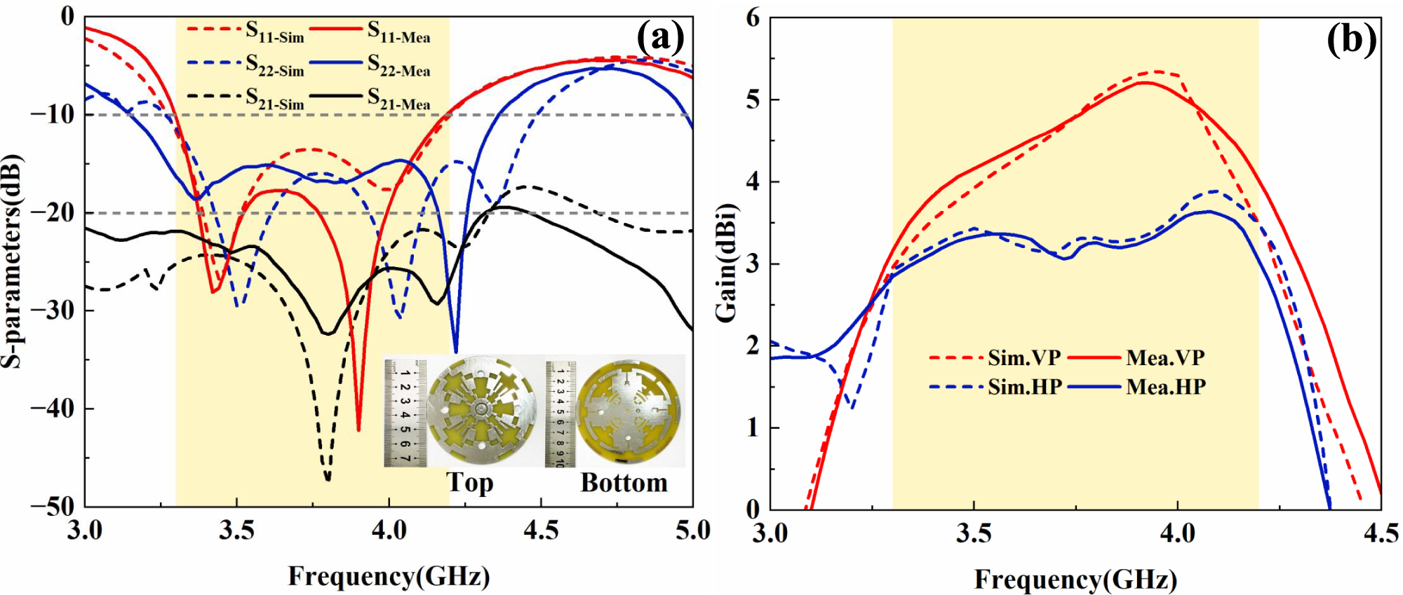
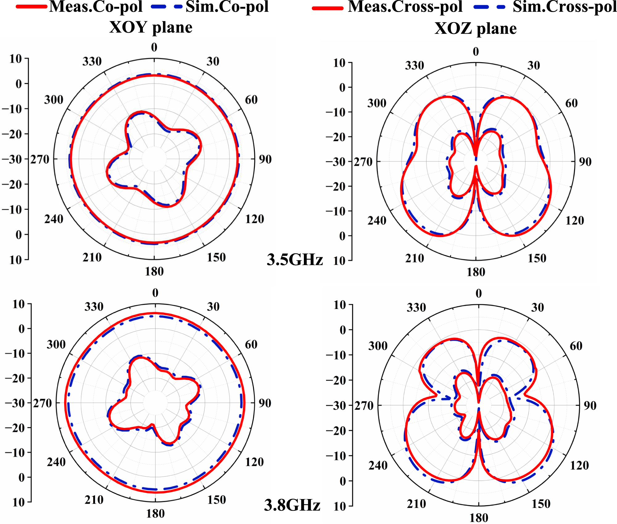
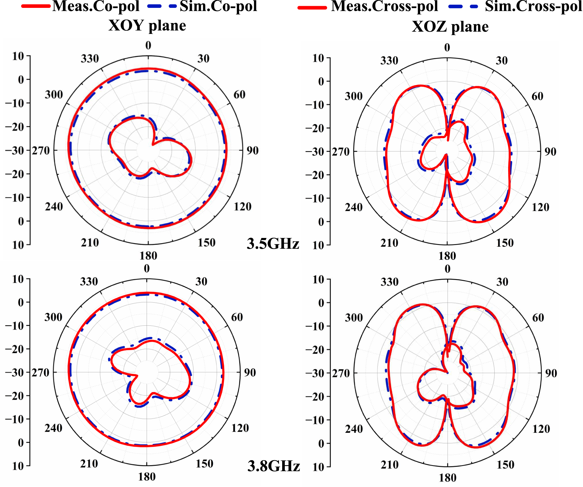
To verify the engineering effectiveness and optimization performance of the MOEA/D-IHPSO algorithm, the optimized dual-polarized omnidirectional antenna is experimentally tested. As shown in Fig. 7(a), the measured −10 dB impedance bandwidth is from 3.3 to 4.2 GHz. The peak gain values of the VP and HP units are shown in Fig. 7(b), with VP varying between 3.16 and 5.21 dBi, and HP varying between 2.85 and 3.64 dBi. The radiation patterns of the designed antenna at several frequencies are shown in Figs. 8 and 9. The gain variation on the XOY plane is less than 1.8 dB, and the gain pattern on this plane demonstrates good omnidirectional characteristics. In addition, a low cross-polarization level of the two polarizations can be observed, which is less than −15 dB. The measured and simulated results are generally consistent. The discrepancy between the measured and simulated values may be attributed to manufacturing tolerances, welding deviations, and non-ideal measurement environments.

Figure 7.

The simulated and measured results of the optimized antenna. (a) S-parameters and (b) peak gain.

Figure 7 Long description

The image A showing a line graph labeled (a). The y-axis label is “S-parameters(dB)”. The y-axis ranges from 0 to minus 50 with labeled ticks at 0, minus 10, minus 20, minus 30, minus 40 and minus 50. The x-axis label is “Frequency(GHz)”. The x-axis ranges from 3.0 to 5.0 with labeled ticks at 3.0, 3.5, 4.0, 4.5 and 5.0. A horizontal dashed reference line is drawn at minus 10. The legend lists six curves: S subscript 11 Sim, S subscript 11 Mea, S subscript 22 Sim, S subscript 22 Mea, S subscript 21 Sim and S subscript 21 Mea. The plotted curves show multiple minima between about 3.3 and 4.3 on the frequency axis, with several curves dropping below minus 20 and some dropping below minus 40. An inset at the lower right contains two small circular device photos labeled “Top” and “Bottom”, each shown next to a ruler. The image B showing a line graph labeled (b). The y-axis label is “Gain(dBi)”. The y-axis ranges from 0 to 6 with labeled ticks at 0, 1, 2, 3, 4, 5 and 6. The x-axis label is “Frequency(GHz)”. The x-axis ranges from 3.0 to 4.5 with labeled ticks at 3.0, 3.5, 4.0 and 4.5. The legend lists four curves: Sim.VP, Mea.VP, Sim.HP and Mea.HP. The VP curves rise from near 0 around 3.0 to above 5 near about 4.0, then fall toward 0 by about 4.5. The HP curves rise from about 2 near 3.0 to around the mid 3 range near about 4.0, then fall toward 0 by about 4.5.

Figure 8.

Measured and simulated gain patterns for the VP element at 3.5 and 3.8 GHz.

Figure 8 Long description

Four polar plots show measured and simulated gain patterns for co-polar and cross-polar configurations at 3.5 gigahertz and 3.8 gigahertz. The XOY and XOZ planes are depicted. The radial axis represents gain in decibels, ranging from -30 to 10. The angular axis covers 0 to 360 degrees. Solid red lines indicate measured co-polar and cross-polar gains, while dashed blue lines represent simulated gains. At 3.5 gigahertz, the XOY plane shows a multi-lobed pattern with peaks near 0, 90, 180 and 270 degrees. The XOZ plane displays a figure-eight shape with peaks around 0 and 180 degrees. At 3.8 gigahertz, similar patterns are observed with slight variations in peak and null positions. The measured and simulated patterns closely overlap, with minor discrepancies in specific angles, indicating good agreement between the two sets of data.

Figure 9.

Measured and simulated gain patterns for the HP element at 3.5 and 3.8 GHz.

Figure 9 Long description

The image contains four polar plots illustrating measured and simulated gain patterns for co-polar and cross-polar configurations at 3.5 GHz and 3.8 GHz. The XOY plane plots show co-polar patterns, while the XOZ plane plots show cross-polar patterns. The radial axis likely represents gain in decibels, with tick marks at 10, 0, minus 10, minus 20 and minus 30. The angular scale is marked in degrees from 0 to 360. At 3.5 GHz, the XOY plane plot shows measured and simulated co-polar patterns with outer traces near 0 to 10 dB and inner multi-lobed traces around minus 20 to minus 30 dB, with lobes oriented toward 60 to 120 degrees and 240 to 300 degrees. The XOZ plane plot shows cross-polar patterns with large lobes near 0 and 180 degrees reaching near 0 dB and narrower regions near 90 and 270 degrees closer to minus 20 to minus 30 dB. At 3.8 GHz, the XOY plane plot shows similar co-polar patterns with outer traces near 0 to 10 dB and inner multi-lobed traces around minus 20 to minus 30 dB, with broader lobes around 60 to 120 degrees and smaller lobes around 210 to 270 degrees. The XOZ plane plot shows cross-polar patterns with large lobes near 0 and 180 degrees close to 0 dB, with reduced radius near 90 and 270 degrees toward minus 20 to minus 30 dB. Overall, the measured and simulated patterns closely match, with small deviations near nulls. The patterns demonstrate consistent multi-lobe shapes across both frequencies, with minor differences in lobe orientation and depth.

Comparison of the proposed method with other methods

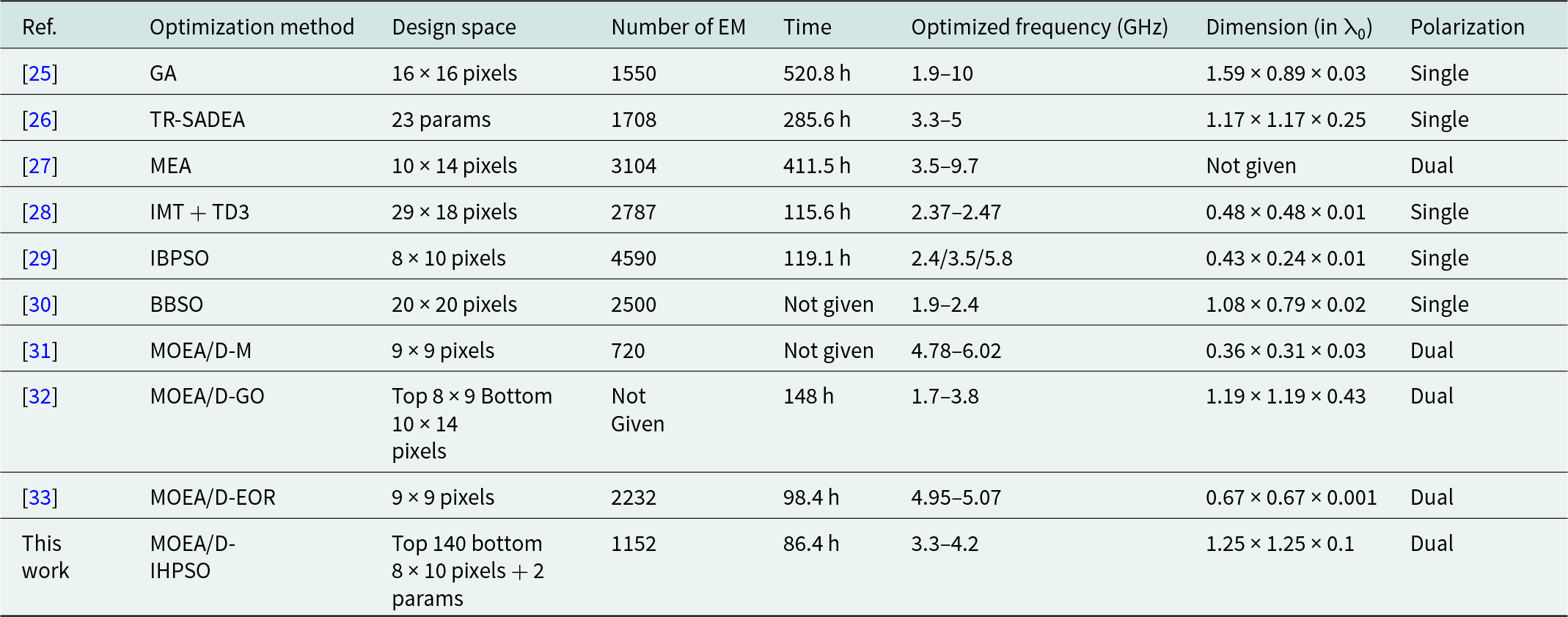
Table 1 summarizes the key performance indicators of the proposed algorithm and several multi-objective evolutionary algorithms from the literature. Compared with the traditional genetic algorithm-based approach [Reference John and Ammann25], surrogate model-assisted methods [Reference Liu, Akinsolu, Song, Hua, Excell, Xu and Huang26, Reference Huang, Yang and Wang27] and image mapping topology with twin delayed deep deterministic policy gradient (IMT + TD3) method [Reference Dou, Gong, Chen, Chen, Shen and Song28], this method shows better performance in terms of optimization speed and convergence, especially in high-dimensional and multi-objective problems, avoiding the problem of easily falling into local optimality. Compared with the IBPSO and BBSO methods [Reference Dong, Li and Deng29, Reference Aldhafeeri and Rahmat-Samii30], the proposed optimization framework can better cope with the nonlinear relationship between topology and size parameters when dealing with complex antenna structures, thereby achieving more accurate design optimization. Compared with the multi-objective evolutionary algorithm-based methods [Reference Li, Chu and Chang31–Reference Wang, Wang, Wang and Zhang33], MOEA/D-IHPSO can better handle mixed optimization problems of discrete and continuous variables, provide a more flexible optimization space in antenna design, and maintain good global search capabilities while achieving efficient optimization.

Table 1.

Comparison information with similar optimization algorithms

Table 1 Long description

The table compares multiple antenna/structure optimization approaches by design-space size, number of electromagnetic (EM) simulations, total optimization time, achieved operating frequency range, normalized physical dimensions (in units of λ0), and polarization. “This work” (MOEA/D–IHPSO) reports 1152 EM runs and the shortest stated runtime, 86.4 h, producing dual polarization over 3.3–4.2 GHz with size 1.25×1.25×0.1 λ0. Other methods with reported times are slower: MOEA/D–EOR 98.4 h (2232 EM, dual, 4.95–5.07 GHz), MOEA/D–GO 148 h (EM not given, dual, 1.7–3.8 GHz), IMT+TD3 115.6 h (2787 EM, single, 2.37–2.47 GHz), IBPSO 119.1 h (4590 EM, single, 2.4/3.5/5.8 GHz), TR–SADEA 285.6 h (1708 EM, single, 3.3–5 GHz), MEA 411.5 h (3104 EM, dual, 3.5–9.7 GHz; size not given), and GA 520.8 h (1550 EM, single, 1.9–10 GHz). Two entries omit time (BBSO and MOEA/D–M), and one omits EM count (MOEA/D–GO), limiting full efficiency comparisons across all rows. Dual-polarized designs appear in MEA, MOEA/D–M, MOEA/D–GO, MOEA/D–EOR, and this work, while most others are single-polarized. Frequency coverage varies widely, from narrow bands near 2.4 GHz (IMT+TD3) or 5 GHz (MOEA/D–EOR) to broad ranges such as 1.9–10 GHz (GA), so runtime and EM counts should be interpreted alongside differing bandwidth targets and design-space complexity.

Note: λ₀ is the wavelength at the center frequency of the operation band.

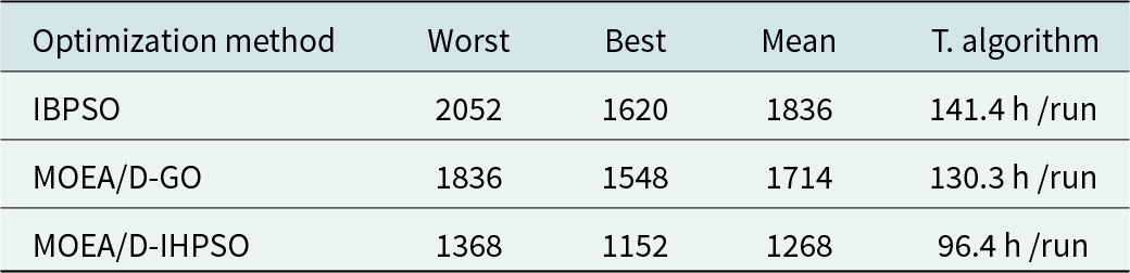
The mean number of EM simulations and time consumption under 5 independent runs for different algorithms are presented in Table 2. The number of EM simulations for MOEA/D under the worst, best, and mean optimization efficiency is 1368, 1152, and 1268, respectively. Based on the average time over 5 runs, the optimization efficiency of this framework (96.4 hours) is improved by 31.8% and 26% compared to IBPSO (141.4 hours) and MOEA/D-GO (130.3 hours), respectively. These results indicate better computational efficiency and stability for complex antenna optimization problems, while also demonstrating the high accuracy and low error characteristics of the proposed optimization method.

Table 2.

Statistics of different algorithm results

Table 2 Long description

The table compares three optimization methods using four metrics: worst, best, and mean result values (lower is better) plus total algorithm time per run in hours. IBPSO has the highest values (worst 2052, best 1620, mean 1836) and takes 141.4 h/run. MOEA/D-GO improves on IBPSO (worst 1836, best 1548, mean 1714) and runs in 130.3 h/run. MOEA/D-IHPSO has the lowest results across all three outcome metrics (worst 1368, best 1152, mean 1268) and is also fastest at 96.4 h/run. Overall, performance and runtime both improve from IBPSO to MOEA/D-GO to MOEA/D-IHPSO. Interpretation assumes the metrics are comparable across methods and that lower outcome values indicate better solutions.