1 Introduction
The physics of plasma expansion, which is one of the most interesting topics in plasma science, has attracted a great deal of attention during the last two decades (Gurevich, Pariiskaya & Pitaevskii Reference Gurevich, Pariiskaya and Pitaevskii1966; Farnsworth et al. Reference Farnsworth, Widner, Clauser, Mcdaniel and Lonngren1979; Sack & Schamel Reference Sack and Schamel1987; Lonngren Reference Lonngren1990; Singh & Narayan Reference Singh and Narayan1990; Anisimov, Luk’Yanchuk & Luches Reference Anisimov, Luk’Yanchuk and Luches1996; Baitin & Kuzanyan Reference Baitin and Kuzanyan1998; Dorozhkina & Semenov Reference Dorozhkina and Semenov1998; Kovalev & Bychenkov Reference Kovalev and Bychenkov2003; Laha et al. Reference Laha, Gupta, Simien, Gao, Castro and Killian2007; Huang et al. Reference Huang, Bi, Duan, Wang, Tang and He2008; Djebli Reference Djebli2010; Doggett & Lunney Reference Doggett and Lunney2011; Fermous, Bennaceur-Doumaz & Djebli Reference Fermous, Bennaceur-Doumaz and Djebli2012; Akbari-Moghanjoughi Reference Akbari-Moghanjoughi2015; Bennaceur-Doumaz et al. Reference Bennaceur-Doumaz, Bara, Benkhelifa and Djebli2015; McQuillen et al. Reference McQuillen, Strickler, Langin and Killian2015). Plasma expansion in a vacuum is one of the important dominating processes in different plasma situations, such as the dynamics of laser produced plasmas (Perry & Mourou Reference Perry and Mourou1994), inertial confinement fusion plasmas (Lindl Reference Lindl1995), plasma clusters (Symes et al. Reference Symes, Hohenberger, Henig and Ditmire2007), plasma thin foils (Maksimchuk et al. Reference Maksimchuk, Gu, Flippo, Umstadter and Bychenkov2000) and laser accelerated plasmas (Dawson Reference Dawson1964; Ditmire et al. Reference Ditmire, Donnelly, Rubenchik, Falcone and Perry1996, Reference Ditmire, Tisch, Springate, Mason, Hay, Smith, Marangos and Hutchinson1997; Coppa, D’Angola & Mulas Reference Coppa, D’Angola and Mulas2011; D’Angola, Boella & Coppa Reference D’Angola, Boella and Coppa2014; Boella et al. Reference Boella, Peiretti Paradisi, D’Angola, Silva and Coppa2016), etc.
The plasma expansion mechanisms are described by both kinetic and hydrodynamic models, which are based on general plasma theory. It is too complicated to solve the basic equations (which include Maxwell’s equations) analytically or numerically. However, in order to understand the physics of the basic processes for the expansion of such a plasma system, it is often sufficient to consider some simplified models, which have been inspired by experimental observations. The one-dimensional (1-D) planar expansion of rarefied magnetic field-free plasma in a vacuum is one of these simplified models, where a system of kinetic equations for electrons and ions in connection with Poisson’s equation (for the electrostatic potential) can be used to describe the space–time evolution of the rarefied plasma. This simplified model is based on two assumptions: (i) electrons always stay in thermal equilibrium with the electrostatic potential and (ii) the governing set of equations is reduced to a single equation by using the quasi-neutrality condition (Landau & Lifschitz Reference Landau and Lifschitz1966; Barenblatt Reference Barenblatt1979). The independent variables of this equation transform into a self-similar variable. This means that in the solution, the independent (space coordinates and time) variables do not appear explicitly in the equations, but their ratio
 $x/t$
(in the 1-D case) appears through the introduction of a new quantity
 $\unicode[STIX]{x1D709}$
(self-similar quantity). Thus, the dependent variables (for a 1-D plasma situation) depend only on the dimensionless self-similar quantity
 $\unicode[STIX]{x1D709}$
. This represents the fact that the characteristic (space or time) scales do not appear during the self-similar expansion (Zeldovich & Raizer Reference Zeldovich and Raizer1966).
Gurevich et al. (Reference Gurevich, Pariiskaya and Pitaevskii1966) were the first to consider such solutions of the plasma expansion problem in the case of Boltzmann-distributed isothermal electrons. Their analysis was based on the ion Vlasov equation in a planar geometry. The self-similar theory (as one of the most straightforward theories) has been extensively employed to investigate the plasma expansion as long as the quasi-neutral condition remains valid (Zeldovich & Raizer Reference Zeldovich and Raizer1966; Farnsworth et al.
Reference Farnsworth, Widner, Clauser, Mcdaniel and Lonngren1979; Sack & Schamel Reference Sack and Schamel1987; Lonngren Reference Lonngren1990; Djebli Reference Djebli2010). The early hydrodynamic model (Lonngren Reference Lonngren1990; Luo & Yu Reference Luo and Yu1992; Yu & Luo Reference Yu and Luo1992) has been employed to describe the process of 1-D self-similar expansion of a dusty/complex plasma system. The problem of plasma expansion, including the dust fluid, has been studied by theoretical models (Lonngren Reference Lonngren1990; Luo & Yu Reference Luo and Yu1992; Yu & Luo Reference Yu and Luo1992; Varma, Shukla & Krishan Reference Varma, Shukla and Krishan1993; Goree Reference Goree1994) and simulation methods (Chutov Kravchenko & Schram Reference Chutov, Kravchenko and Schram1996a
; Chutov, Kravchenko & Schram Reference Chutov, Kravchenko and Schram1996b
; Perego et al.
Reference Perego, Howell, Gunzburger, Ockendon and Allen2013). It was shown that the dust particles significantly affect the plasma dynamics because of their large electric charge and mass (Lonngren Reference Lonngren1990; Luo & Yu Reference Luo and Yu1992; Yu & Luo Reference Yu and Luo1992; Varma et al.
Reference Varma, Shukla and Krishan1993; Goree Reference Goree1994; Chutov et al.
Reference Chutov, Kravchenko and Schram1996a
,Reference Chutov, Kravchenko and Schram
b
; Perego et al.
Reference Perego, Howell, Gunzburger, Ockendon and Allen2013). The dust particles can alter not only the low frequency plasma features, but also the fast plasma processes (Shukla & Mamun Reference Shukla and Mamun2002). However, the investigations mentioned have been considered a wide range of different physical situations, but they are restricted to the assumption of an isothermal expansion instead of an adiabatic expansion, which can essentially alter the behaviour of dusty plasma expansion. Adiabatic plasma expansion was first introduced in the works of Singh & Narayan (Reference Singh and Narayan1990) and Anisimov et al. (Reference Anisimov, Luk’Yanchuk and Luches1996). It was shown that the equation of state for a plasma system significantly modifies the plasma expansion process (Singh & Narayan Reference Singh and Narayan1990; Anisimov et al.
Reference Anisimov, Luk’Yanchuk and Luches1996; Baitin & Kuzanyan Reference Baitin and Kuzanyan1998; Dorozhkina & Semenov Reference Dorozhkina and Semenov1998; Kovalev & Bychenkov Reference Kovalev and Bychenkov2003; Laha et al.
Reference Laha, Gupta, Simien, Gao, Castro and Killian2007; Doggett & Lunney Reference Doggett and Lunney2011; McQuillen et al.
Reference McQuillen, Strickler, Langin and Killian2015). Anisimov, B’Duerle & Luk’Yanchuk (Reference Anisimov, B’Duerle and Luk’Yanchuk1993) were the first to study the adiabatic expansion of a non-isothermal plume. They then proposed a theoretical model for the three-dimensional laser plume expansion in 1996. Anisimov’s model (1996), which describes the adiabatic expansion of a one-component vapour cloud into a vacuum, has employed a particular solution of the gas dynamic equations as long as the flow is self-similar. Bharuthram & Rao (Reference Bharuthram and Rao1995) have obtained a numerical solution for a 1-D adiabatic dust expansion, which showed that the dust grains with constant charge expand over a larger distance in comparison with the expansion of cold fluids. Then Chutov et al. (Reference Chutov, Kravchenko and Schram1996a
,Reference Chutov, Kravchenko and Schram
b
) showed that on a larger time scale, the expansion of a dusty plasma system is controlled by the dusty plasma parameters, namely, the ratio of dust charge to dust mass (Chutov et al.
Reference Chutov, Kravchenko and Schram1996a
,Reference Chutov, Kravchenko and Schram
b
). The adiabatic expansion plays an important role also in the laser–plasma interaction. Singh & Narayan (Reference Singh and Narayan1990) showed that in the adiabatic expansion regime, the velocity of the plasma increases due to a decrease in thermal energy of the plasma. Their simulation results showed that the rate of decrease in temperature strongly depends on the specific heat capacity ratio
 $\unicode[STIX]{x1D6FE}$
. Doggett & Lunney (Reference Doggett and Lunney2011) showed that the adiabatic gas dynamical model is suitably applicable for the case of laser produced plasmas.
Recently, McQuillen et al. (Reference McQuillen, Strickler, Langin and Killian2015) have studied the ion temperature evolution in an expanding the ultra-cold neutral plasma. They have found that the adiabatic cooling reduces the ion temperature by an order of
 $0.2\,\text{K}$
. Adiabatic cooling has also been observed and studied in a trapped non-neutral plasma (Manfredi & Hervieux Reference Manfredi and Hervieux2012), the interstellar medium and solar wind (Saul, Wurz & Kallenbach Reference Saul, Wurz and Kallenbach2009) and plasmas produced by laser irradiation of a solid (Ceccherini et al.
Reference Ceccherini, Betti, Cornolti and Pegoraro2006). The self-similar expansion of a warm dusty plasma into a vacuum, including the adiabatic equation of state for a dusty fluid, has been examined by Bharuthram & Rao (Reference Bharuthram and Rao1995). It must be added that in all of these investigations (Yu & Luo Reference Yu and Luo1992; Bharuthram & Rao Reference Bharuthram and Rao1995; Yu & Luo Reference Yu and Luo1995; Pillay et al.
Reference Pillay, Singh, Bharuthram and Yu1997) isothermal (Boltzmann) ions and electrons are considered. Therefore, in our present study, we attempt to generalize these investigations (Yu & Luo Reference Yu and Luo1992; Bharuthram & Rao Reference Bharuthram and Rao1995) by considering an adiabatic dusty plasma containing an inertialess adiabatic electron fluid, inertialess adiabatic ion fluid and inertial adiabatic dust fluid, and we then examine theoretically the expansion of such a dusty plasma into a vacuum.
The paper is organized as follows. The mathematical equations describing the self-similar model of dusty plasma expansion are provided in § 2. The numerical analysis is given in § 3. A brief discussion is finally presented in § 4.
2 Self-similar model of expansion
We consider a 1-D unmagnetized dusty plasma containing an inertialess adiabatic electron fluid, inertialess adiabatic ion fluid and inertial adiabatic negatively charged dust fluid. At equilibrium, the charge neutrality condition reads as
 $Zn_{0}+n_{e0}=n_{i0}$
, where
 $n_{i0}$
,
 $n_{e0}$
and
 $n_{0}$
are the equilibrium density of ions, electrons and dust particles, respectively, and
 $Z$
is the number of excess electrons residing on the dust grain surfaces. We can reasonably neglect here the effect of dust charge fluctuation since the dust charging time period (of the order of a micro-second) is much smaller than the time period (of the order of a fraction of a second) of the dust-acoustic waves (Shukla & Mamun Reference Shukla and Mamun2002; Shahmansouri & Tribeche Reference Shahmansouri and Tribeche2013; Shahmansouri & Mamun Reference Shahmansouri and Mamun2014a
; Shahmansouri Reference Shahmansouri2013, Reference Shahmansouri2014; Shahmansouri, Farokhi & Ashouri Reference Shahmansouri, Farokhi and Ashouri2015; Shahmansouri & Mamun Reference Shahmansouri and Mamun2016). We are interested in studying the dynamics of electronegative dusty plasma expansion in the classical limit by employing the fluid hydrodynamic model. Thus, the dynamics of the electronegative dusty plasma expansion is governed by
 $$\begin{eqnarray}\displaystyle & \displaystyle \frac{\unicode[STIX]{x2202}n_{d}}{\unicode[STIX]{x2202}t}+\frac{\unicode[STIX]{x2202}(n_{d}v_{d})}{\unicode[STIX]{x2202}x}=0, & \displaystyle\end{eqnarray}$$
 $$\begin{eqnarray}\displaystyle & \displaystyle \frac{\unicode[STIX]{x2202}v_{d}}{\unicode[STIX]{x2202}t}+v_{d}\frac{\unicode[STIX]{x2202}v_{d}}{\unicode[STIX]{x2202}x}=\frac{Ze}{m}\frac{\unicode[STIX]{x2202}\unicode[STIX]{x1D719}}{\unicode[STIX]{x2202}x}-\frac{1}{n_{d}m}\frac{\unicode[STIX]{x2202}P_{d}}{\unicode[STIX]{x2202}x}, & \displaystyle\end{eqnarray}$$
 $$\begin{eqnarray}\displaystyle & \displaystyle \frac{\unicode[STIX]{x2202}\unicode[STIX]{x1D719}}{\unicode[STIX]{x2202}x}=\frac{1}{en_{e}}\frac{\unicode[STIX]{x2202}P_{e}}{\unicode[STIX]{x2202}x}, & \displaystyle\end{eqnarray}$$
 $$\begin{eqnarray}\displaystyle & \displaystyle \frac{\unicode[STIX]{x2202}\unicode[STIX]{x1D719}}{\unicode[STIX]{x2202}x}=-\frac{1}{en_{i}}\frac{\unicode[STIX]{x2202}P_{i}}{\unicode[STIX]{x2202}x}, & \displaystyle\end{eqnarray}$$
 $$\begin{eqnarray}\displaystyle & \displaystyle n_{i}=n_{e}+Zn_{d}, & \displaystyle\end{eqnarray}$$
where
 $n_{s}$
,
 $u_{s}$
and
 $P_{s}$
are, respectively, the number density, the fluid speed, the adiabatic pressure of the species s (in which
 $s=d$
for dust fluid species,
 $s=i$
for ion fluid species and
 $s=e$
for electron fluid species);
 $m$
is the dust grain mass and
 $e$
is the magnitude of the charge of an electron. Since both the system dimension and dust-acoustic wavelength concerned are much larger than the Debye length, here, we have used the quasi-neutrality condition represented by (2.5). It must be noted that the gradient of the plasma pressure gives three contributions to the plasma expansion process. The first one refers to the dust grain density gradient, viz.
 $\unicode[STIX]{x2202}P_{d}/\unicode[STIX]{x2202}x=-k_{B}T_{d}n_{d}^{\unicode[STIX]{x1D6FE}-1}\unicode[STIX]{x2202}n_{d}/\unicode[STIX]{x2202}x$
, and the two others produce an ambipolar electric field for the electron and ion species, viz.
 $E=-n_{e}^{-1}\unicode[STIX]{x2202}P_{e}/\unicode[STIX]{x2202}x$
and
 $E=n_{i}^{-1}\unicode[STIX]{x2202}P_{i}/\unicode[STIX]{x2202}x$
. It is expected that some of the lighter plasma species (due to their higher mobility) would be rapidly accelerated into the vacuum, producing an electric field that would accelerate a small group of the heavier species. Thus, the ambipolar electric field can be considered as one of the basic reasons for the acceleration mechanism, and ions and electrons, which initially leave the dusty plasma medium, give rise to an electric field that accelerates the dust particles. This acceleration mechanism for the ions has been examined in a two-component plasma theoretically (Crow, Auer & Allen Reference Crow, Auer and Allen1975) and experimentally (Chan et al.
Reference Chan, Hershkowitz, Ferreira, Intrator, Nelson and Lonngren1984). On the other hand, El-Zein et al. (Reference El-Zein, Amin, Kim, Yi and Lonngren1995) have undertaken a simulation study on the acceleration of positive and negative ions in a three-component plasma. We note that the one-dimensional planar expansion considered here is not only valid for space dusty plasma situations, but also for a clear understanding of dusty plasma expansion in laboratory devices, where a one-dimensional (in the radial direction) non-planar geometry can also be considered (Djebli, Annou & Houssine Reference Djebli, Annou and Houssine2001).
Now, using
 $\unicode[STIX]{x2202}P_{s}/\unicode[STIX]{x2202}x=-k_{B}T_{s}n_{s}^{\unicode[STIX]{x1D6FE}-1}\unicode[STIX]{x2202}n_{s}/\unicode[STIX]{x2202}x$
(where
 $T_{s}$
is the temperature of species
 $s$
and
 $k_{B}$
is the Boltzmann constant), we can express (2.3) and (2.4) in normalized form as
 $$\begin{eqnarray}\displaystyle & \displaystyle N_{e}=\left(1+\frac{\unicode[STIX]{x1D6FE}-1}{\unicode[STIX]{x1D6FE}}\unicode[STIX]{x1D6FF}\unicode[STIX]{x1D711}\right)^{1/(\unicode[STIX]{x1D6FE}-1)}, & \displaystyle\end{eqnarray}$$
 $$\begin{eqnarray}\displaystyle & \displaystyle N_{i}=\left(1-\frac{\unicode[STIX]{x1D6FE}-1}{\unicode[STIX]{x1D6FE}}\unicode[STIX]{x1D711}\right)^{1/(\unicode[STIX]{x1D6FE}-1)}, & \displaystyle\end{eqnarray}$$
where
 $N_{j}$
is the normalized number density of the plasma species
 $j$
(
 $j=e$
for the electron species and
 $j=i$
for the ion species), and is given by
 $N_{j}=n_{j}/n_{j0}$
,
 $\unicode[STIX]{x1D711}$
is the normalized electrostatic potential given by
 $\unicode[STIX]{x1D711}=e\unicode[STIX]{x1D719}/k_{B}T_{i}$
,
 $\unicode[STIX]{x1D6FE}$
is the adiabatic index, which is 3 (1) for an adiabatic (isothermal) process (Mamun Reference Mamun2008a
,Reference Mamun
b
,Reference Mamun
c
), and
 $\unicode[STIX]{x1D6FF}=T_{i}/T_{e}$
. We note that that for the time and length scales of dust-acoustic waves having a phase speed much less than the thermal speeds of the electrons and ions, the number densities of the electron and ion species given by (2.6) and (2.7) are well justified (Mamun Reference Mamun2008a
,Reference Mamun
b
,Reference Mamun
c
). This can be explained as follows: When the dust grains are immersed in a gaseous plasma, the plasma particles (electrons and ions) are collected by the dust grains which act as probes. Then, the dust grains are charged by the collection of the plasma particles flowing onto their surfaces. This collection process will continue until it reaches an equilibrium situation in which the net current flowing onto the dust grain surface becomes zero. We note that in such a dusty plasma with highly charged dust grains, for the low frequency waves (i.e. dust-acoustic waves) the lighter plasma species (viz.
 $e$
and
 $i$
) have enough time to establish equilibrium in the dust acoustic (DA) wave potential
 $\unicode[STIX]{x1D719}$
.
To adopt the self-similar approach in our present investigation, we introduce the self-similar variable
 $\unicode[STIX]{x1D709}$
as
 $\unicode[STIX]{x1D709}=x/C_{s}t$
, where
 $C_{s}$
is the dust-acoustic speed given by
 $C_{s}=\sqrt{k_{B}T_{i}/m}$
. Now, using this new variable
 $\unicode[STIX]{x1D709}$
and using (2.6) and (2.7), we can express the basic equations (2.1), (2.2) and (2.5) as
 $$\begin{eqnarray}\displaystyle & \displaystyle (v-\unicode[STIX]{x1D709})\frac{\text{d}N}{\unicode[STIX]{x2202}\unicode[STIX]{x1D709}}+N\frac{\text{d}v}{\unicode[STIX]{x2202}\unicode[STIX]{x1D709}}=0, & \displaystyle\end{eqnarray}$$
 $$\begin{eqnarray}\displaystyle & \displaystyle (v-\unicode[STIX]{x1D709})\frac{\text{d}v}{\text{d}\unicode[STIX]{x1D709}}=\frac{-Z\unicode[STIX]{x1D6FE}}{N_{i}^{2-\unicode[STIX]{x1D6FE}}}\frac{\text{d}N_{i}}{\text{d}\unicode[STIX]{x1D709}}-\unicode[STIX]{x1D6FC}N^{\unicode[STIX]{x1D6FE}-2}\frac{\text{d}N}{\text{d}\unicode[STIX]{x1D709}}, & \displaystyle\end{eqnarray}$$
 $$\begin{eqnarray}\displaystyle & \displaystyle Z\frac{\text{d}N}{\text{d}\unicode[STIX]{x1D709}}=\frac{\text{d}N_{i}}{\text{d}\unicode[STIX]{x1D709}}\left(1+\unicode[STIX]{x1D707}+\unicode[STIX]{x1D707}\unicode[STIX]{x1D6FF}\left(\frac{1+\unicode[STIX]{x1D707}}{\unicode[STIX]{x1D707}}-\frac{ZN}{\unicode[STIX]{x1D707}N_{i}}\right)^{2-\unicode[STIX]{x1D6FE}}\right), & \displaystyle\end{eqnarray}$$
where
 $v$
is the normalized dust fluid speed given by
 $v=v_{d}/C_{s}$
,
 $N$
is the normalized dust particle number density given by
 $N=n_{d}/n_{d0}$
,
 $\unicode[STIX]{x1D6FC}=T_{d}/ZT_{i}$
and
 $\unicode[STIX]{x1D707}=n_{e0}/Zn_{d0}$
. The transformed basic equations (2.8)–(2.10) can be expressed in the following form
 $$\begin{eqnarray}\left[\begin{array}{@{}ccc@{}}N & v-\unicode[STIX]{x1D709} & 0\\ v-\unicode[STIX]{x1D709} & \unicode[STIX]{x1D6FC}N^{\unicode[STIX]{x1D6FE}-2} & \unicode[STIX]{x1D6FE}N_{i}^{\unicode[STIX]{x1D6FE}-2}\\ 0 & 1 & -\left(1+\unicode[STIX]{x1D707}+\unicode[STIX]{x1D707}\unicode[STIX]{x1D6FF}\left({\displaystyle \frac{1+\unicode[STIX]{x1D707}}{\unicode[STIX]{x1D707}}}-{\displaystyle \frac{N}{\unicode[STIX]{x1D707}N_{i}}}\right)^{2-\unicode[STIX]{x1D6FE}}\right)\end{array}\right]\left(\begin{array}{@{}c@{}}\text{d}v/\text{d}\unicode[STIX]{x1D709}\\ \text{d}N/\text{d}\unicode[STIX]{x1D709}\\ \text{d}N_{i}/\text{d}\unicode[STIX]{x1D709}\end{array}\right)=0.\end{eqnarray}$$
This means that (2.8)–(2.10) have a non-trivial solution only if the determinant of the matrix (2.11) vanishes, i.e.
 $$\begin{eqnarray}\displaystyle & & \displaystyle (v-\unicode[STIX]{x1D709})^{2}\left(1+\unicode[STIX]{x1D707}+\unicode[STIX]{x1D707}\unicode[STIX]{x1D6FF}\left(\frac{1+\unicode[STIX]{x1D707}}{\unicode[STIX]{x1D707}}-\frac{N}{\unicode[STIX]{x1D707}N_{i}}\right)^{2-\unicode[STIX]{x1D6FE}}\right)\nonumber\\ \displaystyle & & \displaystyle \quad -\,\unicode[STIX]{x1D6FC}N^{\unicode[STIX]{x1D6FE}-1}\left(1+\unicode[STIX]{x1D707}+\unicode[STIX]{x1D707}\unicode[STIX]{x1D6FF}\left(\frac{1+\unicode[STIX]{x1D707}}{\unicode[STIX]{x1D707}}-\frac{N}{\unicode[STIX]{x1D707}N_{i}}\right)^{2-\unicode[STIX]{x1D6FE}}\right)-\frac{\unicode[STIX]{x1D6FE}N}{N_{i}^{2-\unicode[STIX]{x1D6FE}}}=0.\end{eqnarray}$$
The above equation can be solved to obtain the velocity profile of the dusty plasma during the self-similar expansion as
 $$\begin{eqnarray}v=\unicode[STIX]{x1D709}\pm C_{d},\end{eqnarray}$$
where
 $C_{d}$
is given by
 $$\begin{eqnarray}C_{d}=\sqrt{\unicode[STIX]{x1D6FC}N^{\unicode[STIX]{x1D6FE}-1}+\unicode[STIX]{x1D6FE}N/[N_{i}^{2-\unicode[STIX]{x1D6FE}}(1+\unicode[STIX]{x1D707})+\unicode[STIX]{x1D707}\unicode[STIX]{x1D6FF}((1+\unicode[STIX]{x1D707})N_{i}/\unicode[STIX]{x1D707}-N/\unicode[STIX]{x1D707})^{2-\unicode[STIX]{x1D6FE}}]},\end{eqnarray}$$
in which the
 $+$
sign corresponds to the direction of the expansion.
3 Numerical analysis
The reduced basic equations (2.8)–(2.10) cannot be solved analytically. Thus, we have to solve them numerically. To do so, we consider two limiting cases, namely cold dusty plasma limit (
 $\unicode[STIX]{x1D6FC}=0$
) and a warm dusty plasma limit (
 $\unicode[STIX]{x1D6FC}\neq 0$
).
3.1 Cold dusty plasma limit
 $(\unicode[STIX]{x1D6FC}=0)$

This limit (
 $\unicode[STIX]{x1D6FC}=0$
) along with equation (8) and (9) allow us to express the quasi-neutral condition [
 $N=(1+\unicode[STIX]{x1D707})N_{i}-\unicode[STIX]{x1D707}N_{e}$
] as
 $$\begin{eqnarray}N=(1+\unicode[STIX]{x1D707})\left(1-\frac{\unicode[STIX]{x1D6FE}-1}{\unicode[STIX]{x1D6FE}}\unicode[STIX]{x1D711}\right)^{1/(\unicode[STIX]{x1D6FE}-1)}-\unicode[STIX]{x1D707}\left(1+\frac{\unicode[STIX]{x1D6FE}-1}{\unicode[STIX]{x1D6FE}}\unicode[STIX]{x1D6FF}\unicode[STIX]{x1D711}\right)^{1/(\unicode[STIX]{x1D6FE}-1)}=G(\unicode[STIX]{x1D711}).\end{eqnarray}$$
Now differentiating (3.1) with respect to
 $\unicode[STIX]{x1D709}$
we obtain
 $$\begin{eqnarray}\displaystyle \frac{\text{d}N}{\text{d}\unicode[STIX]{x1D709}} & = & \displaystyle -\frac{1+\unicode[STIX]{x1D707}}{\unicode[STIX]{x1D6FE}}\left(1-\frac{\unicode[STIX]{x1D6FE}-1}{\unicode[STIX]{x1D6FE}}\unicode[STIX]{x1D711}\right)^{(2-\unicode[STIX]{x1D6FE})/(\unicode[STIX]{x1D6FE}-1)}\frac{\text{d}\unicode[STIX]{x1D711}}{\text{d}\unicode[STIX]{x1D709}}-\frac{\unicode[STIX]{x1D707}\unicode[STIX]{x1D6FF}}{\unicode[STIX]{x1D6FE}}\left(1+\frac{\unicode[STIX]{x1D6FE}-1}{\unicode[STIX]{x1D6FE}}\unicode[STIX]{x1D6FF}\unicode[STIX]{x1D711}\right)^{(2-\unicode[STIX]{x1D6FE})/(\unicode[STIX]{x1D6FE}-1)}\frac{\text{d}\unicode[STIX]{x1D711}}{\text{d}\unicode[STIX]{x1D709}}\nonumber\\ \displaystyle & = & \displaystyle -F(\unicode[STIX]{x1D711})\frac{\text{d}\unicode[STIX]{x1D711}}{\text{d}\unicode[STIX]{x1D709}},\end{eqnarray}$$
where
 $F(\unicode[STIX]{x1D711})=-\text{d}G(\unicode[STIX]{x1D711})/\text{d}\unicode[STIX]{x1D711}$
and
 $G$
was defined in (3.1). This equation allows us to express equation (9) as
 $$\begin{eqnarray}(v-\unicode[STIX]{x1D709})\frac{\text{d}v}{\text{d}\unicode[STIX]{x1D709}}=-\frac{1}{F(\unicode[STIX]{x1D711})}\frac{\text{d}N}{\text{d}\unicode[STIX]{x1D709}}.\end{eqnarray}$$
Now, equations (2.8) and (3.3) can be expressed in the matrix form
 $$\begin{eqnarray}\left[\begin{array}{@{}cc@{}}N & v-\unicode[STIX]{x1D709}\\ v-\unicode[STIX]{x1D709} & {\displaystyle \frac{1}{F(\unicode[STIX]{x1D711})}}\end{array}\right]\left(\begin{array}{@{}c@{}}\text{d}v/\text{d}\unicode[STIX]{x1D709}\\ \text{d}N/\text{d}\unicode[STIX]{x1D709}\end{array}\right)=0.\end{eqnarray}$$
This means that (2.8) and (3.3) have non-trivial solutions only if the determinant of the matrix (3.4) vanishes, i.e.
 $$\begin{eqnarray}v-\unicode[STIX]{x1D709}=\sqrt{\frac{G(\unicode[STIX]{x1D711})}{F(\unicode[STIX]{x1D711})}}.\end{eqnarray}$$
We now set
 $t=t_{0}$
as the initial time in our expanding plasma. This means that the expansion into vacuum occurs at
 $t>t_{0}$
. The initial conditions (which refer to an unperturbed dusty plasma) at an initial point
 $\unicode[STIX]{x1D709}_{0}$
are
 $\unicode[STIX]{x1D711}(\unicode[STIX]{x1D709}_{0})=v(\unicode[STIX]{x1D709}_{0})=0$
and
 $N(\unicode[STIX]{x1D709}_{0})=1$
, in which
 $\unicode[STIX]{x1D709}_{0}=-\sqrt{\unicode[STIX]{x1D6FE}/(1+\unicode[STIX]{x1D707}+\unicode[STIX]{x1D707}\unicode[STIX]{x1D6FF})}$
can be obtained from (3.5). We then differentiate (3.5) and use (2.7) to eliminate
 $v$
, and obtain
 $$\begin{eqnarray}\frac{\text{d}\unicode[STIX]{x1D711}}{\text{d}\unicode[STIX]{x1D709}}=H(\unicode[STIX]{x1D711}),\end{eqnarray}$$
where
 $H(\unicode[STIX]{x1D711})=2G(\unicode[STIX]{x1D711})^{1/2}F(\unicode[STIX]{x1D711})^{3/2}/Z^{1/2}[3F(\unicode[STIX]{x1D711})^{2}+G(\unicode[STIX]{x1D711})F^{\prime }(\unicode[STIX]{x1D711})]$
in which
 $F^{\prime }(\unicode[STIX]{x1D711})=\text{d}F(\unicode[STIX]{x1D711})/\text{d}\unicode[STIX]{x1D711}$
. It is clear that (3.6) is not integrable. Thus, we must solve it numerically using suitable boundary conditions (providing for the plasma expansion requirements) to study the dynamics governing the dusty plasma expansion. The initial electric field is of the form
 $E_{0}=\unicode[STIX]{x1D6FE}k_{B}T_{i}n_{i0}^{\unicode[STIX]{x1D6FE}-2}/Ze$
because of our quasi-neutral condition. So, the initial ambipolar electrostatic potential can be written as
 $\unicode[STIX]{x1D719}=-E_{0}\unicode[STIX]{x1D709}$
.
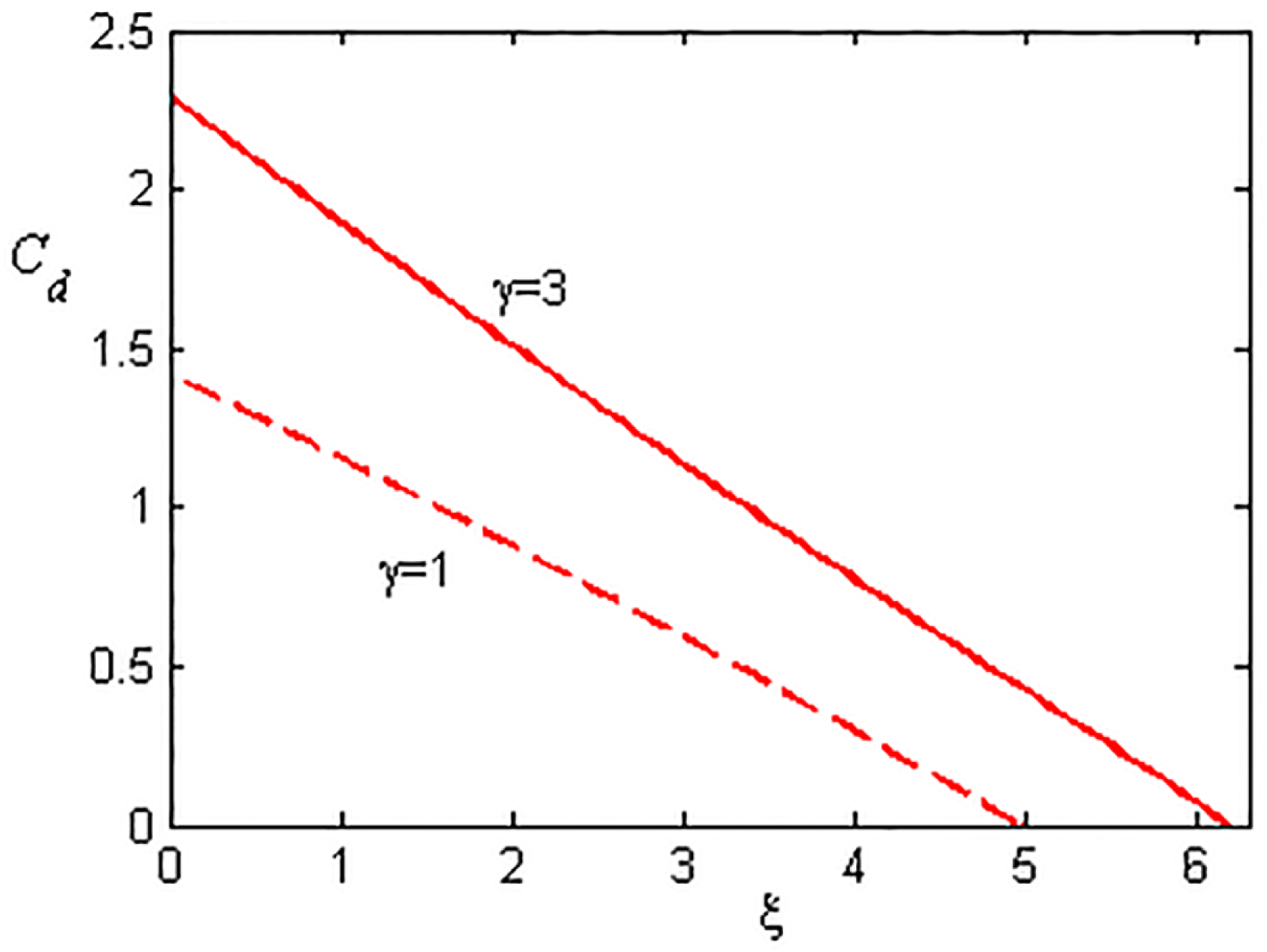
The variation
 $C_{d}$
with
 $\unicode[STIX]{x1D709}$
for
 $\unicode[STIX]{x1D6FF}=0.1$
,
 $Z=10$
,
 $\unicode[STIX]{x1D707}=0.8$
,
 $\unicode[STIX]{x1D6FE}=3$
(solid curve) representing the adiabatic expansion and
 $\unicode[STIX]{x1D6FE}=1$
(dashed cure) representing the isothermal expansion.

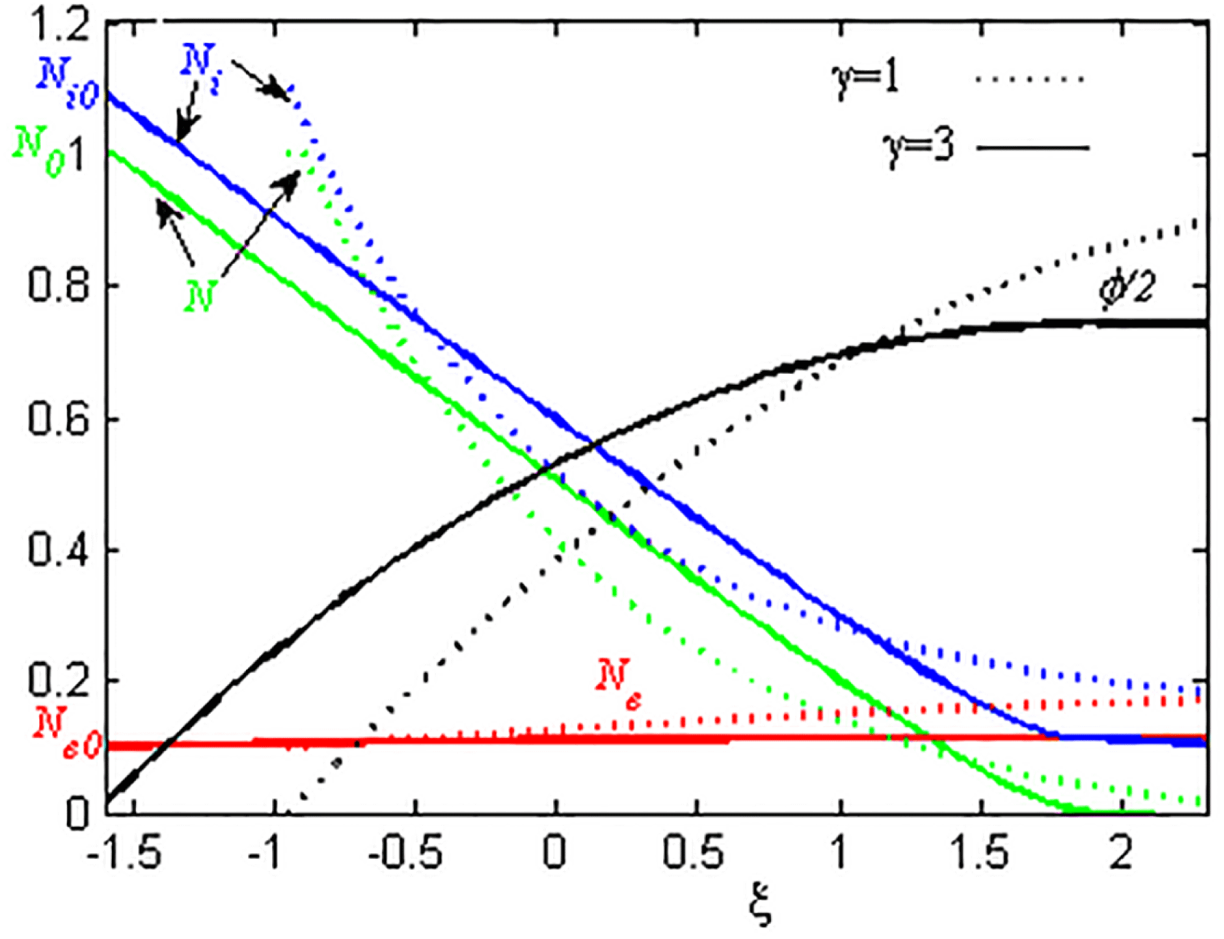
The variation
 $N$
,
 $N_{i}$
,
 $N_{e}$
and
 $\unicode[STIX]{x1D711}/2$
with
 $\unicode[STIX]{x1D709}$
for
 $\unicode[STIX]{x1D6FF}=0.1$
,
 $Z=10$
,
 $\unicode[STIX]{x1D707}=0.8$
,
 $\unicode[STIX]{x1D6FE}=3$
(solid curve) representing the adiabatic expansion and
 $\unicode[STIX]{x1D6FE}=1$
(dotted cure) representing the isothermal expansion.

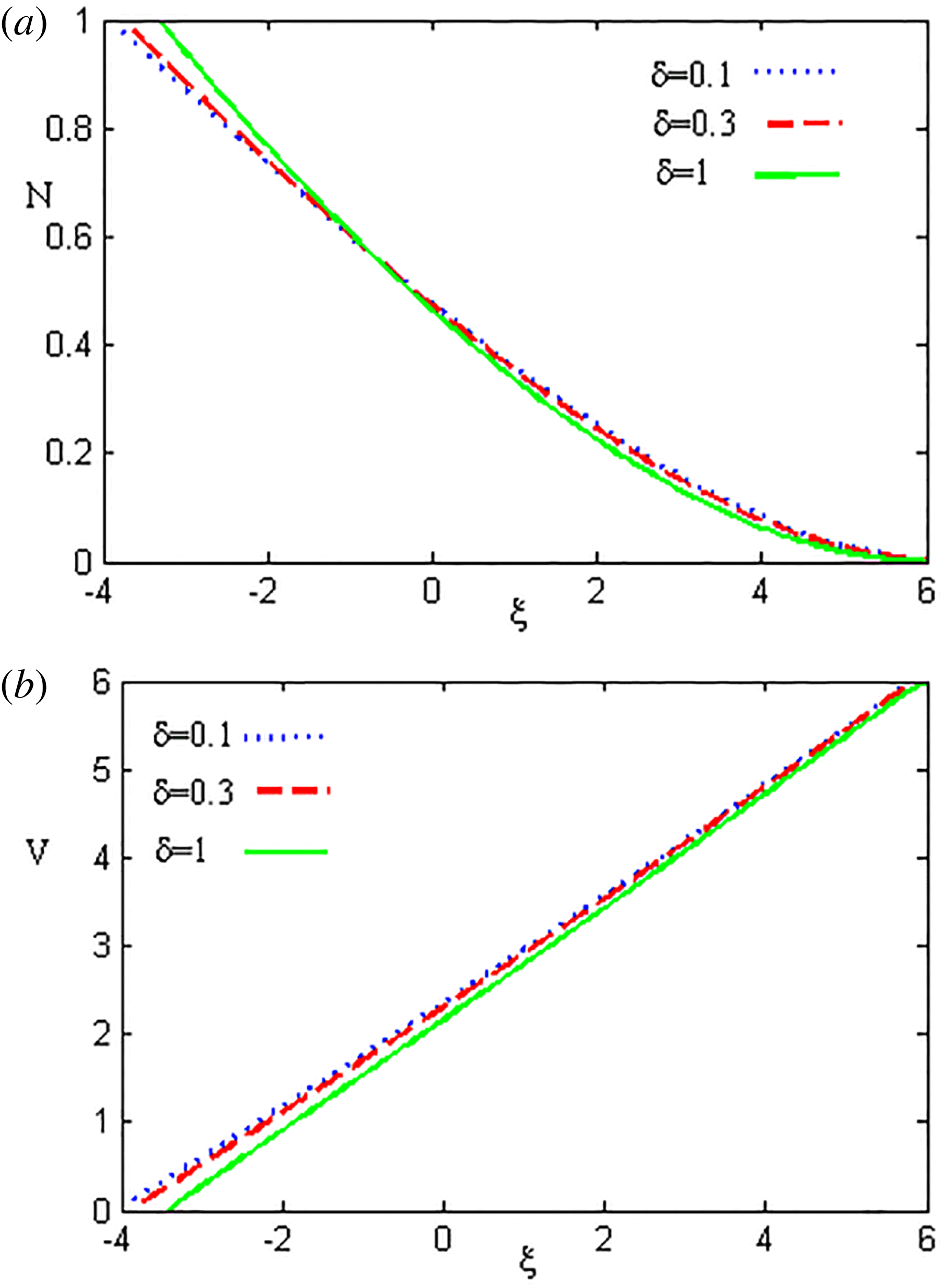
The variation (a)
 $N$
and (b)
 $V$
with
 $\unicode[STIX]{x1D709}$
for
 $\unicode[STIX]{x1D707}=0.8$
,
 $\unicode[STIX]{x1D6FE}=3$
,
 $\unicode[STIX]{x1D6FF}=0.1$
(dotted curve),
 $\unicode[STIX]{x1D6FF}=0.3$
(dashed curve),
 $\unicode[STIX]{x1D6FF}=1$
(solid curve).

We finally present some numerical solutions of the dusty plasma for the typical dusty plasma parameters:
 $\unicode[STIX]{x1D6FF}=0.1$
and
 $\unicode[STIX]{x1D707}=0.8$
. Our numerical analysis is based on the Runge–Kutta formula due to its high stability. The method accuracy has been tested by using the limiting conditions. The behaviour of a part of the velocity profile of the dusty plasma in terms of
 $C_{d}$
with respect to the self-similar variable
 $\unicode[STIX]{x1D709}$
is depicted in figure 1. It is observed that the effect of the adiabatic expansion (
 $\unicode[STIX]{x1D6FE}=3$
) causes an upwards shift in
 $C_{d}$
versus
 $\unicode[STIX]{x1D709}$
curve along the
 $C_{d}$
axis significantly, i.e. for fixed dusty plasma parameters
 $C_{d}$
has a larger (smaller) for adiabatic (isothermal) dusty plasma expansion. It is also clear that the adiabatic and isothermal dusty plasma expansions evolve with the different speeds, which are thus corresponding to the different expansion time scales. The behaviour of the dust, ion and electron number densities with the variation of the self-similar parameter
 $\unicode[STIX]{x1D709}$
is depicted for both adiabatic (
 $\unicode[STIX]{x1D6FE}=3$
) and isothermal (
 $\unicode[STIX]{x1D6FE}=1$
) situations in figure 2. It turns out that the adiabatic expansion is associated with cooling of the dust grains. This means that the adiabatic expansion ends earlier than the isothermal expansion does. The influence of the ratio (
 $\unicode[STIX]{x1D70E}$
) of ion temperature (
 $T_{i}$
) to electron temperature (
 $T_{e}$
) on the dust number density and the dust velocity have also been numerically examined. These are shown in figure 3, where the upper panel (figure 3
a) represents that for the higher values of
 $\unicode[STIX]{x1D6FF}$
in which the expansion takes place faster and the lower panel (figure 3
b) represents that the dust velocity increases with the increase of
 $\unicode[STIX]{x1D6FF}$
. This means that the warmer ions correspond to the higher dust velocity, and that an increase of
 $\unicode[STIX]{x1D6FF}$
leads to the acceleration of the dust particles and achievement to the higher energies. It should be added here that the increasing behaviour of the dust velocity cannot continue indefinitely since this corresponds to
 $N\rightarrow 0$
(figure 3
a) which has no physical meaning.
3.2 Warm dusty plasma limit,
$\unicode[STIX]{x1D6FC}\neq 0$

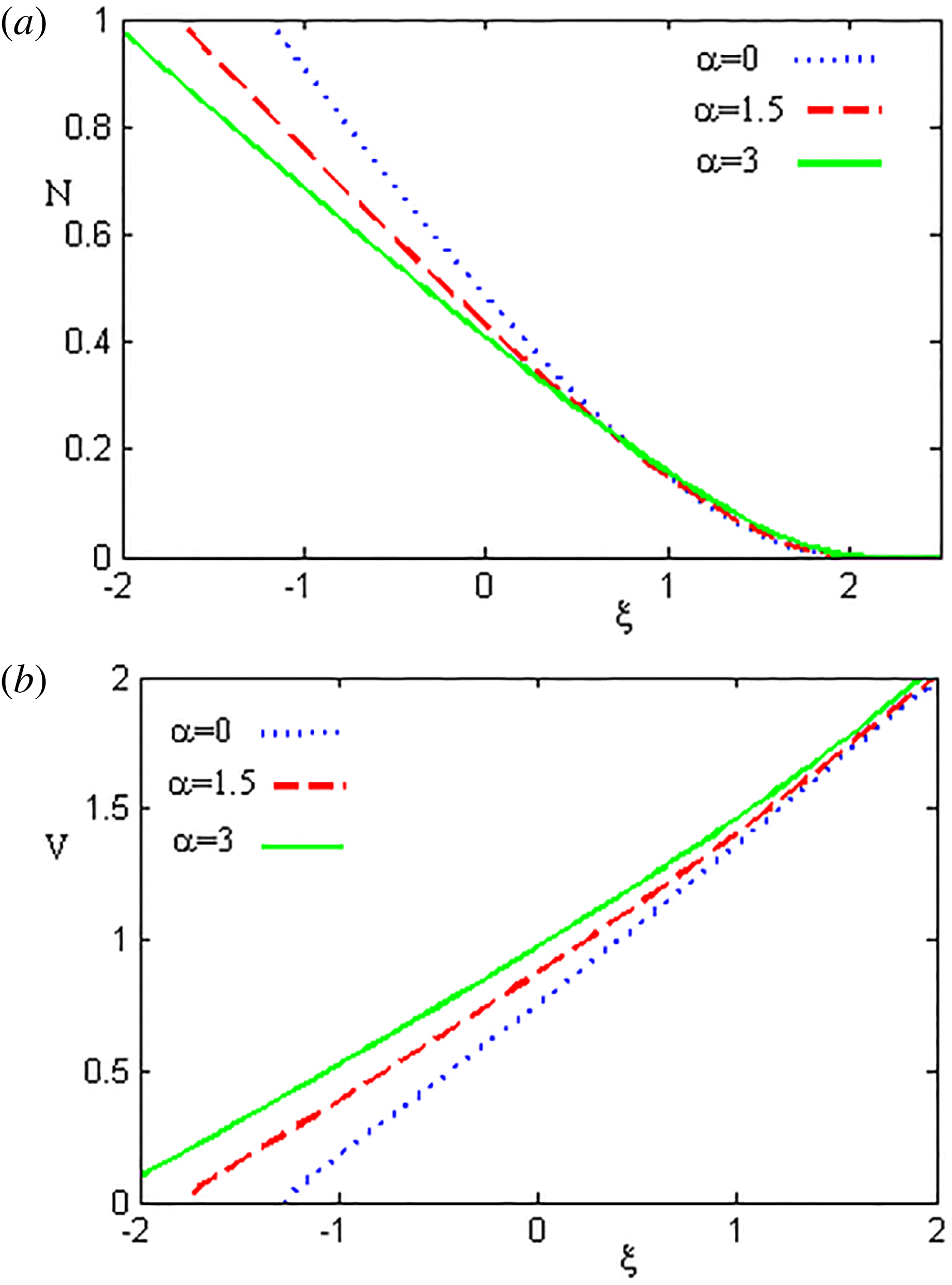
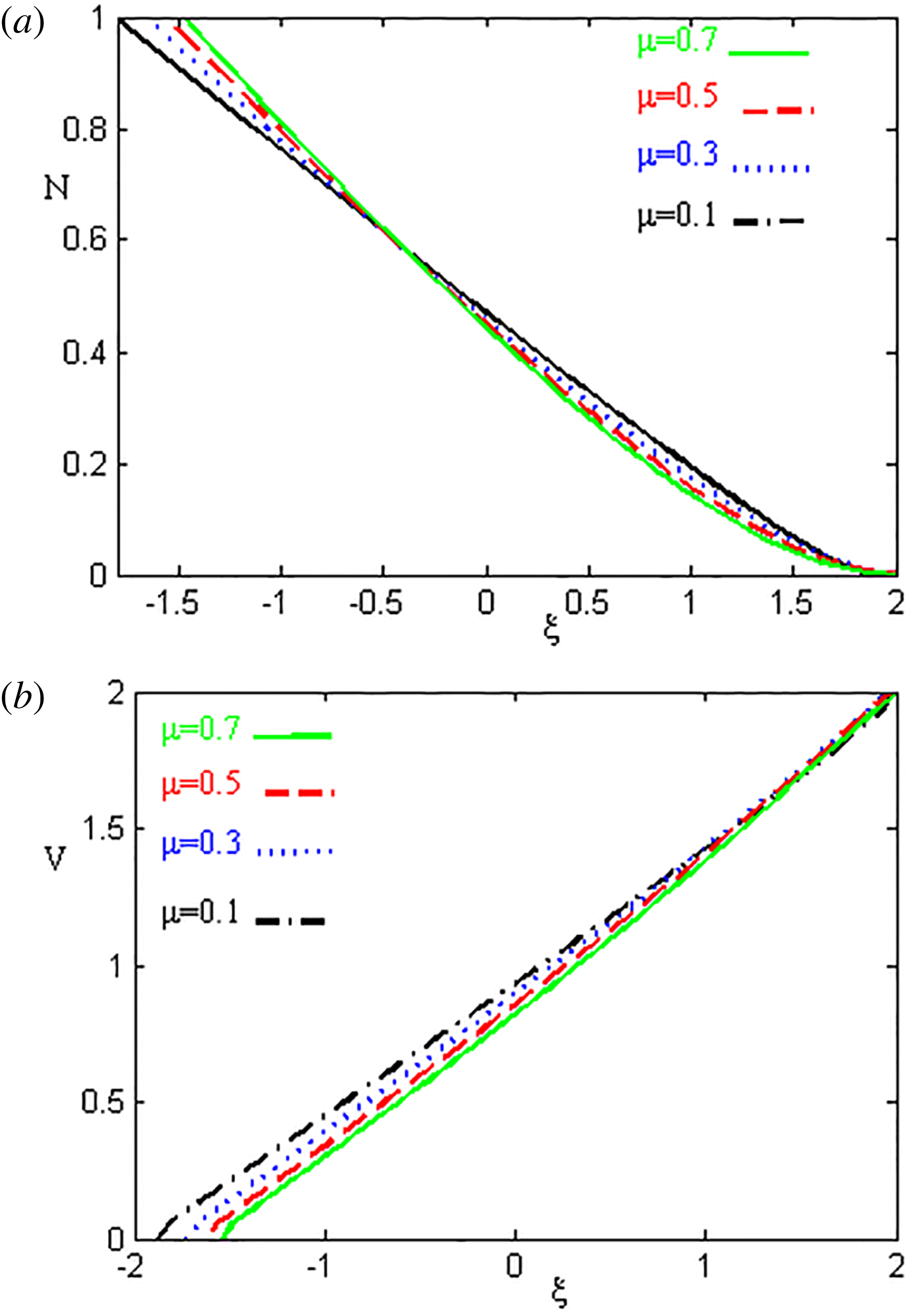
The variation of (a)
 $N$
and (b)
 $V$
with
 $\unicode[STIX]{x1D709}$
for
 $\unicode[STIX]{x1D6FF}=0.1$
,
 $\unicode[STIX]{x1D707}=0.8$
,
 $\unicode[STIX]{x1D6FE}=3$
,
 $\unicode[STIX]{x1D6FC}=0$
(solid curve),
 $\unicode[STIX]{x1D6FC}=1.5$
(dashed curve) and
 $\unicode[STIX]{x1D6FC}=3$
(dotted curve).

The variation if (a)
 $N$
and (b)
 $V$
with
 $\unicode[STIX]{x1D709}$
is for
 $\unicode[STIX]{x1D6FF}=0.1$
,
 $Z=10$
,
 $\unicode[STIX]{x1D6FE}=3$
and for
 $\unicode[STIX]{x1D707}=0.1$
, 0.3, 05, and 0.7.

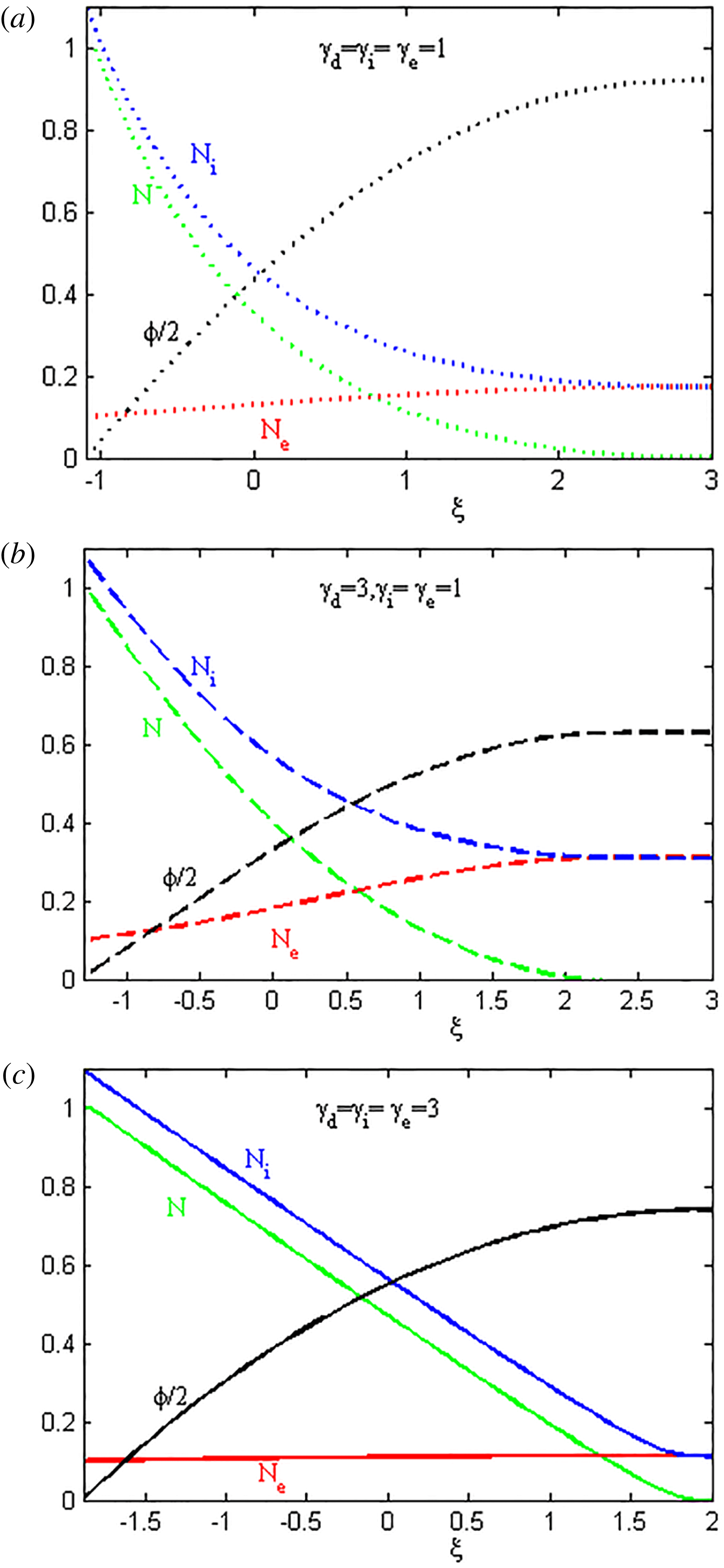
The variation of
 $N$
,
 $N_{i}$
,
 $N_{e}$
and
 $\unicode[STIX]{x1D711}/2$
with
 $\unicode[STIX]{x1D709}$
for
 $\unicode[STIX]{x1D6FF}=0.1$
,
 $Z=10$
,
 $\unicode[STIX]{x1D707}=0.8$
, (a)
 $\unicode[STIX]{x1D6FE}_{d}=\unicode[STIX]{x1D6FE}_{i}=\unicode[STIX]{x1D6FE}_{e}=1$
, (b)
 $\unicode[STIX]{x1D6FE}_{e}=\unicode[STIX]{x1D6FE}_{i}=1$
and
 $\unicode[STIX]{x1D6FE}_{d}=1$
and (c)
 $\unicode[STIX]{x1D6FE}_{d}=\unicode[STIX]{x1D6FE}_{i}=\unicode[STIX]{x1D6FE}_{e}=3$
.

We now examine the effect of the thermal pressure term by keeping it in the basic equations. We employ numerical analysis with suitable boundary conditions (providing for the plasma expansion requirements) to study the warm dusty plasma expansion. The initial conditions (which refer to an unperturbed dusty plasma) at an initial point
 $\unicode[STIX]{x1D709}_{0}$
are
 $\unicode[STIX]{x1D711}(\unicode[STIX]{x1D709}_{0})=v(\unicode[STIX]{x1D709}_{0})=0$
and
 $ZN(\unicode[STIX]{x1D709}_{0})=1$
, in which
 $\unicode[STIX]{x1D709}_{0}=-\sqrt{\unicode[STIX]{x1D6FE}/(1+\unicode[STIX]{x1D707}+\unicode[STIX]{x1D707}\unicode[STIX]{x1D6FF})+\unicode[STIX]{x1D6FC}}$
. We note that (3.6) is valid for
 $\unicode[STIX]{x1D6FC}=0.$
However, equation (3.6) can be generalized to
 $\unicode[STIX]{x1D6FC}\neq 0$
, and can be expressed as
 $$\begin{eqnarray}\frac{\text{d}\unicode[STIX]{x1D711}}{\text{d}\unicode[STIX]{x1D709}}=K(\unicode[STIX]{x1D711}),\end{eqnarray}$$
where
 $$\begin{eqnarray}K(\unicode[STIX]{x1D711})=\frac{2\sqrt{G(\unicode[STIX]{x1D711})F(\unicode[STIX]{x1D711})^{3}+\unicode[STIX]{x1D6FC}(G(\unicode[STIX]{x1D711}))^{\unicode[STIX]{x1D6FE}-1}}}{[3F(\unicode[STIX]{x1D711})^{2}+G(\unicode[STIX]{x1D711})F^{\prime }(\unicode[STIX]{x1D711})+\unicode[STIX]{x1D6FC}(\unicode[STIX]{x1D6FE}+1)F(\unicode[STIX]{x1D711})^{3}(G(\unicode[STIX]{x1D711}))^{\unicode[STIX]{x1D6FE}-2}]}.\end{eqnarray}$$
Now, we numerically examine the effects of dust temperature (
 $\unicode[STIX]{x1D6FC}$
) on the adiabatic expansion of the dusty plasma, and have graphically shown how dust number density
 $N$
and dust speed
 $V$
variations for different values of
 $\unicode[STIX]{x1D6FC}$
in figure 4, which shows that by increasing of
 $\unicode[STIX]{x1D6FC}$
, the dust number density
 $N$
decreases (figure 4
a), but the dust particle speed
 $V$
increases (figure 4
b). This means that the adiabatic expansion of the dusty plasma increases as we increase the dust temperature. We have also graphically shown how the dust number density
 $N$
and dust speed
 $V$
vary for different values of the initial electron population (represented by
 $\unicode[STIX]{x1D707}$
). These are depicted in figure 5, which shows that, as we increase
 $\unicode[STIX]{x1D707}$
, the value of
 $N$
decreases (increases) for
 $\unicode[STIX]{x1D709}<-0.5$
(
 $\unicode[STIX]{x1D709}>0.5$
) (figure 5
a), and the dust speed
 $V$
decreases for the whole range of
 $\unicode[STIX]{x1D709}$
(figure 5
b). We finally graphically compare the isothermal and isentropic expansion of the dusty plasma under consideration. These are displayed in figure 6, where the uppermost panel (figure 6
a) is for
 $\unicode[STIX]{x1D6FE}_{e}=\unicode[STIX]{x1D6FE}_{i}=\unicode[STIX]{x1D6FE}_{d}=1$
; the middle panel (figure 6
b) is for
 $\unicode[STIX]{x1D6FE}_{e}=\unicode[STIX]{x1D6FE}_{i}=1$
and
 $\unicode[STIX]{x1D6FE}_{d}=3$
and the lower panel (figure 6
c) is for
 $\unicode[STIX]{x1D6FE}_{e}=\unicode[STIX]{x1D6FE}_{i}=\unicode[STIX]{x1D6FE}_{d}=3$
. These figures indicate that (i) the increase in the dusty plasma expansion increases as more plasma components deviate from isothermal to adiabatic behaviour; (ii) with the deviation from isothermal behaviour, the plasma expansion becomes faster, and it reaches its maximum rate; and (iii) the adiabatic expansion leads to the cooling of the dust particles, thus the adiabatic expansion ends earlier than that of the isothermal one.
4 Discussion
We have investigated the influence of adiabaticity of the dusty plasma species (viz. dust, electrons and ions) on the expansion mechanism of the dust, ion and electron species in an unmagnetized dusty plasma. The results, which have been found from this theoretical investigation, can be pinpointed as follows:
-
(i) The dusty plasma expansion depends only on the self-similar quantity
$\unicode[STIX]{x1D709}$
. It is seen that when the dust number density tends to zero, the ion and electron number densities become equal. It turns out that the dust particles are accelerated to some maximum velocity. Therefore, after a finite value of the self-similar quantity
$\unicode[STIX]{x1D709}$
, the dusty plasma becomes free from the dust particles during its expansion. -
(ii) The adiabaticity of dusty plasma species significantly modifies the dusty plasma expansion procedure. It is found that the dusty plasma expansion in the presence of the adiabaticity effect takes place faster than that of the isothermal case since the adiabatic expansion leads to cooling of the dust particles. To make a comparison, we have considered three different cases (i)
$\unicode[STIX]{x1D6FE}_{d}=\unicode[STIX]{x1D6FE}_{i}=\unicode[STIX]{x1D6FE}_{e}=1$
, (ii)
$\unicode[STIX]{x1D6FE}_{d}=3$
,
$\unicode[STIX]{x1D6FE}_{i}=\unicode[STIX]{x1D6FE}_{e}=1$
, (corresponding to that considered by Bharuthram & Rao Reference Bharuthram and Rao1995) and (iii)
$\unicode[STIX]{x1D6FE}_{d}=\unicode[STIX]{x1D6FE}_{i}=\unicode[STIX]{x1D6FE}_{e}=3$
. The numerical analysis indicates that the expansion rate increases from case (i) to (iii), as the third case refers to faster expansion. Our result in the case of
$\unicode[STIX]{x1D6FE}_{d}=3$
,
$\unicode[STIX]{x1D6FE}_{i}=\unicode[STIX]{x1D6FE}_{e}=1$
, are in good agreement with those reported by Bharuthram & Rao (Reference Bharuthram and Rao1995). It is also found that the effect of adiabaticity of dusty plasma species depends on the relevant physical parameters
$\unicode[STIX]{x1D707}$
,
$\unicode[STIX]{x1D6FF}$
and
$\unicode[STIX]{x1D6FC}$
. -
(iii) The adiabatic and isothermal dusty plasma expansions evolve with the different acoustic speeds, which thus correspond to different expansion time scales.
-
(iv) The expansion rate is very sensitive to different relevant dusty plasma parameters, such as the initial electron population
$\unicode[STIX]{x1D707}$
, the ratio of ion temperature to electron temperature
$\unicode[STIX]{x1D6FF}$
and the dust temperature parameter
$\unicode[STIX]{x1D6FC}$
. It is found that the higher values of the initial population of electrons corresponds to higher values of the dust velocity. As a result, for the higher values of
$\unicode[STIX]{x1D707}$
, the expansion takes place faster, and the dust particles are accelerated to higher energies rather than those at the lower values of
$\unicode[STIX]{x1D707}$
.


We note that the effects of the strong external magnetic field (Shahmansouri & Mamun Reference Shahmansouri and Mamun2014b
) (which is needed to magnetize the massive dust particles), the dust charge fluctuation (which is important for the expansion associated with the waves, whose frequency is compared to the dust charging frequency) and the strong interaction between dust grains (Shahmansouri & Rezaei Reference Shahmansouri and Rezaei2014; Shahmansouri & Alinejad Reference Shahmansouri and Alinejad2015) on the dusty plasma expansion can be problems of great importance, and beyond the scope of our present investigation. However, the effect of the dust charge fluctuation on the dusty plasma expansion is not important since the latter is associated with the dust-acoustic waves, whose frequency is not comparable to the dust charging frequency. On the other hand, the magnetic field is not strong enough to magnetize the massive dust particles which occur in most space and laboratory dusty plasma situations. It should be added here that the means for cooling of the dusty plasma system under consideration is the decrease of thermodynamic pressure. However, for study of the temperature (
 $T$
) evolution,
 $T$
is required as another dynamical quantity (i.e.
 $T=T(\unicode[STIX]{x1D719})$
). This is a similar situation to that considered by McQuillen et al. (Reference McQuillen, Strickler, Langin and Killian2015). Thus, to include the effect of
 $T=T(\unicode[STIX]{x1D719})$
on our present work can be an interesting research problem for our future study. It may also be noted that we have tried our best to consider a wide range of physical systems in which all of the plasma species can be adiabatic. We made a systematic investigation regarding the adiabaticity parameters, and thus our results may be applicable to a number of astrophysical and space dusty plasmas as well as to future dusty plasma laboratory experiments.