1 Introduction
The modelling and forecasting of mortality play a fundamental part in the working life of an actuary. It is widely known that human mortality depends on an individual’s current age, the current year and their year of birth (among many other possible risk factors). These determinants of mortality are generally known as the age effect, the period effect and the cohort effect, respectively. There is a tried and tested method of approaching the problem. We define a model for the force of mortality which depends on the age, the period and usually (but not always) the cohort effect. The parameters are estimated from some suitable data. The period and cohort parameters are then forecast, and from these estimated and forecast values, the forecast values of mortality are obtained. Examples of such models are the Lee–Carter model (Lee & Carter, Reference Lee and Carter1992), the age-period-cohort model (Clayton & Schifflers, Reference Clayton and Schifflers1987b) and various forms of the Cairns–Blake–Dowd (CBD) model (Cairns et al., Reference Cairns, Blake, Dowd, Coughlan, Epstein, Ong and Balevich2009). More recently, the Continuous Mortality Investigation or CMI introduced the age-period-cohort-improvements model (Continuous Mortality Investigation, 2016a, 2016b, 2016c). For a particular model, the method can be summarised in the following three steps: (1) estimate the age, period and cohort parameters, (2) forecast the period and cohort parameters and (3) obtain the forecast values of mortality.
There is a difficulty. The models mentioned above do not allow the unique estimation of the parameter sets without the introduction of some further assumptions. The standard approach is to place some constraints on the estimates, such as the period effects are constrained to sum to zero. There is no reason why two actuaries working independently should use the same constraints; they will obtain different estimates of the age, period and cohort effects. Indeed, Clayton & Schifflers (Reference Clayton and Schifflers1987b) in a carefully argued paper warn against the forecasting of cohort effects in particular. This is often referred to as the “identifiability problem”; see Cairns et al. (Reference Cairns, Blake, Dowd, Coughlan, Epstein, Ong and Balevich2009), Continuous Mortality Investigation (2016a, 7.3) and Richards et al. (to appear).
In our paper, we take the view that the estimates of the age, period and cohort effects are of interest to the actuary only as intermediate quantities; they are used to obtain the quantities of interest, namely, the forecast values of mortality. Apart from the Lee–Carter model, the models mentioned above are all examples of generalised linear models or GLMs (Nelder & Wedderburn, Reference Nelder and Wedderburn1972). It is a basic result that, while the parameters in the GLMs mentioned above are not identifiable, the fitted values (of mortality) are identifiable (Continuous Mortality Investigation, 2016a, 7.3), i.e., invariant with respect to the choice of constraints on the parameters. The main result in our paper is that the forecast values of mortality are also identifiable when the period and cohort effects are forecast with an autoregressive integrated moving average or ARIMA model with fitted mean: two actuaries working independently may not obtain the same estimates of the age, period and cohort effects, but they will obtain the same forecasts of mortality.
The problem of identifiability in the forecasting of mortality has received considerable attention within both the actuarial and the statistical literature. Hunt & Blake (Reference Hunt and Blake2020a, Reference Hunt and Blake2020b, Reference Hunt and Blake2020c) in a series of papers discuss the problem for a general class of age-period models (of which the Lee–Carter model is a simple example) and for this class with an added cohort effect. They emphasise the arbitrary nature of a particular set of identifiability constraints and the importance of using a forecasting method which does not depend on this arbitrary choice. They call such a method “well-identified”, discuss how to choose such a forecasting method and provide some examples.
The plan of the paper is as follows: in section 2, we describe the data we use to illustrate our results, set out our notation and define the class of model we discuss. In section 3, we state the fundamental result on invariance of fitted values in a GLM in terms of the null space of the model matrix; this section also contains the necessary theory for estimation in a GLM in which some parameters are subject to constraints and/or smoothing. Section 4 contains our four examples: the age-period, age-period-cohort, age-period-cohort-improvements and Lee–Carter models. We make some concluding remarks in section 5. There are three appendices. Appendix A gives the matrix theory underlying the use of null spaces as applied to GLMs. Appendix B shows how invariance can be exploited to give a simple way of fitting GLMs with specified constraints. In Appendix C, we give a proof of the time series result used to show the invariance of forecasting with respect to the choice of constraints.
2 Data, Notation and the Basic Model
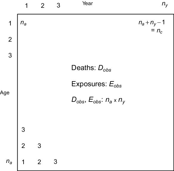
We illustrate our ideas with data from the Office for National Statistics on UK males. The data comprise the deaths and central exposures for ages 50–104 and years 1971–2015. These data lie naturally in a matrix with rows indexed by age and columns indexed by year. We adopt the convention that matrices are denoted by upper case bold font as in  $\textbf{\textit{X}}$
and column vectors by lower case bold font as in
 $\textbf{\textit{x}}$
. With this in place, we denote the age indices by
 $\textbf{\textit{x}}_a= (1,\ldots, n_a)^\prime$
and the year indices by
 $\textbf{\textit{x}}_y =(1,\ldots, n_y)^\prime$
, where the
 $^\prime$
indicates the transpose of a vector (or matrix); this simplifies the notation without jeopardising the presentation. The data thus comprise two matrices:
 $\textbf{\textit{D}}_{obs} = (d_{x, y})$
, the matrix of the number of deaths at age x in year y, and
 $\textbf{\textit{E}}_{obs} = (e_{x, y})$
, the total time lived or central exposure at age x in year y. (We will use
 $\textbf{\textit{D}}$
later to denote a difference matrix.) Thus,
 $\textbf{\textit{D}}_{obs}$
and
 $\textbf{\textit{E}}_{obs}$
are both
 $n_a \times n_y$
. Furthermore, we label the cohorts with
 $\boldsymbol{x}_c = (1,\ldots, n_c)^\prime$
, where
 $n_c = n_a + n_y -1$
is the number of distinct cohorts. We adopt the convention that the oldest cohort, i.e., for age
 $n_a$
in year 1, is indexed 1; hence, the cohort index for cell (i, j) is
 $c(i, j) = n_a - i + j$
. In our example, we have
 $n_a = 55$
,
 $n_y = 45$
and
 $n_c = 99$
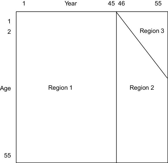
. Figure 1 summarises our notation.
Age of death = rows, year of death = columns, year of birth = diagonals downwards from left to right.

In addition, the following notation is useful:  $\textbf{1}_n$
denotes a column vector of 1s of length n and
 $\textbf{\textit{I}}_n$
denotes the identity matrix of size n. Furthermore, we let
 $\textbf{0}_n$
stand for either a column vector of 0s of length n or an
 $n \times n$
zero matrix; the context should make clear which applies. We may omit the suffix n if no confusion results. We will make frequent use of the Kronecker product, which we denote
 $\otimes$
; see Macdonald et al. (Reference Macdonald, Richards and Currie2018, chapter 12) for examples of the Kronecker product as used in expressing models of mortality.
We assume that  $D_{x, y}$
, the random variable corresponding to the observed deaths
 $d_{x, y}$
, follows the Poisson distribution with mean
 $e_{x, y} \mu_{x, y}$
, where
 $\mu_{x, y}$
is the force of mortality at age x in year y, i.e.,
 $D_{x, y} \sim \mathcal{P}(e_{x, y} \mu_{x, y})$
. We note that there is a slight abuse of notation here; strictly, we should write
 $\mu_{x+1/2, y+1/2}$
since
 $e_{x, y}$
is the central exposure; we will use the simpler notation throughout for clarity. Let
 $\mbox{vec}(\textbf{\textit{M}})$
be the function that stacks the columns of a matrix
 $\textbf{\textit{M}}$
on top of each other in column order. Let
 $\textbf{\textit{d}} =\mbox{vec}(\textbf{\textit{D}}_{obs})$
and
 $\textbf{\textit{e}} = \mbox{vec}(\textbf{\textit{E}}_{obs})$
be the stacked vectors of deaths and exposures; let
 $\boldsymbol{\mu}$
be the corresponding vector of forces of mortality. We consider models where
 $\log \boldsymbol{\mu}$
can be written in the following form:
 \begin{equation}\log \boldsymbol{\mu} = \textbf{\textit{X}} \boldsymbol{\theta}\end{equation}
Together with the Poisson assumption, this defines a generalised linear model or GLM with model matrix  $\textbf{\textit{X}}$
, log link and Poisson error; the exposure enters into the model definition as an offset,
 $\log\textbf{\textit{e}}$
. This is a very wide class of model and includes the Gompertz model (in one dimension), the age-period or AP model, the age-period-cohort or APC model, various forms of the CBD models, and the CMI’s age-period-cohort-improvements or APCI model. The Lee–Carter model, although not immediately in this class, can also be included, as we will show in section 4.4.
3 Models and Null Spaces
We assume that we have a GLM with model matrix  $\textbf{\textit{X}}$
, regression coefficients
 $\boldsymbol{\theta}$
, a log link and a Poisson error distribution. We suppose that
 $\textbf{\textit{X}}$
is
 $n \times p, \,n > p$
, with rank
 $p - q$
where
 $q \ge 1$
; see Appendix A for a brief discussion of rank. We denote the rank of
 $\textbf{\textit{X}}$
by
 $r(\textbf{\textit{X}})$
. The model matrix is not of full rank; this implies that the estimates of
 $\boldsymbol{\theta}$
are not unique. However, if we specify a set of q linearly independent constraints
 $\textbf{\textit{H}} \boldsymbol{\theta} = \textbf{0}_q$
, where
 \begin{equation*} \left(\begin{array}{c} \textbf{\textit{X}} \\[3pt] \textbf{\textit{H}}\end{array}\right)\end{equation*}
has full rank p, then we do have a unique estimate of  $\boldsymbol{\theta}$
. In general, the idea is to choose
 $\textbf{\textit{H}}$
so that the components of the resulting estimate have a natural interpretation and can be forecast. All the models considered in this paper have model matrices which are not of full rank.
Suppose  $\hat {\boldsymbol{\theta}}_1$
and
 $\hat {\boldsymbol{\theta}}_2$
are two estimates of
 $\boldsymbol{\theta}$
subject to the constraints
 $\textbf{\textit{H}}_1 \boldsymbol{\theta} = \textbf{\textit{H}}_2 \boldsymbol{\theta} = \textbf{0}_q$
, respectively. We wish to understand the relationship between
 $\hat {\boldsymbol{\theta}}_1$
and
 $\hat{\boldsymbol{\theta}}_2$
. This relationship is characterised by the null space of
 $\textbf{\textit{X}}$
,
 $\mathcal{N}(\textbf{\textit{X}}) = \{\textbf{\textit{v}}:\ \textbf{\textit{X}} \textbf{\textit{v}} = \textbf{0}\}$
. To be precise
 \begin{equation}\hat {\boldsymbol{\theta}}_1 - \hat {\boldsymbol{\theta}}_2 \in \mathcal{N}(\textbf{\textit{X}})\end{equation}
see Appendix A for a proof of this fundamental result. Thus,  $\mathcal{N}(\textbf{\textit{X}})$
will tell us how the estimates of
 $\boldsymbol{\theta}$
under different constraint systems are related; ideally, a forecast will not depend on this choice. We note in particular that
 $\hat {\boldsymbol{\theta}}_1 - \hat {\boldsymbol{\theta}}_2 \in \mathcal{N}(\textbf{\textit{X}})$
implies that
 \begin{equation} \textbf{\textit{X}} \hat {\boldsymbol{\theta}}_1 = \textbf{\textit{X}} \hat {\boldsymbol{\theta}}_2\end{equation}
in other words, the fitted values of log mortality are equal, an example of the general result that the fitted values in a GLM are equal under different constraint systems.
It is often advantageous to smooth certain terms in a model of mortality. We will use the P-spline system of smoothing; see Eilers & Marx (Reference Eilers and Marx1996), Macdonald et al. (Reference Macdonald, Richards and Currie2018, chapter 11). The idea is to replace a parameter,  $\boldsymbol{\alpha}$
say, by a smooth function,
 $\textbf{\textit{B}}\textbf{\textit{a}}$
, where
 $\textbf{\textit{B}}$
is a regression matrix evaluated over a basis of B-splines; we use cubic B-splines throughout. In our examples,
 $\boldsymbol{\alpha}$
will be an age parameter, and for technical reasons, we will always place a knot at the first age. The regression coefficients
 $\textbf{\textit{a}}$
are then subject to a penalty which penalises local differences in
 $\textbf{\textit{a}}$
.
Let  $\boldsymbol{\alpha} = \textbf{\textit{B}} \textbf{\textit{a}}$
, where
 $\textbf{\textit{B}}$
is
 $n_a \times c_a$
and
 $\textbf{\textit{a}} = (a_1, \ldots, a_{c_a})^\prime$
. The second-order penalty on
 $\textbf{\textit{a}}$
is
 \begin{equation}(a_1 - 2a_2 + a_3)^2 + \ldots + (a_{c_a-2} - 2 a_{c_a-1} + a_{c_a})^2\end{equation}
We write this compactly by defining  $\textbf{\textit{D}}$
, the difference matrix of order two, as
 \begin{equation} \textbf{\textit{D}} = \left[\begin{array}{ccccccc} 1 & \quad -2 & \quad 1 & \quad 0 & \quad 0 & \quad 0 & \quad \cdots \\[6pt]
0 & \quad 1 & \quad -2 & \quad 1 & \quad 0 & \quad 0 &\quad \cdots \\[6pt]
0 & \quad 0 & \quad 1 & \quad -2 & \quad 1 & \quad 0 & \quad \cdots \\[6pt]
\vdots & \quad \vdots & \quad \vdots & \quad \vdots & \quad \vdots & \quad \vdots & \quad \ddots\end{array}\right],\; (c_a-2) \times c_a\end{equation}
With this notation, the quadratic penalty (4) can be written as
 \begin{equation} \textbf{\textit{a}}^\prime \textbf{\textit{D}}^\prime \textbf{\textit{D}} \textbf{\textit{a}}\end{equation}
We make the important remark that  $r(\textbf{\textit{D}})$
is
 $c_a-2$
and so the dimension of the null space of
 $\textbf{\textit{D}}$
,
 $\mathcal{N}(\textbf{\textit{D}})$
, is two. A basis for
 $\mathcal{N}(\textbf{\textit{D}})$
is
 $\{\textbf{\textit{n}}_1, \textbf{\textit{n}}_2\}$
, where
 $\textbf{\textit{n}}_1 =\textbf{1}_{c_a}$
and
 $\textbf{\textit{n}}_2 = (1,2,\ldots, c_a)^\prime$
. We will be interested in the relationship between
 $\mathcal{N}(\textbf{\textit{D}})$
and
 $\mathcal{N}(\textbf{\textit{X}})$
since this can affect the number of constraints required to enable parameters to be estimated uniquely. Proposition 4 in Appendix A describes this relationship, which is illustrated in our discussion of our examples in section 4.
The strength of the penalty is determined by the smoothing parameter  $\lambda,$
and, from (6), we define the penalty matrix
 \begin{equation} \textbf{\textit{P}} = \lambda \textbf{\textit{D}}^\prime \textbf{\textit{D}}\end{equation}
Clearly, if  $\lambda$
is small the coefficients will be less smooth, while if
 $\lambda$
is large the coefficients will be more smooth.
We have described a penalty of order two but penalties of other orders can be used. For example, in his landmark paper on graduation, Whittaker (Reference Whittaker1923) used a third-order penalty with terms like  $(a_1 -3a_2 +3 a_3 - a_4)^2$
. If
 $\textbf{\textit{D}}$
is the resulting difference matrix, then
 $\mathcal{N}(\textbf{\textit{D}}) = \{\textbf{\textit{n}}_1, \textbf{\textit{n}}_2, \textbf{\textit{n}}_3\},$
where
 $\textbf{\textit{n}}_1$
and
 $\textbf{\textit{n}}_2$
are as in the previous paragraph and
 $\textbf{\textit{n}}_3 =(1^2,2^2,\ldots, c_a^2)^\prime$
. The first-order penalty has terms like
 $(a_1 - a_2)^2$
, and the null space of the corresponding difference matrix consists of
 $\textbf{\textit{n}}_1$
only. In general, we denote the order of the penalty by d. A basis for the null space of a difference matrix of order d is given by
 $\{\textbf{\textit{n}}_1, \ldots, \textbf{\textit{n}}_d\}$
, where
 \begin{equation} \textbf{\textit{n}}_j = (1^{j-1}, 2^{j-1}, \ldots, c_a^{j-1})^\prime,\, j = 1, \ldots, d\end{equation}
We describe a general approach to fitting GLMs that are subject to both constraints and smoothing. Nelder and Wedderburn (Reference Nelder and Wedderburn1972) introduced GLMs and showed that estimation in a GLM is given by
 \begin{equation} \textbf{\textit{X}}^\prime \tilde {\textbf{\textit{W}}} \textbf{\textit{X}} \hat {\boldsymbol{\theta}} = \textbf{\textit{X}}^\prime \tilde {\textbf{\textit{W}}} \tilde {\textbf{\textit{z}}}\end{equation}
where the tilde, as in  $\tilde {\boldsymbol{\theta}}$
, indicates a current estimate, while
 $\hat {\boldsymbol{\theta}}$
indicates an improved approximation in the iterative scheme. The matrix
 $\tilde {\textbf{\textit{W}}}$
is the diagonal matrix of weights and the vector
 $\tilde {\textbf{\textit{z}}}$
is the so-called working variable. For Poisson errors and a log link,
 $\tilde {\textbf{\textit{W}}}$
and
 $\tilde {\textbf{\textit{z}}}$
are
 \begin{equation} \tilde {\textbf{\textit{W}}} = \mbox{diag}\{\,\tilde {\!\textbf{\textit{d}}} \},\; \tilde {\textbf{\textit{z}}} = \textbf{\textit{X}} \tilde {\boldsymbol{\theta}} + \left({\textbf{\textit{d}} \over \tilde {\!\textbf{\textit{d}}}} - \textbf{1}\right)\end{equation}
where  $\,\tilde {\!\textbf{\textit{d}}}$
indicates the current estimate of the fitted deaths and
 $\textbf{\textit{d}}/\, \tilde {\!\textbf{\textit{d}}}$
indicates element-by-element division.
A possible and easily overlooked complication may arise when  $\boldsymbol{\theta}$
(or some portion of
 $\boldsymbol{\theta})$
is smoothed. With P-splines, equation (9) becomes
 \begin{equation} (\textbf{\textit{X}}^\prime \tilde {\textbf{\textit{W}}} \textbf{\textit{X}} + \textbf{\textit{P}}) \hat {\boldsymbol{\theta}} = \textbf{\textit{X}}^\prime \tilde {\textbf{\textit{W}}} \tilde {\textbf{\textit{z}}}\end{equation}
where  $\textbf{\textit{P}}$
is the penalty matrix (Currie et al., Reference Currie, Durban and Eilers2004). The number of constraints required for (11) to have a unique solution is now determined by
 $r(\textbf{\textit{X}}^\prime \tilde {\textbf{\textit{W}}} \textbf{\textit{X}} +\textbf{\textit{P}})$
and not by
 $r(\textbf{\textit{X}}^\prime \tilde {\textbf{\textit{W}}} \textbf{\textit{X}}) = r(\textbf{\textit{X}})$
. Fortunately, for most models of mortality, we do have
 $r(\textbf{\textit{X}}^\prime\tilde {\textbf{\textit{W}}} \textbf{\textit{X}} + \textbf{\textit{P}}) = r(\textbf{\textit{X}})$
, but there are cases when
 $r(\textbf{\textit{X}})$
is strictly less than
 $r(\textbf{\textit{X}}^\prime \tilde {\textbf{\textit{W}}} \textbf{\textit{X}}+ \textbf{\textit{P}})$
, so it is best to be aware of this possible pitfall. In such cases, the number of constraints required to yield a unique estimate of
 $\boldsymbol{\theta}$
will be reduced; some examples are given in section 4, notably for the APCI model. This discussion suggests the following definition.
Definition:The effective rank of a model with model matrix  $\textbf{\textit{X}}$
and penalty
 $\textbf{\textit{P}}$
is
 \begin{equation} r(\textbf{\textit{X}}^\prime \tilde {\textbf{\textit{W}}} \textbf{\textit{X}} + \textbf{\textit{P}})\end{equation}
We show in Proposition A.4 in Appendix A that
 \begin{equation} \mathcal{N}(\textbf{\textit{X}}^\prime \tilde {\textbf{\textit{W}}} \textbf{\textit{X}} + \textbf{\textit{P}}) = \mathcal{N}(\textbf{\textit{X}}^\prime \tilde {\textbf{\textit{W}}} \textbf{\textit{X}}) \cap \mathcal{N}(\textbf{\textit{P}}) = \mathcal{N}(\textbf{\textit{X}}) \cap \mathcal{N}(\textbf{\textit{P}})\end{equation}
and so
 \begin{equation} r(\textbf{\textit{X}}^\prime \tilde {\textbf{\textit{W}}} \textbf{\textit{X}} + \textbf{\textit{P}}) \ge r(\textbf{\textit{X}})\end{equation}
Thus, smoothing can never increase the number of constraints required to obtain unique estimates of  $\boldsymbol{\theta}$
. The effective rank of a model has connections with the widely used effective dimension of a model but is a distinct idea; see Macdonald et al. (2018, chapter 11) for a discussion of effective dimension.
In our case,  $\textbf{\textit{X}}$
is not of full rank; equation (9) is singular and cannot be solved. The R package (R Core Team, 2018) has its own way of dealing with this problem, but we want solutions that satisfy particular constraints and where some components of
 $\boldsymbol{\theta}$
may be subject to smoothing. Currie (Reference Currie2013) generalised equation (9) to deal with this case and showed that
 \begin{align} \left(\begin{array}{ccc} \textbf{\textit{X}}^\prime \tilde {\textbf{\textit{W}}} \textbf{\textit{X}} + \textbf{\textit{P}} & \quad :& \quad \textbf{\textit{H}}^\prime \\[5pt]
\textbf{\textit{H}} & \quad :& \quad \textbf{0} \end{array} \right) \left(\begin{array}{c} \hat {\boldsymbol{\theta}} \\[5pt] \hat {\boldsymbol{\omega}} \end{array} \right) = \left(\begin{array}{c} \textbf{\textit{X}}^\prime \tilde {\textbf{\textit{W}}} \tilde {\textbf{\textit{z}}} \\[5pt] \textbf{\textit{k}} \end{array} \right)\end{align}
is a Newton–Raphson scheme whose solution is the maximum likelihood estimate of  $\boldsymbol{\theta}$
subject to (a) the linear constraint
 $\textbf{\textit{H}}\boldsymbol{\theta} = \textbf{\textit{k}}$
and (b) smoothing via the penalty matrix
 $\textbf{\textit{P}}$
. Here,
 $\hat {\boldsymbol{\omega}}$
is an auxiliary variable; see the appendix in Currie (Reference Currie2013) for a description of its role. We make two remarks: first, in our case,
 $\textbf{\textit{k}}$
will usually be a zero vector and second, if there is no smoothing then there is a neat way of recovering estimates of
 $\boldsymbol{\theta}$
subject to
 $\textbf{\textit{H}} \boldsymbol{\theta} = \textbf{\textit{k}}$
from R’s output; see Currie (Reference Currie2016) and Appendix B. All the computations in this paper are done in R and use algorithm (15).
4 Examples
In this section, we present four examples. There is a good argument for smoothing some of the model terms in each of our examples, particularly parameters varying by age. Accordingly, for each example, we begin with the case when no model terms are smoothed; we follow this with a discussion of a smooth model. In each example, we obtain the null space of the model matrix and discuss its influence on forecasting. We start with the age-period model, a simple illustration of our approach to the “problem of identifiability”. Our second example, the age-period-cohort model, is non-trivial; we give a fuller discussion of this model. Next, we discuss the CMI’s age-period-cohort-improvements model; this model is more complex, and we concentrate on the case when some model terms are smoothed. Lastly, we discuss the Lee–Carter model; this is not immediately in the model class defined by equation (1), so it has its own particular features.
We will forecast model terms with autoregressive integrated moving average models with fitted mean which, in standard notation, we denote by ARIMA(p,  $\delta$
, q); here p is the order of the autoregressive term,
 $\delta$
is the order of differencing and q is the order of the moving average term; here we use
 $\delta$
instead of the usual d since we use d to denote the order of the penalty. We make three important comments on our forecasting methods. First, with one exception, all our forecasting models are fitted with a mean. Second, we also consider the simple random walk, i.e., a random walk with zero drift, a model often used to forecast cohort effects. Third, plots of estimated period and cohort parameters usually indicate that
 $d=1$
and
 $d=2$
are appropriate, and we concentrate on these cases. Shumway & Stoffer (Reference Shumway and Stoffer2017) is a standard reference on time series.
4.1 Age-period model
The age-period or AP model is very simple, probably too simple to be useful, but it is a clear demonstration of the method and a straightforward illustration of our results.
4.1.1 AP model
Under the AP model, we have
 \begin{equation} \log \mu_{x, y} = \alpha_x + \kappa_y,\; x = 1,\ldots, n_a,\; y = 1,\ldots, n_y\end{equation}
First, we write the model in the standard form (1) and compute its rank. Let  $\boldsymbol{\theta} = (\boldsymbol{\alpha}^\prime,\boldsymbol{\kappa}^\prime)^\prime$
be the vector of regression coefficients. The model matrix is
 \begin{equation} \textbf{\textit{X}} = [\textbf{\textit{X}}_a\,{:}\,\textbf{\textit{X}}_y] = [\textbf{1}_{n_y} \otimes \textbf{\textit{I}}_{n_a}\,{:}\,\textbf{\textit{I}}_{n_y} \otimes \textbf{1}_{n_a}],\; n_a\, n_y \times (n_a+n_y)\end{equation}
and  $\log \boldsymbol{\mu} = \textbf{\textit{X}} \boldsymbol{\theta}$
. Second, we find a basis for the null space of
 $\textbf{\textit{X}}$
. Since
 $\textbf{\textit{X}}$
is
 $n_a\,n_y \times (n_a+n_y)$
and
 $r(\textbf{\textit{X}}) = n_a + n_y - 1$
, the dimension of
 $\mathcal{N}(\textbf{\textit{X}})$
is one. In this simple case, we can just write down a basis vector for
 $\mathcal{N}(\textbf{\textit{X}})$
. We consider
 \begin{equation} \textbf{\textit{n}} = \left(\begin{array}{c} \phantom{-}\textbf{1}_{n_a} \\[6pt] - \textbf{1}_{n_y}\end{array}\right)\end{equation}
and it is easy to check that  $\textbf{\textit{X}} \textbf{\textit{n}} = \textbf{0}$
and so
 $\textbf{\textit{n}}$
spans
 $\mathcal{N}(\textbf{\textit{X}})$
.
We adopt the following approach to computation. We use two constraint systems: first, a standard constraint system, i.e., one that is found in the literature: for the AP model we take  $\sum \kappa_y = 0$
; second, a random constraint system: we set
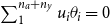 $\sum_1^{n_a+n_y} u_i\theta_i= 0$
where
 $u_i,\, i = 1,\ldots, n_a+n_y$
, are realisations of independent uniform variables on [0, 1], i.e.,
 $\mathcal{U}(0,1)$
. Let
 $\hat {\boldsymbol{\theta}}_s$
and
 $\hat {\boldsymbol{\theta}}_r$
be the estimates of
 $\boldsymbol{\theta}$
under the two systems. Then, by our fundamental result (2),
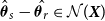 $\hat {\boldsymbol{\theta}}_s - \hat {\boldsymbol{\theta}_r} \in \mathcal{N}(\textbf{\textit{X}})$
and so
 \begin{equation} \hat {\boldsymbol{\theta}}_s - \hat {\boldsymbol{\theta}}_r = A\left(\begin{array}{c} \phantom{-}\textbf{1}_{n_a} \\[6pt] - \textbf{1}_{n_y}\end{array}\right)\end{equation}
for some scalar A. Equating coefficients, we find that
 \begin{equation}\hat {\boldsymbol{\alpha}}_s - \hat {\boldsymbol{\alpha}}_r = A \textbf{1}_{n_a}, \quad \hat {\boldsymbol{\kappa}}_s - \hat {\boldsymbol{\kappa}}_r = - A \textbf{1}_{n_y}\end{equation}
where  $\hat {\boldsymbol{\alpha}}_s$
,
 $\hat {\boldsymbol{\kappa}}_s$
,
 $\hat {\boldsymbol{\alpha}}_r$
and
 $\hat {\boldsymbol{\kappa}}_r$
are the components of
 $\hat{\boldsymbol{\theta}}_s$
and
 $\hat {\boldsymbol{\theta}_r}$
, respectively. The value of A depends on the particular values of
 $u_i$
; in our computation, we found
 $A = 20.7$
although any value of A is possible since it corresponds to adding A to
 $\alpha_x$
and subtracting A from
 $\kappa_y$
in (16). We note that (20) confirms what has been widely observed, namely that the
 $\boldsymbol{\alpha}$
and
 $\boldsymbol{\kappa}$
are only estimable up to an additive constant. A careful discussion of what can and cannot be estimated in the AP model can be found in Clayton & Schifflers (Reference Clayton and Schifflers1987a).
Forecasting in the AP model is done by forecasting the  $\boldsymbol{\kappa}$
values, keeping the
 $\boldsymbol{\alpha}$
values fixed at their estimated values and then using equation (16) to forecast the values of
 $\log \mu$
at each age. Informally, we argue that since
 $\hat {\boldsymbol{\kappa}}_s$
and
 $\hat {\boldsymbol{\kappa}}_r$
are parallel with
 $\hat {\boldsymbol{\kappa}}_s - \hat {\boldsymbol{\kappa}}_r = - A \textbf{1}_{n_y}$
, we require that their forecast values,
 $\hat {\boldsymbol{\kappa}}_{s, f}$
and
 $\hat {\boldsymbol{\kappa}}_{r, s}$
say, are also parallel with
 $\hat {\boldsymbol{\kappa}}_{s, f} - \hat {\boldsymbol{\kappa}}_{r, f} = - A \textbf{1}_{n_f}$
, where
 $n_f$
is the length of the forecast. Now, the forecast values under both constraint systems will be equal since the change in the
 $\boldsymbol{\kappa}$
forecast values is exactly compensated for by the change in the
 $\boldsymbol{\alpha}$
values. This will be achieved with an ARIMA
 $(p, \delta, q)$
model,
 $\delta = 1$
or 2, since the fitted means of the forecasts for
 $\hat {\boldsymbol{\kappa}}_s$
and
 $\hat {\boldsymbol{\kappa}}_r$
will differ by
 $-A$
.
This informal argument extends to the case when  $\hat {\boldsymbol{\kappa}}_s$
and
 $\hat {\boldsymbol{\kappa}}_r$
differ by a linear function, as is the case in the age-period-cohort model for example. Here, we want the forecasts to obey the same linear relationship. A formal argument is given in section 4.3.2 when we discuss the age-period-cohort-improvements model.
We make the important remark that not all forecasting models used in the forecasting of mortality lead to forecasts which are invariant with respect to the choice of constraints. For example, if we forecast  $\boldsymbol{\kappa}$
with an AR(1) model without a mean, then the forecasts will not be invariant. In this paper, we take the position that if two time series differ by a function, then the forecasts should differ by the same function. For example, in the AP model,
 $\hat {\boldsymbol{\kappa}}_s$
and
 $\hat {\boldsymbol{\kappa}}_r$
differ by a constant function, i.e., are parallel; our forecasts should also be parallel. In the APC model, estimates of the period terms and of the cohort terms differ by linear functions. Again, we want our forecasts of the period and cohort terms to obey the same functional relationship. In this way, we will find that not only are fitted values of mortality invariant with respect to the choice of constraints so also are their forecast values.
4.1.2 Smooth AP model
We turn now to the effect of constraints when some model terms are smoothed. In the AP model, the forecast values of  $\log \boldsymbol{\mu}$
are more regular by age if the age parameters
 $\boldsymbol{\alpha}$
are smoothed (see Delwarde et al., Reference Delwarde, Denuit and Eilers2007; Currie, Reference Currie2013). Let
 $\boldsymbol{\alpha} =\textbf{\textit{B}}_a \textbf{\textit{a}}$
, where
 $\textbf{\textit{B}}_a$
is a B-spline regression matrix along age; here,
 $\textbf{\textit{B}}_a$
is
 $n_a \times c_a$
, where
 $c_a$
is the number of B-splines in the basis. The model matrix (17) becomes
 \begin{equation} \textbf{\textit{X}} = [\textbf{\textit{X}}_a\,{:}\,\textbf{\textit{X}}_y] = [\textbf{1}_{n_y} \otimes \textbf{\textit{B}}_a\,{:}\,\textbf{\textit{I}}_{n_y} \otimes \textbf{1}_{n_a}],\; n_a\,n_y \times (c_a+n_y)\end{equation}
with rank  $c_a+n_y-1$
; the regression coefficients
 $\boldsymbol{\theta} =(\textbf{\textit{a}}^\prime, \boldsymbol{\kappa}^\prime)^\prime$
. We distinguish between the regression coefficients denoted
 $\boldsymbol{\theta}$
and the parameters of interest which we denote
 $\boldsymbol{\theta}^*$
; here
 $\boldsymbol{\theta}^* = (\boldsymbol{\alpha}^\prime, \boldsymbol{\kappa}^\prime)^\prime$
. Let
 $\textbf{\textit{X}}^*$
be the model matrix (17) in the unsmoothed case. We note that
 \begin{equation}\textbf{\textit{X}} \boldsymbol{\theta} = \textbf{\textit{X}}^* \boldsymbol{\theta}^*\end{equation}
since  $(\textbf{1}_{n_y} \otimes \textbf{\textit{B}}_a) \textbf{\textit{a}} = (\textbf{1}_{n_y} \otimes \textbf{\textit{I}}_{n_a}) \boldsymbol{\alpha}$
. We will see that (22) is a very convenient identity. If there is no smoothing then
 $\boldsymbol{\theta} = \boldsymbol{\theta}^*$
and
 $\textbf{\textit{X}} = \textbf{\textit{X}}^*$
.
The penalty matrix is
 \begin{equation*} \textbf{\textit{P}} = \mbox{blockdiag}\{\lambda_a \textbf{\textit{D}}^\prime \textbf{\textit{D}}, \textbf{0}\}\end{equation*}
where  $\textbf{\textit{D}}$
is the difference matrix of order d acting on the smoothed age coefficients
 $\textbf{\textit{a}}$
,
 $\textbf{0}$
is the
 $n_y \times n_y$
matrix of 0s acting on the unsmoothed year coefficients
 $\boldsymbol{\kappa}$
and
 $\lambda_a$
is the smoothing parameter. We compute
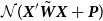 $\mathcal{N}(\textbf{\textit{X}}^\prime \tilde {\textbf{\textit{W}}} \textbf{\textit{X}} +\textbf{\textit{P}})$
for the model in equation (21). Let
 \begin{equation*} \textbf{\textit{n}} = \left(\begin{array}{c} \phantom{-}\textbf{1}_{c_a} \\[6pt] - \textbf{1}_{n_y}\end{array}\right)\end{equation*}
Using the fact that  $\textbf{\textit{B}}_a \textbf{1}_{c_a} = \textbf{1}_{n_a}$
, we see that
 $\textbf{\textit{X}} \textbf{\textit{n}} = \textbf{0}$
, i.e.,
 $\textbf{\textit{n}} \in \mathcal{N}(\textbf{\textit{X}})$
. Furthermore, we have
 $\textbf{\textit{D}} \textbf{1}_{c_a} = \textbf{0}$
for any order
 $d > 0$
of the penalty; hence,
 $\textbf{\textit{P}} \textbf{\textit{n}} = \textbf{0}$
, i.e.,
 $\textbf{\textit{n}} \in \mathcal{N}(\textbf{\textit{P}})$
. Hence, by (13),
 $\mathcal{N}(\textbf{\textit{X}}^\prime \tilde {\textbf{\textit{W}}} \textbf{\textit{X}}+ \textbf{\textit{P}}) = \mathcal{N}(\textbf{\textit{X}}^\prime \tilde {\textbf{\textit{W}}} \textbf{\textit{X}}) \cap \mathcal{N}(\textbf{\textit{P}}) = \textbf{\textit{n}}$
. Thus, if
 $\hat {\boldsymbol{\theta}_s}$
and
 $\hat {\boldsymbol{\theta}_r}$
are any two estimates of
 $\boldsymbol{\theta}$
, we have
 \begin{equation*} \hat {\boldsymbol{\theta}_s} - \hat {\boldsymbol{\theta}_r} = A \left(\begin{array}{c} \phantom{-}\textbf{1}_{c_a} \\[6pt] - \textbf{1}_{n_y}\end{array}\right)\end{equation*}
for some scalar A. Pre-multiplying both sides by  $\mbox{blockdiag}\{\textbf{\textit{B}}_a\,{:}\,\textbf{\textit{I}}_{n_y}\}$
, we find
 \begin{equation*} \left(\begin{array}{c} \hat {\boldsymbol{\alpha}}_s \\[6pt] \hat {\boldsymbol{\kappa}}_s\end{array}\right)- \left(\begin{array}{c} \hat {\boldsymbol{\alpha}}_r \\[6pt] \hat {\boldsymbol{\kappa}}_r\end{array}\right) = A \left(\begin{array}{c} \phantom{-}\textbf{1}_{n_a} \\[6pt] - \textbf{1}_{n_y}\end{array}\right)\end{equation*}
exactly as in the unsmoothed case. We conclude that smoothing has no effect on our invariance results for the AP model.
We have presented a mathematical discussion of the AP model. An important practical point is that from a computational point of view, we do not need the detailed understanding provided by this discussion. We can find the rank and effective rank and check the invariance of the fitted and forecast values easily in R (or other computational tool). We will make further comments on the computational aspects of this work as we go.
4.2 Age-period-cohort model
The age-period-cohort or APC model with almost twice as many parameters as the simple AP model gives a much improved fit.
4.2.1 APC model
Under the APC model, we have
 \begin{equation} \log \mu_{x, y} = \alpha_x + \kappa_y + \gamma_{c(x, y)},\; x = 1,\ldots, n_a,\; y = 1,\ldots, n_y \end{equation}
where c(x, y) is the cohort index for age x in year y; with our notation, we have  $c(x, y) = n_a - x + y$
. First, we write model (23) in the standard form (1) and compute its rank. Let
 $\boldsymbol{\theta} = (\boldsymbol{\alpha}^\prime,\boldsymbol{\kappa}^\prime, \boldsymbol{\gamma}^\prime)^\prime$
. The model matrix is
 \begin{equation} \textbf{\textit{X}} = [\textbf{\textit{X}}_a\, :\, \textbf{\textit{X}}_y \, :\, \textbf{\textit{X}}_c],\; n_a\,n_y \times (2n_a+2n_y-1)\end{equation}
where  $\textbf{\textit{X}}_a$
and
 $\textbf{\textit{X}}_y$
are defined in (17); the row of
 $\textbf{\textit{X}}_c$
corresponding to age x and year y contains a one in column
 $n_a-x+y$
and zeros elsewhere. The rank of
 $\textbf{\textit{X}}$
is
 $2n_a+2n_y-4$
and so the dimension of
 $\mathcal{N}(\textbf{\textit{X}})$
is three. The relationship between the estimates of
 $\boldsymbol{\theta}$
under different constraint systems is determined by
 $\mathcal{N}(\textbf{\textit{X}})$
.
We now find a basis  $\{\textbf{\textit{n}}_1, \textbf{\textit{n}}_2, \textbf{\textit{n}}_3\}$
for
 $\mathcal{N}(\textbf{\textit{X}})$
. We note that this basis is not unique, but we can find a basis that clarifies the relationship between the different estimates of
 $\boldsymbol{\theta}$
. First, we argue that each of
 $\textbf{\textit{X}}_a$
,
 $\textbf{\textit{X}}_y$
and
 $\textbf{\textit{X}}_c$
contains a one in each row and zeros elsewhere. Hence, we can take
 $\textbf{\textit{n}}_1$
and
 $\textbf{\textit{n}}_2$
equal to
 \begin{equation} \textbf{\textit{n}}_1 = \left(\begin{array}{c} \phantom{-} \textbf{1}_{n_a} \\[6pt] - \textbf{1}_{n_y} \\[6pt] \phantom{-} \textbf{0}_{n_c}\end{array}\right), \quad \textbf{\textit{n}}_2 = \left(\begin{array}{c} \phantom{-} \textbf{1}_{n_a} \\[6pt] \phantom{-} \textbf{0}_{n_y} \\[6pt] - \textbf{1}_{n_c}\end{array}\right)\end{equation}
It remains to find a suitable  $\textbf{\textit{n}}_3$
. Some computation is helpful. We fit the APC model under a set of standard constraints, which we take as
 \begin{equation} \sum_1^{n_y} \kappa_y = \sum_1^{n_c} \gamma_c = \sum_1^{n_c}c \gamma_c = 0\end{equation}
where c is the cohort index (Cairns et al., Reference Cairns, Blake, Dowd, Coughlan, Epstein, Ong and Balevich2009). An alternative is to weight by the number of times cohort c appears in the data, say,  $w_c$
. Thus, we could use
 \begin{equation*} \sum_1^{n_y} \kappa_y = \sum_1^{n_c} w_c \gamma_c = \sum_1^{n_c}w_c c \gamma_c = 0\end{equation*}
as in Richards et al. (to appear). Our main point is that, although we will get (slightly) different parameter estimates with these constraint systems, our forecasts of mortality will be identical. We also fit the model with a set of random constraints
 \begin{align*} \sum u_{i, j} \theta_j = 0,\;i = 1,2,3,\; j = 1,\ldots, n_a+n_y+n_c\end{align*}
where the  $u_{i, j}$
are independent realisations from the
 $\mathcal{U}(0,1)$
distribution. Let
 $\hat {\boldsymbol{\theta}}_s$
and
 $\hat {\boldsymbol{\theta}}_r$
be the maximum likelihood estimates of
 $\boldsymbol{\theta}$
under the two constraint systems. Let
 $\hat {\boldsymbol{\alpha}}_s$
,
 $\hat {\boldsymbol{\kappa}}_s$
and
 $\hat {\boldsymbol{\gamma}}_s$
be the components of
 $\hat {\boldsymbol{\theta}}_s$
with a corresponding notation for the components of
 $\hat{\boldsymbol{\theta}}_r$
. The null space of
 $\textbf{\textit{X}}$
characterises
 $\hat {\boldsymbol{\theta}}_s - \hat {\boldsymbol{\theta}}_r$
, so we define
 \begin{equation} \Delta \hat {\boldsymbol{\alpha}} = \hat {\boldsymbol{\alpha}}_s - \hat {\boldsymbol{\alpha}}_r, \; \Delta \hat {\boldsymbol{\kappa}} = \hat {\boldsymbol{\kappa}}_s - \hat {\boldsymbol{\kappa}}_r, \; \Delta \hat {\boldsymbol{\gamma}} = \hat {\boldsymbol{\gamma}}_s - \hat {\boldsymbol{\gamma}}_r\end{equation}
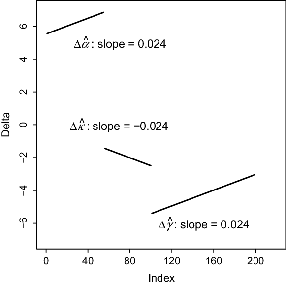
Figure 2 is a plot of  $\Delta \hat {\boldsymbol{\alpha}}$
,
 $\Delta \hat {\boldsymbol{\kappa}}$
and
 $\Delta \hat {\boldsymbol{\gamma}}$
and suggests that these values are linear with slopes C,
 $-C$
and C, respectively, for some C. Thus,
 \begin{eqnarray*} \hat {\boldsymbol{\alpha}}_s - \hat {\boldsymbol{\alpha}}_r &=& a \textbf{1}_{n_a} + b \textbf{\textit{x}}_a \\ \hat {\boldsymbol{\kappa}}_s - \hat {\boldsymbol{\kappa}}_r &=& c \textbf{1}_{n_y} - b \textbf{\textit{x}}_y \\ \hat {\boldsymbol{\gamma}}_s - \hat {\boldsymbol{\gamma}}_r &=& d \textbf{1}_{n_c} + b \textbf{\textit{x}}_c\end{eqnarray*}
for some a, b, c and d. Since  $\textbf{\textit{n}}_3$
is defined only up to scale, we may take
 $b = 1$
and conjecture that
 $\textbf{\textit{n}}_3$
has the form
 \begin{equation} \textbf{\textit{n}}_3 = \left(\begin{array}{c} a \textbf{1}_{n_a} + \textbf{\textit{x}}_a \\[6pt] c \textbf{1}_{n_y} - \textbf{\textit{x}}_y \\[6pt] d \textbf{1}_{n_c} + \textbf{\textit{x}}_c\end{array}\right)\end{equation}
Let  $\textbf{\textit{x}}^\prime_1$
be the first row of
 $\textbf{\textit{X}}$
; we require
 $\textbf{\textit{x}}^\prime_1 \textbf{\textit{n}}_3 = 0$
. We have
 \begin{equation} \textbf{\textit{x}}^\prime_1 \textbf{\textit{n}}_3 = (a+1) + (c-1) + (d+n_a) = a + c + d + n_a = 0\end{equation}
Here, and subsequently, brackets used in this way indicate the terms for age, year and cohort, respectively, and help to clarify the argument. Any solution of (29) will do. A convenient choice is  $a = c = 0$
and
 $d = -n_a$
; our candidate
 $\textbf{\textit{n}}_3$
is
 \begin{equation} \textbf{\textit{n}}_3 = \left(\begin{array}{c} \phantom{-} \textbf{\textit{x}}_a \\[6pt] - \textbf{\textit{x}}_y \\[6pt] \textbf{\textit{x}}_c - n_a \textbf{1}_{n_c}\end{array}\right)\end{equation}
We check that  $\textbf{\textit{X}} \textbf{\textit{n}}_3 = \textbf{0}$
and conclude that
 $\{\textbf{\textit{n}}_1, \textbf{\textit{n}}_2, \textbf{\textit{n}}_3\}$
is a basis for
 $\mathcal{N}(\textbf{\textit{X}})$
, where
 $\textbf{\textit{n}}_1$
and
 $\textbf{\textit{n}}_2$
are defined in (25), and
 $\textbf{\textit{n}}_3$
in (30). Our estimates
 $\hat {\boldsymbol{\theta}}_s$
and
 $\hat {\boldsymbol{\theta}}_r$
then satisfy
 \begin{equation} \hat {\boldsymbol{\theta}}_s - \hat {\boldsymbol{\theta}}_r =A\left(\begin{array}{c} \phantom{-} \textbf{1}_{n_a} \\[6pt] - \textbf{1}_{n_y} \\[6pt] \phantom{-} \textbf{0}_{n_c}\end{array}\right) +B \left(\begin{array}{c} \phantom{-} \textbf{1}_{n_a} \\[6pt] \phantom{-} \textbf{0}_{n_y} \\[6pt] - \textbf{1}_{n_c}\end{array}\right) +C\left(\begin{array}{c} \phantom{-}\textbf{\textit{x}}_a \\[6pt] - \textbf{\textit{x}}_y \\[6pt] \textbf{\textit{x}}_c -n_a \textbf{1}_{n_c}\end{array}\right)\end{equation}
for some scalars A, B and C; in our example, we found  $A =1.42$
,
 $B = 4.10$
and
 $C = 0.024$
. We note that (31) confirms what is widely known, namely that the age, period and cohort parameters are only estimable up to linear functions; see for example, Cairns et al. (Reference Cairns, Blake, Dowd, Coughlan, Epstein, Ong and Balevich2009).



We use the relationships (31) to investigate forecasting with the APC model. We suppose we forecast with an autoregressive integrated moving average model ARIMA $(p, \delta, q)$
. We know from (31) that both
 $\hat {\boldsymbol{\kappa}}_s$
and
 $\hat {\boldsymbol{\kappa}}_r$
, and
 $\hat {\boldsymbol{\gamma}}_s$
and
 $\hat {\boldsymbol{\gamma}}_r$
differ by linear functions. We consider two cases: (a) forecasting the cohort effects with a simple random walk and (b) models with
 $\delta= 1$
or 2.
Case (a): Forecasting $\hat{\boldsymbol{\gamma}}$
with a simple random walk.
The constraints (26) imply that fitted values of  $\boldsymbol{\gamma}$
have mean and slope of zero, and hence the simple random walk is a plausible model for forecasting cohort effects. We suppose that both
 $\hat{\boldsymbol{\gamma}}_s$
and
 $\hat{\boldsymbol{\gamma}}_r$
are forecast in this way. Then a straightforward computation shows that the resulting forecasts of mortality are not equal, i.e., are not invariant with respect to the choice of constraints. The reason for this is that the forecasts of
 $\hat{\boldsymbol{\gamma}}_s$
and
 $\hat{\boldsymbol{\gamma}}_r$
are now parallel and the linear relationship between
 $\hat{\boldsymbol{\gamma}}_s$
and
 $\hat{\boldsymbol{\gamma}}_r$
in (31) has been broken.
We can use a simple device to illustrate further forecasting cohort effects with a simple random walk. If we fit an ARIMA(0,1,0) model, i.e., a random walk with drift, to  $\hat{\boldsymbol{\gamma}}_s$
, then the estimate of the drift parameter,
 $\mu_s$
say, is
 \begin{equation} \hat \mu_s = {\hat {\gamma_s}(n_c) - \hat {\gamma_s}(1) \over n_c -1}\end{equation}
We replace the standard constraints in (26) with
 \begin{equation} \sum_1^{n_y} \kappa_y = \sum_1^{n_c} \gamma_c = \gamma_{n_c} - \gamma_1 = 0\end{equation}
We suppose the resulting estimates are denoted  $\hat{\boldsymbol{\alpha}}_z$
 $\hat{\boldsymbol{\kappa}}_z$
and
 $\hat{\boldsymbol{\gamma}}_z$
. Now when we fit the ARIMA(0,1,0) model to
 $\hat{\boldsymbol{\gamma}}_z$
, the estimate of the drift parameter is constrained to be zero by (33), i.e., we have fitted a simple random walk. We must forecast
 $\hat{\boldsymbol{\gamma}}_s$
with the same ARIMA(0,1,0) model; here, the estimate of the drift parameter is not zero, but the forecasts of mortality under both constraint systems are equal.
Case (b): Forecasting with an ARIMA( $p, \delta, q$
) model,
 $\delta = 1,2$
.
We know from (31) that
 \begin{equation} \hat {\boldsymbol{\kappa}}_s - \hat {\boldsymbol{\kappa}}_r = -A\textbf{1}_{n_y} - C\textbf{\textit{x}}_y\end{equation}
Thus  $\hat {\boldsymbol{\kappa}}_s$
and
 $\hat {\boldsymbol{\kappa}}_r$
differ by a linear function. We should expect that any reasonable forecasts of
 $\hat {\boldsymbol{\kappa}}_s$
and
 $\hat {\boldsymbol{\kappa}}_r$
obey the same functional relation. We show that this is indeed the case when an ARIMA(
 $p, \delta, q$
) model with a mean,
 $\delta = 1,2$
, is used to forecast. A formal proof of this is given in Appendix C. In summary, we will only consider forecasting models that obey this functional relationship since, as we shall see, this will preserve the invariance of forecasts with respect to the choice of constraints.
Let  $\hat {\boldsymbol{\kappa}}_{s, f}$
and
 $\hat {\boldsymbol{\kappa}}_{r, f}$
denote the forecast values of
 $\hat {\boldsymbol{\kappa}}_s$
and
 $\hat {\boldsymbol{\kappa}}_r$
, respectively. It follows from (34) and (C.5) in Appendix C with
 $a = -A$
and
 $b = -C$
that
 \begin{equation} \hat {\boldsymbol{\kappa}}_{s, f} -\hat {\boldsymbol{\kappa}}_{r, f} = -(A + n_yC) \textbf{1}_{n_f} - C \textbf{\textit{x}}_f\end{equation}
where  $\textbf{\textit{x}}_f = (1,\ldots, n_f)^\prime$
. The analogous argument with
 $\hat {\boldsymbol{\gamma}}_s - \hat {\boldsymbol{\gamma}}_r$
shows that
 \begin{equation} \hat {\boldsymbol{\gamma}}_{s, f} -\hat {\boldsymbol{\gamma}}_{r, f} = -(B + (n_y-1)C) \textbf{1}_{n_f} + C \textbf{\textit{x}}_f\end{equation}
where  $\hat {\boldsymbol{\gamma}}_{s, f}$
and
 $\hat {\boldsymbol{\gamma}}_{r, f}$
are the forecast values of
 $\hat {\boldsymbol{\gamma}}_s$
and
 $\hat {\boldsymbol{\gamma}}_r$
, respectively.
We can now establish the invariance of the forecast values of  $\log\mu$
. Define
 \begin{equation*} \hat{ \boldsymbol{\theta}}_{s, f} = (\hat{\boldsymbol{\alpha}}_s^\prime, \hat{\boldsymbol{\kappa}}_s^\prime, \hat{\boldsymbol{\kappa}}_{s, f}^\prime, \hat{\boldsymbol{\gamma}}_s^\prime, \hat{\boldsymbol{\gamma}}_{s, f}^\prime)^\prime\end{equation*}
with a similar definition for  $\hat{ \boldsymbol{\theta}}_{r, f}$
. Let
 $\textbf{\textit{X}}_f$
be the model matrix for the APC model for ages
 $\textbf{\textit{x}}_a$
and years
 $(\textbf{\textit{x}}_y^\prime, \textbf{\textit{x}}_{y, f}^\prime)^\prime$
, where
 $\textbf{\textit{x}}_{y, f} =(n_y + 1, \ldots, n_y + n_f)^\prime$
. We can show that
 $\textbf{\textit{X}}_f(\hat{ \boldsymbol{\theta}}_{s, f} -\hat{ \boldsymbol{\theta}}_{r, f}) = \textbf{0}$
. We omit the proof and instead give a detailed proof in the next section for a smooth version of the APCI model; the present case follows in the same fashion. We can therefore conclude that the fitted and forecast values of mortality in the APC model are invariant with respect to the choice of constraints when an ARIMA
 $(p, \delta, q)$
model,
 $\delta =1$
or 2, with a mean is used to forecast.
A “computer proof” of the above result is simple and for many models of mortality is all that is reasonably available or indeed required. We compute fitted and forecast values under any two constraint systems and check the invariance of the fitted and forecast values. Once the basic code is written, different constraint systems and different forecasting regimes are easily applied. We have used this approach in parallel with our theoretical discussion.
4.2.2 Smooth APC model
Just as in the AP model, forecasting of mortality in the APC model is improved if the age parameters  $\boldsymbol{\alpha}$
are smoothed. We set
 $\boldsymbol{\alpha} = \textbf{\textit{B}}_a \textbf{\textit{a}}$
, where
 $\textbf{\textit{B}}_a$
is
 $n_a \times c_a$
, and replace
 $\textbf{\textit{X}}_a$
in (24) with
 $\textbf{1}_{n_y} \otimes \textbf{\textit{B}}_a$
, as in (21). The model matrix becomes
 \begin{equation} \textbf{\textit{X}} = [\textbf{1}_{n_y} \otimes \textbf{\textit{B}}_a\,{:}\,\textbf{\textit{I}}_{n_y} \otimes \textbf{1}_{n_a}\,{:}\,\textbf{\textit{X}}_c],\; n_an_y \times (c_a+n_a+2n_y-1)\end{equation}
and the penalty matrix is
 \begin{equation} \textbf{\textit{P}} = \mbox{blockdiag}\{\lambda_a \textbf{\textit{D}}^\prime \textbf{\textit{D}}, \textbf{0}\}\end{equation}
where  $\textbf{\textit{D}}$
is the difference matrix of order d acting on the smoothed age coefficients
 $\textbf{\textit{a}}$
,
 $\textbf{0}$
is the
 $(n_y+n_c) \times(n_y+n_c)$
matrix of 0s acting on the unsmoothed year and cohort coefficients
 $\boldsymbol{\kappa}$
and
 $\boldsymbol{\gamma}$
, and
 $\lambda_a$
is the smoothing parameter. With the P-spline system, it is usual to smooth with a second-order penalty. However, if a first-order penalty is used, we find the effective rank of the model is increased by one; in this case, in order to retain invariance the number of constraints should be reduced to two. We continue with a detailed discussion of the case when a second-order penalty is used.
The regression parameter is  $\boldsymbol{\theta} = (\textbf{\textit{a}}^\prime, \boldsymbol{\kappa}^\prime, \boldsymbol{\gamma}^\prime)^\prime$
. It is easy to see that
 \begin{equation} \textbf{\textit{n}}_1 = \left(\begin{array}{c} \phantom{-}\textbf{1}_{c_a} \\[6pt] -\textbf{1}_{n_y} \\[6pt]
\phantom{-}\textbf{0}_{n_c} \end{array}\right), \quad \textbf{\textit{n}}_2 = \left(\begin{array}{c} \phantom{-}\textbf{1}_{c_a} \\[6pt] \phantom{-}\textbf{0}_{n_y} \\[6pt] -\textbf{1}_{n_c} \end{array}\right)\end{equation}
are in  $\mathcal{N}(\textbf{\textit{X}})$
. We use an extension of the argument used in the unsmoothed case to find a suitable third basis vector,
 $\textbf{\textit{n}}_3$
. We fit with the standard constraints (26) and also with some random constraints but with
 $\lambda_a = 0$
(since we are interested in determining a basis for
 $\mathcal{N}(\textbf{\textit{X}})$
). Corresponding to (27), we define
 \begin{equation} \Delta \hat {\textbf{\textit{a}}} = \hat {\textbf{\textit{a}}}_s - \hat {\textbf{\textit{a}}}_r, \; \Delta \hat {\boldsymbol{\kappa}} = \hat {\boldsymbol{\kappa}}_s - \hat {\boldsymbol{\kappa}}_r, \; \Delta \hat {\boldsymbol{\gamma}} = \hat {\boldsymbol{\gamma}}_s - \hat {\boldsymbol{\gamma}}_r\end{equation}
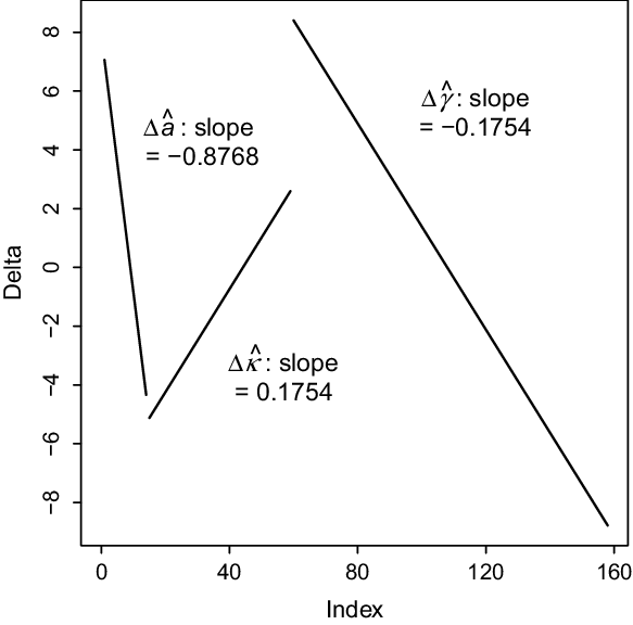
In our example, we used a knot spacing of  $\Delta_a = 5$
. From Figure 3, we note that
 $\Delta \hat {\boldsymbol{\kappa}}$
and
 $\Delta \hat {\boldsymbol{\gamma}}$
are linear with slopes 0.1754 and
 $-0.1754$
, respectively, while
 $\Delta \hat {\boldsymbol{\alpha}}$
is linear with slope
 $-0.8768 \approx -\Delta_a 0.1754$
. Hence, as in (28), we conjecture that
 $\textbf{\textit{n}}_3$
has the form
 \begin{equation*} \textbf{\textit{n}}_3 = \left(\begin{array}{c} a \textbf{1}_{c_a} + \Delta_a \textbf{\textit{x}}_{c_a} \\[6pt] c \textbf{1}_{n_y} - \textbf{\textit{x}}_y \\[6pt] d \textbf{1}_{n_c} + \textbf{\textit{x}}_c\end{array}\right)\end{equation*}
where  $\textbf{\textit{x}}_{c_a} = (1,2,3,\ldots, c_a)^\prime$
. Let
 $\textbf{\textit{x}}^\prime_1$
be the first row of
 $\textbf{\textit{X}}$
; we set
 $\textbf{\textit{x}}^\prime_1 \textbf{\textit{n}}_3 = 0$
. We recall that in the computation of
 $\textbf{\textit{B}}_a$
, we place a knot at the first age. With this assumption, the first row of
 $\textbf{\textit{B}}_a$
is
 $(\frac{1}{6},\frac{2}{3},\frac{1}{6}, {\boldsymbol{0}}^{\prime}_{c_{a}-3})$
. We have
 \begin{equation*} \textbf{\textit{x}}^\prime_1 \textbf{\textit{n}}_3 = \left(a+\Delta_a\!\left(\mbox{${1\over6}$} + \mbox{${4\over3}$} + \mbox{${3\over6}$}\right)\right) + (c-1) + (d+n_a) = a + c + d + n_a + 2\Delta_a - 1 = 0.\end{equation*}
A convenient solution is  $a = c = 0$
and
 $d = 1 - n_a - 2\Delta_a$
; our candidate
 $\textbf{\textit{n}}_3$
is
 \begin{equation} \textbf{\textit{n}}_3 = \left(\begin{array}{c} \Delta_a \textbf{\textit{x}}_{c_a} \\[6pt] - \textbf{\textit{x}}_y \\[6pt] \textbf{\textit{x}}_c - \omega_c \textbf{1}_{n_c}\end{array}\right)\end{equation}
where  $\omega_c = -d = n_a + 2\Delta_a -1$
. We now check that
 $\textbf{\textit{X}} \textbf{\textit{n}}_3 = \textbf{0}$
. We conclude that
 $\{\textbf{\textit{n}}_1, \textbf{\textit{n}}_2, \textbf{\textit{n}}_3\}$
is a basis for
 $\mathcal{N}(\textbf{\textit{X}})$
, where
 $\textbf{\textit{n}}_1$
and
 $\textbf{\textit{n}}_2$
are defined in (39) and
 $\textbf{\textit{n}}_3$
in (41). Hence,
 \begin{equation}\hat {\boldsymbol{\theta}}_s - \hat {\boldsymbol{\theta}}_r = A \left(\begin{array}{c} \phantom{-}\textbf{1}_{c_a} \\[6pt] -\textbf{1}_{n_y} \\[6pt] \phantom{-}\textbf{0}_{n_c} \end{array}\right) + B \left(\begin{array}{c} \phantom{-}\textbf{1}_{c_a} \\[6pt] \phantom{-}\textbf{0}_{n_y} \\[6pt] -\textbf{1}_{n_c} \end{array}\right) + C \left(\begin{array}{c} \Delta_a \textbf{\textit{x}}_{c_a} \\[6pt] -\textbf{\textit{x}}_y \\[6pt] \textbf{\textit{x}}_c - \omega_c \textbf{1}_{n_c} \end{array}\right)\end{equation}
for some A, B and C; in our example, we found  $A = 5.298$
,
 $B =2.644$
and
 $C = -0.1754$
. Pre-multiplying (42) through by
 $\mbox{blockdiag}\{\textbf{\textit{B}}_a, \textbf{\textit{I}}_{n_y}, \textbf{\textit{I}}_{n_c}\}$
and using
 $\textbf{\textit{B}}_a \textbf{1}_{c_a} = \textbf{1}_{n_a}$
and
 $\textbf{\textit{B}}_a \Delta_a \textbf{\textit{x}}_{c_a}= \textbf{\textit{x}}_{n_a} + \omega_a \textbf{1}_{n_a}$
,
 $\omega_a = 2\Delta_a - 1$
, we find
 \begin{equation}\begin{array}{c} \phantom{0} \\[6pt] \hat{\boldsymbol{\theta}}_s^* \\[6pt] \phantom{0}\end{array} -\begin{array}{c} \phantom{0} \\[6pt] \hat{\boldsymbol{\theta}}_r^* \\[6pt] \phantom{0}\end{array} =A \left(\begin{array}{c} \phantom{-}\textbf{1}_{n_a} \\[6pt] -\textbf{1}_{n_y} \\[6pt] \phantom{-}\textbf{0}_{n_c} \end{array}\right) + B \left(\begin{array}{c} \phantom{-}\textbf{1}_{n_a} \\[6pt] \phantom{-}\textbf{0}_{n_y} \\[6pt] -\textbf{1}_{n_c} \end{array}\right) + C \left(\begin{array}{c} \textbf{\textit{x}}_a + \omega_a \textbf{1}_{n_a} \\[6pt] -\textbf{\textit{x}}_y \\[6pt] \textbf{\textit{x}}_c - \omega_c \textbf{1}_{n_c} \end{array}\right)\end{equation}
where  $\boldsymbol{\theta}^* = (\boldsymbol{\alpha}^\prime, \boldsymbol{\kappa}^\prime, \boldsymbol{\gamma}^\prime)^\prime$
denotes the parameters of interest.




We show that forecasting with an ARIMA( $p, \delta, q)$
,
 $\delta = 1$
or 2, is invariant with respect to the choice of constraints. We use the same notation as in the unsmoothed case. Comparing (31) and (43), we see that the middle rows are identical. Hence, the forecasts of
 $\boldsymbol{\kappa}$
under two different constraint systems in the smoothed case obey the same relation (35) as in the unsmoothed case, i.e.,
 \begin{equation*} \hat {\boldsymbol{\kappa}}_{s, f} - \hat {\boldsymbol{\kappa}}_{r, f} = -(A + n_y C) \textbf{1}_{n_f} - C \textbf{\textit{x}}_f\end{equation*}
Forecasts of  $\boldsymbol{\gamma}$
obey the following
 \begin{eqnarray*} \nonumber \hat {\boldsymbol{\gamma}}_{s, f} - \hat {\boldsymbol{\gamma}}_{r, f} &=& \left(\hat {\boldsymbol{\gamma}}_s(n_y) - \hat {\boldsymbol{\gamma}}_r(n_y)\right) \textbf{1}_{n_f} + C\textbf{\textit{x}}_{n_f} \\ &=& (\!-B +(n_c - \omega_c)C) \textbf{1}_{n_f} + C \textbf{\textit{x}}_{n_f} \quad \mbox{by (\linkref{disp43}{43})} \\ &=& (\!-B +(n_y - 2\Delta_a)C) \textbf{1}_{n_f} + C \textbf{\textit{x}}_{n_f}\end{eqnarray*}
It now follows that  $\textbf{\textit{X}}_f^* (\hat{\boldsymbol{\theta}}_{s, f}^{\raisebox{-3pt}{\hbox{\fontsize{8}{10}\selectfont$\ast$}}} - \hat {\boldsymbol{\theta}}_{r, f}^{{\raisebox{-3pt}{\hbox{\fontsize{8}{10}\selectfont$\ast$}}}}) = \textbf{0}$
, where
 $\textbf{\textit{X}}_f^*$
is the model matrix (24) in the unsmoothed case; the proof is a special case of that given for the smooth APCI model. We have established the invariance of the fitted and forecast values with respect to the choice of constraint system when an ARIMA(
 $p, \delta, q$
) model,
 $\delta =1$
or 2, is used.
4.3 Age-period-cohort-improvements model
The CMI’s age-period-cohort-improvements or APCI model was introduced as an industry standard for the forecasting of mortality (Continuous Mortality Investigation, 2016a, 2016b, 2016c; Richards et al., to appear).
4.3.1 APCI model
The APCI model is
 \begin{equation} \log\,\mu_{x, y} = \alpha_x + \kappa_y + \gamma_{c(x, y)} + \beta_x(\bar y - y),\;x=1,\ldots,n_a,\;y = 1, \ldots, n_y\end{equation}
where 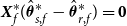 $\bar y = (n_y+1)/2$
(recall the year vector is
 $\textbf{\textit{x}}_y =(1, \ldots, n_y)^\prime$
). We note that (44) differs in a minor way from the CMI’s formulation; we have reversed the sign of the
 $\beta_x$
terms, which now correspond to the
 $\beta_x$
terms in the Lee–Carter model. The thinking behind the APCI model is as follows: linearise the
 $\beta_x \kappa_y$
term in the Lee–Carter model and add the cohort term
 $\gamma_{c(x, y)}$
. This gives a model which takes into account any cohort effects and allows the forecast of the year effect to depend on age. The APCI model is a GLM with model matrix
 \begin{equation} \textbf{\textit{X}} = [\textbf{\textit{X}}_a\, :\, \textbf{\textit{X}}_y \, :\, \textbf{\textit{X}}_c \, :\, \textbf{\textit{X}}_b],\; n_an_y \times (3n_a + 2n_y - 1)\end{equation}
where  $\textbf{\textit{X}}_a$
and
 $\textbf{\textit{X}}_y$
are defined in (17),
 $\textbf{\textit{X}}_c$
in (24) and
 $\textbf{\textit{X}}_b = (\bar y \textbf{1}_{n_y} - \textbf{\textit{x}}_y)\otimes \textbf{\textit{I}}_{n_a}$
. We define
 $\boldsymbol{\theta} = (\boldsymbol{\alpha}^\prime, \boldsymbol{\kappa}^\prime, \boldsymbol{\gamma}^\prime, \boldsymbol{\beta}^\prime)^\prime$
and the model has the form (1). The model matrix has
 $3n_a+ 2n_y - 1$
columns and rank
 $3n_a + 2n_y - 6$
, so five constraints are required to enable
 $\boldsymbol{\theta}$
to be estimated uniquely. The null space of
 $\textbf{\textit{X}}$
is spanned by
 \begin{equation} \left(\begin{array}{c} \phantom{-}\textbf{1}_{n_a} \\[6pt] -\textbf{1}_{n_y} \\[6pt] \phantom{-}\textbf{0}_{n_c} \\[6pt] \phantom{-}\textbf{0}_{n_a} \end{array}\right),\; \left(\begin{array}{c} \phantom{-}\textbf{1}_{n_a} \\[6pt] \phantom{-}\textbf{0}_{n_y} \\[6pt] -\textbf{1}_{n_c} \\[6pt] \phantom{-}\textbf{0}_{n_a} \end{array} \right),\; \left( \begin{array}{c} \phantom{-}\textbf{\textit{x}}_a \\[6pt] -\textbf{\textit{x}}_y \\[6pt] \textbf{\textit{x}}_c - n_a \textbf{1}_{n_c} \\[6pt] \phantom{-} \textbf{0}_{n_a} \end{array} \right),\; \left(\begin{array}{c} \textbf{0}_{n_a} \\[6pt] \textbf{\textit{x}}_y - \bar y \textbf{1}_{n_y} \\[6pt] \textbf{0}_{n_c} \\[6pt] \textbf{1}_{n_a} \end{array} \right),\; \left(\begin{array}{c} Q \textbf{\textit{x}}_a + \textbf{\textit{x}}_a^2 \\[6pt] 2n_a \textbf{\textit{x}}_y + \textbf{\textit{x}}_y^2 \\[6pt] n_a^2 \textbf{1}_{n_c} - \textbf{\textit{x}}_c^2 \\[6pt] 2 \textbf{\textit{x}}_a \end{array}\right)\end{equation}
where  $Q = -2(n_a + \bar y)$
. The first three basis vectors in (46) are the same as the basis vectors for the APC model with
 $\textbf{0}_{n_a}$
appended. The fourth basis vector can be deduced by observing that
 \begin{equation*} \kappa_y + (\bar y - y) \beta_x = \kappa_y - (\bar y - y) \omega + (\bar y - y)(\beta_x + \omega) = \kappa_y^* + (\bar y - y) \beta_x^*\end{equation*}
for any scalar  $\omega$
. The fifth basis vector can be found with the same method as used to find the third basis vector for the APC model. We denote the basis vectors in (46) by
 $\textbf{\textit{n}}_i,\,i=1,\ldots,5$
.
We comment briefly on the CMI’s approach to identifiability. The CMI (2016a, 7.3) gives the following transformation of the parameters which leaves the values of  $\log \boldsymbol{\mu}$
unchanged. We give this transformation in our notation and with the CMI’s
 $\beta_x$
replaced by ours.
 \begin{multline} \nonumber \left(\begin{array}{c} \Delta \alpha_x \\[6pt] \Delta \kappa_y \\[6pt] \Delta \gamma_{y-x} \\[6pt] \Delta \beta_x \end{array}\right)= \theta_1 \left(\begin{array}{c} \phantom{-} 1 \\[6pt] \phantom{-} 0 \\[6pt] -1 \\[6pt] \phantom{-} 0 \end{array}\right)+ \theta_2 \left(\begin{array}{c} - (x - \bar x) \\[6pt] y - \bar y \\[6pt] (x - \bar x) - (y - \bar y) \\[6pt] 0 \end{array}\right)+ \\[6pt] \theta_3 \left(\begin{array}{c} (x - \bar x)^2 \\[6pt] (y - \bar y)^2 \\[6pt] - \left((x - \bar x) - (y - \bar y)\right)^2 \\[6pt] 2(x - \bar x) \end{array}\right) +\theta_4 \left(\begin{array}{c} \phantom{-} 1 \\[6pt] -1 \\[6pt] \phantom{-} 0 \\[6pt] \phantom{-} 0 \end{array}\right)+ \theta_5 \left(\begin{array}{c} 0 \\[6pt] -(y - \bar y) \\[6pt] 0 \\[6pt] (y - \bar y) \end{array}\right)\end{multline}
Writing the transformation in this way, we see that it is equivalent to a particular null basis for  $\textbf{\textit{X}}$
, namely,
 \begin{align} \left(\begin{array}{c} \phantom{-}\textbf{1}_{n_a} \\[6pt] \phantom{-}\textbf{0}_{n_y} \\[6pt] -\textbf{1}_{n_c} \\[6pt] \phantom{-}\textbf{0}_{n_a} \end{array}\right),\; \left( \begin{array}{c} -(\textbf{\textit{x}}_a - \bar a \textbf{1}_{n_a}) \\[6pt] \textbf{\textit{x}}_y - \bar y \textbf{1}_{n_y} \\[6pt] -(\textbf{\textit{x}}_c - \bar c \textbf{1}_{n_c}) \\[6pt] \phantom{-} \textbf{0}_{n_a} \end{array} \right),\; \left(\begin{array}{c} (\textbf{\textit{x}}_a - \bar a \textbf{1}_{n_a})^2 \\[6pt] (\textbf{\textit{x}}_y - \bar y \textbf{1}_{n_y})^2 \\[6pt] -(\textbf{\textit{x}}_c - \bar c \textbf{1}_{n_c})^2 \\[6pt] 2(\textbf{\textit{x}}_a - \bar a \textbf{1}_{n_a}) \end{array} \right),\; \left(\begin{array}{c} \phantom{-}\textbf{1}_{n_a} \\[6pt] -\textbf{1}_{n_y} \\[6pt] \phantom{-} \textbf{0}_{n_c} \\[6pt] \phantom{-}\textbf{0}_{n_a} \end{array} \right),\; \left(\begin{array}{c} \textbf{0}_{n_a} \\[6pt] \textbf{\textit{x}}_y - \bar y \textbf{1}_{n_y} \\[6pt] \textbf{0}_{n_c} \\[6pt] \textbf{1}_{n_a} \end{array}\right)\end{align}
where  $\bar a$
is the mean age,
 $\bar y$
is the mean year and
 $\bar c= n_a - \bar a + \bar y$
. Three of the basis vectors are the same as ours; the other two have the same form. In particular, the third basis vector in (47) has quadratic and linear functions in the equivalent positions to (46).
We fit the model under the standard constraints (CMI, 2016a)
 \begin{equation} \sum \kappa_y = \sum \gamma_c = \sum c \gamma_c = \sum c^2 \gamma_c = \sum y \kappa_y = 0\end{equation}
where c is the cohort index,  $c = 1, \ldots, n_c$
; again, we could use weighted constraints as in Richards et al. (to appear). We also use the random constraints
 \begin{equation} \sum u_{i, j} \theta_j = 0, \, i = 1,\ldots, 5,\, j = 1,\ldots, 3n_a+2n_y -1\end{equation}
where the  $u_{i, j}$
are independent
 $\mathcal{U}(0,1)$
. With our usual notation for the estimates of
 $\boldsymbol{\theta}$
under the standard and random constraints, we have
 \begin{equation*} \hat {\boldsymbol{\theta}}_s - \hat {\boldsymbol{\theta}}_r = A \textbf{\textit{n}}_1 + B \textbf{\textit{n}}_2 + C \textbf{\textit{n}}_3 + D \textbf{\textit{n}}_4 + E \textbf{\textit{n}}_5\end{equation*}
for some A, B, C, D and E. Equating coefficients in (46), we immediately find that  $\hat {\boldsymbol{\alpha}}_s -\hat {\boldsymbol{\alpha}}_r$
,
 $\hat {\boldsymbol{\kappa}}_s - \hat {\boldsymbol{\kappa}}_r$
and
 $\hat {\boldsymbol{\gamma}}_s - \hat {\boldsymbol{\gamma}}_r$
are quadratic functions of
 $\textbf{\textit{x}}_a$
,
 $\textbf{\textit{x}}_y$
and
 $\textbf{\textit{x}}_c$
, respectively, with E, E and
 $-E$
as the coefficients of the quadratic terms; furthermore,
 $\hat {\boldsymbol{\beta}}_s - \hat {\boldsymbol{\beta}}_r$
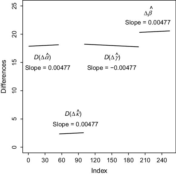
is linear with slope 2E. These relationships have implications for invariance when it comes to forecasting.
Figure 4 confirms the relationships among the coefficients. Since  $\Delta \hat {\boldsymbol{\alpha}} = \hat {\boldsymbol{\alpha}}_s -\hat {\boldsymbol{\alpha}}_r$
is quadratic with the coefficient of the quadratic term equal to E, first differences of
 $\Delta \hat {\boldsymbol{\alpha}}$
,
 $D(\Delta \hat {\boldsymbol{\alpha}})$
, will be linear with slope 2E as shown in Figure 4; the same remark applies to the first differences
 $D(\Delta \hat {\boldsymbol{\kappa}})$
and
 $D(\Delta \hat {\boldsymbol{\gamma}})$
. The slope of
 $\Delta \hat {\boldsymbol{\beta}}$
is 2E. In our example, we found
 $A = -624.3$
,
 $B = -70.02$
,
 $C=18.24$
,
 $D = 20.32$
and
 $E = 0.002385$
.
Plot of first differences, denoted D, of  $\Delta \hat {\boldsymbol{\alpha}} = \hat {\boldsymbol{\alpha}}_s - \hat {\boldsymbol{\alpha}}_r$
,
 $\Delta \hat {\boldsymbol{\kappa}} = \hat {\boldsymbol{\kappa}}_s - \hat {\boldsymbol{\kappa}}_r$
and
 $\Delta \hat {\boldsymbol{\gamma}} = \hat {\boldsymbol{\gamma}}_s - \hat {\boldsymbol{\gamma}}_r$
; plot of
 $\Delta \hat {\boldsymbol{\beta}} = \hat {\boldsymbol{\beta}}_s- \hat {\boldsymbol{\beta}}_r$
in the APCI model (44).

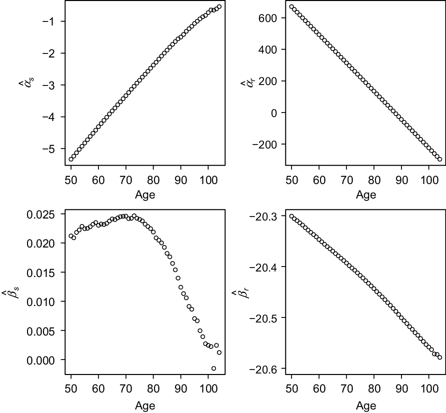
Left: plot of  $\hat {\boldsymbol{\alpha}}_s$
,
 $\hat {\boldsymbol{\beta}}_s$
; right: plot of
 $\hat {\boldsymbol{\alpha}}_r$
and
 $\hat {\boldsymbol{\beta}}_r$
in the APCI model (44).

Figure 5 is a plot of the estimated  $\boldsymbol{\alpha}$
and
 $\boldsymbol{\beta}$
under our two constraint systems; the estimates are wildly different both in shape and range. Under the standard constraint, the estimate of
 $\boldsymbol{\alpha}$
has a familiar look, while the estimate of
 $\boldsymbol{\beta}$
is very close to the estimate of
 $\boldsymbol{\beta}$
in the Lee–Carter model; see Figure 8 for the corresponding plot. However, Figure 5 serves to emphasise our main point: it is how the coefficients join forces that matter, not the individual coefficients themselves.
The CMI smooth both  $\boldsymbol{\alpha}$
and
 $\boldsymbol{\beta}$
in their treatment of the APCI model, and we will focus on this case. First, we discuss briefly the unsmoothed case. We forecast with our two constraint systems, namely standard and random. The quadratic nature of the fifth basis vector in the null space of the APCI model (see (46)) implies that a first-order ARIMA model will not give invariant forecasts. In this paper, we concentrate on forecasting models which lead to invariant forecasts so we do not pursue this further.
4.3.2 Smooth APCI model
The case for smoothing both  $\boldsymbol{\alpha}$
and
 $\boldsymbol{\beta}$
is strong: forecasts will be much less prone to irregular behaviour by age (see Delwarde et al., Reference Delwarde, Denuit and Eilers2007; Currie, Reference Currie2013). We will not smooth either
 $\boldsymbol{\kappa}$
or
 $\boldsymbol{\gamma}$
, since we are interested in stochastic forecasts of these parameters. This is in contrast to the CMI which in addition to smoothing
 $\boldsymbol{\alpha}$
and
 $\boldsymbol{\beta}$
also smooth
 $\boldsymbol{\kappa}$
or
 $\boldsymbol{\gamma}$
; the CMI’s approach is designed to facilitate deterministic targeting of future mortality. We do not comment on this debate here; see Booth & Tickle (Reference Booth and Tickle2008), Richards et al. (to appear).
Let  $\textbf{\textit{B}}_a,\,n_a \times c_a$
, be a regression matrix evaluated over a basis of cubic B-splines for age. We use the same regression matrix to smooth both
 $\boldsymbol{\alpha}$
and
 $\boldsymbol{\beta}$
and set
 $\boldsymbol{\alpha} = \textbf{\textit{B}}_a \textbf{\textit{a}}$
and
 $\boldsymbol{\beta} = \textbf{\textit{B}}_a \textbf{\textit{b}}$
. The model matrix is now
 \begin{equation} \textbf{\textit{X}} = [\textbf{1}_{n_y} \otimes \textbf{\textit{B}}_a\, : \,\textbf{\textit{I}}_{n_y} \otimes \textbf{1}_{n_a}\, : \,\textbf{\textit{X}}_c\, : \,(\bar y \textbf{1}_{n_y} - \textbf{\textit{x}}_y) \otimes \textbf{\textit{B}}_a]\end{equation}
where  $\textbf{\textit{X}}_c$
is defined below (24). The model matrix is
 $n_a\,n_y \times (2c_a + n_y + n_c)$
with
 $r(\textbf{\textit{X}}) = 2c_a + n_y +n_c -5$
, so
 $\mathcal{N}(\textbf{\textit{X}})$
has dimension five. We fit model (50) but without smoothing, i.e., with the smoothing parameters set to zero. Let
 $\boldsymbol{\theta} = (\textbf{\textit{a}}^\prime,\boldsymbol{\kappa}^\prime, \boldsymbol{\gamma}^\prime, \textbf{\textit{b}}^\prime)^\prime$
be the vector of regression coefficients and
 $\boldsymbol{\theta}^* = (\boldsymbol{\alpha}^\prime, \boldsymbol{\kappa}^\prime, \boldsymbol{\gamma}^\prime, \boldsymbol{\beta}^\prime)^\prime$
denote the parameters of interest. We denote the five vectors
 \begin{align} \left(\begin{array}{c} \phantom{-}\textbf{1}_{c_a} \\[6pt] -\textbf{1}_{n_y} \\[6pt] \phantom{-}\textbf{0}_{n_c} \\[6pt] \phantom{-}\textbf{0}_{c_a} \end{array}\right),\; \left(\begin{array}{c} \phantom{-}\textbf{1}_{c_a} \\[6pt] \phantom{-}\textbf{0}_{n_y} \\[6pt] -\textbf{1}_{n_c} \\[6pt] \phantom{-}\textbf{0}_{c_a} \end{array} \right),\; \left( \begin{array}{c} \Delta_a \textbf{\textit{x}}_{c_a} \\[6pt] -\textbf{\textit{x}}_y \\[6pt] \textbf{\textit{x}}_c - \omega_c \textbf{1}_{n_c} \\[6pt] \phantom{-} \textbf{0}_{c_a} \end{array} \right),\; \left(\begin{array}{c} \textbf{0}_{c_a} \\[6pt] \textbf{\textit{x}}_y - \bar y \textbf{1}_{n_y} \\[6pt] \textbf{0}_{n_c} \\[6pt] \textbf{1}_{c_a} \end{array} \right),\; \left(\begin{array}{c} Q_a(\textbf{\textit{x}}_{c_a}) \\[6pt] Q_\kappa(\textbf{\textit{x}}_{n_y}) \\[6pt] Q_\gamma(\textbf{\textit{x}}_{n_c}) \\[6pt] L_b(\textbf{\textit{x}}_{c_a}) \end{array} \right)\end{align}
by  $\textbf{\textit{n}}_1, \ldots,\textbf{\textit{n}}_5$
, respectively; here
 $Q_a(\cdot)$
,
 $Q_\kappa(\cdot)$
and
 $Q_\gamma(\cdot)$
are quadratic functions and
 $L_b(\cdot)$
is a linear function. We can check that
 $\textbf{\textit{n}}_1,\ldots,\textbf{\textit{n}}_4$
are all in
 $\mathcal{N}(\textbf{\textit{X}})$
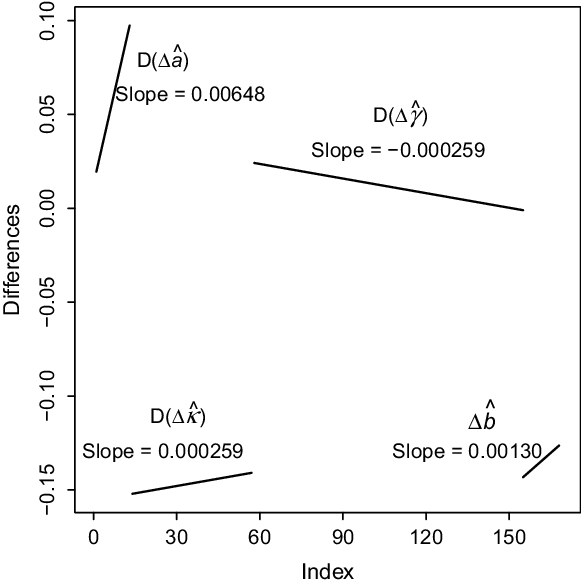
. Figure 6 is a plot of differences in estimates under the standard and random constraints (48) and (49) and suggests that the fifth basis vector in
 $\mathcal{N}(\textbf{\textit{X}})$
has the form
 $\textbf{\textit{n}}_5$
. Additionally, the form of the fifth basis in (46) in the unsmoothed case supports this idea. We will not need an exact expression for
 $\textbf{\textit{n}}_5$
.
Plot of first differences, denoted D, of  $\Delta \hat {\textbf{\textit{a}}} = \hat {\textbf{\textit{a}}}_s - \hat {\textbf{\textit{a}}}_r$
,
 $\Delta \hat {\boldsymbol{\kappa}} = \hat {\boldsymbol{\kappa}}_s - \hat {\boldsymbol{\kappa}}_r$
and
 $\Delta \hat {\boldsymbol{\gamma}} = \hat {\boldsymbol{\gamma}}_s - \hat {\boldsymbol{\gamma}}_r$
; plot of
 $\Delta \hat {\textbf{\textit{b}}} = \hat {\textbf{\textit{b}}}_s - \hat {\textbf{\textit{b}}}_r$
in APCI model with the smooth model matrix (50) but with
 $\lambda_a = \lambda_b = 0$
.

Let  $\textbf{\textit{D}}_a$
and
 $\textbf{\textit{D}}_b$
be difference matrices of orders
 $d_a$
and
 $d_b$
applied to the coefficients
 $\textbf{\textit{a}}$
and
 $\textbf{\textit{b}}$
, respectively. The penalty matrix is
 \begin{equation*} \textbf{\textit{P}} = \mbox{blockdiag}\{\lambda_a \textbf{\textit{D}}_a^\prime \textbf{\textit{D}}_a,\, \textbf{0},\, \lambda_b \textbf{\textit{D}}_b^\prime \textbf{\textit{D}}_b\}\end{equation*}
where  $\textbf{0}$
is a square matrix of 0s of size
 $n_y+n_c$
. The null space of the penalised model is given by
 $\mathcal{N}(\textbf{\textit{X}}) \cap \mathcal{N}(\textbf{\textit{P}})$
; see (13). Now
 $\textbf{\textit{P}} \textbf{\textit{n}}_i = \textbf{0}$
for
 $i = 1,\ldots, 4$
for
 $d_a \ge 2$
and
 $d_b \ge 2$
; for
 $\textbf{\textit{P}} \textbf{\textit{n}}_5 = \textbf{0}$
, we need
 $d_a \ge 3$
and
 $d_b \ge 2$
. It is usual to smooth with difference matrices of order two; in this case
 $\textbf{\textit{n}}_5\notin \mathcal{N}(\textbf{\textit{P}})$
. We continue with the case
 $d_a = d_b = 2$
, in which case the null space of the model is given by the first four vectors in (51). Direct computation of
 $r(\textbf{\textit{X}}^\prime \tilde {\textbf{\textit{W}}} \textbf{\textit{X}} + \textbf{\textit{P}})$
confirms that the effective rank of the smooth APCI model with
 $d_a = d_b = 2$
is
 $2c_a + n_y +n_c - 4$
. We conclude that
 $\{\textbf{\textit{n}}_1, \ldots,\textbf{\textit{n}}_4\}$
is a basis for the null space of the smooth model.
We make a brief comment on the effect of the choice of order of the penalty. We take  $d_a =\break d_b = 2$
. Under the P-spline system of smoothing, the rank of the model is in effect
 $r(\textbf{\textit{X}}^\prime \textbf{\textit{X}} +\textbf{\textit{P}})$
, while the rank of the model without smoothing is
 $r(\textbf{\textit{X}}^\prime \textbf{\textit{X}})$
; denote these ranks by
 $r_s$
and r, respectively. Usually,
 $r = r_s$
; indeed we are not aware that the phenomenon
 $r_s >r$
has been previously observed. Certainly, the implicit constraint in the smooth model can lead to very different estimates of the parameters. We argue that since
 $\boldsymbol{\alpha}$
,
 $\boldsymbol{\kappa}$
,
 $\boldsymbol{\gamma}$
and
 $\boldsymbol{\beta}$
are not identifiable, we should not be concerned about these differences. The fitted force of mortalities (which are identifiable) under the two models will be very close.
We fit the model with four standard constraints (in (48) we drop the constraint  $\sum c^2 \gamma_c= 0$
) and four random constraints. Let
 $\hat {\boldsymbol{\theta}_s}$
and
 $\hat {\boldsymbol{\theta}_r}$
be the estimates of
 $\boldsymbol{\theta}$
as usual. Then, from (51), we have
 \begin{equation}\hat {\boldsymbol{\theta}}_s - \hat {\boldsymbol{\theta}}_r = A \left(\begin{array}{c} \phantom{-}\textbf{1}_{c_a} \\[6pt] -\textbf{1}_{n_y} \\[6pt] \phantom{-}\textbf{0}_{n_c} \\[6pt] \phantom{-} \textbf{0}_{c_a} \end{array}\right) + B \left(\begin{array}{c} \phantom{-}\textbf{1}_{c_a} \\[6pt] \phantom{-}\textbf{0}_{n_y} \\[6pt] -\textbf{1}_{n_c} \\[6pt] \phantom{-} \textbf{0}_{c_a} \end{array}\right) + C \left(\begin{array}{c} \Delta_a \textbf{\textit{x}}_{c_a} \\[6pt] -\textbf{\textit{x}}_y \\[6pt] \textbf{\textit{x}}_c - \omega_c \textbf{1}_{n_c} \\[6pt] \textbf{0}_{c_a} \end{array}\right) + D \left(\begin{array}{c} \textbf{0}_{c_a} \\[6pt] \textbf{\textit{x}}_y - \bar y \textbf{1}_{n_y} \\[6pt] \textbf{0}_{n_c} \\[6pt] \textbf{1}_{c_a} \end{array}\right)\end{equation}
for some A, B, C and D; here, as before,  $\omega_c = n_a + 2\Delta_a - 1$
. In our example, we found
 $A = 5.742$
,
 $B = -0.701$
,
 $C= -0.0343$
and
 $D = -0.523$
. Pre-multiplying (52) through by
 $\mbox{blockdiag}\{\textbf{\textit{B}}_a, \textbf{\textit{I}}_{n_y}, \textbf{\textit{I}}_{n_c}, \textbf{\textit{B}}_a\}$
and using
 $\textbf{\textit{B}}_a \textbf{1}_{c_a} = \textbf{1}_{n_a}$
and
 $\textbf{\textit{B}}_a\Delta_a \textbf{\textit{x}}_{c_a} = \textbf{\textit{x}}_{n_a} + \omega_a \textbf{1}_{n_a}$
, we find
 \begin{align}\hat {\boldsymbol{\theta}}_s^* - \hat {\boldsymbol{\theta}}_r^* =A \left(\begin{array}{c} \phantom{-}\textbf{1}_{n_a} \\[6pt] -\textbf{1}_{n_y} \\[6pt] \phantom{-}\textbf{0}_{n_c} \\[6pt] \phantom{-} \textbf{0}_{n_a} \end{array}\right) + B \left(\begin{array}{c} \phantom{-}\textbf{1}_{n_a} \\[6pt] \phantom{-}\textbf{0}_{n_y} \\[6pt] -\textbf{1}_{n_c} \\[6pt] \phantom{-}\textbf{0}_{n_a} \end{array}\right) + C \left(\begin{array}{c} \textbf{\textit{x}}_a + \omega_a \textbf{1}_{n_a} \\[6pt] -\textbf{\textit{x}}_y \\[6pt] \textbf{\textit{x}}_c - \omega_c \textbf{1}_{n_c} \\[6pt] \textbf{0}_{n_a} \end{array}\right) + D \left(\begin{array}{c} \textbf{0}_{n_a} \\[6pt] \textbf{\textit{x}}_y - \bar y \textbf{1}_{n_y} \\[6pt] \textbf{0}_{n_c} \\[6pt] \textbf{1}_{n_a} \end{array}\right)\end{align}
where as before  $\omega_a = 2 \Delta_a - 1$
. It follows immediately that
 \begin{eqnarray} \hat {\boldsymbol{\alpha}}_s - \hat {\boldsymbol{\alpha}}_r &=& C \textbf{\textit{x}}_a + (A + B + w_a C) \textbf{1}_{n_a} \end{eqnarray}
 \begin{eqnarray}\hat {\boldsymbol{\kappa}}_s - \hat {\boldsymbol{\kappa}}_r &=& (D- C) \textbf{\textit{x}}_y - (A + D \bar y) \textbf{1}_{n_y} \end{eqnarray}
 \begin{eqnarray} \hat {\boldsymbol{\gamma}}_s - \hat {\boldsymbol{\gamma}}_r &=& C \textbf{\textit{x}}_c - (B + w_c C) \textbf{1}_{n_c} \end{eqnarray}
 \begin{eqnarray} \hspace*{-50pt}\hat {\boldsymbol{\beta}}_s - \hat {\boldsymbol{\beta}}_r &=& D \textbf{1}_{n_a}\hspace*{10pt}\end{eqnarray}
We now turn to forecasting with the smooth APCI model. We use the same notation as in the APC model. Let  $n_f$
be the length of the forecast and
 $\textbf{\textit{x}}_f = (1, \ldots, n_f)^\prime$
. Let
 $\hat {\boldsymbol{\kappa}}_{s, f}$
and
 $\hat {\boldsymbol{\kappa}}_{r, f}$
be the forecast values of
 $\hat {\boldsymbol{\kappa}}_s$
and
 $\hat {\boldsymbol{\kappa}}_r$
, and
 $\hat {\boldsymbol{\gamma}}_{s, f}$
and
 $\hat {\boldsymbol{\gamma}}_{r, f}$
be the forecast values of
 $\hat {\boldsymbol{\gamma}}_s$
and
 $\hat {\boldsymbol{\gamma}}_r$
, respectively. We know from (55) and (56) that
 $\hat {\boldsymbol{\kappa}}_s - \hat {\boldsymbol{\kappa}}_r$
and
 $\hat {\boldsymbol{\gamma}}_s - \hat {\boldsymbol{\gamma}}_r$
are both linear so, exactly as in the APC model, we can show that
 \begin{eqnarray} \hat {\boldsymbol{\kappa}}_{s, f} - \hat {\boldsymbol{\kappa}}_{r, f} &=& (n_y (D - C) - (A + D \bar y)) \textbf{1}_{n_f} + (D - C) \textbf{\textit{x}}_f \end{eqnarray}
 \begin{eqnarray} \hat {\boldsymbol{\gamma}}_{s, f} - \hat {\boldsymbol{\gamma}}_{r, f} &=& ((n_c - w_c)C - B) \textbf{1}_{n_f} + C \textbf{\textit{x}}_f\end{eqnarray}
We now establish the invariance of the forecast values of  $\log\boldsymbol{\mu}$
. Define
 \begin{equation*} \hat {\boldsymbol{\theta}}_{s, f}^* = (\hat {\boldsymbol{\alpha}}_s^\prime, \hat {\boldsymbol{\kappa}}_s^\prime, \hat {\boldsymbol{\kappa}}_{s, f}^\prime, \hat {\boldsymbol{\gamma}}_s^\prime, \hat {\boldsymbol{\gamma}}_{s, f}^\prime, \hat {\boldsymbol{\beta}}_s^\prime)^\prime\end{equation*}
with a similar definition for  $\hat {\boldsymbol{\theta}}_{r, f}^*$
. Let
 $\textbf{\textit{X}}_f$
be the model matrix for the smooth APCI model for ages
 $\textbf{\textit{x}}_a$
and years
 $(\textbf{\textit{x}}_y^\prime, \textbf{\textit{x}}_{y, f}^\prime)^\prime$
, where
 $\textbf{\textit{x}}_{y, f} = (n_y + 1, \ldots, n_y + n_f)^\prime$
; let
 $\textbf{\textit{X}}_f^*$
be the corresponding model matrix for the unsmoothed model. We wish to show that
 $\textbf{\textit{X}}_f (\hat {\boldsymbol{\theta}}_{s, f} - \hat {\boldsymbol{\theta}}_{r, f}) =\textbf{0}$
. We observe that
 $\textbf{\textit{X}}_f \hat {\boldsymbol{\theta}}_{s, f} = \textbf{\textit{X}}_f^*\hat {\boldsymbol{\theta}}^*_{s, f}$
, since
 $(\textbf{1}_{n_y} \otimes \textbf{\textit{B}}_a) \hat{\textbf{\textit{a}}} = (\textbf{1}_{n_y} \otimes \textbf{\textit{I}}_{n_a}) \hat {\boldsymbol{\alpha}}$
and
 $((\bar y \textbf{1}_{n_y} - \textbf{\textit{x}}_y) \otimes \textbf{\textit{B}}_a) \hat {\textbf{\textit{b}}} =((\bar y \textbf{1}_{n_y} - \textbf{\textit{x}}_y) \otimes \textbf{\textit{I}}_{n_a}) \hat{\boldsymbol{\beta}}$
.
Three regions for fitted and forecast values of  $\log \boldsymbol{\mu}$
for ages
 $1,\ldots,55$
, years
 $1,\ldots,45$
, and a 10-year-ahead forecast.

There are three cases to consider, as shown in Figure 7. In region 1, the fitted values depend on the estimated values of  $\boldsymbol{\alpha}$
,
 $\boldsymbol{\kappa}$
,
 $\boldsymbol{\gamma}$
and
 $\boldsymbol{\beta}$
; in region 2, the forecast values depend on the estimated values of
 $\boldsymbol{\alpha}$
,
 $\boldsymbol{\gamma}$
and
 $\boldsymbol{\beta}$
, and the forecast values of
 $\boldsymbol{\kappa}$
; and in region 3, the forecast values depend on the estimated values of
 $\boldsymbol{\alpha}$
and
 $\boldsymbol{\beta}$
, and the forecast values of
 $\boldsymbol{\kappa}$
and
 $\boldsymbol{\gamma}$
. We see from (54), (55), (56), (57), (58) and (59) that
 \begin{equation*} \textbf{\textit{X}}^*_f (\hat {\boldsymbol{\theta}}^*_{s, f} - \hat {\boldsymbol{\theta}}^*_{r, f}) = A \textbf{\textit{v}}_1 + B \textbf{\textit{v}}_2 + C \textbf{\textit{v}}_3 + D \textbf{\textit{v}}_4\end{equation*}
for some vectors  $\textbf{\textit{v}}_1$
,
 $\textbf{\textit{v}}_2$
,
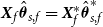 $\textbf{\textit{v}}_3$
and
 $\textbf{\textit{v}}_4$
. We show that
 $\textbf{\textit{v}}_1 = \textbf{\textit{v}}_2 = \textbf{\textit{v}}_3 = \textbf{\textit{v}}_4 = \textbf{0}$
; this will establish invariance of fitted and forecast values.
It is convenient to use a double-suffix notation to identify the entries in  $\textbf{\textit{v}}_1$
,
 $\textbf{\textit{v}}_2$
,
 $\textbf{\textit{v}}_3$
and
 $\textbf{\textit{v}}_4$
. Thus, cell (i, j) is associated with
 $\textbf{\textit{v}}_1(i, j)$
and corresponds to the
 $n_a(j-1) + i$
entry in
 $\textbf{\textit{v}}_1$
; we have a similar correspondence for
 $\textbf{\textit{v}}_2$
,
 $\textbf{\textit{v}}_3$
and
 $\textbf{\textit{v}}_4$
. We check invariance region by region.
Consider region 1. Suppose cell (i, j) lies in region 1 with cohort index  $n_a - i + j$
. We pick out the terms in A, B, C and D from (54), (55), (56) and (57) as appropriate. The bracket notation
 $(\;)$
indicates which terms in
 $\textbf{\textit{X}}^*_f (\hat {\boldsymbol{\theta}}^*_{s, f} - \hat {\boldsymbol{\theta}}^*_{r, f})$
are used, i.e.,
 $\boldsymbol{\alpha}$
,
 $\boldsymbol{\kappa}$
,
 $\boldsymbol{\gamma}$
and
 $\boldsymbol{\beta}$
in turn,
 \begin{eqnarray*} A &:& (1) + (-1) + (0) + (0) = 0 \\[4pt] B &:& (1) + (0) + (-1) + (0) = 0 \\[4pt] C &:& (i + \omega_a) + (-j) + (n_a - i + j - \omega_c) + (0) = 0 \\[4pt] D &:& (0) + (j - \bar y) + (0) + (\bar y - j) = 0\end{eqnarray*}
and we have verified invariance in region 1. Of course, we already knew this from the general result on fitted values.
In region 2, we consider the j-ahead forecast for  $\boldsymbol{\kappa}$
. This is cell
 $(i, n_y + j)$
with cohort index
 $n_a - i + n_y + j$
. Using (54), (56), (57) and (58), we find
 \begin{eqnarray*} A &:& (1) + (-1) + (0) + (0) = 0 \\[4pt] B &:& (1) + (0) + (-1) + (0) = 0 \\[4pt] C &:& (i + \omega_a) + (- n_ y - j) + (n_a - i + n_y + j - \omega_c) + (0) = 0 \\[4pt] D &:& (0) + (n_y - \bar y + j) + (0) + (\bar y - n_y - j) = 0\end{eqnarray*}
as required. Finally, in region 3, we consider the j-ahead forecast for  $\boldsymbol{\gamma}$
. For age i, we have the
 $(i+j-1)$
-ahead forecast for
 $\boldsymbol{\kappa}$
, i.e., cell
 $(i, n_y + i + j -1)$
. We use (54), (57), (58) and (59) and find
 \begin{eqnarray*} A &:& (1) + (-1) + (0) + (0) = 0 \\[4pt] B &:& (1) + (0) + (-1) + (0) = 0 \\[4pt] C &:& (i + \omega_a) + (- n_ y - i - j + 1) + (n_c - \omega_c + j) + (0) = 0 \\[4pt] D &:& (0) + (n_y - \bar y + i + j - 1) + (0) + (\bar y - n_y - i - j + 1) = 0\end{eqnarray*}
We conclude that the fitted and forecast values are invariant with respect to the choice of constraints when an ARIMA $(p, \delta, q)$
model with fitted mean,
 $\delta =1$
or 2, is used to forecast. We note that the proof of invariance in the smooth APC model is a special case of the above. In (52), we omit the final row and column, and we have reduced (52) to (42).
4.4 Lee–Carter model
The Lee–Carter model or LC model (Lee & Carter, Reference Lee and Carter1992) is the benchmark model for modelling and forecasting mortality. The LC model is a non-linear model so the methods of the previous sections do not apply. However, we can still use our extended algorithm (15) to fit two forms of the model: Lee and Carter’s original formulation and a smooth version.
4.4.1 LC model
The LC model is
 \begin{equation} \log \mu_{x, y} = \alpha_x + \beta_x \kappa_y,\, x = 1,\ldots, n_a,\, y = 1,\ldots, n_y\end{equation}
We require one location and one scale constraint to make the parameters estimable. We use
 \begin{equation} \sum \kappa_y = 0,\; \sum \beta_x = 1\end{equation}
as in Lee & Carter (Reference Lee and Carter1992). The following transformation leaves the fitted values of  $\log \boldsymbol{\mu}$
unchanged for any values of A and B.
 \begin{equation} \alpha_x + \beta_x \kappa_y \mapsto (\alpha_x + A\beta_x) + (\beta_x/B)(B \kappa_y - AB) = \alpha_x^* + \beta_x^* \kappa_y^*\end{equation}
Let  $\hat {\boldsymbol{\alpha}}_s$
,
 $\hat {\boldsymbol{\beta}}_s$
and
 $\hat {\boldsymbol{\kappa}}_s$
be the maximum likelihood estimates of
 $\boldsymbol{\alpha}_s$
,
 $\boldsymbol{\beta}_s$
and
 $\boldsymbol{\kappa}_s$
under the constraints (61) with the usual corresponding notation for the estimates
 $\hat {\boldsymbol{\alpha}}_r$
,
 $\hat {\boldsymbol{\beta}}_r$
and
 $\hat {\boldsymbol{\kappa}}_r$
under some random constraint system. It follows from (62) that
 \begin{eqnarray} \hspace*{-16pt}\hat {\boldsymbol{\alpha}}_s &=& \hat {\boldsymbol{\alpha}}_r + A \hat {\boldsymbol{\beta}}_r \end{eqnarray}
 \begin{eqnarray} \hspace*{-33pt}\hat {\boldsymbol{\beta}}_s &=& \hat {\boldsymbol{\beta}}_r/B \end{eqnarray}
 \begin{eqnarray} \hat {\boldsymbol{\kappa}}_s &=& B \hat {\boldsymbol{\kappa}}_r - AB \textbf{1}_{n_y}\end{eqnarray}
for some scalars A and B.
Brouhns et al. (Reference Brouhns, Denuit and Vermunt2002) used maximum likelihood to estimate the parameters. We also use maximum likelihood but use (15); this is a full Newton–Raphson scheme which allows estimation with both smoothing and constraints. Following Currie (Reference Currie2013), we consider two coupled GLMs:
 \begin{align} \mbox{GLM1:}\, \log \boldsymbol{\mu} = \textbf{1}_{n_y} \otimes \tilde {\boldsymbol{\alpha}} + \textbf{\textit{X}}_1 \boldsymbol{\beta},\; \textbf{\textit{X}}_1 = \tilde {\boldsymbol{\kappa}} \otimes \textbf{\textit{I}}_{n_a} \end{align}
 \begin{align} \hspace{6.5pt}\mbox{GLM2:}\,\log \boldsymbol{\mu} = \textbf{\textit{X}}_2 \boldsymbol{\theta} , \; \textbf{\textit{X}}_2 = [\textbf{1}_{n_y} \otimes \textbf{\textit{I}}_{n_a} \, :\ \textbf{\textit{I}}_{n_y} \otimes \tilde {\boldsymbol{\beta}}]\end{align}
where  $\boldsymbol{\theta} = (\boldsymbol{\alpha}^\prime, \boldsymbol{\kappa}^\prime)^\prime$
; here
 $\tilde{\boldsymbol{\alpha}}$
,
 $\tilde {\boldsymbol{\beta}}$
and
 $\tilde{\boldsymbol{\kappa}}$
represent current estimates of
 $\boldsymbol{\alpha}$
,
 $\boldsymbol{\beta}$
and
 $\boldsymbol{\kappa}$
, respectively. Both GLM1 and GLM2 are in the class defined in equation (1) but note that in GLM1 the offset is
 $\log \textbf{\textit{e}} + \textbf{1}_{n_y} \otimes \tilde {\boldsymbol{\alpha}}$
. In GLM1, we estimate
 $\boldsymbol{\beta}$
for current values of
 $\boldsymbol{\alpha}$
and
 $\boldsymbol{\kappa}$
, while in GLM2 we estimate
 $\boldsymbol{\alpha}$
and
 $\boldsymbol{\kappa}$
for given values of
 $\boldsymbol{\beta}$
. We now iterate between GLM1 and GLM2 until convergence.
We fit the model with (a) the standard constraints (61) and (b) the random constraints in GLM1 on  $\boldsymbol{\beta}$
, i.e.,
 $\sum_1^{n_a} u_i \beta_i = 1$
, and the random constraints in GLM2 on
 $\boldsymbol{\theta} = (\boldsymbol{\alpha}^\prime, \boldsymbol{\kappa})^\prime$
, i.e.,
 $\sum_1^{n_a+n_y} u_i\theta_i = 0$
; the
 $u_i$
are independent
 $\mathcal{U}(0,\,1)$
.
The upper panels and the lower left panel of Figure 8 show the estimates of  $\boldsymbol{\alpha}$
,
 $\boldsymbol{\kappa}$
and
 $\boldsymbol{\beta}$
, respectively, under the standard and random constraints. In our example, we found
 $A = 5.907$
,
 $B = 1.983$
and
 $AB = 11.71$
. The parameter estimates in Figure 8 satisfy (63), (64) and (65) with these values of A and B. The lower right panel shows the single (invariant) estimate of log mortality at age 65.
Parameter estimates in the LC model (60) under standard and random constraints:  $\hat {\boldsymbol{\alpha}}_s = \hat {\boldsymbol{\alpha}}_r + A \hat {\boldsymbol{\beta}}_r$
,
 $\hat {\boldsymbol{\beta}}_s = \hat {\boldsymbol{\beta}}_r/B$
,
 $\hat {\boldsymbol{\kappa}}_s = B \hat {\boldsymbol{\kappa}}_r - AB \textbf{1}_{n_y}$
;
 $A = 5.907$
,
 $B= 1.983$
and
 $AB = 11.71$
. Fitted invariant
 $\log \mu$
for age 65.

Forecasting in the LC model is particularly straightforward. As usual, we forecast with an ARIMA(p,  $\delta$
, q) model,
 $\delta=1$
or 2. Let
 $\hat {\boldsymbol{\kappa}}_{s, f}$
and
 $\hat {\boldsymbol{\kappa}}_{r, f}$
denote some forecast values of
 $\hat {\boldsymbol{\kappa}}_s$
and
 $\hat {\boldsymbol{\kappa}}_r$
, respectively. We have from (65)
 $\hat{\boldsymbol{\kappa}}_s = B\hat {\boldsymbol{\kappa}}_r - AB \textbf{1}_{n_y}$
; it follows immediately from Appendix C that
 $\hat {\boldsymbol{\kappa}}_{s, f} = B\hat {\boldsymbol{\kappa}}_{r, f} - AB \textbf{1}_{n_f}$
, where
 $n_f$
is the number of years in the forecast. Thus, the forecasts of
 $\boldsymbol{\kappa}$
satisfy (65), and hence forecasts of mortality are invariant with respect to the choice of constraint system.
4.4.2 Smooth LC model
One unsatisfactory feature of the Lee–Carter model, particularly for actuaries, is that irregularities in the estimate of  $\boldsymbol{\beta}$
lead to irregular forecasts of mortality at individual ages and can even lead to forecasts at adjacent ages crossing over; see Currie (Reference Currie2013) for examples of this behaviour. Delwarde et al. (Reference Delwarde, Denuit and Eilers2007) addressed this problem by smoothing the estimate of
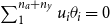 $\boldsymbol{\beta}$
with the method of P-splines. They set
 $\boldsymbol{\beta} = \textbf{\textit{B}}_a \textbf{\textit{b}}$
, where
 $\textbf{\textit{B}}_a$
is a regression matrix evaluated on a basis of B-splines along age. The model matrix for GLM1 in (66) becomes
 \begin{equation*} \mbox{GLM1:} \quad \log \boldsymbol{\mu} = \textbf{1}_{n_y} \otimes \tilde {\boldsymbol{\alpha}} + \textbf{\textit{X}}_1 \textbf{\textit{b}},\; \textbf{\textit{X}}_1 = \tilde {\boldsymbol{\kappa}} \otimes \textbf{\textit{B}}_a\end{equation*}
However,  $[\tilde {\boldsymbol{\kappa}} \otimes \textbf{\textit{B}}_a] \textbf{\textit{b}} = [\tilde {\boldsymbol{\kappa}} \otimes \textbf{\textit{I}}_{n_a}] \boldsymbol{\beta}$
, i.e., we are back in the model definition (66). The model matrix for GLM2 is not affected by the smoothing of
 $\boldsymbol{\beta}$
. We deduce that (63), (64) and (65) hold in the smooth case too. We conclude that invariance of fitted and forecast values holds for the smooth model. Numerical work supports this conclusion.
4.5 Other models
We have described our method by giving a detailed discussion of a number of examples. The method can be applied to other mortality models and we mention two briefly.
4.5.1 CBD model with cohort effects
Cairns et al. (Reference Cairns, Blake and Dowd2006) introduced the model  $\log \mu_{x, y} =\kappa_y^{(1)} + (x-\bar x)\kappa_y^{(2)}$
which is often referred to as the CBD model. Cairns et al. (Reference Cairns, Blake, Dowd, Coughlan, Epstein, Ong and Balevich2009) modified this model with the addition of cohort effects:
 \begin{equation} \log \mu_{x, y} = \kappa_y^{(1)} + \kappa_y^{(2)}(x-\bar x) + \gamma_{c(x, y)},\; x = 1,\ldots, n_a,\, y =1,\ldots,n_y\end{equation}
where  $\bar x$
is the mean age. The model matrix is
 \begin{equation} \textbf{\textit{X}} = [\textbf{\textit{I}}_{n_y} \otimes \textbf{1}_{n_a}\ :\ \textbf{\textit{I}}_{n_y} \otimes (\textbf{\textit{x}}_a - \bar x \textbf{1}_{n_a})\ :\ \textbf{\textit{X}}_c].\end{equation}
The coefficient vector is  $\boldsymbol{\theta} = ({\boldsymbol{\kappa}^{(1)}}^\prime,{\boldsymbol{\kappa}^{(2)}}^\prime, \boldsymbol{\gamma}^\prime)^\prime$
with length
 $n_a+ 3n_y - 1$
. The rank of
 $\textbf{\textit{X}}$
is
 $n_a + 3n_y - 3$
, so two constraints are required to give unique parameter estimates. We use
 $\sum \gamma_c = \sum c \gamma_c = 0$
as our standard constraints (Cairns et al., Reference Cairns, Blake, Dowd, Coughlan, Epstein, Ong and Balevich2009) and two sets of random constraints on
 $\boldsymbol{\theta}$
. We compute
 $\mathcal{N}(\textbf{\textit{X}})$
, the null space of
 $\textbf{\textit{X}}$
, and conclude that
 \begin{eqnarray} \boldsymbol{\kappa}^{(1)}_r &=& \boldsymbol{\kappa}^{(1)}_s + [A + (\bar x - n_x)B] \textbf{1}_{n_y} - B \textbf{\textit{x}}_y \nonumber \\ \boldsymbol{\kappa}^{(2)}_r &=& \boldsymbol{\kappa}^{(2)}_s + B \textbf{1}_{n_y} \end{eqnarray}
 \begin{align} \hspace*{-65pt}\boldsymbol{\gamma}_r = \boldsymbol{\gamma}_s - A \textbf{1}_c + B \textbf{\textit{x}}_c \nonumber\end{align}
where we have used our usual notation for the estimates under the standard and random constraints. Once again we see that the parameters are linearly related, so provided we choose a forecasting method which preserves these relationships we can conclude that the forecasts of mortality are invariant with respect to the choice of constraints.
4.5.2 Reduced Plat model
Plat (Reference Plat2009) proposed the model
 \begin{equation} \log \mu_{x, y} = \alpha_x + \kappa_y^{(1)} + (x-\bar x)\kappa_y^{(2)} + \gamma_{c(x, y)},\; x = 1,\ldots, n_a,\, y =1,\ldots,n_y\end{equation}
Hunt & Blake (Reference Hunt and Blake2020b) refer to this model as the reduced Plat model. We see that it is formally equivalent to the unsmoothed APCI model (44) so the dimension of its null space,  $\mathcal{N}(\textbf{\textit{X}})$
, is five, as is readily verified directly. In particular,
 $\mathcal{N}(\textbf{\textit{X}})$
has a quadratic term, as in (46). This means that an ARIMA(p,1,q) model will not lead to invariant forecasts. We can smooth the age term with a second-order penalty; this will reduce the dimension of the null space from five to four, just as in APCI model, removing the quadratic term from
 $\mathcal{N}(\textbf{\textit{X}})$
. Once more, we are back in the linear case. We will comment further on this increase in the effective rank of the model in our concluding remarks.
5 Conclusions
There are three new ideas in this paper.
(a) The standard approach to modelling and forecasting of mortality specifies a particular set of constraints that enables parameters to be estimated uniquely; often there are arguments to support this choice. Our approach is to consider the difference in the parameter estimates obtained with two different constraint systems. These differences are characterised by the null space of the model matrix. This approach enabled us to deduce that, while parameters are not identifiable, (i) fitted values of mortality are identifiable (a known result) and (ii) forecast values of mortality too are identifiable for ARIMA(p,
 $\delta$
, q) models with a fitted mean where
$\delta = 1$
or 2.
(b) Our second contribution is the idea of the effective rank of a model. We could describe a constraint like
$\sum \kappa_y = 0$
in the AP model, the APC model or the APCI model as an explicit or hard constraint. The P-spline system constrains the regression coefficients by forcing a certain level of smoothness on them; we could call this an implicit or soft constraint. We saw in our discussion of the APC model and particularly of the APCI model that in some cases this soft constraint can increase the effective rank of the model, i.e., smoothing can act like a hard constraint.(c) Our third idea is the use of random constraints. In this paper, we have used random constraints to illustrate our theoretical discussion. Random constraints also have an important practical use since their use avoids the need to calculate a null space for the model. The fitting algorithm (15) makes it straightforward to fit with any constraint system. A practical method of checking whether forecasting is invariant with respect to the choice of constraints is to forecast with both a given and a random constraint system. If the forecasts are equal it is reasonable to assume that forecasting is invariant with respect to the choice of constraints.


The results in this paper are given for the principal case of interest to actuaries, namely, when we have a GLM for the force of mortality,  $\mu_{x, y}$
, and deaths are distributed according to the Poisson distribution. However, the results depend only on the assumption of a GLM and the structure of the model matrix
 $\textbf{\textit{X}}$
. The actuary may choose to model
 $q_{x, y}$
, the probability of death at age x in year y. We assume a binomial distribution,
 $D_{x, y} \sim \mathcal{B}(E_{x, y}, q_{x, y})$
, where
 $E_{x, y}$
is the initial exposed to risk. The results on the invariance of fitted and forecast values of
 $q_{x, y}$
all go through without alteration. One could even make the simpler assumption that
 $\log(D_{x, y}/e_{x, y}) \sim \mathcal{N}(\log\,\mu_{x, y}, \sigma^2)$
; our results apply here too.
The CMI gave a particular set of transformations of the parameters in the APCI model which left the values of  $\log \boldsymbol{\mu}$
unchanged (CMI, 2016a, 7.3). We saw in our discussion of this model that this set of transformations corresponded to a particular basis for the null space of the model matrix. This is a good approach if a suitable set of transformations can be found. When smoothing is applied, it does not seem obvious that such a set of transformations can easily be found. In this case, we have provided a systematic method for computing a basis for the null space.
In Appendix B, we gave a simple method for fitting a generalised linear model with specified constraints which exploited the invariance of fitted values to the choice of constraints. The result is given when the parameters are not subject to smoothing. It is possible to extend this approach when there is smoothing of some model terms and we will return to this topic in future work.
This paper has focussed on invariance. This is an attractive mathematical property, but the actuary may have reasons for choosing a forecasting model which does not lead to invariant forecasts; this is particularly true for the forecasting of the cohort parameters. In the APC model, for example, estimates of the cohort parameters under different constraint systems differ by a linear function. We have argued that the choice of forecasting method should preserve this relationship. This places a restriction on the class of forecasting models available, namely to ARIMA models with a fitted mean. The actuary should be aware that a choice outside this class may not lead to invariant forecasts.
Our discussion of effective rank in (b) above raises an interesting and not easily resolved question. Smoothing the age parameters  $\boldsymbol{\alpha}$
and
 $\boldsymbol{\beta}$
with a second-order penalty in the APCI model (and the age parameters
 $\boldsymbol{\alpha}$
in the reduced Plat model) leads to a reduction in the number of constraints required to produce unique estimates of the parameters from five in the unsmoothed model to four. If a third-order penalty is used, the number of constraints required is again five. Some readers may worry that the number of constraints should depend on the details of the smoothing method adopted. Certainly, smoothing in the APCI and reduced Plat model can have a large effect on parameter estimates, a consequence of the change in the effective rank of the model. In contrast, smoothing has very little effect on the invariant quantities, the fitted and forecast values of mortality.
The R language has its own way of dealing with models which are not of full rank: it deletes columns of the  $\textbf{\textit{X}}$
matrix until the remaining columns give a model matrix which is of full rank. For example, in the APC model, the columns corresponding to the most recent year and the two youngest cohorts are deleted; in the list of the estimated coefficients, these three parameters are reported as NA, i.e., not available. Explicit constraints are not used, and R’s reporting emphasises the non-identifiability of the parameters without further assumption. A particular set of constraints corresponds to such an assumption; this is a strong assumption and one not easily verified. Of course, there are implicit constraints here and the reported parameters correspond to the explicit constraints
 $\kappa_{n_y} = \gamma_{n_c-1} = \gamma_{n_c} = 0$
.
The practising actuary uses many mortality models in their daily work. Nearly all of these models require identifiability constraints. Our results tell us that we can be relaxed about the choice of constraint system. Forecast values will not depend on this choice provided we stay within the class of models used in this paper. This is a most reassuring conclusion.
Acknowledgements
I am grateful to Torsten Kleinow for suggesting this problem, to Stephen Richards for many helpful comments on earlier versions of this paper, and to Jim Howie for a most helpful tutorial on matrices and their null spaces. I am also grateful to the anonymous referee for a most helpful and thorough report which led to many clarifications and improvements to the presentation.
A Appendix
A.1 Some matrix results on invariance
We consider a model with model matrix  $\textbf{\textit{X}}$
and regression coefficients
 $\boldsymbol{\theta}$
. The number of constraints on
 $\boldsymbol{\theta}$
required to give a unique estimate of
 $\boldsymbol{\theta}$
is determined by the rank of
 $\textbf{\textit{X}}$
which we denote by
 $r(\textbf{\textit{X}})$
. The definition of
 $r(\textbf{\textit{X}})$
depends on a fundamental result in matrix theory. We need two definitions: the row rank of
 $\textbf{\textit{X}}$
is the maximum number of linearly independent rows of
 $\textbf{\textit{X}}$
; similarly, the column rank of
 $\textbf{\textit{X}}$
is the maximum number of linearly independent columns of
 $\textbf{\textit{X}}$
. Then, it can be proved that the row rank of
 $\textbf{\textit{X}}$
equals its column rank; this common value is known as the rank of
 $\textbf{\textit{X}}$
. For a proof of this result see, for example, Searle (Reference Searle1982, chapter 6).
The relationship between different estimates of  $\boldsymbol{\theta}$
under different constraint systems is determined by the null space of
 $\textbf{\textit{X}}$
. We denote the null space of
 $\textbf{\textit{X}}$
by
 $\mathcal{N}(\textbf{\textit{X}})$
and define
 \begin{equation*} \mathcal{N}(\textbf{\textit{X}}) = \{\textbf{\textit{v}}\,{:}\,\textbf{\textit{X}} \textbf{\textit{v}} = \textbf{0}\}\end{equation*}
For our purposes, the following result is fundamental.
Proposition A.1. For any matrix  $\textbf{\textit{X}}$
 \begin{equation} \mathcal{N}(\textbf{\textit{X}}^\prime \textbf{\textit{X}}) = \mathcal{N}(\textbf{\textit{X}})\end{equation}
Proof. First, let  $\textbf{\textit{v}} \in \mathcal{N}(\textbf{\textit{X}}^\prime\textbf{\textit{X}})$
. Then
 \begin{align*} \textbf{\textit{X}}^\prime \textbf{\textit{X}} \textbf{\textit{v}} = \textbf{0} \Rightarrow \textbf{\textit{v}}^\prime \textbf{\textit{X}}^\prime \textbf{\textit{X}} \textbf{\textit{v}} = 0 \Rightarrow (\textbf{\textit{X}} \textbf{\textit{v}})^\prime (\textbf{\textit{X}} \textbf{\textit{v}}) = 0 \Rightarrow \textbf{\textit{X}} \textbf{\textit{v}} = \textbf{0} \Rightarrow \textbf{\textit{v}} \in \mathcal{N}(\textbf{\textit{X}})\end{align*}
Conversely, let  $\textbf{\textit{v}} \in \mathcal{N}(\textbf{\textit{X}}),$
then
 $\textbf{\textit{X}} \textbf{\textit{v}} = \textbf{0}\Rightarrow \textbf{\textit{X}}^\prime \textbf{\textit{X}} \textbf{\textit{v}} = \textbf{0} \Rightarrow \textbf{\textit{v}} \in \mathcal{N}(\textbf{\textit{X}}^\prime \textbf{\textit{X}})$
.
Hence,  $\mathcal{N}(\textbf{\textit{X}}^\prime \textbf{\textit{X}}) = \mathcal{N}(\textbf{\textit{X}})$
.□
We wish to show that the fitted values in a GLM are invariant with respect to the choice of constraints. We consider first the standard linear regression model with normal errors and common variance; the result for a GLM will follow.
Proposition A.2. Define the regression model
 \begin{equation}\textbf{\textit{y}} = \textbf{\textit{X}} \boldsymbol{\theta} + \boldsymbol{\epsilon}, \; \textbf{\textit{X}},\, n \times p, n > p, r(\textbf{\textit{X}}) = p - q, q \ge 1\end{equation}
Let  $\hat {\boldsymbol{\theta}}_1$
and
 $\hat {\boldsymbol{\theta}}_2$
be any two solutions of the normal equations
 \begin{equation} \textbf{\textit{X}}^\prime \textbf{\textit{X}} \hat {\boldsymbol{\theta}} = \textbf{\textit{X}}^\prime \textbf{\textit{y}}\end{equation}
Then,
 \begin{equation} \textbf{\textit{X}} \hat {\boldsymbol{\theta}}_1 = \textbf{\textit{X}} \hat {\boldsymbol{\theta}}_2\end{equation}
Proof: Since  $\hat {\boldsymbol{\theta}}_1$
and
 $\hat {\boldsymbol{\theta}}_2$
satisfy the normal equations (A.3)
 \begin{eqnarray*} &\textbf{\textit{X}}^\prime \textbf{\textit{X}} (\hat {\boldsymbol{\theta}}_1 - \hat {\boldsymbol{\theta}}_2) = \textbf{\textit{X}}^\prime \textbf{\textit{y}} - \textbf{\textit{X}}^\prime \textbf{\textit{y}} = \textbf{0} \\
\Rightarrow & \hat {\boldsymbol{\theta}}_1 - \hat {\boldsymbol{\theta}}_2 \in \mathcal{N}(\textbf{\textit{X}}^\prime \textbf{\textit{X}}) = \mathcal{N}(\textbf{\textit{X}}) \quad \mbox{by (\linkref{dispA1}{A.1})} \\
\Rightarrow & \textbf{\textit{X}} \hat {\boldsymbol{\theta}}_1 = \textbf{\textit{X}} \hat {\boldsymbol{\theta}}_2\end{eqnarray*}
as required. □
A square matrix  $\textbf{\textit{A}}$
is positive semi-definite if
 $\textbf{\textit{v}}^\prime \textbf{\textit{A}} \textbf{\textit{v}} \ge 0$
for all
 $\textbf{\textit{v}}$
. We first prove:
Proposition A.3. Let  $\textbf{\textit{A}}$
be a symmetric, positive semi-definite matrix. If
 $\textbf{\textit{v}}^\prime \textbf{\textit{A}} \textbf{\textit{v}} = 0$
, then
 $\textbf{\textit{v}} \in \mathcal{N}(\textbf{\textit{A}})$
.
Proof. Since  $\textbf{\textit{A}}$
is a symmetric, positive semi-definite matrix, there exists a matrix
 $\textbf{\textit{K}}$
such that
 $\textbf{\textit{A}} = \textbf{\textit{K}}^\prime\textbf{\textit{K}}$
; see Searle (Reference Searle1982, chapter 7) for example. Hence,
 \begin{equation*} \textbf{\textit{v}}^\prime \textbf{\textit{A}} \textbf{\textit{v}} = 0 \Rightarrow \textbf{\textit{v}}^\prime \textbf{\textit{K}}^\prime \textbf{\textit{K}} \textbf{\textit{v}} = 0 \Rightarrow (\textbf{\textit{K}} \textbf{\textit{v}})^\prime (\textbf{\textit{K}} \textbf{\textit{v}}) = 0 \Rightarrow \textbf{\textit{K}} \textbf{\textit{v}} = \textbf{0} \Rightarrow \textbf{\textit{K}}^\prime \textbf{\textit{K}} \textbf{\textit{v}} = \textbf{0}\end{equation*}
and  $\textbf{\textit{v}} \in \mathcal{N}(\textbf{\textit{A}})$
. □
We need a definition: the dimension of the null space of a matrix  $\textbf{\textit{X}}$
is the number of vectors in its basis; we denote this by
 $\mbox{dim}[\mathcal{N}(\textbf{\textit{X}})]$
. In general, we have
Proposition A.4. Let  $\textbf{\textit{A}}$
and
 $\textbf{\textit{B}}$
be symmetric, positive semi-definite matrices of the same size. Then
(a)
$\mathcal{N}(\textbf{\textit{A}} + \textbf{\textit{B}}) = \mathcal{N}(\textbf{\textit{A}}) \cap \mathcal{N}(\textbf{\textit{B}})$
, and(b)
$r(\textbf{\textit{A}} + \textbf{\textit{B}}) \ge \mbox{max}\{r(\textbf{\textit{A}}), r(\textbf{\textit{B}})\}$
.


Proof. Let  $\textbf{\textit{v}} \in \mathcal{N}(\textbf{\textit{A}} + \textbf{\textit{B}})$
. Then
 $(\textbf{\textit{A}} +\textbf{\textit{B}})\textbf{\textit{v}} = \textbf{0} \Rightarrow \textbf{\textit{v}}^\prime (\textbf{\textit{A}} + \textbf{\textit{B}})\textbf{\textit{v}} = 0\Rightarrow \textbf{\textit{v}}^\prime \textbf{\textit{A}} \textbf{\textit{v}} + \textbf{\textit{v}}^\prime \textbf{\textit{B}}\textbf{\textit{v}} = 0\Rightarrow \textbf{\textit{v}}^\prime \textbf{\textit{A}} \textbf{\textit{v}} = 0$
and
 $\textbf{\textit{v}}^\prime \textbf{\textit{B}} \textbf{\textit{v}} = 0$
since both
 $\textbf{\textit{A}}$
and
 $\textbf{\textit{B}}$
are positive semi-definite. Hence, by Proposition A.3,
 $\textbf{\textit{v}} \in \mathcal{N}(\textbf{\textit{A}})$
and
 $\textbf{\textit{v}} \in \mathcal{N}(\textbf{\textit{B}}) \Rightarrow \textbf{\textit{v}} \in\mathcal{N}(\textbf{\textit{A}})\cap\, \mathcal{N}(\textbf{\textit{B}})$
.
Clearly, if  $\textbf{\textit{v}} \in \mathcal{N}(\textbf{\textit{A}}) \cap \mathcal{N}(\textbf{\textit{B}}),$
then
 $\textbf{\textit{v}} \in \mathcal{N}(\textbf{\textit{A}} + \textbf{\textit{B}})$
and (a) is proved.
Furthermore, it follows from (a) that
 \begin{equation*} \mbox{dim}[\mathcal{N}(\textbf{\textit{A}} + \textbf{\textit{B}})] \le \mbox{min}\{\mbox{dim}[\mathcal{N}(\textbf{\textit{A}})], \mbox{dim}[\mathcal{N}(\textbf{\textit{B}})]\}\end{equation*}
and (b) follows immediately from the rank-nullity theorem; see Searle, (Reference Searle1982, chapter 6) for example.□
In our case, we take  $\textbf{\textit{A}} = \textbf{\textit{X}}^\prime \textbf{\textit{X}}$
and
 $\textbf{\textit{B}} = \textbf{\textit{P}}$
, where
 $\textbf{\textit{P}}$
is a penalty matrix. The result tells us that smoothing may reduce the number of constraints required to obtain a unique estimate of
 $\boldsymbol{\theta}$
.
An immediate corollary of Proposition A.4 is the invariance result for fitted values in a penalised regression.
Corollary: Let  $\hat {\boldsymbol{\theta}}_1$
and
 $\hat {\boldsymbol{\theta}}_2$
be any two solutions of the penalised normal equations
 \begin{equation*} (\textbf{\textit{X}}^\prime \textbf{\textit{X}} + \textbf{\textit{P}}) \hat {\boldsymbol{\theta}} = \textbf{\textit{X}}^\prime \textbf{\textit{y}}\end{equation*}
Then
 \begin{equation*} \textbf{\textit{X}} \hat {\boldsymbol{\theta}}_1 = \textbf{\textit{X}} \hat {\boldsymbol{\theta}}_2\end{equation*}
Proof. By assumption, we have
 \begin{eqnarray*} \hat {\boldsymbol{\theta}}_1 - \hat {\boldsymbol{\theta}}_2 &\in& \mathcal{N}(\textbf{\textit{X}}^\prime \textbf{\textit{X}} + \textbf{\textit{P}}) \\
&=& \mathcal{N}(\textbf{\textit{X}}^\prime \textbf{\textit{X}}) \cap \mathcal{N}(\textbf{\textit{P}})\; \mbox{by Proposition}\ \linkref{pro4}{{\rm A}.4} \\
&\subseteq & \mathcal{N}(\textbf{\textit{X}}^\prime \textbf{\textit{X}}) \\
&=& \mathcal{N}(\textbf{\textit{X}}) \; \mbox{by Proposition}\ \linkref{dispA1}{{\rm A}.1}\end{eqnarray*}
and  $\textbf{\textit{X}} \hat {\boldsymbol{\theta}}_1 = \textbf{\textit{X}} \hat {\boldsymbol{\theta}}_2$
as required. □
The extension of these results to a GLM is straightforward. The normal equations are replaced by the estimating equations (Nelder & Wedderburn, Reference Nelder and Wedderburn1972)
 \begin{equation} \textbf{\textit{X}}^\prime \textbf{\textit{W}} \textbf{\textit{X}} \hat {\boldsymbol{\theta}} = \textbf{\textit{X}}^\prime \textbf{\textit{W}} \textbf{\textit{z}}\end{equation}
where  $\textbf{\textit{W}}$
is the diagonal matrix of weights and
 $ \textbf{\textit{z}}$
is the working variable;
 $\hat {\boldsymbol{\theta}}$
is the updated estimate of
 $\boldsymbol{\theta}$
. Both
 $\textbf{\textit{W}}$
and
 $\textbf{\textit{z}}$
depend on the current estimated value of the mean. Suppose that
 $\textbf{\textit{W}}_0$
and
 $\textbf{\textit{z}}_0$
are the initial estimates of
 $\textbf{\textit{W}}$
and
 $\textbf{\textit{z}}$
which are computed from the initial estimate of the mean (usually the observed values y). Let
 $\hat {\boldsymbol{\theta}}_{0,1}$
and
 $\hat {\boldsymbol{\theta}}_{0,2}$
be any two initial solutions of (A.5). We write (A.5) as
 \begin{equation*} \textbf{\textit{X}}^{*\prime} \textbf{\textit{X}}^* \hat {\boldsymbol{\theta}} = \textbf{\textit{X}}^{*\prime} \textbf{\textit{z}}^*\end{equation*}
where  $\textbf{\textit{X}}^* = \textbf{\textit{W}}^{1/2} \textbf{\textit{X}}$
,
 $\textbf{\textit{z}}^* = \textbf{\textit{W}}^{1/2} \textbf{\textit{z}}$
and
 $\textbf{\textit{W}}^{1/2}$
is the diagonal matrix whose elements are the square roots of those of
 $\textbf{\textit{W}}$
. (We note that
 $\textbf{\textit{W}}^{1/2}$
exists since
 $\textbf{\textit{W}}$
is diagonal with positive diagonal entries.) Then by the invariance result (A.4), we have
 \begin{equation*} \textbf{\textit{X}}^* \hat {\boldsymbol{\theta}}_{0,1} = \textbf{\textit{X}}^* \hat {\boldsymbol{\theta}}_{0,2} \Rightarrow \textbf{\textit{X}} \hat {\boldsymbol{\theta}}_{0,1} = \textbf{\textit{X}} \hat {\boldsymbol{\theta}}_{0,2}\end{equation*}
Hence, the updated values of the mean are equal and so the updated values  $\textbf{\textit{W}}_1$
and
 $\textbf{\textit{z}}_1$
are also equal. Hence, as we iterate (A.5) until convergence, we have
 $\textbf{\textit{X}} \hat {\boldsymbol{\theta}}_{i,1} = \textbf{\textit{X}} \hat {\boldsymbol{\theta}}_{i,2}$
at the i th iteration. Hence, at convergence
 $\textbf{\textit{X}} \hat {\boldsymbol{\theta}}_1 = \textbf{\textit{X}}\hat {\boldsymbol{\theta}}_2$
where
 $\hat {\boldsymbol{\theta}}_1$
and
 $\hat {\boldsymbol{\theta}}_2$
are the converged values. Thus,
 $\hat {\boldsymbol{\theta}}_1 -\hat {\boldsymbol{\theta}}_2 \in \mathcal{N}(\textbf{\textit{X}})$
just as in the normal regression case. The extension to smoothing in a GLM follows as in the normal case.
B Appendix
B.1 Some R code on invariance
The fundamental invariance result (A.4) implies that we can compute a model fit subject to a particular set of constraints from any other fit of the same model under different constraints. Currie (Reference Currie2016, equation (31)) gives the following formula:
 \begin{equation} \hat {\boldsymbol{\theta}} = (\textbf{\textit{X}}^\prime \textbf{\textit{X}} + \textbf{\textit{H}}^\prime \textbf{\textit{H}})^{-1} \textbf{\textit{X}}^\prime \log \hat {\boldsymbol{\mu}}\end{equation}
Here,  $\textbf{\textit{X}}$
is the model matrix for, say, the APC model,
 $\log \hat{\boldsymbol{\mu}}$
is the (invariant) vector of fitted log mortalities and
 $\boldsymbol{\theta}$
is the parameter vector which is subject to the desired constraint
 $\textbf{\textit{H}} \boldsymbol{\theta} = \textbf{0}$
. In the case of the APC model,
 $\textbf{\textit{H}}$
is
 $3 \times (n_a+n_y+n_c)$
.
For example, let Dth, Exp, X and H be the R objects that contain the vectors of deaths and exposures, the model matrix and the constraints matrix, respectively. Then, the following computes  $\log \hat {\boldsymbol{\mu}}$
with R’s glm function and then computes
 $\hat {\boldsymbol{\theta}}$
subject to
 $\textbf{\textit{H}} \boldsymbol{\theta} = \textbf{0}$
from (B.1).
Fit.glm
<-glm(Dth $\sim$
X + offset(log(Exp)), family = poisson)
Log.Mu.hat <-log(Fit.glmfit/Exp)
Theta.hatsolve(t(X) %*% X + t(H) %*% H, t(X) %*% Log.Mu.hat)
We note in particular that we do not need to know what constraints the glm function has used to fit the model.
C Appendix
C.1 A time series result
We show that if two time series are linearly related and they are forecast with an ARIMA $(p,\,\delta,\,q)$
model with a fitted mean,
 $\delta= 1$
or 2, then the forecasts obey the same linear relationship. First, we prove a preliminary result. The proof uses discrete integration where the usual constant of integration corresponds to how the forecast is joined to the series to be forecast. The results correspond to how R computes a forecast.
Proposition A.5. Let  $\textbf{\textit{y}} = (y_1,\ldots,y_n)^\prime$
. There are two cases.
Case 1: $\delta = 1$
. Consider forecasting
 $\textbf{\textit{y}}$
with an ARIMA(p, 1, q) model. Let
 $\textbf{\textit{u}} = (u_1,\ldots,u_{n_f})^\prime$
be the forecast of length
 $n_f$
of first differences of
 $\textbf{\textit{y}}$
with an ARMA(p, q) model. Let
 $\textbf{\textit{y}}_f = (y_{n+1},\ldots,y_{n+n_f})^\prime$
be the forecast of length
 $n_f$
of
 $\textbf{\textit{y}}$
with the ARIMA(p, 1, q) model. Then
 \begin{equation} y_{n+j} = y_n +\sum_{k=1}^j u_k, \; j = 1,\ldots, n_f\end{equation}
Case 2: $\delta = 2$
. In a similar fashion, let
 $\textbf{\textit{v}} =(v_1,\ldots,v_{n_f})^\prime$
be the forecast of length
 $n_f$
of second differences of
 $\textbf{\textit{y}}$
with an ARMA(p, q) model. Now let
 $\textbf{\textit{y}}_f =(y_{n+1},\ldots,y_{n+n_f})^\prime$
be the forecast of length
 $n_f$
of
 $\textbf{\textit{y}}$
with the ARIMA(p, 2, q) model. Then
 \begin{equation} y_{n+j} = y_n +\sum_{k=1}^j w_k,\; j = 1,\ldots, n_f\end{equation}
where
 \begin{equation} w_k = y_n - y_{n-1} +\sum_{\ell=1}^k v_\ell,\; k = 1,\ldots, n_f\end{equation}
Proof. Case 1. Forecasting  $\textbf{\textit{y}}$
with an ARIMA(p, 1, q) is performed by fitting an ARMA(p, q) model to first differences of
 $\textbf{\textit{y}}$
and then reversing the differencing. With the above notation, we have
 \begin{align*} \nonumber y_{n+1} &= y_n + u_1 \\ y_{n+2} &= y_{n+1} + u_2 = y_n + u_1 + u_2, \; \mbox{and in general} \\ y_{n+j} &= y_{n+j-1} + u_j = y_n +\sum_{k=1}^j u_k\end{align*}
which is (C.1).
Case 2. Forecasting  $\textbf{\textit{y}}$
with an ARIMA(p, 2, q) is performed by fitting an ARMA(p, q) model to second differences of
 $\textbf{\textit{y}}$
and then reversing the differencing. Applying (C.1) once, we find
 \begin{equation*} y_{n+j} = y_n +\sum_{k=1}^j w_k\end{equation*}
where  $\textbf{\textit{w}} = (w_1,\ldots,w_{n_f})^\prime$
is the forecast of first differences of
 $\textbf{\textit{y}}$
. Applying (C.1) a second time to the series
 $\textbf{\textit{w}}$
yields
 \begin{equation*} w_k = y_n - y_{n-1} + \sum_{\ell=1}^k v_\ell\end{equation*}
as required. □
We can now prove
Proposition A.6. Let  $\textbf{\textit{y}} = (y_1,\ldots,y_n)^\prime$
and
 $\textbf{\textit{z}} = (z_1,\ldots,z_n)^\prime$
be two times series which are linearly related, i.e.,
 \begin{equation} \textbf{\textit{y}} = \textbf{\textit{z}} + a \textbf{{\em 1}} + b \textbf{\textit{x}} \end{equation}
for some a and b; here  $\textbf{\emph{1}}$
is the vector of 1s of length n and
 $\textbf{\textit{x}} = (1,\ldots,n)^\prime$
. Let
 $\textbf{\textit{y}}_f = (y_{n+1},\ldots, y_{n+n_f})^\prime$
and
 $\textbf{\textit{z}}_f= (z_{n+1},\ldots, z_{n+n_f})^\prime$
be the forecasts of
 $\textbf{\textit{y}}$
and
 $\textbf{\textit{z}}$
of length
 $n_f$
with an ARIMA
 $(p, \delta, q),\; \delta = 1,2$
model. Then,
 $\textbf{\textit{y}}_f$
and
 $\textbf{\textit{z}}_f$
obey the same linear relationship as
 $\textbf{\textit{y}}$
and
 $\textbf{\textit{z}}$
, i.e.,
 \begin{equation} \textbf{\textit{y}}_f = \textbf{\textit{z}}_f + a \textbf{\em 1} + b (n \textbf{\em 1} + \textbf{\textit{x}}_f) \end{equation}
where
$\textbf{\textit{x}}_f = (1,\ldots,n_f)^\prime$
.
Proof: Case 1:  $\delta = 1$
. We have from (C.4)
 \begin{equation} \Delta (\textbf{\textit{y}}) - b \textbf{1}_{n-1} = \Delta (\textbf{\textit{z}})\end{equation}
where  $\Delta$
indicates first-order differencing and
 $\textbf{1}_{n-1}$
is the vector of 1s of length
 $n-1$
. Let
 $\textbf{\textit{u}}$
and
 $\textbf{\textit{v}}$
be the forecasts, respectively, of
 $\Delta (\textbf{\textit{y}})$
and
 $\Delta (\textbf{\textit{z}})$
with an ARIMA(p, 0, q) model with a mean. Denote the fitted means by
 $\mu_u$
and
 $\mu_v$
. It follows immediately from (C.6) and the definition of an ARIMA model with a mean that
 $\mu_u = \mu_v +b$
. Hence
 \begin{equation} \textbf{\textit{u}} = \textbf{\textit{v}} + b \textbf{1}_{n-1}\end{equation}
We have
 \begin{align*} y_{n+j} - z_{n+j} &= y_n + \sum_{k=1}^j u_k - z_n - \sum_{k=1}^j v_k\;\; \mbox{by}\ (\linkref{pro1}{{\rm C}.1}) \\
&= y_n + \sum_{k=1}^j u_k - y_n + a +n b - \sum_{k=1}^j (u_k -b) \;\; \mbox{by}\ (\linkref{pro4}{{\rm C}.4})\ \mbox{and}\ (\linkref{pro7}{{\rm C}.7}) \\
&= a + (n + j) b\end{align*}
as required.
Case 2: $\delta = 2$
. We have
 \begin{equation} \Delta^2 (\textbf{\textit{y}}) - \Delta^2 (\textbf{\textit{z}}) = \textbf{0}_{n-2}\end{equation}
and so  $\textbf{\textit{u}} = \textbf{\textit{v}}$
where
 $\textbf{\textit{u}}$
and
 $\textbf{\textit{v}}$
are the forecasts of
 $\Delta^2 (\textbf{\textit{y}})$
and
 $\Delta^2 (\textbf{\textit{z}})$
with an ARIMA((p, 0, q) model, respectively. We apply (C.2) and (C.3). We have
 \begin{align*} y_{n+j} - z_{n+j} &= y_n + \sum_{k=1}^j \left(y_n - y_{n-1} + \sum_{\ell = 1}^k u_\ell \right) - z_n - \sum_{k=1}^j \left(z_n - z_{n-1} + \sum_{\ell = 1}^k v_\ell \right) \\ & = y_n + \sum_{k=1}^j (y_n - y_{n-1}) - y_n + a + n b - \sum_{k=1}^j (y_n - a - nb - y_{n-1} + a + (n -1)b) \\ & = \sum_{k=1}^j (y_n - y_{n-1}) + a + n b - \sum_{k=1}^j (y_n - y_{n-1} - b) \\ &= a + (n+j)b\end{align*}
as required. □