1 Introduction
The classical Blasius problem considers the steady unbounded flow of a homogeneous Newtonian fluid on either side of a fixed blade of negligible thickness at zero angle of attack. The fluid has non-zero viscosity, and the blade imposes a no-slip condition on the fluid. The flow sufficiently far from the blade is unaffected by the presence of the blade, and the effects of viscosity are confined to boundary layers on either side of the blade. Across these layers, the velocity adjusts from zero on the blade to the ‘slip velocity’ of the incident flow.
This problem was first studied by Prandtl over a century ago (Prandtl Reference Prandtl1905), and has historic significance by linking the theories of viscous and inviscid flows, which had been developed separately until then. Many generalisations and extensions of this basic problem have been studied since Prandtl’s original paper, and Schlichting & Gersten (Reference Schlichting and Gersten2003) provide a good overview. Important applications include aerofoils, where the angle of attack is non-zero or the blade is cambered and not straight, and the study of boundary layers on a bluff object such as a cylinder, predicting flow separation and giving a resolution to d’Alembert’s paradox (Acheson Reference Acheson1989).
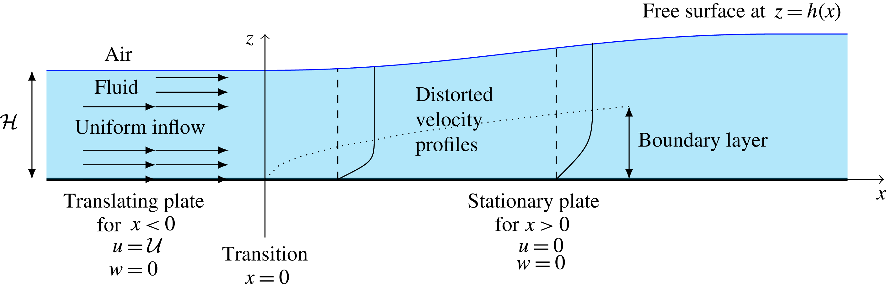
The moving plate problem to be studied in this article.

In this article, we consider the moving plate problem sketched in figure 1 and described below. A precise mathematical formulation will be given in § 2. A layer of a Newtonian liquid flows steadily over a rigid plane
 $z=0$
that consists of two plates. The plate upstream of a transition point
 $x=0$
translates with a speed
 $u={\mathcal{U}}$
. The downstream plate in
 $x>0$
is stationary. Both parts of the base impose a no-slip condition on the flow at
 $z=0$
. The air above the liquid is assumed to have negligible density and viscosity, and surface tension is ignored. Without loss of generality, the pressure at the free surface is taken to be zero. The flow is introduced far upstream with speed
 ${\mathcal{U}}$
and depth
 ${\mathcal{H}}$
.
In the limit of a layer of infinite depth
 ${\mathcal{H}}\rightarrow \infty$
, this problem becomes equivalent to the classical Blasius problem. With a finite depth for the upstream flow
 ${\mathcal{H}}<\infty$
, the effect of the no-slip condition in
 $x>0$
is initially confined to a boundary layer, as in the classical problem. The velocity profile in the boundary layer depends on the ‘outer flow’, i.e. the main body of the flow outside of the boundary layer. In particular, the boundary layer velocity profile must match with the ‘slip velocity’ that inviscid theory predicts for the outer flow, and is also governed by any pressure gradient in the outer flow. In the classical problem, the slip velocity is constant and there is no pressure gradient in the outer flow. With a free surface, the boundary layer has a stronger effect on the outer flow. The basal drag slows down the liquid in the boundary layer and causes a perpendicular displacement. This, in turn, affects the slip velocity and pressure gradient governing the boundary layer. Thus, the outer and boundary layers are coupled in the moving plate problem. This is in contrast to the classical problem, in which the coupling is only one way and the outer flow is externally imposed and may be taken to be completely uniform.
Our problem has two parameters that are not present in the classical problem, namely the finite upstream depth
 ${\mathcal{H}}$
and the gravitational acceleration
 $g$
. These can be encapsulated into two non-dimensional parameters: a Froude number
 $Fr={\mathcal{U}}/(g{\mathcal{H}})^{1/2}$
and a Reynolds number
 $Re={\mathcal{U}}{\mathcal{H}}/\unicode[STIX]{x1D708}$
based on the depth. Application of the classical theory to our present problem leads to the prediction that the Blasius boundary layer thickness should grow as
 $\unicode[STIX]{x1D6FF}(x)\sim (\unicode[STIX]{x1D708}x/{\mathcal{U}})^{-1/2}=Re^{-1/2}({\mathcal{H}}x)^{1/2}$
, where
 $\unicode[STIX]{x1D708}$
is the kinematic viscosity of the fluid. We shall show that this is also true of the boundary layer in this problem in the limit
 $Re\rightarrow \infty$
with
 $Fr>1$
fixed, but not for a certain distinguished limit in which
 $Re\rightarrow \infty$
and
 $Fr\rightarrow 1$
.
We assume throughout that the incident flow is supercritical, with
 $Fr>1$
; that is, the flow speed
 ${\mathcal{U}}$
is greater than the speed
 $(g{\mathcal{H}})^{1/2}$
of long surface waves (Chow Reference Chow1959; Billingham & King Reference Billingham and King2000). Supercriticality implies that no waves may travel arbitrarily far upstream: information about the presence of the transition at
 $x=0$
may not affect the upstream conditions as
 $x\rightarrow -\infty$
, although there is some effect in the upstream region
 $x<0$
. It is therefore possible to specify particular incident conditions as
 $x\rightarrow -\infty$
. Our analysis will not apply for subcritical flows
 $Fr<1$
, as then it is no longer appropriate to impose purely upstream conditions. We discuss the case
 $Fr<1$
in § 4.1.
We also assume that the flow is steady and laminar, but in practice the flow may be convectively unstable and may transition towards turbulence sufficiently far downstream. Boundary layer instability and transition to turbulence are also observed in the classical problem, and these processes are described in Schlichting & Gersten (Reference Schlichting and Gersten2003, §§ 3, 4). Similar problems have been studied in the context of channel flow, and experimental results on turbulent channel flows are outlined in Chow (Reference Chow1959, chap. 8). Nelson, Alving & Joseph (Reference Nelson, Alving and Joseph1995) considered the steady flow of a liquid driven by a shear stress due to a uniform wind blowing above the current, instead of driving by the bottom plate. Our problem has the advantage of being mathematically tractable, allowing analytical asymptotic expressions for the velocity profile. We shall outline possible applications of this work in § 4.4.
2 Mathematical statement of the problem
2.1 Notation
Let
 ${\mathcal{U}}$
and
 ${\mathcal{H}}$
respectively denote the incident speed and depth of the liquid. We take Cartesian coordinates
 $\boldsymbol{x}=(x,z)$
such that the base is positioned along
 $z=0$
, with the transition point at
 $x=0$
. The free surface is at
 $z=h(x)$
and the liquid occupies the region
 $0<z<h$
. The gravitational acceleration is
 $\boldsymbol{g}=(0,-g)$
, and let
 $\boldsymbol{u}=(u,w)$
denote the components of velocity. The incident flow velocity and depth are given by
 $\boldsymbol{u}\rightarrow ({\mathcal{U}},0)$
and
 $h\rightarrow {\mathcal{H}}>0$
as
 $x\ll -{\mathcal{H}}$
.
2.2 Non-dimensionalisation
We shall henceforth work in rescaled units such that
 ${\mathcal{U}}=1$
and
 ${\mathcal{H}}=1$
, and write everything in terms of the Reynolds and Froude numbers, instead of
 $g$
and
 $\unicode[STIX]{x1D708}$
. In these units, the flow rate
 $q={\mathcal{U}}{\mathcal{H}}=1$
. We also take the density of the liquid as
 $\unicode[STIX]{x1D70C}=1$
, and assume that the air above has negligible density.
2.3 Governing equations and boundary conditions
In terms of the non-dimensionalised quantities, the steady Navier–Stokes equations read as
 $$\begin{eqnarray}\displaystyle & \displaystyle {\displaystyle \frac{\unicode[STIX]{x2202}u}{\unicode[STIX]{x2202}x}}+{\displaystyle \frac{\unicode[STIX]{x2202}w}{\unicode[STIX]{x2202}z}}=0, & \displaystyle\end{eqnarray}$$
 $$\begin{eqnarray}\displaystyle & \displaystyle Fr^{2}\left[u{\displaystyle \frac{\unicode[STIX]{x2202}u}{\unicode[STIX]{x2202}x}}+w{\displaystyle \frac{\unicode[STIX]{x2202}u}{\unicode[STIX]{x2202}z}}\right]=-{\displaystyle \frac{\unicode[STIX]{x2202}p}{\unicode[STIX]{x2202}x}}+\frac{Fr^{2}}{Re}\left[{\displaystyle \frac{\unicode[STIX]{x2202}2u}{\unicode[STIX]{x2202}x2}}+{\displaystyle \frac{\unicode[STIX]{x2202}2u}{\unicode[STIX]{x2202}z2}}\right], & \displaystyle\end{eqnarray}$$
 $$\begin{eqnarray}\displaystyle & \displaystyle Fr^{2}\left[u{\displaystyle \frac{\unicode[STIX]{x2202}w}{\unicode[STIX]{x2202}x}}+w{\displaystyle \frac{\unicode[STIX]{x2202}w}{\unicode[STIX]{x2202}z}}\right]=-1-{\displaystyle \frac{\unicode[STIX]{x2202}p}{\unicode[STIX]{x2202}z}}+\frac{Fr^{2}}{Re}\left[{\displaystyle \frac{\unicode[STIX]{x2202}2w}{\unicode[STIX]{x2202}x2}}+{\displaystyle \frac{\unicode[STIX]{x2202}2w}{\unicode[STIX]{x2202}z2}}\right] & \displaystyle\end{eqnarray}$$
and the boundary conditions are
 $$\begin{eqnarray}\displaystyle u=1\quad \text{and}\quad w=0\quad \text{on }z=0\text{ for }x<0,\end{eqnarray}$$
 $$\begin{eqnarray}\displaystyle & \displaystyle u=w=0\quad \text{on }z=0\text{ for }x>0, & \displaystyle\end{eqnarray}$$
 $$\begin{eqnarray}\displaystyle & \displaystyle w=u{\displaystyle \frac{ d\!h}{ d\!x}}\quad \text{on }z=h(x), & \displaystyle\end{eqnarray}$$
 $$\begin{eqnarray}\displaystyle & \displaystyle p=O(Fr^{2}/Re)\quad \text{on }z=h(x). & \displaystyle\end{eqnarray}$$
Equation (2.6) is the kinematic condition for the free surface, while the dynamic boundary condition (2.7) comes from the more general condition that  , where
 is the stress tensor and
 $\boldsymbol{n}$
is the normal to the free surface (Batchelor Reference Batchelor2000). For an inviscid liquid, this condition is equivalent to
 $p=0$
at the upper boundary, but, in general, the liquid viscosity offers a contribution of magnitude
 $O(Fr^{2}/Re)$
to
 . In § 3, we shall study the limit
 $Re\rightarrow \infty$
, with
 $Fr$
fixed. Our first-order perturbation analysis will consider corrections of magnitude
 $O(Re^{-1/2})$
. The smaller
 $O(Fr^{2}/Re)$
contributions may therefore be ignored.
The problem as it has been formulated is in fact ill-posed at large
 $x$
, an issue that we shall explore in § 4.3, where we shall also discuss possible resolutions that make the problem physical without affecting the analysis below.
3 Perturbation analysis for
 $Re\rightarrow \infty$

As discussed in § 1, the boundary layer induces a perturbation flow in the outer layer. We shall find the perturbation flow in § 3.3 and the induced pressure gradient in § 3.4, where we shall also examine the dependence of this pressure gradient on
 $Fr$
and discuss its implications.
We shall use superscript indices to indicate successive terms in the outer layer expansion, and subscript indices for the boundary layer expansion.
3.1 Leading-order outer solution
In the inviscid limit
 $Re=\infty$
, the change in basal conditions for
 $x>0$
has no effect on the flow, since the no-slip condition may not be applied in the absence of viscosity. The flow merely maintains its upstream values, and the leading-order outer solution is therefore given by
 $$\begin{eqnarray}\displaystyle h\sim h^{(0)}=1,\quad u\sim u^{(0)}=1,\quad w\sim w^{(0)}=0,\quad p\sim p^{(0)}=h^{(0)}-z. & & \displaystyle\end{eqnarray}$$
3.2 Leading-order boundary layer solution
At high Reynolds numbers, the effects of viscosity are confined to the boundary layer of thickness
 $O(Re^{-1/2})$
near the base, in which the solution adjusts between the outer solution ‘slip velocity’ and the zero velocity imposed at
 $z=0$
. On rescaling variables with
 $z=Re^{-1/2}\tilde{z}$
and
 $w=Re^{-1/2}\tilde{w}$
, the governing equations become
 $$\begin{eqnarray}\displaystyle & \displaystyle {\displaystyle \frac{\unicode[STIX]{x2202}u}{\unicode[STIX]{x2202}x}}+{\displaystyle \frac{\unicode[STIX]{x2202}\tilde{w}}{\unicode[STIX]{x2202}\tilde{z}}}=0, & \displaystyle\end{eqnarray}$$
 $$\begin{eqnarray}\displaystyle & \displaystyle Fr^{2}\left[u{\displaystyle \frac{\unicode[STIX]{x2202}u}{\unicode[STIX]{x2202}x}}+\tilde{w}{\displaystyle \frac{\unicode[STIX]{x2202}u}{\unicode[STIX]{x2202}\tilde{z}}}\right]=-{\displaystyle \frac{\unicode[STIX]{x2202}p}{\unicode[STIX]{x2202}x}}+Fr^{2}\left[\frac{1}{Re}{\displaystyle \frac{\unicode[STIX]{x2202}2u}{\unicode[STIX]{x2202}x2}}+{\displaystyle \frac{\unicode[STIX]{x2202}2u}{\unicode[STIX]{x2202}\tilde{z}2}}\right], & \displaystyle\end{eqnarray}$$
 $$\begin{eqnarray}\displaystyle & \displaystyle \frac{Fr^{2}}{Re^{1/2}}\left[u{\displaystyle \frac{\unicode[STIX]{x2202}\tilde{w}}{\unicode[STIX]{x2202}x}}+\tilde{w}{\displaystyle \frac{\unicode[STIX]{x2202}\tilde{w}}{\unicode[STIX]{x2202}z}}\right]=-1-Re^{1/2}{\displaystyle \frac{\unicode[STIX]{x2202}p}{\unicode[STIX]{x2202}\tilde{z}}}+\frac{Fr^{2}}{Re^{1/2}}\left[\frac{1}{Re}{\displaystyle \frac{\unicode[STIX]{x2202}2\tilde{w}}{\unicode[STIX]{x2202}x2}}+{\displaystyle \frac{\unicode[STIX]{x2202}2\tilde{w}}{\unicode[STIX]{x2202}\tilde{z}2}}\right]. & \displaystyle\end{eqnarray}$$
The boundary conditions at
 $\tilde{z}=0$
are the no-penetration and no-slip conditions. There is also the matching condition (Hinch Reference Hinch1991) that the boundary layer and outer solutions match as
 $z\rightarrow 0$
and
 $\tilde{z}\rightarrow \infty$
. For the leading-order solutions in both regions, this can be expressed by means of van Dyke’s matching rule,
 $$\begin{eqnarray}\displaystyle \lim _{z\rightarrow 0}u^{(0)}=1=\lim _{\tilde{z}\rightarrow \infty }u_{(0)},\quad \lim _{z\rightarrow 0}p^{(0)}=1=\lim _{\tilde{z}\rightarrow \infty }p_{(0)}. & & \displaystyle\end{eqnarray}$$
At leading order in
 $O(Re^{1/2})$
, equation (3.4) implies that the pressure must be independent of
 $\tilde{z}$
in the boundary layer, and is therefore determined by the outer solution pressure evaluated at
 $z=0$
, according to the matching condition. Since the leading-order outer solution predicts no streamwise pressure gradient, the pressure term in (3.3) vanishes. The leading-order boundary layer solution is the Blasius solution (Acheson Reference Acheson1989; Schlichting & Gersten Reference Schlichting and Gersten2003), given by
 $$\begin{eqnarray}\displaystyle u\sim u_{(0)}=B^{\prime }(s),\quad \tilde{w}\sim \tilde{w}_{(0)}=\left({\displaystyle \frac{\unicode[STIX]{x2202}}{\unicode[STIX]{x2202}x}}\displaystyle \right)_{\tilde{z}}(2x)^{1/2}B(s), & & \displaystyle\end{eqnarray}$$
where
 $s=\tilde{z}/(2x)^{1/2}$
is a similarity variable and
 $B$
is the unique solution to the system
 $$\begin{eqnarray}\displaystyle B^{\prime \prime \prime }+{\textstyle \frac{1}{2}}BB^{\prime \prime }=0,\quad B(0)=B^{\prime }(0)=0,\quad \lim _{s\rightarrow \infty }B^{\prime }(s)=1. & & \displaystyle\end{eqnarray}$$
3.3 First-order correction to the outer flow
The boundary conditions on
 $B$
ensure that the leading-order boundary layer solution both satisfies the no-slip condition on
 $z=0$
and matches the leading-order outer solution. However, while the outer solution has
 $w^{(0)}=0$
, the boundary layer solution predicts that
 $$\begin{eqnarray}\displaystyle \tilde{w}_{(0)}\rightarrow c\,(2x)^{-1/2}\quad \text{as }\tilde{z}\rightarrow \infty , & & \displaystyle\end{eqnarray}$$
where
 $$\begin{eqnarray}\displaystyle c=\lim _{s\rightarrow \infty }(sB^{\prime }-B)\approx 1.72. & & \displaystyle\end{eqnarray}$$
In other words, the outer flow experiences a displacement velocity perpendicular to the base, due to the base slowing the flow down in the streamwise direction. This displacement velocity is
 $O(Re^{-1/2})$
, which does not affect the leading-order outer solution, but suggests that the outer flow must have an
 $O(Re^{-1/2})$
correction. We therefore proceed by writing
 $$\begin{eqnarray}\displaystyle & \displaystyle h\sim h^{(0)}+Re^{-1/2}h^{(1)}=1+Re^{-1/2}h^{(1)}, & \displaystyle\end{eqnarray}$$
 $$\begin{eqnarray}\displaystyle & \displaystyle u\sim u^{(0)}+Re^{-1/2}u^{(1)}=1+Re^{-1/2}u^{(1)}, & \displaystyle\end{eqnarray}$$
 $$\begin{eqnarray}\displaystyle & \displaystyle w\sim w^{(0)}+Re^{-1/2}w^{(1)}=Re^{-1/2}w^{(1)}, & \displaystyle\end{eqnarray}$$
 $$\begin{eqnarray}\displaystyle & \displaystyle p\sim p^{(0)}+Re^{-1/2}p^{(1)}=h-z+Re^{-1/2}p^{(1)}. & \displaystyle\end{eqnarray}$$
We now expand the equations of motion to
 $O(Re^{-1/2})$
, treating
 $Fr$
as a constant. The viscous terms are
 $O(Fr^{2}/Re)$
and still do not affect the outer solution at this order. The equations of motion (2.1)–(2.3) become
 $$\begin{eqnarray}\displaystyle {\displaystyle \frac{\unicode[STIX]{x2202}u^{(1)}}{\unicode[STIX]{x2202}x}}=-{\displaystyle \frac{\unicode[STIX]{x2202}w^{(1)}}{\unicode[STIX]{x2202}z}},\quad Fr^{2}{\displaystyle \frac{\unicode[STIX]{x2202}u^{(1)}}{\unicode[STIX]{x2202}x}}=-{\displaystyle \frac{\unicode[STIX]{x2202}p^{(1)}}{\unicode[STIX]{x2202}x}},\quad Fr^{2}{\displaystyle \frac{\unicode[STIX]{x2202}w^{(1)}}{\unicode[STIX]{x2202}x}}=-{\displaystyle \frac{\unicode[STIX]{x2202}p^{(1)}}{\unicode[STIX]{x2202}z}}. & & \displaystyle\end{eqnarray}$$
Together, these imply that
 $w^{(1)}$
satisfies Laplace’s equation,
 $$\begin{eqnarray}\displaystyle {\displaystyle \frac{\unicode[STIX]{x2202}2w^{(1)}}{\unicode[STIX]{x2202}x2}}+{\displaystyle \frac{\unicode[STIX]{x2202}2w^{(1)}}{\unicode[STIX]{x2202}z2}}=0. & & \displaystyle\end{eqnarray}$$
The boundary conditions at the free surface may be found by linearising the exact boundary conditions, applying them at
 $z=h^{(0)}=1$
instead of
 $z=h(x)$
. These give
 $$\begin{eqnarray}\displaystyle w^{(1)}={\displaystyle \frac{ d\!h^{(1)}}{ d\!x}}\quad \text{and}\quad p^{(1)}=h^{(1)}\quad \text{on}~z=1, & & \displaystyle\end{eqnarray}$$
which may be combined with the approximate equations of motion (3.14) to give a Robin boundary condition on
 $w^{(1)}$
,
 $$\begin{eqnarray}\displaystyle w^{(1)}=Fr^{2}{\displaystyle \frac{\unicode[STIX]{x2202}w^{(1)}}{\unicode[STIX]{x2202}z}}\quad \text{on }z=1. & & \displaystyle\end{eqnarray}$$
Meanwhile, the boundary condition on
 $w^{(1)}$
at
 $z=0$
for
 $x>0$
comes from matching with the displacement velocity from the boundary layer solution, while there is no displacement velocity for
 $x<0$
. Hence,
 $$\begin{eqnarray}\displaystyle w^{(1)}=c\,(2xH(x))^{-1/2}\quad \text{on }z=0, & & \displaystyle\end{eqnarray}$$
where
 $H(x)$
is the Heaviside step function. This boundary condition implies that
 $w^{(1)}$
is large near
 $x=0$
, violating the asymptoticity of the expansion when
 $w^{(1)}=O(Re^{1/2})$
; we discuss this problem in § 4.3.
Equations (3.15)–(3.18) together give a linear system for the perturbation velocity
 $w^{(1)}$
. The solution may be found by a Fourier transform with respect to
 $x$
. Let us first write
 $f(x)=c\,(2x)^{-1/2}H(x)$
. Since the Fourier transform of
 $f(x)$
is given by
 $$\begin{eqnarray}\displaystyle \tilde{f}(k)=\int _{-\infty }^{\infty }f(x)\text{e}^{-\text{i}kx}\, d\!x=\frac{1}{2}c\unicode[STIX]{x03C0}^{1/2}(1-\text{i}\,\text{sgn}(k))|k|^{-1/2}, & & \displaystyle\end{eqnarray}$$
the solution for
 $w^{(1)}$
can then be written in integral form as the real part of
 $$\begin{eqnarray}\displaystyle w^{(1)} & = & \displaystyle \frac{1}{2\unicode[STIX]{x03C0}}\int _{-\infty }^{\infty }\text{e}^{\text{i}kx}\tilde{f}(k)\frac{Fr^{2}k\cosh (k(1-z))-\sinh (k(1-z))}{Fr^{2}k\cosh k-\sinh k}\, d\!k\nonumber\\ \displaystyle & = & \displaystyle \frac{c\text{e}^{-\text{i}\unicode[STIX]{x03C0}/4}}{(2\unicode[STIX]{x03C0})^{1/2}}\int _{0}^{\infty }\text{e}^{\text{i}kx}k^{-1/2}\frac{Fr^{2}k\cosh (k(1-z))-\sinh (k(1-z))}{Fr^{2}k\cosh k-\sinh k}\, d\!k.\end{eqnarray}$$
It should be noted that for
 $Fr>1$
, the singularity of the integrand at
 $k=0$
is integrable, and (3.20) is convergent for all
 $x$
and all
 $0\leqslant z\leqslant 1$
, except at the point
 $x=z=0$
. However, for
 $Fr<1$
, the integrand has a non-integrable pole at the positive solution to the equation
 $Fr^{2}k=\tanh k$
. This results from the ill-posedness of the original formulation of the problem if
 $Fr<1$
(see § 4.1).
3.4 Pressure gradient induced by correction
The boundary layer solution in § 3.2 assumes that the pressure in the boundary layer is constant, since the leading-order outer solution gives a constant pressure on
 $z=0$
. However, the perturbation flow (3.20) found in § 3.3 induces a pressure gradient. We now consider the size of this pressure gradient and, in particular, determine whether it is comparable to the
 $O(Fr^{2})$
inertia terms in (3.3). If so, then the solution found in § 3.2 becomes invalid. The value of this pressure gradient may be evaluated using (3.14),
 $$\begin{eqnarray}\displaystyle \left.{\displaystyle \frac{\unicode[STIX]{x2202}p}{\unicode[STIX]{x2202}x}}\right|_{z=0} & = & \displaystyle Re^{-1/2}\left.{\displaystyle \frac{\unicode[STIX]{x2202}p^{(1)}}{\unicode[STIX]{x2202}x}}\right|_{z=0}=Re^{-1/2}Fr^{2}\left.{\displaystyle \frac{\unicode[STIX]{x2202}w^{(1)}}{\unicode[STIX]{x2202}z}}\right|_{z=0}\nonumber\\ \displaystyle & = & \displaystyle -\frac{Fr^{2}c\text{e}^{-\text{i}\unicode[STIX]{x03C0}/4}}{Re^{1/2}(2\unicode[STIX]{x03C0})^{1/2}}\int _{0}^{\infty }\text{e}^{\text{i}kx}k^{1/2}\frac{Fr^{2}k\sinh k-\cosh k}{Fr^{2}k\cosh k-\sinh k}\, d\!k\nonumber\\ \displaystyle & = & \displaystyle -\frac{Fr^{2}c\text{e}^{-\text{i}\unicode[STIX]{x03C0}/4}}{Re^{1/2}(2\unicode[STIX]{x03C0})^{1/2}}I(x,Fr^{2}),\end{eqnarray}$$
where the real part is to be taken throughout. The integrand of
 $I(x,Fr^{2})$
is unbounded as
 $k\rightarrow \infty$
, but the integral is nonetheless convergent for
 $x\neq 0$
. We separate the integrand into two parts, writing
 $$\begin{eqnarray}\displaystyle I(x,Fr^{2}) & = & \displaystyle \int _{0}^{\infty }\text{e}^{\text{i}kx}k^{1/2}\, d\!k+\int _{0}^{\infty }\text{e}^{\text{i}kx}k^{1/2}\left\{\frac{Fr^{2}k\sinh k-\cosh k}{Fr^{2}k\cosh k-\sinh k}-1\right\}\,d\!k\nonumber\\ \displaystyle & = & \displaystyle \frac{\unicode[STIX]{x03C0}^{1/2}}{2}\text{e}^{3\text{i}\,\text{sgn}(x)\unicode[STIX]{x03C0}/4}|x|^{-3/2}-\int _{0}^{\infty }\text{e}^{\text{i}kx}k^{1/2}\frac{(Fr^{2}k+1)(\cosh k-\sinh k)}{Fr^{2}k\cosh k-\sinh k}\, d\!k\nonumber\\ \displaystyle & = & \displaystyle \frac{\unicode[STIX]{x03C0}^{1/2}}{2}\text{e}^{3\text{i}\,\text{sgn}(x)\unicode[STIX]{x03C0}/4}x^{-3/2}-J(x,Fr^{2}),\end{eqnarray}$$
where the first term has been evaluated using complex analytical methods (Ablowitz & Fokas Reference Ablowitz and Fokas2003). When the real part is taken, this term contributes nothing to
 $\unicode[STIX]{x2202}p^{(1)}/\unicode[STIX]{x2202}x$
for
 $x>0$
, but results in a singularity as
 $x\rightarrow 0^{-}$
, which will be discussed in § 4.3.
We now give approximations to the second term
 $J(x,Fr^{2})$
in two limiting cases. For
 $Fr\gg 1$
, we have the approximation
 $$\begin{eqnarray}\displaystyle J(x,Fr^{2}) & = & \displaystyle J(x,\infty )+O(Fr^{-2})\nonumber\\ \displaystyle & = & \displaystyle \int _{0}^{\infty }\text{e}^{\text{i}kx}k^{1/2}\frac{\cosh k-\sinh k}{\cosh k}\, d\!k+O(Fr^{-2})\nonumber\\ \displaystyle & = & \displaystyle \frac{\unicode[STIX]{x03C0}^{1/2}}{8}\left[\unicode[STIX]{x1D701}\left(\frac{3}{2},\frac{1}{2}-\frac{1}{4}\text{i}x\right)-\unicode[STIX]{x1D701}\left(\frac{3}{2},1-\frac{1}{4}\text{i}x\right)\right]+O(Fr^{-2}),\end{eqnarray}$$
where
 $\unicode[STIX]{x1D701}(s,a)$
is the generalised Riemann zeta function. It can be shown (Abramowitz & Stegun Reference Abramowitz and Stegun1970) that
 $J(x,\infty )$
is bounded in
 $x$
. It then follows that for
 $Fr\gg 1$
, the pressure gradient in
 $x>0$
is bounded and has magnitude
 $$\begin{eqnarray}\displaystyle \left.{\displaystyle \frac{\unicode[STIX]{x2202}p}{\unicode[STIX]{x2202}x}}\right|_{z=0}=Re^{-1/2}\left.{\displaystyle \frac{\unicode[STIX]{x2202}p^{(1)}}{\unicode[STIX]{x2202}x}}\right|_{z=0}=O(Fr^{2}Re^{-1/2}). & & \displaystyle\end{eqnarray}$$
Since
 $Re\gg 1$
, this pressure gradient is small compared with the
 $O(Fr^{2})$
inertia and viscosity terms in the leading-order boundary layer equation (3.3).
The other limit concerns a flow that is only just supercritical, with
 $\unicode[STIX]{x1D716}=Fr^{2}-1\ll 1$
. For
 $\unicode[STIX]{x1D716}=0$
, the integrand of
 $I$
has a non-integrable singularity at
 $k=0$
, suggesting that for
 $0<\unicode[STIX]{x1D716}\ll 1$
the integral is dominated by a contribution near
 $k=0$
. The denominator of the integrand has a distinguished scaling (Hinch Reference Hinch1991) for
 $k=O(\unicode[STIX]{x1D716}^{1/2})$
, and
 $$\begin{eqnarray}\displaystyle J(x,1+\unicode[STIX]{x1D716})\sim \unicode[STIX]{x1D716}^{-3/4}\int _{0}^{\infty }\frac{s^{1/2}}{s+s^{3}/3}\, d\!s\approx 2.92\,\unicode[STIX]{x1D716}^{-3/4}. & & \displaystyle\end{eqnarray}$$
The pressure gradient in this limit therefore has magnitude
 $$\begin{eqnarray}\displaystyle \left.{\displaystyle \frac{\unicode[STIX]{x2202}p}{\unicode[STIX]{x2202}x}}\right|_{z=0}=O(Re^{-1/2}(Fr^{2}-1)^{-3/4}), & & \displaystyle\end{eqnarray}$$
which becomes comparable to the inertia and viscosity terms appearing in (3.3) in the distinguished limit
 $$\begin{eqnarray}\displaystyle Fr^{2}=1+O(Re^{-2/3}). & & \displaystyle\end{eqnarray}$$
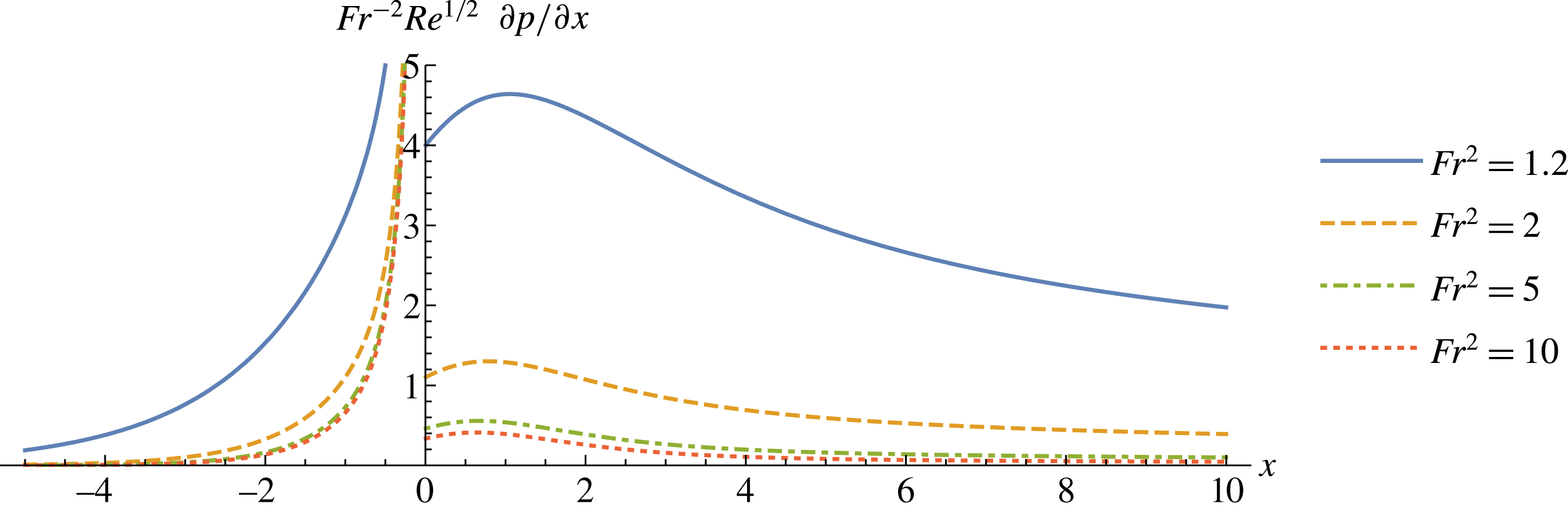
The above discussion is summarised by the plot of
 $\unicode[STIX]{x2202}p^{(1)}/\unicode[STIX]{x2202}x$
in figure 2. In the limit
 $Re\rightarrow \infty$
with
 $Fr>1$
fixed, the induced pressure gradient is bounded for all
 $x>0$
and does not affect the leading-order boundary layer solution. However, this behaviour is not uniform in
 $Fr$
, and in the distinguished limit (3.27), the pressure gradient is large and comparable to the inertia and viscosity terms.


4 Discussion
4.1 Subcritical flows:
$Fr<1$

We have seen that the solution (3.20) has a singularity in the integrand for subcritical flows
 $0<Fr<1$
, because the problem is ill-posed for subcritical incident flows. For such flows, information is capable of propagating arbitrarily far upstream, and it was incorrect to assume that a steady uniform inflow with a given depth and velocity may be imposed.
The singularity in the integrand occurs at the unique positive root
 $k_{\ast }$
to the equation
 $Fr^{2}k=\tanh k$
, suggesting that the perturbation flow
 $w^{(1)}$
should have an oscillatory component
 $\text{e}^{\text{i}k_{\ast }x}$
, corresponding to standing waves of wavenumber
 $k_{\ast }$
for all
 $x$
. There are also travelling waves that would be neglected by a time-independent analysis.
4.2 Boundary layer separation and flow instability
Although the solution (3.20) is non-singular for
 $Fr>1$
, it might not realistically describe the liquid flow. In both of the limits considered in § 3.4, the induced pressure gradient is adverse since
 $\unicode[STIX]{x2202}p/\unicode[STIX]{x2202}x|_{z=0}>0$
. This deceleration of the flow would eventually result in flow reversal and boundary layer separation (Schlichting & Gersten Reference Schlichting and Gersten2003), although the distance downstream at which it would first occur cannot be determined without further consideration of the magnitude of the pressure gradient. The steady flow profile after separation is unstable, and a transition towards turbulence begins there.
The pressure gradient is particularly large for a flow that is only just supercritical, as expressed in the distinguished limit (3.27). It can also be shown that
 $\text{d}h/\text{d}x$
is large in this case. The quickly adjusting depth and the possibility of a flow instability are both features suggestive of a hydraulic jump (Chow Reference Chow1959).
4.3 Non-uniformity in
$x$

In the analysis of § 3, we took
 $x$
to be fixed and
 $O(1)$
whenever
 $Re$
and
 $Fr$
were taken to various limits. The asymptotic solutions that were found are not uniformly valid in
 $x$
. This is because the problem is not uniformly well-posed in
 $x$
.
We noted the singular pressure gradient as
 $x\rightarrow 0^{-}$
. This is caused by the infinite velocity gradient
 $|\unicode[STIX]{x2202}u/\unicode[STIX]{x2202}x|=\infty$
implied by the boundary conditions on
 $z=0$
. This is unrealistic, and the singularity arises because we have neglected the effects of viscosity in the streamwise direction in the region
 $|x|=O(Re^{-1/2})\ll 1$
. This simplification is in common with the classical Blasius solution. Outside this region, the viscous stress in the streamwise direction is dominated by that in the depthwise direction and our previous analysis is still valid.
On the other hand, the assumption that the problem may be divided into an outer flow and a boundary layer, and that the two may be treated separately, becomes invalid when the thickness of the boundary layer is no longer small compared with
 ${\mathcal{H}}$
. The boundary layer has thickness
 $\unicode[STIX]{x1D6FF}(x)\sim Re^{-1/2}(2x)^{1/2}$
, and may no longer be considered to be thin beyond
 $x=O(Re)$
. Moreover, it is not possible to sustain the flow infinitely far downstream of the transition point
 $x=0$
. Indeed, for
 $x\gg 1$
, the inertia terms in (2.2) are
 $O(Fr^{2}/x)$
, while the dominant viscous term is
 $O(Fr^{2}/Re)$
. Hence, beyond
 $x=O(Re)$
, the inertia of the incident flow is no longer sufficient to drive the flow, overcoming basal drag. Again, the solution found in § 3 is invalid beyond
 $x=O(Re)$
.
Although the problem as formulated is unphysical for large
 $x$
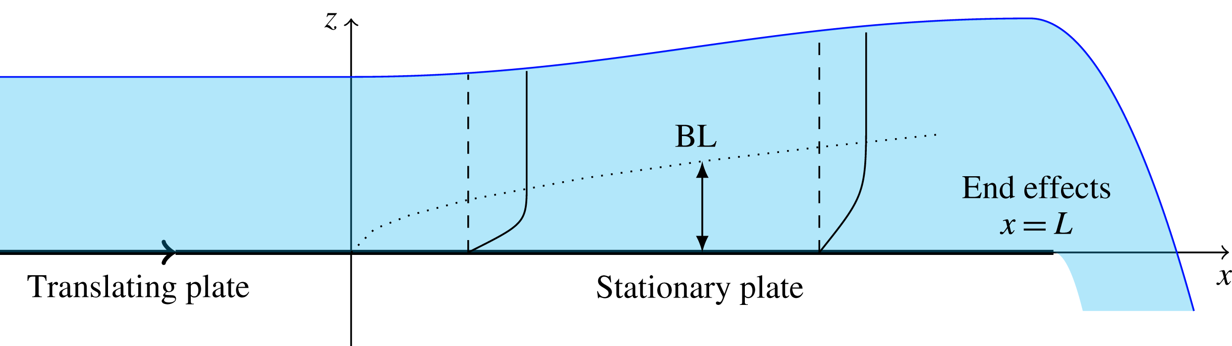
, the analysis given in this work may usefully describe two problems. One possibility is to take the stationary plate as having a finite length
 $L$
, where
 $1\ll L\ll Re$
. If the flow remains supercritical at
 $x=L$
, then the finite length and the details at the trailing edge do not affect the behaviour at
 $x=O(1)$
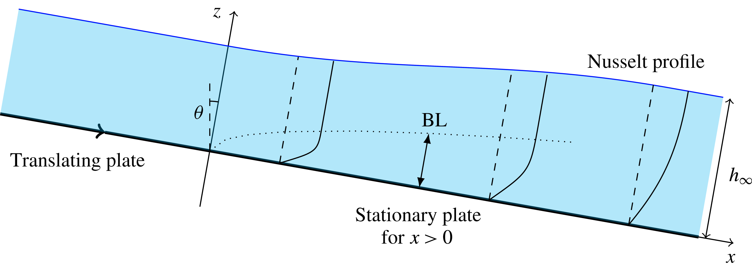
. This problem is sketched in figure 3. Another resolution is to incline the whole system at an angle
 $\unicode[STIX]{x1D703}$
to the horizontal, so that there is a gravitational acceleration
 $g\sin \unicode[STIX]{x1D703}$
in the streamwise direction, as shown in figure 4. The calculations in § 3 are not affected provided that
 $\unicode[STIX]{x1D703}\ll 1$
, such that the streamwise acceleration due to gravity is negligible compared with inertial forces for
 $x=O(1)$
. Beyond
 $x=O(Re)$
, the flow would be governed by a balance between gravity and viscosity, rather than inertia and viscosity. This would result in a Nusselt (semi-Poiseuille) layer flow profile, given by
 $$\begin{eqnarray}\displaystyle u=\frac{Re}{Fr^{2}}\frac{z(2h_{\infty }-z)}{2}\sin \unicode[STIX]{x1D703}, & & \displaystyle\end{eqnarray}$$
where the final depth
 $$\begin{eqnarray}\displaystyle h_{\infty }=\left[\frac{3Fr^{2}q}{Re\sin \unicode[STIX]{x1D703}}\right]^{1/3} & & \displaystyle\end{eqnarray}$$
is determined by conservation of volume flux. In this terminal profile, the effects of viscosity are no longer localised to a bottom boundary layer but have spread throughout the depth of the current.
A plate of finite length
 $1\ll L\ll Re$
. The perturbation solution found in § 3 applies to the region
 $x=O(1)$
but breaks down for
 $x=O(L)$
when end effects become important.

A plate inclined at an angle
 $\unicode[STIX]{x1D703}$
. The effect of streamwise gravity is subdominant for
 $x=O(1)$
provided that
 $\unicode[STIX]{x1D703}\ll 1$
, so that the perturbation solution is valid there. Gravity eventually becomes important and the flow develops into a Nusselt film, with velocity given by (4.1) and depth
 $h_{\infty }$
given by (4.2).

4.4 Applicability to depth-averaged modelling of gravity currents
The problem studied in this work may be viewed as a prototype of a hydraulic flow (here, a free-surface flow driven by gravity) subject to a change in basal topography. In this problem, the change in topography causes a change in the depthwise velocity profile of the current: from an initially uniform profile to one that has a boundary layer governed by viscosity, which grows until eventually at large
 $x$
the effects of viscosity have spread throughout the entire depth of the current, giving the Nusselt film profile (4.1). Chow (Reference Chow1959, chap. 8) described a similar phenomenon when water enters a channel, and the basal roughness of the channel distorts the velocity profile of the flow.
The way in which this velocity profile adjusts would be of interest to those developing depth-averaged descriptions of gravity currents. Such models often use an ad hoc description of the depthwise velocity profile, specified through a shape factor defined by
 $$\begin{eqnarray}\displaystyle \unicode[STIX]{x1D712}=\frac{\overline{u^{2}}}{\overline{u}^{2}}=\frac{\displaystyle h\int _{0}^{h}u^{2}\, d\!z}{\displaystyle \left[\int _{0}^{h}u\, d\!z\right]^{2}}. & & \displaystyle\end{eqnarray}$$
The shape factor is equal to 1 for a uniform flow and to
 $6/5$
for a Nusselt profile. While the simplifying assumption of a uniform flow, with
 $\unicode[STIX]{x1D712}=1$
, is commonly made in the depth-averaged modelling literature (Baker, Johnson & Gray Reference Baker, Johnson and Gray2016), the velocity profile found in the present work gives a more accurate description of
 $\unicode[STIX]{x1D712}$
. Indeed, it can be shown that the perturbation solution from § 3.3 implies that
 $$\begin{eqnarray}\displaystyle \unicode[STIX]{x1D712}=1+cRe^{-1/2}(x/2)^{1/2}H(x)+O(Re^{-1}) & & \displaystyle\end{eqnarray}$$
in the region where that solution is valid (see § 4.3).
An extension of the present work should consider the full evolution of the velocity profile and therefore of the shape factor as
 $x\rightarrow \infty$
, noting the issues discussed in § 4.3. This will give a correction to depth-averaged models of gravity currents in response to topography. Possible applications of this work include the shallow water modelling of avalanches, landslides and debris flows, which are important topics in environmental fluid mechanics, given the damage that such flows can cause (Petley Reference Petley2012).
5 Summary
In this work, we have considered the flow of a low-viscosity fluid layer subject to a sudden change to its basal boundary condition. This change causes a basal boundary layer to form and grow, as in the classical Blasius problem. However, unlike the classical Blasius problem, the fluid in the present problem has finite depth and is bounded above by a free surface.
The presence and growth of the boundary layer displaces the free surface upwards, inducing a streamwise pressure gradient in the outer flow that is not present in the classical problem. We have shown that, as
 $Re\rightarrow \infty$
with
 $Fr>1$
fixed, the induced pressure gradient is
 $O(Fr^{2}Re^{-1/2})$
, which is small compared with the
 $O(Fr^{2})$
inertia and viscosity terms in the boundary layer equation (3.3). Therefore, at leading order, the boundary layer dynamics is the same as in the classical problem: a balance between inertia and viscosity, which is achieved by the Blasius boundary layer profile (3.6). This behaviour is not uniform in
 $Fr$
. The induced pressure gradient may become unbounded as
 $Fr\rightarrow 1$
, and in the distinguished limit (3.27), the pressure gradient is
 $O(1)$
and comparable to the other terms in (3.3).
Acknowledgements
We thank M. Arran, G. Peng, S. J. Cowley and J. Hinch for useful discussions on this work. J.M.F.T. is funded by an EPSRC Studentship (EP/M508007/1) and N.M.V. is a Royal Society Dorothy Hodgkin Research Fellow (DH120121).