





1. Introduction
Nearly a century ago, the zoologist Gray, in an effort to determine the propulsive power of cruising dolphins (Gray Reference Gray1936), stumbled upon a paradox: the drag power of the dolphins exceeds their muscle power. Although it is now considered resolved (see Fish & Lauder Reference Fish and Lauder2006 and Bale et al. Reference Bale, Hao, Bhalla, Patel and Patankar2015), Gray’s paradox had long perplexed researchers studying the hydrodynamics and energetics of swimming fishes, with a singular interest in the mechanics of thrust generation and swimming efficiency. The resolution of the paradox revealed a fundamental aspect of fish propulsion: muscle energy is used to produce lateral undulations that generate thrust, which balances the drag.
In undulatory swimmers, such as eels, the entire body undergoes wave-like motion, and classical analyses by Taylor (Reference Taylor1952) and Lighthill (Reference Lighthill1971) have shown how body-wave kinematics, modal shapes and reactive forces combine to generate thrust and determine swimming speed. However, in fast oscillatory swimmers such as dolphins, lateral movements are primarily confined to the posterior (rear) body, resulting in oscillation of the caudal fin. This observation has led to extensive research on the propulsive characteristics of an oscillating airfoil – a model caudal fin – as an alternative to rotary propellers (Triantafyllou & Barrett Reference Triantafyllou and Barrett1995).
Self-propulsion ensues when the prescribed actuation generates sufficient thrust to overcome the hydrodynamic resistance, establishing a precise balance between the thrust generated and the drag experienced. For a fish cruising at a constant speed, the net force experienced by it must be zero and, therefore, is said to be ‘self-propelling’. Consequently, for self-propelling bodies, a crucial and foundational inquiry arises: What factors determine swimming speed, and how are they influenced by imposed kinematics, such as frequency and amplitude?
Interestingly, oscillating airfoils exhibit a remarkable ability to self-propel, making them simple model systems for investigations of self-propulsion. Across the literature, such studies have employed a wide range of structural assumptions, including fully rigid airfoils (Das et al. Reference Das, Shukla and Govardhan2016), fully flexible airfoils (Alben et al. Reference Alben, Witt, Baker, Anderson and Lauder2012) and configurations with varying rigidity (Gazzola et al. Reference Gazzola, Argentina and Mahadevan2014). Other notable studies on self-propulsion include those of Lauder et al. (Reference Lauder, Anderson, Tangorra and Madden2007), Alben et al. (Reference Alben, Witt, Baker, Anderson and Lauder2012), Das et al. (Reference Das, Shukla and Govardhan2019, Reference Das, Shukla and Govardhan2022), Lagopoulos et al. (Reference Lagopoulos, Weymouth and Ganapathisubramani2019), Liu et al. (Reference Liu, Huang and Lu2020), Wang et al. (Reference Wang, Huang and Lu2020), Gross et al. (Reference Gross, Roux, Raufaste and Médéric2021), Paniccia et al. (Reference Paniccia, Padovani, Graziani and Piva2021), Lin et al. (Reference Lin, Wu and Zhang2021) and Wu et al. (Reference Wu, Shu, Wan, Wang and Chen2022). Although the present work focuses on rigid airfoils, it is essential to acknowledge that flexibility is ubiquitous in aquatic propulsion. It is well established that passive flexibility can play a central role in propulsive performance by introducing rich nonlinear fluid–structure interactions. Studies have shown that thrust generation in flexible panels scale with elastic restoring forces and that peak propulsive efficiency often occurs when the actuation frequency aligns with structural resonance (Dewey et al. Reference Dewey, Boschitsch, Moored, Stone and Smits2013; Moore Reference Moore2014). Alben et al. (Reference Alben, Witt, Baker, Anderson and Lauder2012) have further reported pronounced resonant peaks in the self-propulsion speed of flexible panels. Eloy (Reference Eloy2013) elucidated how the balance of resistive and reactive forces during self-propulsion governs the optimal design of undulatory swimmers. Marais et al. (Reference Marais, Thiria, Wesfreid and Godoy-Diana2012) demonstrated that flexibility can stabilise the wake of a thrust-generating airfoil.
Interestingly, a rigid airfoil which bears little direct morphological resemblance to a fish, exhibits a surprising degree of biological relevance. This relevance is supported by the similarity in scaling laws of macroscopic swimming animals (Gazzola et al. Reference Gazzola, Argentina and Mahadevan2014) and rigid self-propelling airfoils (Das et al. Reference Das, Shukla and Govardhan2016; Lin et al. Reference Lin, Wu and Zhang2021) for Reynolds number
 $O(10^2)$
. Such overlap suggests the existence of similar kinematic mechanisms driving self-propulsion in both rigid airfoils and biological systems. Further, rigid airfoil benefits from the extensive theoretical and experimental understanding of unsteady aerodynamics, which can be more readily translated to self-propulsion. Therefore, characterising the rigid self-propulsion is essential in isolating propulsion mechanisms arising from kinematics from those that depend on passive structural compliance and response.
We emphasise that, in this context, the rigid airfoil is not viewed as a surrogate for biological propulsors in which flexibility is a crucial parameter, but rather as a well-defined and mathematically tractable baseline class of swimmers in its own right. With this baseline established, one may then examine how the deliberate introduction of chord-wise flexibility to a rigid airfoil modifies self-propulsion. Such a coexistence of rigidity and flexibility is characteristic of many fast oscillatory swimmers. Therefore, the choice of rigid airfoils for studying self-propulsion is natural as it is a fundamental problem in unsteady hydrodynamics while being biologically relevant.
In the following subsections, we review the existing literature focusing exclusively on self-propulsion in rigid airfoils, discuss prevailing self-propulsion scaling relations and their limitations, and thereby lay out the necessity, significance and novel contributions of the present experimental study.
1.1. Self-propulsion in rigid airfoils
The spontaneous forward motion of a heaving flat plate and elliptical airfoils first reported by Vandenberghe et al. (Reference Vandenberghe, Zhang and Childress2004) and later by Spagnolie et al. (Reference Spagnolie, Moret, Shelley and Zhang2010) marks an early and systematic exploration of self-propulsion in oscillating airfoils. In both studies, airfoil propulsion occurs beyond a critical frequency, and thereafter the propulsion speed increases linearly with frequency. Numerical simulations of heaving elliptical airfoils (Alben & Shelley Reference Alben and Shelley2005; Zhang et al. Reference Zhang, Liu and Lu2010; Wang et al. Reference Wang, Lin, Zhou and Wu2022), on the contrary report a nonlinear relationship between self-propelling speed and heaving frequency. However, the self-propulsion Reynolds number is
 $O(10^2)$
in numerical simulations, an order of magnitude lower than those studied in the experiments cited earlier.
Purely pitching airfoils form an interesting class of problems in this field. They are simpler to parametrise while still offering valuable physical insight. The quasi-steady circulatory forces due to non-zero angle of attack are purely unsteady since the cycle-averaged angle of attack is zero. Furthermore, when both pitching and heaving motions are involved, the combined motion can often be approximated as pure pitching about a shifted pivot location (Mackowski & Williamson Reference Mackowski and Williamson2017). However, experimental studies on self-propelling pitching airfoils are very limited. Notable contributions include those of Lauder et al. (Reference Lauder, Anderson, Tangorra and Madden2007) on the self-propulsion characteristics of two tandem flapping airfoils and Mackowski & Williamson (Reference Mackowski and Williamson2015) who report the drag-to-thrust transition characteristics at a small pitching amplitude of 2
 $^\circ$
. Although in recent years there has been a growing number of numerical simulations of a pitching airfoil in two-dimensional flow (Das et al. Reference Das, Shukla and Govardhan2016, Reference Das, Shukla and Govardhan2019, Reference Das, Shukla and Govardhan2022; Lin et al. Reference Lin, Wu and Zhang2021; Chao et al. Reference Chao, Jia and Li2024), experimental studies are scarce.
An important result in the numerical studies on self-propulsion in pitching airfoils is the emergence of a scaling relation between the self-propulsion Reynolds number
 $\textit{Re}_s = U_sC/\nu$
and a trailing-edge Reynolds number
 $\textit{Re}_{\textit{TE}} = \textit{fAC}/\nu$
, f is the frequency of pitching (also called ‘flapping Reynolds number’) of the form
 $\textit{Re}_s \sim \textit{Re}_{\textit{TE}}^\alpha$
, where
 $\alpha \gt 1$
. Here,
 $U_s$
is the average self-propulsion speed,
 $C$
is the airfoil chord length,
 $A$
is the total trailing-edge excursion and
 $\nu$
is the kinematic viscosity of the fluid medium. Since
 $A$
is related to pitching amplitude
 $\theta _0$
and pitching location
 $p$
, i.e.
 $A = 2\sin {\theta _0}(1-p)C$
,
 $\textit{Re}_{\textit{TE}}$
is expected to account for all the imposed kinematic parameters. Das et al. (Reference Das, Shukla and Govardhan2016, Reference Das, Shukla and Govardhan2019, Reference Das, Shukla and Govardhan2022) and Lin et al. (Reference Lin, Wu and Zhang2021) report a value of
 $\alpha \approx 5/3$
valid up to
 $\textit{Re}_s \sim O(10^3)$
and
 $\textit{Re}_s \sim O(10^2)$
, respectively. Chao et al. (Reference Chao, Jia and Li2024) report
 $\alpha \approx 4/3$
valid up to
 $\textit{Re}_s \sim O(10^2)$
.
A similar scaling law for macroscopic elastic swimmers with
 $\alpha \approx 4/3$
was reported by Gazzola et al. (Reference Gazzola, Argentina and Mahadevan2014) for
 $\textit{Re}_s \lt O(10^3)$
. Note that the ‘swimming number’ used by Gazzola et al. (Reference Gazzola, Argentina and Mahadevan2014) has the same definition as
 $\textit{Re}_{\textit{TE}}$
except that the trailing-edge excursion
 $A$
is a result of elastic movement of the swimmers and does not reflect the imposed kinematic condition like rigid airfoils. They arrive at these scaling relations by considering a dynamic balance between the average reactive force and skin friction (Gazzola et al. Reference Gazzola, Argentina and Mahadevan2014; Lin et al. Reference Lin, Wu and Zhang2021; Chao et al. Reference Chao, Jia and Li2024) or ‘enhanced skin friction’ (Das et al. Reference Das, Shukla and Govardhan2016, Reference Das, Shukla and Govardhan2019, Reference Das, Shukla and Govardhan2022). The varying
 $\alpha$
values in the scaling relations arise from different assumptions about the drag forces. While these scaling relations are consistent in capturing the effect of frequency on self-propulsion speed, they are, however, inconsistent in accounting for the effect of amplitude. Specifically, Das et al. (Reference Das, Shukla and Govardhan2022) notes the amplitude dependence of the proportionality constant (prominent around
 $\textit{Re}_s \sim O(10^3)$
) of the scaling relation.
Another parameter affecting the propulsive characteristics of a pitching airfoil is the location of the pitching point along the chord. This location has a direct bearing on the net reactive forces and leading-edge suction pressure. In the context of thrust generation, both Tian et al. (Reference Tian, Bodling, Liu, Wu, He and Hu2016) and Mackowski & Williamson (Reference Mackowski and Williamson2017) observe that the net thrust coefficient decreases as the pitching point is shifted from the leading edge to the trailing edge. For self-propelling airfoils, Lin et al. (Reference Lin, Wu and Zhang2019) find that the self-propulsion speed monotonically decreases as the pitch point location is shifted from the leading edge to the trailing edge. Das et al. (Reference Das, Shukla and Govardhan2022) consider a ‘bi-directionally free’ airfoil, i.e. the airfoil is free to move in the forward as well as lateral directions. In such a configuration, the ‘effective pitching point’ location is shifted to the centre of the chord and the self-propulsion speed is lower than the pure-pitching ‘uni-directional’ airfoil. However, similar to amplitude dependence, the proportionality constant in the
 $ \textit{Re}_s-\textit{Re}_{\textit{TE}}$
relation is adjusted to account for the change in effective pitching point. But the exact manner in which the pitching location affects the self-propulsion speed is not quantified. Therefore, the existing single scaling law does not capture the effects of oscillation amplitude and pitching-point location through a single input kinematic parameter,
 $\textit{Re}_{\textit{TE}}$
. This limitation becomes increasingly pronounced at higher Reynolds numbers,
 $\textit{Re}_s \geqslant O(10^3)$
, which are relevant for fast oscillatory swimmers.
Despite the valuable insights gained from numerical investigations, there remains a notable scarcity of experimental results to validate these findings and to resolve discrepancies in reported values of the scaling exponent
 $\alpha$
and in the dependence of
 $\textit{Re}_s$
on oscillation amplitude and pitching point. Furthermore, existing numerical studies are generally restricted to
 $\textit{Re}_s \leqslant O(10^3)$
, and do not encompass the
 $\textit{Re}_s$
range characteristic of biological oscillatory swimmers. Furthermore, biological data for oscillatory swimmers show that the swimming speed increases linearly with frequency at constant tail-beat amplitude (Videler Reference Videler1993; Gazzola et al. Reference Gazzola, Argentina and Mahadevan2014), which reflects as a scaling of the form relation
 $\textit{Re}_s \sim \textit{Re}_{\textit{TE}}$
. In Gazzola et al. (Reference Gazzola, Argentina and Mahadevan2014), the transition from
 $\alpha \approx 4/3$
to
 $\alpha \approx 1$
in
 $\textit{Re}_s \sim \textit{Re}_{\textit{TE}}^{\alpha }$
is accompanied by a transition in drag scaling from viscous to pressure drag for
 $\textit{Re}_s \gt O(10^3)$
. However, the possibility of such a transition in drag scaling and its implications for self-propulsion have not been considered in existing frameworks.
1.2. Objectives of present study
Here, we experimentally investigate the self-propulsion of a sinusoidally pitching rigid airfoil. Our work provides the much-needed experimental database for this problem and addresses the discrepancies in accounting for the effects of amplitude and pitching-point location. In this study, the
 $\textit{Re}_s$
values range from
 $O(10^2)$
to
 $O(10^4)$
, with the upper limit being an order of magnitude higher than those reported in previous studies. We examine the effect of pitching frequency (
 $f$
), amplitude (
 $\theta _0$
) and the location of the pitching point as a fraction of the chord (
 $p$
). To overcome the limitation of a single input parameter
 $\textit{Re}_{\textit{TE}}$
, we assess the impact of the input kinematics through three non-dimensional parameters: frequency Reynolds number (
 $\textit{Re}_{\!f} = (fC)C/\nu$
),
 $\theta _0$
and
 $p$
. We identify not one but three distinct scaling regimes relating
 $\textit{Re}_s$
,
 $\textit{Re}_{\!f}$
,
 $\theta _0$
and
 $p$
through different mechanisms of inviscid thrust and dominant drag which we call the power, separable and linear scaling regimes.
An important contribution of this work is the identification of the separable and linear regimes for the self-propelling pitching airfoil, which has not been reported earlier. They retain the linear relationship between self-propulsion speed and frequency observed in oscillatory swimmers (Videler Reference Videler1993; Gazzola et al. Reference Gazzola, Argentina and Mahadevan2014) and explicitly account for amplitude and pitching-point locations. We also observe different vortical patterns in the wake along with the reverse Kármán wake. These vortical patterns are correlated not only to the Strouhal number (
 $\textit{St}$
) but also depend on the normalised distance travelled by the airfoil in one oscillation cycle,
 $U^*_{\textit{BL}}$
. A reverse Kármán vortex street is seen only when
 $\textit{St} \leqslant 0.4$
and
 $0.4 \lt U^*_{\textit{BL}} \lt 1$
, corresponding the ranges of
 $\textit{St}$
and
 $U^*_{\textit{BL}}$
for biological oscillatory swimmers. To the best of our knowledge, this is the first experimental work to systematically explore all three pitching parameters and explicitly establish their individual effects on self-propulsion speed.
In this article, we first discuss the experimental set-up used to achieve self-propulsion and the range of parameters explored in § 2 . In §§ 3 and 4, we discuss in detail how the self-propulsion speed varies with the imposed kinematics, how and why
 $\textit{Re}_{\textit{TE}}$
is inadequate and how the three scaling relations emerge. In § 5, we present the different wake patterns and discuss how the wake pattern relates to
 $\textit{St}$
and
 $U^*_{\textit{BL}}$
and how the two parameters together determine biological relevance. Section 6 concludes the article while summarising key findings.
2. Experimental methodology
We use a NACA0015 airfoil section with chord length
 $C = 38.9 \, \mathrm{mm}$
and span
 $h = 100.1\, \mathrm{mm}$
. The airfoil is made with acrylonitrile butadiene styrene by vacuum casting. The density of the airfoil is
 $1.01 \, \mathrm{g\,cm}^{-3}$
, ensuring the airfoil is close to being neutrally buoyant. Details of the airfoil fabrication process can be found in Shinde (Reference Shinde2012). The airfoil is fully submerged such that the mid-chord is at a depth of
 $10\,\mathrm{cm}$
from the water surface while the upper end of the airfoil is 5 cm deep. The airfoil propels in a large water tank measuring
 $2\,\mathrm{m} \times 1\,\mathrm{m} \times 0.5\,\mathrm{m}$
. We use a rotary apparatus, similar to the ‘merry-go-round’ set-up of Thiria & Godoy-Diana (Reference Thiria and Godoy-Diana2010), to achieve self-propulsion. An important distinction in our set-up is the use of a long arm to prevent multiple arm rotations before the airfoil achieves self-propulsion. Figure 1 schematic shows the schematic of the top view of the apparatus. The airfoil is positioned at the end of a long, freely rotating arm with an effective length of
 $R = 1.04\,\mathrm{m} (\gt 20C)$
. Between the start and stop positions, the arm is free to rotate for approximately
 $120^\circ$
, resulting in a path length of approximately
 $2\,\mathrm{m}$
. The total travel distance exceeds the straight-line distance between the two endpoints because of this curved trajectory.
(a) Schematic of the top view of the apparatus. The red-dashed line indicates the path traversed by the airfoil. (b) Side view of the airfoil assembly. (c) The position–time graph shows the airfoil’s instantaneous position over time during pitching at
 $2\,\mathrm{Hz}$
with an amplitude of
 $9.5^\circ$
. The slope of the linear fit is the self-propelling velocity. (d) Side view of the motor and bearing assembly showing the freely rotating shaft supported by air bearings.

The rotating arm is a truss structure fabricated in-house with carbon fibre. This truss (rotating arm) is securely mounted on a high-precision steel shaft. The shaft is supported by a combination of axial and thrust (flat) air bearings (figure 1). The bearings allow free rotation of the shaft and the truss while constraining motion in other directions. The use of air bearings ensures that the friction from the supporting structure is negligible. A DC motor is mounted near the shaft, while the batteries required to power the motor and the controllers are mounted as a counterweight (figure 1). A spiral-spring-based crank–rocker mechanism converts rotary motion into sinusoidal oscillation and transmits it over a long distance. The rocker of the mechanism is connected to the airfoil through a spiral power spring;
 $M3 \times 20\,\mathrm{mm}$
threaded holes are positioned along the chord line to allow for adjustments in the pitching-point location. The airfoil is connected to the spiral spring through a pair of ball bearings. This connecting shaft has a diameter of
 $3\,\mathrm{mm}$
.
We use an incremental magnetic rotary encoder (Renishaw©LM10) with an angular resolution of
 $0.018^\circ$
to measure the instantaneous position of the shaft. The encoder is directly mounted on the shaft itself (see figure 1). The linear resolution of the position measured at the airfoil end is
 $\approx 0.007C$
. The position–time plot in figure 1(c) shows the typical measured linear position with time for a representative case. The steady self-propelling state of the airfoil is identified as a linear region in the position–time curve. A linear function is fitted to the data within this region. The slope of this linear segment, averaged across
 $120{-}150$
oscillation cycles (in
 $10{-}15$
trials), is reported as the self-propelling speed
 $U_s$
. The nature of this position–time curve is similar across all cases, except for variations in the time required to achieve self-propulsion and the slope of the linear region. The typical deviation in
 $U_s$
across the trials was less than 2 % for
 $U_s\gt 10$
cm s−1 but increased to 10 % when
 $U_s \lt 3$
cm s−1. A more detailed discussion of the apparatus focused on the mechanism’s kinematics and the characterisation of self-propulsion can be found in Joshi & Arakeri (Reference Joshi and Arakeri2022, Reference Joshi and Arakeri2024).
We use the laser-induced fluorescence (LIF) technique to observe vortex patterns in the wake. A 532 nm continuous laser sheet illuminates the mid-span of the airfoil near the centre of the water tank. In this region, the airfoil is already in a self-propelling state (figure 1) for all the parameters. Rhodamine B solution is continuously injected from a small reservoir (with a 5 ml capacity) near the airfoil end. A thin tube connects the reservoir to the dye injection port on the airfoil located at
 $p = 0.2$
. This port opens at mid-span. The dye is released smoothly onto the airfoil surface through a porous plug. The dye flow rate is adjusted for each propulsion speed and tested by towing the airfoil at different speeds. Instantaneous images of the flow field are captured using a high-speed camera.
Illustration of the NACA0015 airfoil section with depictions of the trailing-edge excursion on the left and the locations of pitching points on the right. The pitching locations P1, P2 and P3 are at
 $p = 0.125$
,
 $p = 0.3$
and
 $p = 0.48$
, respectively.

2.1. Parametric space
We pitch the airfoil sinusoidally such that the instantaneous pitch angle of the airfoil is given by
 $\theta =\theta _0 \sin (2\pi ft)$
. We consider four different amplitude values:
 $\theta _1 \approx 4.6^\circ$
,
 $\theta _2 \approx 9.4^\circ$
,
 $\theta _3 \approx 14.8^\circ$
and
 $\theta _4 \approx 20.5^\circ$
. The selection of these amplitude values ensures comparability with existing numerical studies in the literature and is expected to capture essential unsteady aerodynamics (Lin et al. Reference Lin, Wu and Zhang2021; Das et al. Reference Das, Shukla and Govardhan2022). Furthermore, the total trailing-edge excursion of the airfoil when pitched at
 $\theta _1$
and
 $\theta _2$
is comparable to the tail-beat amplitude in oscillatory swimmers (Videler Reference Videler1993). While these two amplitudes are more relevant from a fish swimming perspective, the higher amplitudes
 $\theta _3$
and
 $\theta _4$
are interesting from the unsteady aerodynamics perspective. Note that the exact pitching amplitude achieved by the mechanism has a weak dependence on the pitching frequency. This dependence arises from unavoidable friction between coils inside the power spring used in the mechanism for sinusoidal actuation (Joshi & Arakeri Reference Joshi and Arakeri2024). Therefore, we measure the actual pitching amplitude through a series of high-speed images and use this value in all calculations. However, we refer to the average values of
 $\theta _0$
for ease of communication.
The location of the pitching point
 $p$
represents the location as a fraction of the airfoil chord. As such,
 $p = 0$
at the leading edge and
 $p = 1$
at the trailing edge. Therefore, when pitched at
 $p$
, the actual distance of the pitching point is
 $pC$
from the leading edge. In the present work, we consider three pitching points – P1, P2 and P3 – at
 $p = 0.125, 0.3$
and
 $0.48$
, respectively. All the geometric parameters and the pitching-point locations are sketched in figure 2. Here, P1 is closest to the leading edge where both aerodynamic and reactive forces contribute significantly to thrust. P2 is close to the aerodynamic centre where the thrust contribution is mainly from reactive forces. This pitching location is used across the bulk of the existing pitching airfoil literature. P3 is near mid-chord where thrust is generated solely by the aerodynamic force while the reactive forces’ contribution is nearly zero. A detailed discussion on the effect of pitching-point location on these forces based on linear inviscid theory of Garrick (Reference Garrick1936) is presented in § 4. However, pitching locations beyond the mid-chord were excluded because they are associated with significant thrust decay (Mackowski & Williamson Reference Mackowski and Williamson2017) and pose substantial structural stability challenges in connecting the airfoil to the actuating mechanism due to the decreasing thickness of the NACA0015 profile.
The pitching frequency is varied from
 $0.25 \, \mathrm{}$
to
 $8 \, \mathrm{Hz}$
, depending on the amplitude and pitching point. The range of frequency is also the typical range of caudal fin oscillations in oscillatory swimmers. For a given amplitude and pitch location, the lowest frequency is the one at which self-propulsion is reliable and repeatable across trials. The largest frequency is limited by the occurrence of water sloshing and/or transverse (spanwise) oscillations of the truss. The self-propulsion speed ranges from approximately 2 to
 $45 \, \mathrm{cm\,s}^{-1}$
, with the corresponding
 $\textit{Re}_s$
values ranging from
 $400$
to
 $17\,000$
, spanning two orders of magnitude.
2.2. Operational design considerations and constraints
The experimental design ensures that finite-span effects, tank-wall proximity and the curved trajectory of the airfoil do not significantly influence the self-propulsion dynamics. However, free-surface proximity and the large lateral forces generated by the airfoil remain important constraints that limit the range of pitching frequencies explored. Below, we describe how each of these factors is accounted for and discuss their impact on our findings.
The finite span of the airfoil does not significantly influence its self-propulsion characteristics. This is supported by the close agreement of our measurements with two-dimensional numerical simulations (Das et al. Reference Das, Shukla and Govardhan2016) and with experiments employing end plates to enforce a nominally two-dimensional flow (Mackowski & Williamson Reference Mackowski and Williamson2015) (discussed later in § 4). Furthermore, the consistency of our results with theoretical predictions derived under two-dimensional assumptions indicates that the flow in the vicinity of the airfoil and in the immediate downstream region is predominantly two-dimensional. Two-dimensionality of the flow around the airfoil is further supported by the experimental findings of Buchholz & Smits (Reference Buchholz and Smits2008), who showed that the thrust coefficient of a finite-aspect-ratio pitching airfoil without end plates is independent of aspect ratio for values greater than one and matches that of a pitching airfoil with end plates. Finite-span effects, however, do influence downstream wake evolution. Approximately one chord length downstream of the airfoil, the wake widens noticeably. This behaviour is consistent with the wake evolution model of Buchholz & Smits (Reference Buchholz and Smits2008) for finite airfoils, which describes the interactions between spanwise and streamwise vorticity. However, this downstream wake evolution does not influence the near-field flow and, therefore, the forces acting on the airfoil.
In the self-propulsion state, the airfoil is located more than
 $10C$
from the tank walls, ensuring negligible wall influence. The airfoil is released from rest at a position at least
 $2C$
from the tank wall. Even when the airfoil is released from a distance less than
 $1C$
from the tank wall, we observe that the wall proximity influences only the initial acceleration phase and does not affect the steady self-propulsion speed. Similarly, the airfoil’s stopping point is always at least
 $2C$
from the tank walls. Here, allowing the airfoil to continue travelling toward a wall boundary did not change the measured steady speed.
Although the airfoil travels along a circular arc, curvature effects can be neglected and the propulsion treated as locally rectilinear. The following arguments support this approximation. First, the geometric curvature is small: the ratio of chord length to rotating arm radius is
 $C/R \approx 0.037 \ll 1$
. The associated average thrust lost in turning is therefore estimated to be below
 $4\,\%$
. Second, the ratio of the angular speed due to arm rotation (
 $U_s/R$
) to the pitching frequency (
 $2\pi f$
) is
 $O(10^{-2})$
–
 $O(10^{-3})$
across all cases, meaning that pitching occurs at least two orders of magnitude faster than the turning motion. Lastly, the ratio of centripetal to hydrodynamic forces on the airfoil scales as
 $t_a/R \sim O(10^{-3})$
when the airfoil density matches that of the surrounding fluid. Here,
 $t_a$
is the airfoil thickness. The wake deflection observed in some cases (§ 5) is not an artefact of path curvature, as the wake deflects to either side within a given trial. If the curvature effect influenced deflection, it would consistently occur in a single direction. Moreover, wake deflection is expected for pitching airfoils for
 $\textit{St}\gt 0.4$
, and our observations are consistent with prior reports of this behaviour (§ 5).
We noted earlier that although the airfoil is fully submerged, the upper edge of the airfoil is only 5 cm below the surface (
 $\approx 1.3 C$
) where potential interaction with the water surface is possible, particularly at large pitching amplitudes. This interaction is further complicated by a 3 mm-diameter cylindrical support rod that pierces the free surface to connect the airfoil to the actuation mechanism. It behaves as a cantilever beam and experiences significant transverse loading. A trade-off exists in selecting the submergence depth. Increasing depth reduces free-surface interaction but requires a longer support rod, which increases transverse loading and drag. Because these effects cannot be independently controlled, we experimentally varied the submergence depth (Joshi & Arakeri Reference Joshi and Arakeri2022). The measured self-propulsion speed remained mostly constant or decreased slightly with increasing depth, with variations within experimental uncertainty. In Joshi & Arakeri (Reference Joshi and Arakeri2022), we further quantified the cumulative resistance to self-propulsion from the apparatus, noting that their combined contribution is marginal and comparable to measurement uncertainty. However, for large pitching amplitudes (
 $\theta _3$
and
 $\theta _4$
) and for frequencies beyond 6 Hz, the coupled free-surface interaction and structural response produce transverse oscillations of the rotating arm and noticeable surface sloshing. For a given
 $p$
and
 $\theta _0$
, these effects limit the maximum frequency that can be explored. At the threshold frequency, the transverse arm oscillations cause the laser light sheet, nominally aligned with the airfoil mid-plane, to deviate by more than the sheet thickness (2–3 mm). In addition, the self-propulsion speed decreases with an increase in frequency beyond this threshold (Joshi Reference Joshi2025). This frequency threshold decreases with increasing amplitude, indicating that the transverse oscillations are due to a combined effect of large normal forces and free-surface interactions and not due to structural resonance.
3. Self-propulsion speed
We introduced in § 1 the use of
 $\textit{Re}_{\textit{TE}}$
as a single parameter used to determine self-propulsion characteristics. In the expression
 $\textit{Re}_{\textit{TE}} = \textit{fA} C / \nu$
, the term
 $ \textit{fA}$
is a trailing-edge velocity scale. Therefore,
 $\textit{Re}_{\textit{TE}} = U_{\textit{TE}} C / \nu$
, where
 $U_{\textit{TE}} = \textit{fA}$
. This definition of
 $U_{\textit{TE}}$
accounts for all three pitching parameters since
 $A = 2\sin {\theta _0}(1-p)C$
. In figures 3(a) and 3(b), we plot
 $U_s$
with trailing-edge velocity,
 $U_{\textit{TE}} = \textit{fA}$
, and
 $\textit{Re}_s$
with
 $\textit{Re}_{\textit{TE}}$
, respectively. The error in measurement, defined as twice the standard deviation, is less than the symbol size. Note that we did not observe any self-propulsion when pitched at P3 with amplitude
 $\theta _1$
.
For a given pitching point,
 $U_s$
(and
 $\textit{Re}_s$
) increases with
 $U_{\textit{TE}}$
(and
 $\textit{Re}_{\textit{TE}}$
) (figure 3). The
 $U_s$
value ranges from approximately
 $2 \,\mathrm{cm\,s}^{-1}$
to nearly
 $45\,\mathrm{cm\,s}^{-1}$
for pitching location P1,
 $26\,\mathrm{cm\,s}^{-1}$
for P2 and
 $10\,\mathrm{cm\,s}^{-1}$
for P3. In general, we observe larger
 $U_s$
values for P1, with speed decreasing as the pitching point is moved closer to the centre (P3). The
 $\textit{Re}_s$
value varies from approximately 400 to 17 000 for
 $\textit{Re}_{\textit{TE}}$
in the range 200–5000. Note that, although both the panels in figure 3 differ only by a constant scaling factor, the wide range of
 $\textit{Re}_s$
values masks the amplitude dependence in
 $U_s$
. Therefore, inclusion of both linear and logarithmic plots emphasises the need to assess dimensional and non-dimensional quantities in their own merit. Furthermore, figure 3(b) also presents the overall range of Reynolds number for self-propulsion enabling useful comparison with other studies in the literature.
We observe that the dependence of
 $U_s$
(and
 $\textit{Re}_s$
) on pitching-point location and amplitude is not well captured by
 $U_{\textit{TE}}$
(and
 $\textit{Re}_{\textit{TE}}$
);
 $U_s$
still exhibits amplitude and pitching-point dependence for pitching locations P1 and P2. Only for P3 do we see a linear increase in
 $U_s$
with
 $U_{\textit{TE}}$
, with all the points collapsing on a straight line;
 $U_{\textit{TE}}$
, and therefore
 $\textit{Re}_{\textit{TE}}$
, although a function of
 $\theta _0$
and
 $p$
, cannot adequately capture their individual effects on self-propulsion for pitching locations P1 and P2.
Variation of the self-propelling velocity
 $U_s$
with
 $U_{\textit{TE}}$
(a) and the self-propulsion Reynolds number
 $\textit{Re}_s$
with trailing-edge Reynolds number
 $\textit{Re}_{\textit{TE}} = \textit{fAC}/\nu$
(b) for all the parameters studied. Solid lines (b) represent the best fit.

The inadequacy of
 $U_{\textit{TE}}$
as a single input parameter is more clearly understood when comparing the variation in self-propulsion reduced frequency
 $k_s = \pi fC/U_s$
and speed in terms of body lengths per oscillation
 $U^*_{\textit{BL}} = U_s/fC$
. The value of
 $U^*_{\textit{BL}}$
represents the normalised distance travelled by the airfoil in an oscillation cycle;
 $k_s$
is a widely used parameter in unsteady aerodynamics, while
 $U^*_{\textit{BL}}$
is commonly used to compare the swimming speed of different oscillatory swimmers (Videler Reference Videler1993). By definition,
 $U^*_{\textit{BL}}$
is related to the inverse of the self-propelling reduced frequency
 $k_s$
such that
 $U^*_{\textit{BL}}={\pi }/{k_s}$
. In figures 4(a) and 4(b) we plot
 $k_s$
and
 $U^*_{\textit{BL}}$
with pitching amplitude
 $\theta _0$
for different
 $p$
. Note that
 $\theta _0$
values are considered in radians for all calculations.
From figure 4(a), we observe a wide range of
 $k_s$
values, from
 $1$
to
 $22$
, indicating a considerable variation in the degree of unsteadiness across all parameters. This variation is particularly prominent for pitching location P3. For pitching locations P1 and P2, the variation in
 $k_s$
is significant when
 $\theta _0 \lt 0.1$
rad (
 $\theta _1$
). For
 $\theta _0\gt 0.1$
rad (
 $\theta _2, \theta _3, \text{ and } \theta _4$
), points corresponding to different frequencies cluster closely together for nearly the same
 $\theta _0$
, indicating a linear dependence of self-propulsion speed on frequency. In figure 4(b), the data points for each pitching point are along a single curve and
 $U^*_{\textit{BL}}$
increases as the pitching point approaches the leading edge, i.e. as
 $p$
decreases. The maximum value of
 $U^*_{\textit{BL}}\approx 2$
occurs when pitching closest to the leading edge (P1 with
 $p = 0.125$
) for pitching amplitude
 $\theta _4$
. The value of
 $U^*_{\textit{BL}}$
increases monotonically with
 $\theta _0$
. However, for pitching points P1 and P2 and
 $\theta _0 \gt 0.14$
rad, the rate at which
 $U^*_{\textit{BL}}$
increases with
 $\theta _0$
reduces, indicating reduced sensitivity to further increase in amplitude. This diminishing effect of amplitude on self-propulsion reflects a change in the dominant drag mechanism (discussed in § 4) during self-propulsion and is more pronounced in the
 $k_s$
vs
 $\theta _0$
plot (figure 4
a). For pitching amplitudes
 $\theta _2$
,
 $\theta _3$
and
 $\theta _4$
(
 $\theta _0 \gt 0.14$
rad) the variation of
 $k_s$
with
 $\theta _0$
is well captured by the relation
 $k_s \sim \theta _0^{-1/2}$
for pitching locations P1 and P2 and
 $k_s \sim \theta _0^{-1}$
for P3. The inverse square root dependence of
 $k_s$
on
 $\theta _0$
indicates that the
 $U_s$
increases only as
 $\theta _0^{1/2}$
, an effect not captured by
 $U_{\textit{TE}}$
.
The inadequacy of
 $U_{\textit{TE}}$
as a single parameter for characterising the input kinematics arises because it is not tied to the physical mechanisms responsible for thrust generation, but instead follows directly from geometric considerations influencing wake width. In the definition of
 $U_{\textit{TE}}$
, and consequently
 $\textit{Re}_{\textit{TE}}$
, the characteristic velocity scale is based solely on the total trailing-edge excursion
 $A$
, which is assumed to influence the wake width. Although
 $A$
depends on
 $p$
and
 $\theta _0$
, this dependence does not reflect the manner in which the primary thrust-generating and drag mechanisms scale with
 $p$
and
 $\theta _0$
. The dominant inviscid contributions to the mean thrust originate from reactive forces and leading-edge suction, whose dependence on
 $p$
differs substantially from that implied by
 $A$
. A transition from viscous to pressure drag further changes the drag dependence on
 $\theta _0$
. In subsequent sections, we discuss these aspects in detail and explore the effects of
 $f$
,
 $\theta _0$
and
 $p$
explicitly without combining them in
 $U_{\textit{TE}}$
(and
 $\textit{Re}_{\textit{TE}}$
).
At this point, it is useful to revisit the biological relevance of the present study. The examination of steady-state swimming in oscillatory swimmers across different species reveals that the normalised speed
 $U^*_{\textit{BL}}$
is between
 $0.2$
and
 $0.8$
(Videler Reference Videler1993; Gazzola et al. Reference Gazzola, Argentina and Mahadevan2014) while some high-speed swimmers can go up to
 $U^*_{\textit{BL}} \approx 1.2$
(Gazzola et al. Reference Gazzola, Argentina and Mahadevan2014). Their tail-beat excursion is within the range of
 $10\,\% {-} 30\,\%$
of their body length (Videler Reference Videler1993; Gazzola et al. Reference Gazzola, Argentina and Mahadevan2014). Similar values of trailing-edge excursion are achieved for a rigid pitching airfoil when pitching at
 $\theta _1$
and
 $\theta _2$
. For these amplitudes,
 $U^*_{\textit{BL}}$
is also in the range 0.2–1.3 (figure 4), which is same as oscillatory swimmers.
Self-propulsion reduced frequency
 $k_s = \pi fC/U_s$
(a) and non-dimensional speed
 $U^*_{\textit{BL}} = U_s/fC$
(b) with pitching amplitude
 $\theta _0$
in radians. Note that
 $U^*_{\textit{BL}} = \pi /k_s$
. In (b), the range of
 $U^*_{\textit{BL}}$
for oscillatory swimmers Videler (Reference Videler1993), Gazzola et al. (Reference Gazzola, Argentina and Mahadevan2014) is indicated with red-dashed lines.

4. Scaling regimes
To independently assess the effect of all the pitching parameters, we define a frequency Reynolds number
 $\textit{Re}_{\!f} = (fC)C/\nu$
, where the longitudinal velocity scale
 $fC$
depends only on the pitching frequency and explore the effect of
 $\textit{Re}_{\!f}$
,
 $\theta _0$
and
 $p$
on
 $\textit{Re}_s$
. We discuss the dominant thrust and drag mechanisms, how the three scaling regimes emerge from these mechanisms and validate these relations with our experimental data.
4.1. Thrust generation as an inviscid phenomenon
For a thrust-generating airfoil oscillating in a uniform free stream, the instantaneous net propulsive thrust coefficient
 $C_T$
consists of an average and an unsteady component
 \begin{equation} C_T = \bar {C_T} + C_{T0}\sin {(2\omega t + \phi )}. \end{equation}
Here,
 $\bar {C_T}$
is the average thrust coefficient,
 $C_{T0}$
is the amplitude of the unsteady component,
 $\omega = 2\pi f$
is the angular frequency and
 $\phi$
is the phase difference between the propulsive thrust and the sinusoidal oscillation of the airfoil. Mackowski & Williamson (Reference Mackowski and Williamson2015) found that the measured
 $C_{T0}$
and
 $\phi$
values matched very well with the values predicted by the linear inviscid theory of Garrick (Reference Garrick1936). Their finding established that the thrust generated by a pitching airfoil is primarily due to inviscid mechanisms well captured by the linear inviscid theory of Theodorsen (Reference Theodorsen1935) and Garrick (Reference Garrick1936). An important consequence of these findings is that the average thrust
 $\bar {C_T}$
can now be determined by offsetting the inviscid average thrust
 $\bar {C}_{T,\textit{in}}$
with a suitable average drag coefficient
 $\bar {C}_D$
, i.e.
 \begin{equation} \bar {C_T} = \bar {C}_{T,\textit{in}} - \bar {C}_D. \end{equation}
In a self-propelling state,
 $\bar {C}_T = 0$
. Therefore,
 $\bar {C}_D = \bar {C}_{T,\textit{in}}$
.
The linear inviscid thrust (
 $\bar {C}_{T,\textit{in}}$
) is a linear superposition of the reactive thrust (
 $\bar {C}_{\!R}$
), circulatory thrust (
 $\bar {C}_C$
), including the induced circulation due to wake vorticity, and leading-edge suction (
 $\bar {C}_{Les}$
). As such
 \begin{equation} \bar {C}_{T,\textit{in}} = \bar {C}_{\!R} + \bar {C}_C + \bar {C}_{\textit{LeS}}. \end{equation}
In Appendix A, we revisit the inviscid theory (Garrick Reference Garrick1936) to derive the expressions for
 $\bar {C}_{\!R},\bar {C}_C,\bar {C}_{\textit{LeS}}$
and
 $\bar {C}_{T,\textit{in}}$
as functions of reduced frequency
 $k = \pi fC/U$
for a pitching flat-plate airfoil in a uniform free stream. In the limit
 $k \rightarrow \infty$
,
 $\bar {C}_{T,C} \approx 0$
while
 \begin{equation} \bar {C}_{\!R} = \pi \theta _0^2\frac {k^2}{2}\left (1-2p\right )\!, \end{equation}
and
 \begin{equation} \bar {C}_{\textit{LeS}} \approx \pi \theta _0^2 \frac {k^2}{4} \left ( 2p - \frac {1}{2} \right )^2 \!, \end{equation}
with the total inviscid thrust
 \begin{equation} \bar {C}_{T,\textit{in}} \approx \pi \theta _0^2\frac {k^2}{4}\left (\frac {3}{2} -2p\right )^2 \!. \end{equation}
Since all the thrust coefficients scale as
 $\pi \theta _0^2k^2/2$
, we assess the effect of the pitching-point location on the normalised thrust coefficients
 $\bar {C}_{\!R}^* = \bar {C}_{\!R}/(\pi \theta _0^2k^2/2)$
,
 $\bar {C}_{\textit{LeS}}^* = \bar {C}_{\textit{LeS}}/(\pi \theta _0^2k^2/2)$
and
 $\bar {C}_{T,\textit{in}}^* = \bar {C}_{T,\textit{in}}/(\pi \theta _0^2k^2/2)$
.
In figure 5 we plot the variations of
 $\bar {C}_{\!R}^*$
,
 $\bar {C}_{\textit{LeS}}^*$
,
 $\bar {C}_{T,\textit{in}}^*$
with the pitching-point location. We also plot the variation of fractional contributions
 $ \bar {C}_{\!R}/\bar {C}_{T,\textit{in}}$
and
 $ \bar {C}_{\textit{LeS}}/\bar {C}_{T,\textit{in}}$
with pitching-point location. The reactive thrust is positive when
 $p\lt 1/2$
and negative when
 $p\gt 1/2$
with
 $\bar {C}_{\!R}^*$
decreasing linearly with
 $p$
. At
 $p = 1/2$
,
 $\bar {C}_{\!R} = 0$
. The contribution of leading-edge suction to the total inviscid thrust is zero when pitched at
 $p = 1/4$
, but positive at all other locations. We see larger values of
 $\bar {C}_{\textit{LeS}}^*$
at the trailing-edge side of the airfoil beyond
 $p\gt 1/2$
. At three-quarter chord, i.e.
 $p = 3/4$
, the negative reactive thrust is balanced by the positive leading-edge suction, resulting in zero average thrust. Nevertheless, for
 $p\lt 1/2$
,
 $\bar {C}_{\textit{LeS}}^*$
values are much smaller compared with
 $\bar {C}_{\!R}^*$
. The total thrust is dominated by reactive forces until
 $p\approx 0.4$
, evident from the variation of
 $\bar {C}_{\!R}/\bar {C}_{T,\textit{in}}$
with
 $p$
in figure 5. Therefore, for pitching locations with
 $p\lt 0.4$
, the total inviscid thrust scales as the reactive thrust itself, such that
 \begin{equation} \bar {C}_{T,\textit{in}} \sim \bar {C}_{\!R} \sim \theta _0^2 k^2(1-2p). \end{equation}
However, when pitched close to the mid-chord (
 $p \approx 1/2$
), the thrust generation would be due to leading-edge suction such that
 \begin{equation} \bar {C}_{T,\textit{in}} \sim \bar {C}_{\textit{LeS}} \sim \theta _0^2k^2. \end{equation}
In figure 6 we compare the variations of
 $\bar {C}_{\!R},\bar {C}_C$
,
 $\bar {C}_{\textit{LeS}}$
and
 $\bar {C}_{T,\textit{in}}$
, normalised by
 $\pi \theta _0^2$
, with
 $k$
for pitching locations P1 (
 $p = 0.125$
), P2 (
 $p = 0.3$
) and P3 (
 $p = 0.48$
). Note that
 $C^\#_R = \bar {C}_{\!R}/\pi \theta _0^2$
,
 $C^\#_C = \bar {C}_C/\pi \theta _0^2$
,
 $C^\#_{\textit{LeS}} = \bar {C}_{\textit{LeS}}/\pi \theta _0^2$
and
 $C^\#_{T,\textit{in}} = \bar {C}_{T,\textit{in}}/\pi \theta _0^2$
. We see that the asymptotic behaviour of
 $\bar {C}_{T,\textit{in}}$
from (4.7) (for P1 and P2) and (4.8) (for P3) derived in the limit of
 $k \rightarrow \infty$
is valid for
 $k\gt 1$
and
 $k \gt 5$
, respectively. Recall from our earlier discussions and figure 4 that the measured
 $k_s$
values are within the range of validity of these asymptotic relations.
Inviscid thrust coefficients normalised by
 $\pi \theta _0^2k^2/2$
(a) and their relative contribution to the total thrust (b) as a function of pitching-point location
 $p$
in the asymptotic limit of
 $k \rightarrow \infty$
. Refer to colour version for legend.

The variation of inviscid thrust coefficients normalised by
 $\pi \theta _0^2$
with reduced frequency
 $k$
for the pitching locations examined in the experiments. Here, the total average inviscid thrust coefficient is in black, reactive forces is in red, circulatory forces is in green and leading-edge suction is in blue. Refer to the colour version.

Three scaling regimes: (a) power scaling regime for
 $\theta _1$
and pitching locations P1 and P2 compared with Mackowski & Williamson (Reference Mackowski and Williamson2015) and Das et al. (Reference Das, Shukla and Govardhan2016) for
 $p = 0.25C$
and
 $\theta _0 = 2^{\circ}$
and
 $\theta _0 = 2^{\circ}$
, respectively; (b) separable scaling regime for
 $\theta _2,\theta _3$
and
 $\theta _4$
and pitching location P1 and P2 and with data points from Das et al. (Reference Das, Shukla and Govardhan2022) collapsing much better with (4.15); (c) linear scaling regime when pitched at P3. The inset in (c) shows the same relation in a linear plot. Legend is same as figure 3.

4.2. Power scaling regime
When pitching at
 $\theta _1$
(
 $\theta _0 \approx 4.6^\circ$
), viscosity is expected to influence self-propulsion and the impact of skin friction on self-propulsion would be significant. Moreover, the presence of a moving airfoil surface further enhances skin friction in accordance with the Bone–Lighthill boundary-layer thinning hypothesis (Lighthill Reference Lighthill1971). While the boundary-layer skin friction scales as
 $\textit{Re}^{-1/2}$
for laminar flow over stationary boundary, it increases as
 $\textit{Re}^{-1/2}|U^*_n|^{1/2}$
for moving surfaces (Ehrenstein et al. Reference Ehrenstein, Marquillie and Eloy2014), where
 $U^*_n$
represents a non-dimensional normal velocity. For a pitching airfoil,
 $U^*_n \sim k_s\theta _0$
. Consequently, for the self-propelling airfoil, the cycle-averaged drag coefficient
 $\bar {C_D}$
would then scale as
 \begin{equation} \bar {C_D} \sim \textit{Re}_s^{-1/2}(k_s \theta _0)^{1/2}. \end{equation}
Equating (4.7) and (4.9) we get
 \begin{equation} \textit{Re}_s^{-1/2} \sim (1 -2p)k_s^{3/2}\theta _0^{3/2}. \end{equation}
Since
 $k_s = \pi \textit{Re}_{\!f}/\textit{Re}_s$
,
 \begin{equation} \textit{Re}_s \sim (1-2p) (\textit{Re}_{\!f}\theta _0)^{3/2}. \end{equation}
In figure 7(a), we compare our experimental data and find a close agreement with the predicted scaling for pitching locations P1 and P2 at
 $\theta _1$
up to
 $\textit{Re}_{\!f}\theta _0 \approx 2500$
. We also compare our findings with those reported by Mackowski & Williamson (Reference Mackowski and Williamson2015) and Das et al. (Reference Das, Shukla and Govardhan2016). Notice that all the data points fall within the curve defined by
 $\textit{Re}_s \sim (1-2p) (\textit{Re}_{\!f}\theta _0)^\alpha$
, with
 $\alpha$
varying between
 $4/3$
(Gazzola et al. Reference Gazzola, Argentina and Mahadevan2014) and
 $5/3$
(Das et al. Reference Das, Shukla and Govardhan2016; Lin et al. Reference Lin, Wu and Zhang2021). If one assumes that dominant resistance is only due to viscous skin friction (Gazzola et al. Reference Gazzola, Argentina and Mahadevan2014), then
 $\bar C_D \sim \textit{Re}_s^{-1/2}$
alone, resulting in
 $\alpha = 4/3$
.
A closer examination of figure 7(a) suggests that an exponent of
 $\alpha = 4/3$
may be more appropriate at lower
 $\textit{Re}_{\!f}\theta _0 \lt O(10^2)$
, where boundary-layer thinning is perhaps not significant. At
 $\textit{Re}_{\!f}\theta _0 \sim O(10^3)$
, the enhancement in skin friction is considerable, making the current scaling with
 $\alpha = 3/2$
(4.11) more suitable. Within the range of
 $\textit{Re}_{\!f}\theta _0$
explored in our experiments, however, the difference between
 $\alpha = 3/2$
and
 $\alpha = 5/3$
is relatively small. While Lin et al. (Reference Lin, Wu and Zhang2021) obtained
 $\alpha = 5/3$
through numerical regression, our value of
 $\alpha = 3/2$
is derived from a dynamic force-balance argument and is therefore physically grounded. For
 $\textit{Re}_{\!f}\theta _0$
values beyond the parameter space investigated here, we cannot state with certainty whether a larger exponent (
 $\alpha \gt 3/2$
), indicating stronger enhancement of skin-friction drag, would prevail or if the scaling would transition to a separable form in which pressure drag dominates even at lower amplitude.
Scaling regimes represented in terms of normalised speed
 $U^*_{\textit{BL}}$
. Legend is the same as in figure 3. The solid line represents the best fit.

The
 $\textit{St}$
behaviour in different scaling regimes;
 $B_1 = ({(1-p)}/{(1-2p)})$
and
 $B_2 = ( {(1-p)}{/(1-2p)^{1/2}})$
. Legend is the same as in figure 3. The solid line represents the best fit in (a) and (b).

Since
 $U^*_{\textit{BL}} = \textit{Re}_s/\textit{Re}_{\!f}$
, the scaling relation in (4.11) can also be expressed as
 \begin{equation} U^*_{\textit{BL}} \sim (1-2p)\textit{Re}_{\!f}^{1/2}\theta _0^{3/2}. \end{equation}
The power scaling relation in terms of
 $U^*_{\textit{BL}}$
is plotted in figure 8(a). The
 $\textit{Re}_{\!f}$
dependence of
 $U^*_{\textit{BL}}$
in (4.12) highlights the viscosity dependence of this regime.
The Strouhal number,
 $\textit{St} = \textit{fA}/U_s$
, is another non-dimensional parameter of interest. It is widely used to assess the thrust generation and self-propulsion characteristics of pitching airfoils. Peak propulsion efficiency is known to occur in a narrow range of
 $\textit{St} = 0.2$
to
 $0.4$
(Triantafyllou et al. Reference Triantafyllou, Triantafyllou and Grosenbaugh1993). Noting that
 $\textit{Re}_s = 2\theta _0(1-2p)\textit{Re}_{\!f}/St$
, the scaling relation in (4.11) can also be written in terms of
 $\textit{St}$
such that
 \begin{equation} St \sim \frac {(1-p)}{(1-2p)}(\textit{Re}_{\!f}\theta _0)^{-1/2}. \end{equation}
In figure 9(a), the power scaling relation in terms of
 $\textit{St}$
is plotted. Note that the
 $\textit{St}$
values here vary from 0.3 to 0.6 when pitched at P2 and between 0.2 and 0.4 when pitched at P1.
4.3. Separable scaling regime
When pitched at
 $\theta _0 \geqslant 9.4^\circ$
(
 $\theta _2$
,
 $\theta _3$
and
 $\theta _4$
), we argue that the primary resistance is due to pressure drag. The pressure difference across the airfoil
 $\Delta p \sim U_s^2$
(Quinn et al. Reference Quinn, Moored, Dewey and Smits2014; Moored & Quinn Reference Moored and Quinn2019). If the pressure force acts on a projected area proportional to the pitching amplitude
 $\theta _0$
, the resulting pressure drag coefficient
 $\bar C_{D} \sim \theta _0$
. In the self-propelling state, this drag balances the inviscid reactive thrust (4.7) such that
 \begin{equation} k_s \sim (1-2p)^{-1/2} \theta _0^{-1/2}, \end{equation}
which can be rewritten in terms of the Reynolds number
 \begin{equation} \textit{Re}_s \sim (1-2p)^{1/2}\textit{Re}_{\!f} \theta _0^{1/2}. \end{equation}
The compensated plot for
 $\textit{Re}_s$
in figure 7(b) shows that the experimental data collapse well with the predicted scaling relation. We also compare the separable scaling relation with the self-propulsion data of Das et al. (Reference Das, Shukla and Govardhan2022) for
 $\theta _0 = 12^\circ\ \text{and}\ 16^\circ$
. Note that their data collapse well the scaling relation in (4.15) without the need to arbitrarily adjust the proportionality constants to account for amplitude variations. Furthermore, the form of scaling relations as in (4.14) also highlights the viscosity independence of the self-propulsion in this regime.
In this regime, for a given pitching-point location,
 $\textit{Re}_s\sim \textit{Re}_{\!f}$
but
 $\textit{Re}_s\sim \theta _0^{1/2}$
, indicating a linear increase in
 $U_s$
with
 $f$
and as
 $\theta _0^{1/2}$
. Unlike the power scaling regime where the increase in
 $\textit{Re}_{\!f}$
(or
 $f$
) and
 $\theta _0$
has the same effect on
 $\textit{Re}_s$
, in the separable scaling regime, the effect of an increase in
 $\textit{Re}_{\!f}$
(or
 $f$
) is much stronger than the increase in
 $\theta _0$
. The separable scaling regime captures the diminishing effect of pitching amplitude on self-propulsion speed. The increase in pressure drag offsets the gain in propulsive thrust from increased amplitude.
The identification of this regime and its validation through our experimental data are important and perhaps the most significant contributions of this study. It further emphasises the prominence of pressure drag as the dominant resistance to self-propulsion, rather than viscous (enhanced) skin friction, at these pitching parameters. The separable scaling regime also captures the observed trend in oscillatory swimmers where propulsion speed increases linearly with the frequency of oscillation, especially for
 $\textit{Re}_s \geqslant O(10^3)$
(Videler Reference Videler1993; Gazzola et al. Reference Gazzola, Argentina and Mahadevan2014).
In figures 8(b) and 9(b) we plot this separable scaling regime in terms of
 $U^*_{\textit{BL}}$
and
 $\textit{St}$
, respectively. The scaling relations are of the form
 \begin{align} U^*_{\textit{BL}} & \sim (1-2p)^{1/2}\theta _0^{1/2}, \\[-12pt] \nonumber \end{align}
 \begin{align} St & \sim \frac {(1-p)}{(1-2p)^{-1/2}}\theta _0^{1/2}. \\[10pt] \nonumber \end{align}
Note the absence of influence of viscosity on
 $U^*_{\textit{BL}}$
and
 $\textit{St}$
.
4.4. Linear scaling regime
In figures 7(c), 8(c) and 9(c) we plot the linear scaling regime, in terms of
 $\textit{Re}_s$
,
 $U^*_{\textit{BL}}$
and
 $\textit{St}$
, respectively, valid when pitching at P3,
 $p = 0.48$
(almost near the mid-chord) and
 $\theta _0 \geqslant 9.4 ^\circ$
(
 $\theta _2$
,
 $\theta _3$
and
 $\theta _4$
). We observe that
 $\textit{Re}_s$
increases linearly with
 $\textit{Re}_{\!f}\theta _0$
beyond a threshold value, and the relation is best captured by the curve
 $\textit{Re}_s = 1.96\textit{Re}_{\!f}\theta _0 - 610$
. Correspondingly,
 $U^*_{\textit{BL}} \sim \theta _0$
and
 $\textit{St} = ({1}/({1.96 - 610/\textit{Re}_{\!f}\theta _0}))$
. The linear relationship reported here is similar to the linear
 $\textit{Re}_s - \textit{Re}_{\!f}$
relation in heaving self-propelling flat plates and elliptical airfoils (Vandenberghe et al. Reference Vandenberghe, Zhang and Childress2004; Spagnolie et al. Reference Spagnolie, Moret, Shelley and Zhang2010). Note that, when pitched at P3,
 $\theta _1$
, we did not observe any self-propulsion.
As discussed earlier (§ 4.1), when pitched at P3 with
 $p \approx 1/2$
, the mean inviscid thrust is dominated by leading-edge suction, and the total inviscid thrust scales according to ( 4.8). A linear relationship between
 $\textit{Re}_s$
and
 $\textit{Re}_{\!f} \theta _0$
can arise if this inviscid thrust is balanced by an enhanced pressure drag scaling as
 $\bar C_D \sim k_s \theta _0$
. The presence of a highly unsteady, vortical flow field in the vicinity of the airfoil at P3 suggests a plausible mechanism for such drag enhancement. Figure 10 shows instantaneous snapshots of flow field in mid-span obtained using LIF. Prominent coherent structures are observed along the leading edge and the airfoil boundary. These features are unique to P3; for other pitching locations, the dye is smoothly convected downstream and coherent vortices are shed only in the wake. The persistence of large-scale structures along the airfoil surface at P3 indicates strong flow unsteadiness that could increase pressure drag. Although speculative, the hypothesis that inviscid leading-edge suction is balanced by enhanced pressure drag is plausible and consistent with the scaling observed scaling behaviour in experiments. However, quantitative confirmation would require time-resolved measurements of surface pressure or the boundary-layer dynamics, which are beyond the scope of the present experiments.
Instantaneous snapshots of flow around the airfoil when pitching at P3 (
 $p = 0.48$
) when the airfoil is at the mean pitching position.

4.5. Scaling regime transitions
In figures 11(a) and 11(b), we map the occurrence of the three scaling regimes across the input kinematic parameters explored in this study using two phase diagrams: one in the
 $\textit{Re}_{\!f}$
–
 $\theta _0$
plane and the other in the
 $p$
–
 $\theta _0$
plane. For the range of pitching frequency, amplitude and pitching location explored here, the transitions between regimes are primarily governed by the pitching amplitude and location.
When pitching at P1 (
 $p = 0.125$
) and P2 (
 $p = 0.3$
), there is a transition from power scaling to separable scaling when
 $\theta _0\geqslant 0.1$
rad (
 $\geqslant 9.4^\circ$
). This transition reflects a change in the dominant drag mechanism: from enhanced viscous skin friction, scaling as
 $\theta _0^{1/2}$
, to pressure drag, scaling as
 $\theta _0$
. However, we cannot rule out the possibility that for low
 $\textit{Re}_{\!f}$
values, far below the range explored here (
 $ \leqslant O(10^2)$
), the viscous skin friction could dominate even for
 $\theta _0\geqslant 0.1$
(
 $\geqslant 9.4^\circ$
) and one could expect a power scaling in this range of
 $\textit{Re}_{\!f}$
.
Linear scaling relation is observed exclusively when pitching about P3 (
 $p = 0.48$
). The separable and linear regimes span a similar range of
 $\theta _0$
; the distinction between them arises when pitching location is shifted from the leading edge to the mid-chord. Here, the transition reflects a change in the dominant thrust-generation mechanism from reactive forces for separable scaling to leading-edge suction in linear scaling along with the possibility that the pressure drag may be ’enhanced’ in linear scaling. The linear regime is peculiar in the sense that we did not observe any sustained self-propulsion for
 $\theta _0\lt 0.1$
(
 $\lt 9.4^\circ$
) even up to frequency of 8 Hz although we see propulsion for similar values of
 $\textit{Re}_{\!f}\theta _0$
when
 $\theta _0 \gt 0.1$
.
Map of the different scaling relations across the three input parameters. Panel (a) shows the mapping of all three scaling relations in the
 $\textit{Re}_{\!f} - \theta _0$
plane, while panel (b) shows their mapping in the
 $p - \theta _0$
plane. The legend follows from figure 3.

5. Vortex shedding in the wake
We observe distinct wake patterns for the self-propelling airfoil across the parameter range explored here. In this section, we qualitatively assess the patterns obtained from LIF and examine how they correlate with self-propulsion in terms of
 $\textit{St}$
and
 $U^*_{\textit{BL}}$
. These wake patterns, however, are identifiable only in the vicinity of the airfoil. Further downstream, the wake becomes highly unsteady and wide, and the distinct patterns disappear approximately one or at most two chord lengths downstream. This downstream evolution is due to the interactions between streamwise and spanwise vorticity. The unsteadiness and widening of wake we observe is consistent with the observation and vortex evolution models of Von Ellenrieder et al. (Reference Von Ellenrieder, Parker and Soria2003) and Buchholz & Smits (Reference Buchholz and Smits2008) for finite-span pitching airfoils. In the near wake, spanwise vorticity dominates, and the flow is largely two-dimensional. Streamwise vorticity is only present near the edges. The spanwise and streamwise vorticity together form a horseshoe structure. Downstream of the airfoil the spanwise vorticity is drawn away from the airfoil centreline and weakens, while the streamwise vorticity is drawn closer to the mid-span and strengthens. They become increasingly convoluted and intermeshed, resulting in a wide and unsteady wake. Illustrative sketches of this process are provided in figure 4 of Von Ellenrieder et al. (Reference Von Ellenrieder, Parker and Soria2003) and figure 24 of Buchholz & Smits (Reference Buchholz and Smits2008).
Snapshots of vortex shedding in the wake when pitched at P2,
 $\theta _2$
and 2 Hz. The airfoil moves from right to left. Yellow/red dots represent the instances of sinusoidal pitching, and the arrows indicate the direction of airfoil motion. The white line in the first panel is indicative of chord length. The blue line in the last panel indicates the distance moved per oscillation.

Based on the wake patterns identifiable in the vicinity of the airfoil, these wakes can be broadly classified into three categories: deflected vortex pair (DVP), a reverse von Kármán (RvK) and a coalescing reverse von Kármán (RvK-C). In figures 13, 14 and 15, we provide the snapshots of these patterns for pitching points P1, P2 and P3, respectively. In all of these snapshots, the mean airfoil path is along the centre of each snapshot. The classification criteria for the vortex maps are simple and qualitative. The DVP is identifiable as a deflected wake from the mean airfoil path. Typically, two to three vortex pairs that deflect away are identifiable (e.g. figures 13(a), 14(a) and 15(a)). In some cases, a single vortex also appears alongside such a pair (e.g. figures 14(b) and14(c)); these are also classified as DVP. The RvK is characterised by distinct vortices that remain close to the mean path and the RvK-C denotes patterns in which smaller vortices successively merge into larger ones. The larger vortices still resemble a RvK arrangement.
The wake vortices observed for pitching point P1. From the top left, we see DVP, (b) DVP with a single vortex (DVP -S), (c–d, g) RvK, (e–f, h–i) RvK with a smaller vortex smaller vortices coalescing into a larger one. The airfoil image in (a) provides a reference scale.

To examine how self-propulsion speed influences these patterns, figure 12 presents snapshots of vorticity roll-up and shedding that form an RvK vortex street. A self-propelling airfoil in a stationary fluid sheds two vortices per oscillation cycle. When the airfoil moves from one extreme position to the other, for example, from top to bottom in figure 12, vorticity from the bottom rolls up into a vortex and pinches off as the motion reverses. Vorticity from the top then rolls up and pinches off when the airfoil changes its direction again. For RvK, the spacing between these vortices is roughly proportional to the distance the airfoil travels in one oscillation, i.e.
 $U^*_{\textit{BL}}C$
. At low speeds, these two counter-rotating vortices are shed very close together, interact strongly and deflect, producing a DVP. When the airfoil travels faster, vorticity is shed much faster and increasingly throughout the oscillation cycle as smaller vortices which then merge into larger vortices whose alignment resembles an RvK pattern. The number of smaller vortices increases with
 $U^*_{\textit{BL}}$
. We map these vortex patterns in a
 $\textit{St}-U^*_{\textit{BL}}$
plane in figure 16(a) and
 $\theta _0-$
 $\textit{Re}_{\!f}$
plane in 16(b) which is comparable to the
 $A/D - Sr$
plane introduced by Godoy-Diana et al. (Reference Godoy-Diana, Aider and Wesfreid2008). Here,
 $Sr = St/(A/D)$
and
 $D$
is the diameter of the leading-edge circle of the airfoil. They used
 $A/D$
and
 $Sr$
to separate the frequency and amplitude effects whereas we separate the effects of amplitude and frequency through
 $\theta _0$
and
 $\textit{Re}_{\!f}$
.
The wake vortices observed for pitching point P2; (a) DVP, (b–c) DVP-S, (d–e) RvK and ( f–i) RvK-C. The airfoil image in (a) provides a reference scale.

The wake vortices observed for pitching point P3; DVP in (a–f). The airfoil image in (a) provides a reference scale.

Map of vortex shedding patterns in the wake of the self-propelling airfoil in
 $\textit{St}-U^*_{\textit{BL}}$
plane (a) and in the
 $\theta _0 - \textit{Re}_{\!f}$
plane (b). The grey shaded region in (a) indicates the range of
 $\textit{St}$
and
 $U^*_{\textit{BL}}$
for biological oscillatory swimmers whereas in (b) indicates the scaling regimes.

We observe a strong correlation between the vortex shedding pattern and
 $U^*_{\textit{BL}}$
(figure 16
a). The DVP (or asymmetric wake) is observed for
 $\textit{St} \gt 0.4$
and
 $U^*_{\textit{BL}} \lt 0.8$
across all pitching locations. For
 $\textit{St}$
in the range
 $0.2 \leqslant St \leqslant 0.4$
and
 $U^*_{\textit{BL}}$
between 0.2 and 1, corresponding to biologically relevant values of both parameters, the wake exhibits the RvK pattern commonly associated with efficient thrust production due to the instability amplification of the RvK wake (Triantafyllou et al. Reference Triantafyllou, Triantafyllou and Grosenbaugh1993). However, even within the
 $\textit{St}$
range of 0.2–0.4, the wake pattern shifts from RvK to RvK-C as
 $U^*_{\textit{BL}}$
increases beyond 1 as this same
 $\textit{St}$
range can occur at values of
 $U^*_{\textit{BL}}$
that extend beyond those typical of biological propulsion, indicating that
 $\textit{St}$
and
 $U^*_{\textit{BL}}$
must be considered together in the assessment of wake patterns for self-propelling airfoils.
The occurrence of deflected wake is surprisingly consistent with the occurrence of deflected wakes for
 $\textit{St} \gt 0.4$
in thrust producing pitching airfoils (Godoy-Diana et al. Reference Godoy-Diana, Aider and Wesfreid2008; Das et al. Reference Das, Shukla and Govardhan2016). However, direct comparison with the vortex patterns reported by Godoy-Diana et al. (Reference Godoy-Diana, Aider and Wesfreid2008) can be very misleading because their wake transitions correspond to the transition in the net thrust produced by the airfoil. Here, we consider an airfoil in self-propelling state where the net thrust is zero. The coincidence here could perhaps be due to lower convective speed of the shed vortices in comparison with the rate at which they are produced.
From the vortex map in
 $\theta _0$
-
 $\textit{Re}_{\!f}$
, it is interesting to see that the wake patterns are not uniquely associated with a particular scaling regime (figure 16
b). For instance, in the power scaling regime, the transition from DVP to RvK occurs with increasing
 $\textit{Re}_{\!f}$
at fixed
 $\theta _0$
. Both RvK and RvK-C wakes occur in the separable scaling regime. These observations further support the premise that self-propulsion kinematics are governed by inviscid thrust-generation mechanisms, balanced by a mean drag arising from viscous or pressure effects rather than wake topology.
6. Conclusions
In this study, we have validated the existence of three distinct regimes of self-propulsion in a pitching airfoil, each characterised by a unique relationship between
 $\textit{Re}_s$
,
 $\textit{Re}_{f}$
,
 $\theta _0$
and
 $p$
. The three scaling regimes, which we call the power, separable and linear regimes, arise from a balance of inviscid thrust enhanced skin friction, the pressure and, possibly, an enhanced pressure drag, respectively. The scaling relations in (4.11) and (4.15) and
 $\textit{Re}_s \sim \textit{Re}_{\!f}\theta _0$
capture the self-propulsion characteristics across a wide range of pitching parameters. For the rigid pitching airfoil,
 $U^*_{\textit{BL}}$
varies from 0.2 to 2 with considerable overlap with the
 $U^*_{\textit{BL}}$
for oscillatory swimmers (0.2–1.2), rendering this study biologically relevant.
We observe different vortex patterns which strongly correlate with the
 $U^*_{\textit{BL}}$
;
 $U^*_{\textit{BL}}$
is seen to influence the spatial distance between shed vortex cores and thereby influencing the wake vortex pattern. We find no direct correlation between vortex patterns and the observed scaling regimes; in fact, at least two distinct wake structures occur within a scaling regime. This absence of a direct link between wake topology and scaling regimes further supports the conclusion that inviscid mechanisms, and not wake topology, strongly influence thrust generation and the self-propulsion state.
The present work provides much-needed extensive experimental data on this subject. These physical insights can perhaps be extended to combined heave–pitch motion, since it can often be approximated as pure pitching about a shifted axis. However, we have specifically examined the kinematic or the ’speed’ aspect in exploring the self-propulsion in oscillating airfoils. A crucial question of the effect of imposed kinematics on energetic efficiency still remains unanswered. A thorough understanding of self-propulsion efficiency necessitates a different framework to assess how inviscid and viscous effects influence energetics. Unlike forces, the energetics are strongly influenced by the wake topology. It is possible that the peak propulsive efficiency could depend on both the scaling regime and the wake topology, and forms the basis of our future work.
Acknowledgements
The authors acknowledge the discussions with Dr. A. Das, Professor R. Shukla, and Professor R. Govardhan on the subject matter of this article.
Funding
This study was partially funded by the Naval Research Board. The first author received a subsistence fellowship provided by FERCC during the initial preparation of this manuscript.
Declaration of interests
The authors report no conflict of interest.
Data availability statement
The data that support the findings of this study can be shared on reasonable request.
Note
The given name of the first author, as per official records, is Rakshitha Ulhas Joshi. The author publishes under the name Rakshita Joshi.
Appendix A. Inviscid inertial thrust scaling
Here, we revisit the linear theory of Theodorsen (Reference Theodorsen1935) and Garrick (Reference Garrick1936) in detail to derive expressions for the inviscid thrust coefficients. Consider a flat-plate airfoil of chord length
 $C$
pitching about a point located at a distance
 $pC$
from the leading edge in a uniform free stream. Recall that
 $p = 0$
at the airfoil leading edge and
 $p = 1$
at the trailing edge. A sinusoidal pitching motion of the airfoil can be represented in a complex form such that the instantaneous angle of the airfoil with respect to the free stream is given by
 \begin{equation} \theta = \theta _0 e^{i\omega t}, \end{equation}
where
 $\omega = 2\pi f$
is the angular frequency. Here,
 $k = \pi fC/U$
is the reduced frequency and
 $U$
is the free-stream velocity.
When the airfoil carries out its motion, the inviscid forces acting on it are due to the fluid reaction (
 $P_R$
), circulatory forces due to instantaneous non-zero angle of attack and vorticity in the wake (
 $P_C$
) and the leading-edge suction (
 $P_{Les}$
). Here, the wake is modelled as a thin vortex sheet of strength
 $\gamma _w(x)$
across which there is a jump in the velocity (Theodorsen Reference Theodorsen1935; Garrick Reference Garrick1936). Although this wake model is vastly different from the observed wake features, we see that, in the limit
 $k \rightarrow \infty$
, the dominant forces on the airfoil are due to fluid reaction and leading-edge suction. Therefore, the inaccuracy in the nature and form of the wake model considered here has negligible consequences. Further,
 \begin{equation} P_{R} = -\pi \rho b^2 (U \dot {\theta } - ba \ddot {\theta }), \end{equation}
with
 $\dot {\theta }$
and
 $\ddot {\theta }$
representing the first and second derivatives of
 $\theta$
with time, and
 \begin{equation} P_{C} = -2\pi \rho U^2bC(k)Q(t), \end{equation}
where
 $\mathcal{C}(k) = F(k) + iG(k)$
is the Theodersen function of
 $k$
such that
 \begin{align} F & = \frac {J_1 (J_1 + Y_0) + Y_1(Y_1 - J_0)}{(J_1+Y_0)^2 +(Y_1 - J_0)^2}, \\[-12pt]\nonumber \end{align}
 \begin{align} G & = -\frac {Y_1 Y_0 +J_1 J_0}{(J_1+Y_0)^2 +(Y_1 - J_0)^2}, \\[10pt]\nonumber \end{align}
where
 $J_0(k)$
,
 $J_1(k)$
and
 $Y_0(k)$
,
 $Y_1(k)$
are the Bessel functions of the first and the second kinds, respectively (Bowman Reference Bowman2010) and
 \begin{equation} Q(t) = -U\theta + \frac {C}{2}\left (2p -\frac {3}{2}\right )\dot {\theta }. \end{equation}
At any instant, the total propulsive force generated by a sinusoidally pitching airfoil results from the linear superposition of the different thrust components such that
 \begin{equation} P_x = \Im (P_R)\Im (\theta ) + \Im (P_C)\Im (\theta ) + P_{\textit{LeS}}, \end{equation}
where the operator
 $\Im (z)$
represents the imaginary component of a complex number
 $z$
. Further, The leading-edge suction is given by
 \begin{align} P_{\textit{LeS}} & = \pi \rho \frac {C}{2}[\Im (S)]^2, \\[-12pt]\nonumber \end{align}
 \begin{align} S & = \frac {1}{\sqrt {2}} \left (2\mathcal{C}(k)Q(t) + \frac {C}{2}\dot {\theta }\right )\!. \end{align}
The thrust forces given in (A7) can be normalised by
 $\rho U^2C/2$
to obtain the respective thrust coefficients.
The instantaneous net thrust coefficient for a pitching airfoil can be resolved into an average and an unsteady component such that
 \begin{equation} C_T = \bar {C}_T + C_{T,0}\sin \left (2\omega t - 2\phi \right )\!. \end{equation}
Here,
 $\bar {C}_T$
is the average thrust coefficient,
 $C_{T,0}$
is the amplitude of the oscillatory component of the thrust and
 $\phi$
is the phase lag with respect to the pitching motion. As discussed earlier in § 4.1, the
 $C_{T,0}$
and
 $\phi$
values predicted by Garrick (Reference Garrick1936) match very well with the amplitude and phase of the unsteady force measurements reported by Mackowski & Williamson (Reference Mackowski and Williamson2015) and the net thrust can be determined by (4.2). The total average inviscid thrust coefficients would then be a linear superposition of the individual average coefficients with
 \begin{equation} \bar {C}_{T,\textit{in}} = \bar {C}_{T,R}+ \bar {C}_{T,C} + \bar {C}_{T,\textit{LeS}}. \end{equation}
Following Garrick (Reference Garrick1936), we get the following expressions for all the components and the total average thrust coefficients:
 \begin{align} \bar {C}_{T,R} & = \pi \theta _0^2 \frac {(1-2p)}{2}k^2, \\[-12pt]\nonumber \end{align}
 \begin{align} \bar {C}_{T,C} & = \pi \theta _0^2 \left (- F + k\left (\frac {3}{2}-2p\right )G\right )\!, \\[-12pt]\nonumber \end{align}
 \begin{align} \bar {C}_{T,\textit{LeS}}& = \pi \theta _0^2 S_0, \\[-12pt]\nonumber \end{align}
 \begin{align} \bar {C}_T & = \pi \theta _0^2 \left (\frac {1-2p}{2}k^2 + T_0\right )\!, \end{align}
where
 \begin{align} S_0 & =\left (F - k\left (\frac {3}{2}-2p\right )G\right )^2 +\left (G + k\left (\frac {3}{2}-2p\right )F - \frac {k}{2}\right )^2 \!, \nonumber\\ T_0 & = -F + k\left (\frac {3}{2}-2p\right )G + \left (F - k\left (\frac {3}{2}-2p\right )G\right )^2 + \left (G + k\left (\frac {3}{2}-2p\right )F - \frac {k}{2}\right )^2\!. \end{align}
Note that the expression for total thrust (34) in Garrick (Reference Garrick1936) is incorrect and contains an algebraic error. The corrected version is present in Garrick (Reference Garrick and Donovan1957), although without any reference to the error in Garrick (Reference Garrick1936). This discrepancy was previously noted by Jones & Platzer (Reference Jones and Platzer1997).
A.1. Asymptotic behaviour
In the limit
 $k \rightarrow \infty$
, the following relations hold for Bessel functions of the first and second kinds (Bowman Reference Bowman2010):
 \begin{align} J_0 \approx \left (\frac {2}{\pi k}\right )^{1/2}\left \{\cos \left (k -\frac {\pi }{4}\right )+ \frac {1}{8k}\sin \left (k-\frac {\pi }{4}\right )+ O(k^{-2})\right \}\!, \nonumber\\ J_1 \approx \left (\frac {2}{\pi k}\right )^{1/2}\left \{\cos \left (k -\frac {3\pi }{4}\right ) - \frac {3}{8k}\sin \left (k-\frac {3\pi }{4}\right )+ O(k^{-2})\right \}\!, \nonumber\\ \\ Y_0 \approx \left (\frac {2}{\pi k}\right )^{1/2}\left \{\sin \left (k -\frac {\pi }{4}\right ) - \frac {1}{8k}\cos \left (k-\frac {\pi }{4}\right )+ O(k^{-2})\right \}\!, \nonumber\\ Y_1 \approx \left (\frac {2}{\pi k}\right )^{1/2}\left \{\sin \left (k -\frac {3\pi }{4}\right ) + \frac {3}{8k}\cos \left (k-\frac {3\pi }{4}\right )+ O(k^{-2})\right \}\!. \end{align}
Consequently,
 $F \sim 1/2$
and
 $G \sim 0$
as
 $k \rightarrow \infty$
. Therefore,
 $\bar {C}_{T,C} \approx 0$
while
 \begin{align} \bar {C}_{\!R} &b= \pi \theta _0^2\frac {k^2}{2}\left (1-2p\right )\!, \\[-12pt] \nonumber\end{align}
 \begin{align} \bar {C}_{\textit{LeS}} & \approx \pi \theta _0^2 \frac {k^2}{4} \left ( 2p - \frac {1}{2} \right )^2 \!, \\[10pt] \nonumber \end{align}
and the total inviscid thrust
 \begin{equation} \bar {C}_{T,\textit{in}} \approx \pi \theta _0^2\frac {k^2}{4}\left (\frac {3}{2} -2p\right )^2\! \end{equation}

 2Hz
 9.5∘
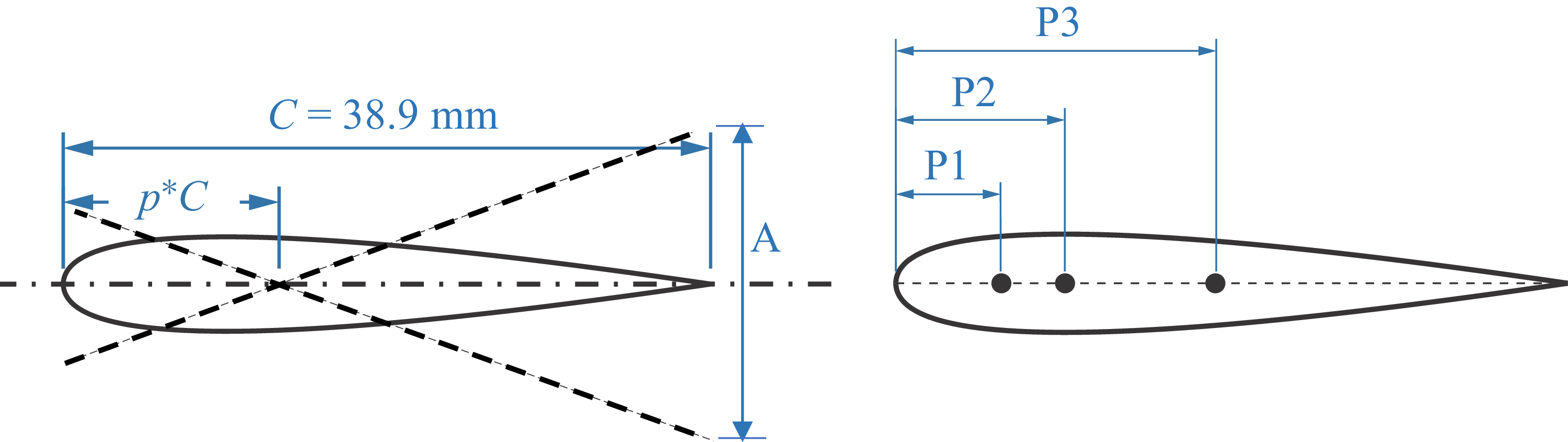
 p=0.125
 p=0.3
 p=0.48

 Us
 UTE
 Res
 ReTE=fAC/ν

 ks=πfC/Us
 UBL∗=Us/fC
 θ0
 UBL∗=π/ks
 UBL∗

 πθ02k2/2
 p
 k→∞

 πθ02
 k

 θ1
 p=0.25C
 θ0=2∘
 θ0=2∘
 θ2,θ3
 θ4

 UBL∗

 St
 B1=((1−p)/(1−2p))
 B2=((1−p)/(1−2p)1/2)

 p=0.48

 Ref−θ0
 p−θ0

 θ2


 St−UBL∗
 θ0−Ref
 St
 UBL∗

 Open access

