1. Introduction
In classical fluid mechanics, it is usually accepted that when a fluid flows past a stationary solid substrate, the tangential velocity at the wall vanishes, i.e. it satisfies the no-slip condition. This behaviour arises from the strong intermolecular forces between the fluid and solid surface (Richardson Reference Richardson1973). However, for molecularly smooth, non-wetting or partially wetting surfaces, the fluid–fluid interactions dominate over the fluid–solid interactions (Thompson & Troian Reference Thompson and Troian1997; Barrat & Bocquet Reference Barrat and Bocquet1999). In such cases, the hydrodynamic models achieve greater accuracy by incorporating a partial-slip boundary condition, which permits a non-zero tangential velocity at the wall, known as the slip velocity (Watanabe, Udagawa & Udagawa Reference Watanabe, Udagawa and Udagawa1999; Rothstein Reference Rothstein2010). The experimental study by Zhu & Granick (Reference Zhu and Granick2002) explored the influence of surface roughness and fluid–solid intermolecular forces on the slip velocity across various Newtonian fluids and surfaces. A widely accepted framework for modelling the slip velocity at the solid boundary, proposed by Navier (Reference Navier1822), is given as
 \begin{equation} \left ( l_x \frac {\partial u}{\partial z} + u \right )_{\textit{wall}}=0 \quad \text{and}\quad \left ( l_y \frac {\partial v}{\partial z} + v \right )_{\textit{wall}}=0, \end{equation}
where
 $u$
and
 $v$
are the tangential velocity components, and
 $z$
is the normal direction. The parameters
 $l_x$
and
 $l_y$
represent the streamwise and spanwise slip lengths, respectively.
The slip can be introduced artificially by coating the wall surface with hydrophobic materials such as dimethyldichlorosilane or silica (Watanabe et al. Reference Watanabe, Udagawa and Udagawa1999; Lauga & Stone Reference Lauga and Stone2003). These water-repellent coatings feature fine grooves or micropores that trap small air bubbles, thus creating a barrier that prevents contact between the fluid and solid surface (Barrat & Bocquet Reference Barrat and Bocquet1999). By texturing the hydrophobic surface at the nanoscale, Choi & Kim (Reference Choi and Kim2006) achieved isotropic slip lengths (i.e.
 $l_x=l_y$
) of approximately
 $20\,{\unicode{x03BC}} \text{m}$
. Similarly, Lee, Choi & Kim (Reference Lee, Choi and Kim2008) experimentally investigated the role of geometric parameters, such as pitch and gas fraction, on slip length for textured hydrophobic surfaces. They further extended their work by nano-structuring the side walls of micro-structured surfaces (Lee & Kim Reference Lee and Kim2009), resulting in the isotropic slip lengths as high as
 $400\,{\unicode{x03BC}} \text{m}$
. In contrast, the anisotropic slip length (
 $l_x \neq l_y$
) can be incurred by texturing the surface with periodic slats or grooves aligned in a specific direction (Lecoq et al. Reference Lecoq, Anthore, Cichocki, Szymczak and Feuillebois2004; Ng & Wang Reference Ng and Wang2009; Teo & Khoo Reference Teo and Khoo2009). Using the eigenfunction expansions in groove-array configurations, Ng & Wang (Reference Ng and Wang2009) reported that the ratio of longitudinal to transverse slip lengths can vary from 0.27 to 0.8.
Recent advances in imposing slip boundary conditions have garnered significant attention due to their crucial role in tailoring flow and instability behaviour in duct flows. This has motivated numerous researchers to study the hydrodynamic stability of pressure-driven duct flows with wall slip (Lauga & Cossu Reference Lauga and Cossu2005; Min & Kim Reference Min and Kim2005; Pralits, Alinovi & Bottaro Reference Pralits, Alinovi and Bottaro2017; Chai & Song Reference Chai and Song2019; Chen & Song Reference Chen and Song2021; Ceccacci et al. Reference Ceccacci, Calabretto, Thomas and Denier2022). The isotropic slip on one or both parallel plates in a channel stabilises the flow (Lauga & Cossu Reference Lauga and Cossu2005; Min & Kim Reference Min and Kim2005; Ceccacci et al. Reference Ceccacci, Calabretto, Thomas and Denier2022). In contrast, the anisotropic slip can significantly destabilise the system in channels (Pralits et al. Reference Pralits, Alinovi and Bottaro2017; Chai & Song Reference Chai and Song2019) and pipes (Chen & Song Reference Chen and Song2021). Squire’s theorem does not hold in the case of anisotropic slip, thus allowing the least stable disturbances to be two- or three-dimensional. Additionally, these studies also reveal that the destabilising impact of spanwise slip is more pronounced than that of streamwise slip.
Apart from the single-fluid layer configurations, the flow and instability characteristics in superposed fluid–porous medium (i.e. in a two-layer configuration) have also garnered significant attention due to their wide-ranging engineering applications, including the coupled surface-groundwater flows (Layton, Schieweck & Yotov Reference Layton, Schieweck and Yotov2002), water treatment plants (Herzig, Leclerc & Goff Reference Herzig, Leclerc and Goff1970), heat exchangers (Mahjoob & Vafai Reference Mahjoob and Vafai2008), oil extraction (Anbari et al. Reference Anbari, Chien, Datta, Deng, Weitz and Fan2018) and sound absorbers (Lu, Hess & Ashby Reference Lu, Hess and Ashby1999), etc. The foundational work of Chang, Chen & Straughan (Reference Chang, Chen and Straughan2006), who employed Darcy’s law to model the flow within a porous layer and analysed the linear stability characteristics under no-slip conditions, identified three distinct instability modes: porous mode, even-fluid mode and odd-fluid mode. Since then, numerous studies on the linear stability of the flow in such systems under no-slip conditions have been conducted, and their significant contributions are well documented in the recent works of Barman, Aleria & Bera (Reference Barman, Aleria and Bera2024) and Sharma, Aleria & Bera (Reference Sharma, Aleria and Bera2024) and the articles therein.
The implications of slip on the upper wall in the fluid–porous interfacial systems are particularly relevant to microelectronic devices, where the porous medium acts as a thermal conductor by effectively dissipating the heat from the system to the surroundings (Ghahremannezhad et al. Reference Ghahremannezhad, Xu, Nazari, Ahmadi and Vafai2019). In addition, the slippery channel wall ensures a significant drag reduction and noise attenuation (Lee, Choi & Kim Reference Lee, Choi and Kim2016; Niu et al. Reference Niu, Liu, Shang, Qin and Liu2022). Beyond micro-scale applications, the hydrophobic coatings are widely employed on ship hulls and submarine bodies to reduce underwater drag and resist corrosion, thereby enhancing their efficiency over large seabeds (Ferrari & Benedetti Reference Ferrari and Benedetti2015). To the best of the authors’ knowledge, the research on slip-Poiseuille flow in fluid–porous systems is currently limited to the study of Samanta (Reference Samanta2017), who investigated the impact of isotropic slip on the wall bounding the fluid layer. Unlike the stabilising effects of slip in single-fluid configurations, his study demonstrated that slip destabilises the even and odd-fluid layer modes. Furthermore, the presence of slip caused the transition from porous mode to even-fluid mode at relatively small values of fluid layer thickness. The impact of anisotropic slip on the linear stability characteristics of Poiseuille flow in a superposed fluid–porous channel is hitherto unexplored and is one of the primary objectives of the present study. Furthermore, no theoretical or experimental investigations have yet addressed the behaviour of perturbation growth beyond infinitesimal amplitude in fluid overlying a porous layer subjected to a slippery upper plate. Therefore, the present study examines the nonlinear interaction among different harmonic modes and provides insight into the transition to turbulence in such systems.
Several well-established methods, such as weakly nonlinear stability analysis using the Stuart–Landau equation (Stuart Reference Stuart1960; Stewartson & Stuart Reference Stewartson and Stuart1971; Drazin & Reid Reference Drazin and Reid2004), direct numerical simulations (Moin & Mahesh Reference Moin and Mahesh1998) and energy stability analysis (Joseph Reference Joseph2013), are widely employed to analyse the impact of finite-amplitude disturbances on the base laminar flow. In this regard, most of the research articles regarding turbulent channel flow in superposed fluid–porous systems rely on direct numerical simulation (DNS) where the non-Darcy model is used to model the flow in porous layers (Hahn, Je & Choi Reference Hahn, Je and Choi2002; Breugem, Boersma & Uittenbogaard Reference Breugem, Boersma and Uittenbogaard2006; Rosti et al. Reference Rosti, Cortelezzi and Quadrio2015, Reference Rosti, Brandt and Pinelli2018; Zhou, Huang & Xu Reference Zhou, Huang and Xu2024). Furthermore, the existing literature either focused on turbulent flow in a three-layer (porous–fluid–porous) (Hahn et al. Reference Hahn, Je and Choi2002; Rosti et al. Reference Rosti, Cortelezzi and Quadrio2015, Reference Rosti, Brandt and Pinelli2018; Zhou et al. Reference Zhou, Huang and Xu2024) or in a two-layer (fluid–porous) system (Breugem et al. Reference Breugem, Boersma and Uittenbogaard2006; Nishiyama, Kuwata & Suga Reference Nishiyama, Kuwata and Suga2020; Kuwata & Suga Reference Kuwata and Suga2024). All these studies mainly focus on the role of a fixed permeable boundary on the turbulent flow in the channel, where the fluid-to-porous depth ratio is greater than or equal to one. The influence of streamwise and spanwise slip velocities at the fluid–porous interface on the friction coefficient has also been investigated. Additionally, some researchers (Hill & Straughan Reference Hill and Straughan2009; Hill & Carr Reference Hill and Carr2010a , Reference Hill and Carrb ; McCurdy, Moore & Wang Reference McCurdy, Moore and Wang2019) have used energy stability theory to understand the transition to turbulent flow over a porous layer. However, the application of Landau theory to understand the mechanisms and conditions that trigger the transition from laminar to turbulent Poiseuille flow in the fluid overlying a porous system is limited to the studies of Aleria, Khan & Bera (Reference Aleria, Khan and Bera2024) (where the porous layer is isotropic and homogeneous) and Aleria & Bera (Reference Aleria and Bera2024) (where the porous layer is anisotropic and inhomogeneous). They have reported that, in contrast to purely fluid channels, where Poiseuille flow is subcritically unstable, the fluid overlying a porous layer may be subcritically or supercritically unstable, depending on the parameter values. As pointed out by Hof et al. (Reference Hof, Westerweel, Schneider and Eckhardt2006) and Eckhardt et al. (Reference Eckhardt, Schneider, Hof and Westerweel2007), in the subcritical bifurcation, turbulence appears suddenly when the disturbance amplitude exceeds a certain threshold. However, under supercritical bifurcation, the flow progresses through a series of secondary states before eventually transiting to turbulence. So we are curious to know whether, similar to flow through a flexible tube (Verma & Kumaran Reference Verma and Kumaran2012), turbulence of Poiseuille flow in fluid overlying the porous layer may appear suddenly or through a series of secondary states.
From the above-mentioned state of the art, it is clear that the slip condition (isotropic or anisotropic) plays a significant role in the early or late instability of the wall-bounded flows and in the transition mechanism to turbulence. However, we still have the following questions. (i) How does the anisotropic slip influence the onset of instability and the critical mode under linear stability analysis for different interface locations in the fluid–porous system? (ii) What will be its impact on the bifurcation phenomena of the above-mentioned flow? How does the impact of slip depend on the location of the interface when the depth of the porous layer is higher than the fluid layer? (iii) Can weakly nonlinear theory predict an early transition to turbulence compared with linear stability theory? If so, what factors contribute to flow instability in the subcritical regime? (iv) How does the skin-friction at the upper wall and interface change from the basic to the distorted state? These questions serve as the primary objectives of the present study, and to answer the above-raised questions, a comprehensive account of the linear and weakly nonlinear stability features of Poiseuille flow in the fluid overlying a porous medium subject to streamwise-dominant slip on the upper plate is provided. Note that the distinct instability behaviour of slip components in the streamwise and spanwise directions requires an independent analysis of these two cases (Chai & Song Reference Chai and Song2019; Chen & Song Reference Chen and Song2021). Apart from this, the anisotropic slip can be induced by texturing the surface with periodic slats or grooves aligned in a specific direction and fluids experience higher slip when flowing parallel to grooves. We shall focus primarily on the effect of streamwise slip on parallel flow under the present configuration. However, to better understand the role of slip, a brief discussion of spanwise slip, along with streamwise slip, is also provided. Thus, the present study is restricted to the case of streamwise dominant slip only.
The manuscript is organised as follows. The problem description and the basic flow of the study are outlined in § 2. The linear stability analysis, including the problem formulation, numerical methodology, data validation and the linear stability results on the impact of the streamwise slip, is presented in § 3. The weakly nonlinear stability analysis, covering the formulation of finite-amplitude equations, solution methodology and data validation, the nonlinear kinetic energy spectrum, and weakly nonlinear results related to the streamwise slip length, is depicted in § 4. The impact of other controlling parameters, which include the influence of spanwise slip, Darcy number, porosity and Beavers–Joseph on the flow instability and bifurcation behaviour, is given in § 5. Comparison with the experiments is highlighted in § 6. Finally, the summary and conclusion are drawn in § 7.
Physical and mathematical description of the flow domain.

2. Problem description and base flow
The problem under consideration involves a long horizontal channel bounded between two impermeable plates, as shown in figure 1. The channel consists of a porous layer of thickness
 $d_m$
beneath a fluid layer of thickness
 $d$
. The flow is driven by an external pressure gradient applied uniformly across the porous and fluid regions in the horizontal direction. The porous medium is isotropic and homogeneous, ensuring that the permeability,
 $k$
, is independent of position and direction. We set up the Cartesian coordinate system
 $(x,y,z)$
such that the fluid–porous interface is at
 $z=0$
. In this system,
 $x$
,
 $y$
and
 $z$
represent the respective streamwise (flow), spanwise and vertical directions. The corresponding velocity components in the fluid region are denoted by
 $u$
,
 $v$
and
 $w$
, respectively. We use analogous notation with the subscript
 $p$
in the porous region. The upper plate exhibits the anisotropic slip, characterised by the slip lengths,
 $l_x$
and
 $l_y$
, in the streamwise and spanwise directions.
The fluid is incompressible with constant density (say
 $\rho$
) and Newtonian, thus allowing the flow in the fluid domain to obey the classical Navier–Stokes equations. The value of porosity is taken as
 $\epsilon \leqslant 0.4$
. Thus, the unsteady Darcy’s law models the flow in the porous region (Straughan Reference Straughan2002; Nield & Bejan Reference Nield and Bejan2006). The dimensionless scales for length, velocity, time and pressure in the fluid domain are taken as
 $d$
,
 $U_{m}$
,
 $d/U_{m}$
and
 $\mu U_{m}/d$
, respectively. The similar scales for the quantities in porous domain are
 $d_{p}$
,
 $U_{\textit{pm}}$
,
 $d_{p}/U_{\textit{pm}}$
and
 $\mu U_{\textit{pm}}/d_{\!p}$
. Here,
 $U_{m}$
and
 $U_{\textit{pm}}$
are the maximum of base laminar velocities in the fluid and porous regions, while
 $\mu$
denotes the dynamic viscosity of fluid. Thus, the non-dimensionalised governing differential equations read as
 \begin{equation} \boldsymbol{\nabla }\boldsymbol{\cdot }\boldsymbol{v}=0, \quad \textit{Re} \left [ \frac {\partial \boldsymbol{v}}{\partial t} + ( \boldsymbol{v} \boldsymbol{\cdot }\boldsymbol{\nabla }) \boldsymbol{v} \right ] = -\boldsymbol{\nabla }\!p + {\nabla} ^2 \boldsymbol{v}, \end{equation}
in the fluid region
 $0 \leqslant z \leqslant 1$
, and
 \begin{equation} \boldsymbol{\nabla}_{\!p} \boldsymbol{\cdot }\boldsymbol{v}_{\!p}=0, \quad \frac { \textit{Re}_{\!p}}{\epsilon } \frac {\partial \boldsymbol{v}_{\!p}}{\partial t_{\!p}} = -\boldsymbol{\nabla}_{\!p} p_{\!p} + \frac {1}{\textit{Da}} \boldsymbol{v}_{\!p}, \end{equation}
in the porous region
 $-1 \leqslant z_{\!p} \leqslant 0$
. Here,
 $\boldsymbol{v}=u \hat{i}+v\! \hat{j}+w \hat{k}$
(
 $\boldsymbol{v}_{\!p}=u_{\!p} \hat{i}+v_{\!p} \hat{j}+w_{\!p} \hat{k}$
) and
 $p$
(
 $p_{\!p}$
) are the respective dimensionless velocity vector and pressure field in the fluid (porous) region. The Reynolds numbers in the fluid and porous regions are defined as
 $\textit{Re}={\rho U_m d}/{\mu }$
and
 $ \textit{Re}_{\!p}={\rho U_{\textit{pm}} d_{\!p}}/{\mu }$
, respectively. The quantity
 ${\textit{Da}}=({k}/{d_{p}^{2}})$
denotes the Darcy number. The dimensionless boundary conditions for the system (2.1) and (2.2) are as follows.
At the lower plate
 $z_{\!p}=-1$
, no penetration condition is satisfied, i.e.
 \begin{equation} w_{\!p}=0. \end{equation}
At the upper plate
 $z=1$
, the streamwise and spanwise velocity slip along with no penetration conditions hold, i.e.
 \begin{equation} L_x \frac {\partial u}{\partial z} + u=0, \quad L_y \frac {\partial v}{\partial z} + v=0, \quad w=0, \end{equation}
where the dimensionless streamwise and spanwise slip lengths are defined as
 $L_x={l_x}/{d}$
and
 $L_y={l_y}/{d}$
, respectively. The continuity of normal velocities and pressures at the interface, i.e.
 $z=z_{\!p}=0$
, gives
 \begin{equation} \textit{Re}\, w= \textit{Re}_{\!p} \hat{d} w_{\!p}, \quad \textit{Re} \, p= \textit{Re}_{\!p} \hat{d}^2 p_{p}. \end{equation}
It is noteworthy that some research works incorporate the normal stress balance condition instead of continuity of pressures (Liu, Liu & Zhao Reference Liu, Liu and Zhao2008; Sharma, Bera & Sharma Reference Sharma, Bera and Sharma2025). We have numerically verified that, under both boundary conditions, the stability characteristics remain almost the same. Thus, we have adopted the pressure continuity as the interfacial condition in this study. Additionally, the tangential slip boundary condition proposed by Beavers & Joseph (Reference Beavers and Joseph1967) is employed at the interface, i.e.
 \begin{equation} \textit{Re} \frac {\partial {u}}{\partial z} =\frac {\alpha _{_{\textit{BJ}}} \hat{d}}{\sqrt {\textit{Da}}} \big [ \textit{Re} {u} - \textit{Re}_{\!p} \hat{d} {u}_{\!p} \big ], \quad \textit{Re} \frac {\partial {v}}{\partial z} =\frac {\alpha _{_{\textit{BJ}}} \hat{d}}{\sqrt {\textit{Da}}} \big [ \textit{Re} {v} - \textit{Re}_{\!p} \hat{d} {v}_{\!p} \big ], \end{equation}
where
 $\alpha _{_{\textit{BJ}}}$
is the experimentally determined Beavers–Joseph constant. The depth ratio,
 $\hat{d}={d}/{d_{\!p}}$
, denotes the relative thickness of fluid region with respect to the same in porous region.
This article examines the instability and bifurcation characteristics of steady, unidirectional and fully developed flow in the streamwise direction. Under these flow conditions, the governing equations (2.1) and (2.2) can be represented in operator form as follows:
 \begin{equation} \mathcal{L} \left ( U_0, P_0 \right )=\frac {\text{d}^2 U_0}{\text{d} z^2}-\frac {\text{d}P_0}{\text{d} x} = 0 \end{equation}
and
 \begin{equation} \mathcal{L}^p \left ( U_{0p}, P_{0p}, Da \right )=-\frac {U_{0p}}{\textit{Da}}-\frac {\text{d}P_{0p}}{\text{d} x_{\!p}}=0, \end{equation}
subject to the boundary conditions
 \begin{equation} \textit{Re} \frac {\text{d} {U_0}}{\text{d} z} =\frac {\alpha _{_{\textit{BJ}}} \hat{d}}{\sqrt {\textit{Da}}} \big [ \textit{Re} {U_0} - \textit{Re}_{\!p} \hat{d} U_{0p} \big ] \quad \text{at} \quad z=z_{\!p}=0 \end{equation}
and
 \begin{equation} L_x \frac {\text{d} U_0}{\text{d} z}+U_0=0 \quad \text{at} \quad z=1. \end{equation}
Here,
 $U_0$
and
 $P_{0}$
(
 $U_{0p}$
and
 $P_{0p}$
) are the base state velocity and pressure, respectively, in the fluid (porous) region. The dimensionless pressure gradients in the fluid and porous regions are related as
 \begin{equation} \frac {\text{d}P_{0p}}{\text{d} x_{\!p}}=\frac { \textit{Re}}{ \textit{Re}_{\!p} \, \hat{d}^3}\frac {\text{d}P_{0}}{\text{d} x}. \end{equation}
The dimensionless base flow profiles in the fluid and porous regions are expressed as
 \begin{equation} U_0(z)=\frac {-z^{2}/2+a z+b}{a^2/2+b}: \, 0 \leqslant z \leqslant 1 \end{equation}
and
 \begin{equation} U_{0p}(z_{\!p})=1: \, -1 \leqslant z_{\!p} \leqslant 0, \end{equation}
respectively. The mathematical expressions for the constants
 $b$
and
 $a$
are
 \begin{equation} b=\frac {L_x+ \frac{\alpha _{_{\textit{BJ}}} L_x \sqrt {\textit{Da}}}{\hat{d}}+ \frac{\alpha _{_{\textit{BJ}}} \sqrt {\textit{Da}}}{\hat{d}}+ \frac{1}{2}}{\frac{\alpha _{_{\textit{BJ}}} \hat{d}}{\sqrt {\textit{Da}}}+\frac{\alpha _{_{\textit{BJ}}} L_x \hat{d}}{\sqrt {\textit{Da}}}+1} \end{equation}
and
 \begin{equation} a=\frac {\alpha _{_{\textit{BJ}}} \hat{d} b}{\sqrt {\textit{Da}}}-\frac {\alpha _{_{\textit{BJ}}} \sqrt {\textit{Da}}}{\hat{d}}, \end{equation}
respectively. An explicit relation between
 $ \textit{Re}$
and
 $ \textit{Re}_{\!p}$
is
 \begin{equation} \textit{Re}_{\!p}=\frac {\textit{Re}}{\hat{d}^3} \left ( \frac {\textit{Da}}{a^2/2+b} \right ). \end{equation}
Before proceeding to the stability analyses of the flow, a note regarding the appearance of a perfectly uniform Darcy profile inside porous layer is made. The uniform Darcy profile is a consequence of adopting Darcy’s law to model flow within a porous layer. This velocity profile inside the porous region is only possible in the low Reynolds number regime, typically when
 $\textit{Re}_k \leqslant \boldsymbol{O}(1)$
, where
 $\textit{Re}_k$
is the Reynolds number based on the square root of permeability as length scale and is given as
 $\textit{Re}_k=\textit{Re}_{\!p}\sqrt {\textit{Da}}$
(Ward Reference Ward1964; Nield & Bejan Reference Nield and Bejan2006). When
 $\textit{Re}_k \gt \boldsymbol{O}(1)$
, Darcy’s law is inappropriate as the form drag due to solid obstacles is comparable to the surface drag due to friction. Accordingly, a modification in Darcy’s law will be required. However, the maximum value of
 $\textit{Re}$
taken in the present problem is
 $25\,000$
. For the consideration of
 $\hat{d}=0.1$
,
 ${\textit{Da}}=10^{-6}$
and
 $L_x=L_y=0$
, and from (2.16),
 $\textit{Re}_{\!p}$
is calculated as
 $99.77$
and the corresponding
 $\textit{Re}_k$
is given as
 $9.977 \times 10^{-2}$
, which lies within the creeping flow limit. Therefore, modelling the flow within a porous region using Darcy’s law is appropriate.
3. Linear stability analysis
3.1. Formulation of linear stability equations
To examine the stability of base laminar state, we introduce the infinitesimal perturbations
 $({u}',{v}',{w}',{p}')$
and
 $({u}'_{\!p},{v}'_{\!p},{w}'_{\!p},{p}'_{\!p})$
onto the respective base flows
 $ ( U_0(z),0,0,P_0(x) )$
and
 $ ( U_{0p}(z_{\!p}),0,0,P_{0p}(x_{\!p}) )$
within the fluid and porous regions. Each perturbed variable is expressed via normal mode expansion as
 \begin{equation} \psi ' =\hat{\psi }(z) e^{{\text{i}[\alpha (x-c t)+ \beta y]}}: \, \, \psi =u, v, w, p, \end{equation}
and
 \begin{equation} \psi '_{p} =\hat{\psi }_{\!p} (z_{\!p}) e^{{\text{i}[\alpha _{\!p} (x_{\!p}-c_{\!p} t_{\!p})+ \beta _{\!p} y_{\!p}]}}: \, \psi _{\!p}=u_{\!p}, v_{\!p}, w_{\!p}, p_{\!p}, \end{equation}
in the fluid and porous regions, respectively. The parameters
 $\alpha \in \mathbb{R}^{+}$
and
 $\beta \in \mathbb{R}^{+} \cup \{0\}$
denote the streamwise and spanwise wavenumbers, respectively, while
 $c=c_r+\text{i} c_i$
represents the wavespeed as a complex variable. The analogous quantities in the porous region are related to the same quantities in the fluid region as
 \begin{equation} \alpha _{\!p}=\frac {\alpha }{\hat{d}} \, , \quad \beta _{\!p}=\frac {\beta }{\hat{d}} \, , \quad c_{\!p}=\frac {\textit{Re}}{ \textit{Re}_{\!p} \hat{d}} c. \end{equation}
Based on (3.1) and (3.2), the base flow is classified as stable, asymptotically stable or unstable when
 $c_i$
is negative, zero or positive, respectively. The linearised perturbed system, obtained after employing the normal mode analysis and excluding the nonlinear terms, can be written in the operator form as follows:
 \begin{align} {\mathscr{L}}_{o}(\alpha , \beta , \hat{u}, \hat{v}, \hat{w})=\text{ i} \alpha & \hat{u} + \text{i} \beta \hat{v} + \frac {\text{d} \hat{w}}{\text{d} z} =0, \end{align}
 \begin{align} {\mathscr{L}}_{x}(\alpha , \beta , c, \hat{p}, \hat{u}, \hat{w}, U_0, \textit{Re}) &= \text{ i} \alpha \hat{p} - \frac {\text{d}^2 \hat{u}}{\text{d} z^2} + \text{ i} \alpha\, \textit{Re}\, U_0 \hat{u} + (\alpha ^2+\beta ^2) \hat{u} + \textit{Re} \frac {\text{d}U_0}{\text{d}z} \hat{w} \nonumber \\ &\quad- \text{i} \alpha c\, \textit{Re}\, \hat{u}=0, \end{align}
 \begin{align} {\mathscr{L}}_{y}(\alpha , \beta , c, \hat{p}, \hat{v}, U_0, \textit{Re})&=\text{ i} \beta \hat{p} - \frac {\text{d}^2 \hat{v}}{\text{d} z^2} + \text{ i} \alpha\, \textit{Re}\, U_0 \hat{v} + (\alpha ^2+\beta ^2) \hat{v} -\text{i} \alpha c\, \textit{Re}\, \hat{v}=0, \end{align}
 \begin{align} {\mathscr{L}}_{z}(\alpha , \beta , c, \hat{p}, \hat{w}, U_0, \textit{Re})&= \frac {\text{d} \hat{p}}{\text{d} z} - \frac {\text{d}^2 \hat{w}}{\text{d} z^2} + \text{ i} \alpha\, \textit{Re}\, U_0 \hat{w} + (\alpha ^2+\beta ^2) \hat{w} -\text{i} \alpha c\, \textit{Re}\, \hat{w}=0, \end{align}
in the fluid region
 $0 \leqslant z \leqslant 1$
, and
 \begin{align} {\mathscr{L}}_{o}^{p}(\alpha _{\!p}, \beta _{\!p}, \hat{u}_{\!p}, \hat{v}_{\!p}, \hat{w}_{\!p})&=\text{i} \alpha _{\!p} \hat{u}_{\!p} + \text{i} \beta _{\!p} \hat{v}_{\!p} +\frac {\text{d} \hat{w}_{\!p}}{\text{d} z_{\!p}} =0 , \end{align}
 \begin{align} {\mathscr{L}}_{x}^{p}(\alpha _{\!p}, c_{\!p}, \hat{p}_{\!p}, \hat{u}_{\!p}, \textit{Re}_{\!p}, Da, \epsilon )&=\text{i} \alpha _{\!p} \hat{p}_{\!p} + \frac {\hat{u}_{\!p}}{\textit{Da}}- \frac {\text{i} \alpha _{\!p} c_{\!p}\, \textit{Re}_{\!p}}{\epsilon } \hat{u}_{\!p}=0, \end{align}
 \begin{align} {\mathscr{L}}_{y}^{p}(\alpha _{\!p}, \beta _{\!p}, c_{\!p}, \hat{p}_{\!p}, \hat{v}_{\!p}, \textit{Re}_{\!p}, Da, \epsilon )&=\text{i} \beta _{\!p} \hat{p}_{\!p} + \frac {\hat{v}_{\!p}}{\textit{Da}} - \frac {\text{i} \alpha _{\!p} c_{\!p}\, \textit{Re}_{\!p}}{\epsilon } \hat{v}_{\!p}=0, \end{align}
 \begin{align} {\mathscr{L}}_{z}^{p}(\alpha _{\!p}, c_{\!p}, \hat{p}_{\!p}, \hat{w}_{\!p}, \textit{Re}_{\!p}, Da, \epsilon )&= \frac {\text{d} \hat{p}_{\!p}}{\text{d} z_{\!p}} +\frac {\hat{w}_{\!p}}{\textit{Da}} - \frac {\text{i} \alpha _{\!p} c_{\!p}\, \textit{Re}_{\!p}}{\epsilon } \hat{w}_{\!p}=0, \end{align}
in the porous region
 $-1 \leqslant z_{\!p} \leqslant 0$
. The disturbed system is subjected to the following boundary conditions:
 \begin{align} \hat{w}_{\!p}=0 \quad & \text{at} \quad z_{\!p}=-1, \end{align}
 \begin{align} \hat{w}=0, \quad L_x \frac {\text{d}\hat{u}}{\text{d}z}+\hat{u}=0, \quad & L_y \frac {\text{d}\hat{v}}{\text{d}z}+\hat{v}=0 \quad \text{at} \quad z=1. \end{align}
At the interface
 $z=z_{\!p}=0$
, we have
 \begin{equation} \begin{aligned} \hat{w} & =\frac { \textit{Re}_{\!p} \hat{d}}{\textit{Re}} \hat{w}_{\!p}, \quad \hat{p}=\frac { \textit{Re}_{\!p} \hat{d}^2}{\textit{Re}} \hat{p}_{\!p}, \quad D\hat{u}=\frac {\alpha _{_{\textit{BJ}}} \hat{d}}{\sqrt {\textit{Da}}} \left ( \hat{u} -\frac { \textit{Re}_{\!p}}{\textit{Re}} \hat{d} \hat{u}_{\!p} \right ), \quad \\ D\hat{v} & =\frac {\alpha _{_{\textit{BJ}}} \hat{d}}{\sqrt {\textit{Da}}} \left (\hat{v} -\frac { \textit{Re}_{\!p}}{\textit{Re}} \hat{d} \hat{v}_{\!p}\right ). \end{aligned} \end{equation}
Overall, the flow instability is mainly controlled by seven independent parameters
 $\epsilon$
,
 $Da$
,
 $\alpha _{_{\textit{BJ}}}$
,
 $\hat{d}$
,
 $L_x$
,
 $L_y$
and
 $\textit{Re}$
. The infinitesimal disturbances imposed on the base flow are characterised by streamwise (
 $\alpha$
) and spanwise (
 $\beta$
) wavenumbers. The
 $D^2$
-Chebyshev-spectral-collocation method is used to find the instability boundary (Sharma et al. Reference Sharma, Bera and Sharma2025) and is explained as follows.
3.2. Numerical methodology and data validation
The domains of linearised disturbed system (3.4)–(3.14) are first converted into
 $[-1, 1]$
by using the linear transformations
 $\xi =2z-1$
and
 $\xi _{\!p}=-2z_{\!p}+1$
in the respective fluid and porous regions. The resulting equations are solved using the
 $D^2$
-Chebyshev-spectral-collocation method (Canuto et al. Reference Canuto, Hussaini, Quarteroni and Zang1988). The discretisation is done at
 $(N+1)$
-Gauss–Lobatto points
 \begin{equation} \xi _j=\cos {\left ( \frac {\pi j}{N} \right )}, \end{equation}
where
 $N$
is the order of Chebyshev polynomial and
 $j=0,\,1,\,2,\,\ldots ,\,N$
. The discretised system reduces to the generalised eigenvalue problem given by
 \begin{equation} \mathbb{A} \hat{X}= c\mathbb{B} \hat{X}. \end{equation}
The complex square matrices
 $\mathbb{A}$
and
 $\mathbb{B}$
are of order
 $8N+8$
. The diagonal matrix
 $c$
contains the eigenvalues associated with the eigenvectors, which are columns of the square matrix
 $\hat{X}$
. The least stable eigenvalue is calculated by extracting the diagonal entry of the matrix
 $c$
for which
 $c_i$
is maximum. The eigenvector
 $\hat{X}$
corresponding to the least stable eigenvalue
 $c$
gives the disturbance field variable components as
 $\hat{X}= [ \hat{p} \, \hat{u} \, \hat{v} \, \hat{w} \, \hat{p}_{p} \, \hat{u}_{p} \, \hat{v}_{p} \, \hat{w}_{p} ]^T$
. The multivariate function
 $\tilde {X}$
, where the tilde function is given by (3.1) and (3.2), corresponding to least stable disturbance, is called fundamental disturbance. This terminology will frequently be used in the upcoming discussions. The generalised eigenvalue problem (3.16) is solved by the QZ-algorithm in MATLAB software (Moler & Stewart Reference Moler and Stewart1973).
The numerical code developed for linear stability analysis is validated (i) by examining the independence of stability results with
 $N$
and (ii) by comparing the published results as a special case of the present results. The optimal value of
 $N$
is determined when the following criterion is satisfied:
 \begin{equation} \frac {( \textit{Re}_c)_{N+10}-( \textit{Re}_c)_{N}}{(\textit{Re})_{N}} \leqslant 10^{-5}, \end{equation}
where
 $ \textit{Re}_c$
is the critical Reynolds number. For the parameters involved in the current study, we have found consistency in the numerical results when
 $N=60$
is chosen.
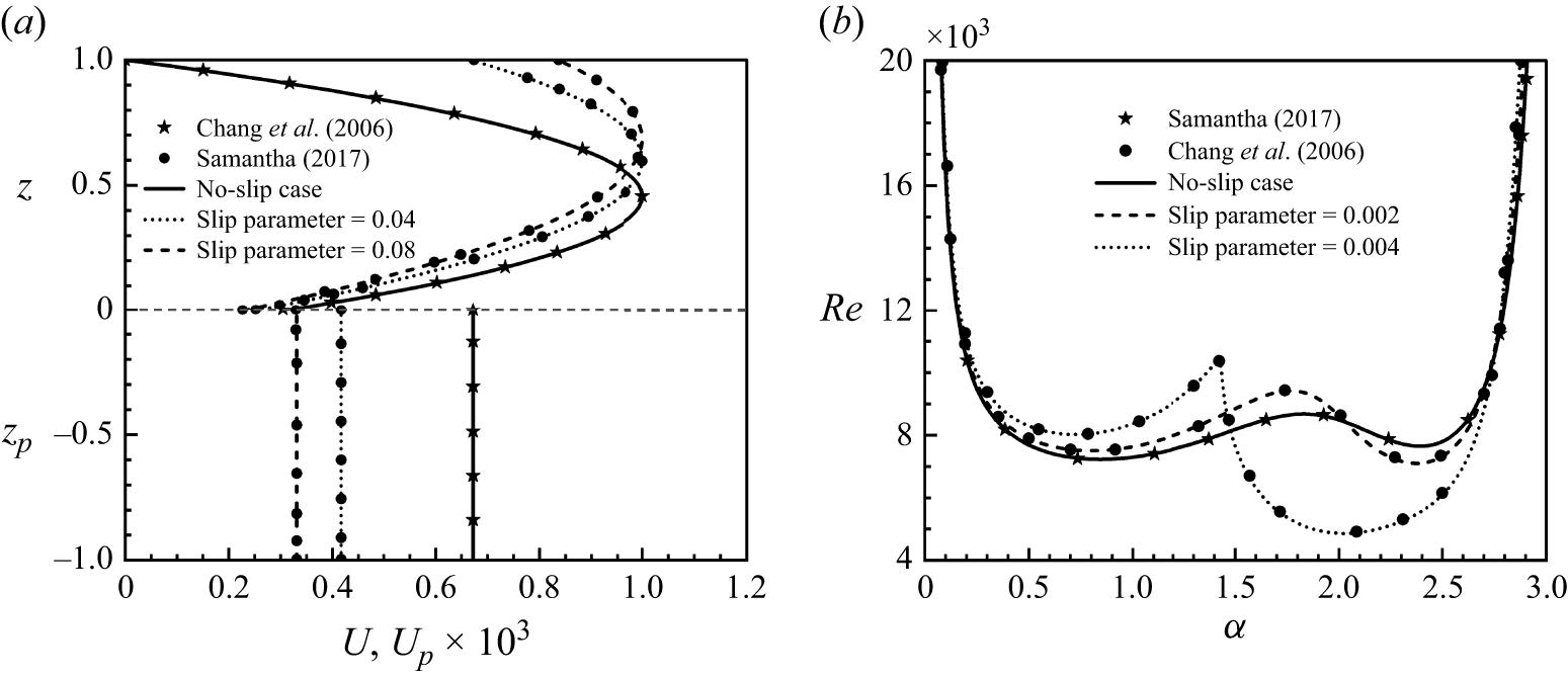
(a) Comparison of basic velocity profiles for
 $\hat{d}=0.1$
with those of Chang et al. (Reference Chang, Chen and Straughan2006), when
 $L_x=L_y=0$
and of Samanta (Reference Samanta2017) when
 $L_x=L_y\neq 0$
. (b) Comparison of neutral stability curves in the
 $(\alpha ,\textit{Re})$
-plane for
 $\hat{d}=0.11$
with those of Chang et al. (Reference Chang, Chen and Straughan2006), when
 $L_x=L_y=0$
and of Samanta (Reference Samanta2017) when
 $L_x=L_y\neq 0$
.

The current geometry can be transformed into the cases of fluid overlying porous medium in a channel, superposed fluid–porous system in a slippery channel and asymmetric slip flow in a channel to validate the linear stability results of Chang et al. (Reference Chang, Chen and Straughan2006), Samanta (Reference Samanta2017) and Ceccacci et al. (Reference Ceccacci, Calabretto, Thomas and Denier2022), respectively. Figures 2(a) and 2(b) present the basic velocity profiles for
 $\hat{d}=0.1$
and the corresponding neutral stability curves for
 $\hat{d}=0.11$
, respectively, for both no-slip and isotropic slip conditions on the upper plate. The remaining parameters are fixed at
 ${\textit{Da}}=10^{-6}$
,
 $\epsilon =0.3$
and
 $\alpha _{_{\textit{BJ}}}=0.1$
. The slip parameter used by Samanta (Reference Samanta2017) is equivalent to
 $\hat{d} L_x$
in the present formulation. Using this slip parameter, the results agree well with the published findings.
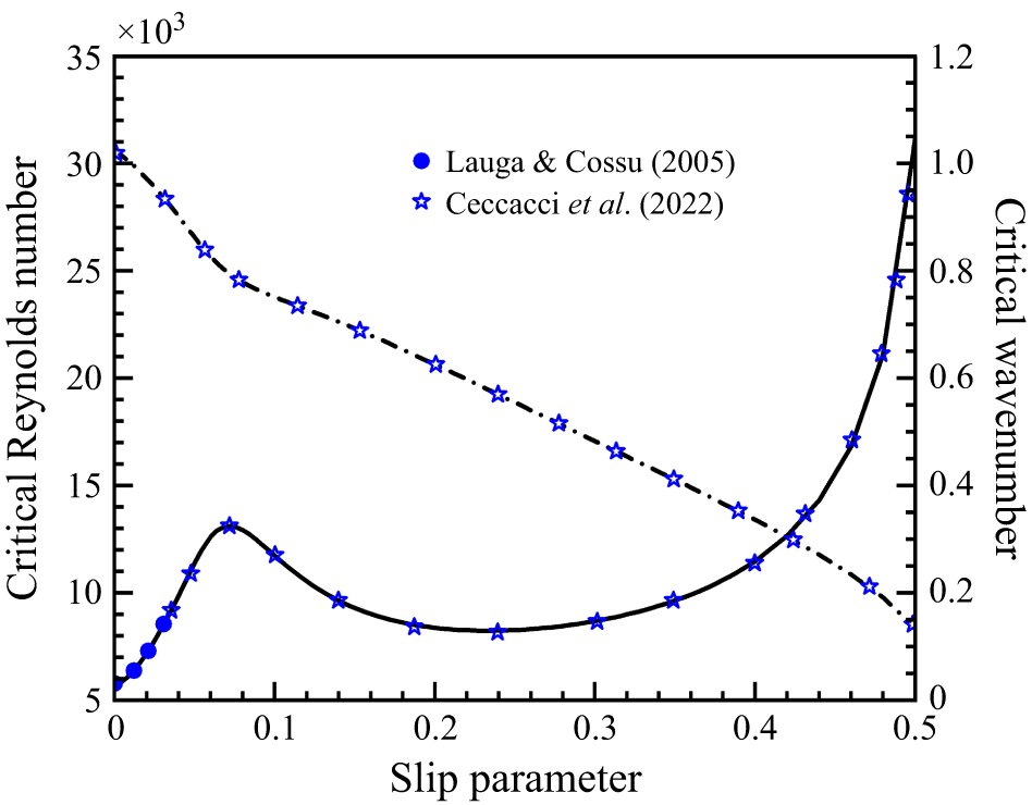
Comparison of critical Reynolds number and critical wavenumber as a function of dimensionless slip length with those of Lauga & Cossu (Reference Lauga and Cossu2005) and Ceccacci et al. (Reference Ceccacci, Calabretto, Thomas and Denier2022) for the asymmetric slip case. The dashed line shows the variation of critical
 $\alpha$
versus
 $L_x$
. The other parameters are
 ${\textit{Da}}=10^{-10}$
,
 $\hat{d}=10$
and
 $\epsilon =0.001$
.

Lauga & Cossu (Reference Lauga and Cossu2005) studied the asymmetric slip flow in a channel with slip lengths ranging from
 $0$
to
 $0.03$
. This analysis was later extended by Ceccacci et al. (Reference Ceccacci, Calabretto, Thomas and Denier2022) to accommodate larger slip values up to 0.5. The present formulation reduces to the case of asymmetric slip channel flow by setting
 ${\textit{Da}}=10^{-10}$
,
 $\hat{d}=10$
,
 $\epsilon =0.001$
,
 $L_x=L_y$
and
 $\alpha _{_{\textit{BJ}}}=0.1$
. Figure 3 shows the variation of the critical Reynolds number (indicated by the solid line) with slip length and the corresponding variation of the critical wavenumber (indicated by the dashed line). To relate the dimensionless slip length, wavenumber and critical Reynolds number used in the studies of Lauga & Cossu (Reference Lauga and Cossu2005) and Ceccacci et al. (Reference Ceccacci, Calabretto, Thomas and Denier2022), we have scaled the parameters employed here by the factors of
 $2$
,
 $1/2$
and
 ${1}/{2}\times ({L_x+1})/({2L_x+1} )^2$
, respectively. As shown in figure 3, the present numerical results under the limiting channel case match well with the published ones.
3.3. Linear stability results
This section examines the stability characteristics of Poiseuille flow in fluid overlying a porous layer with a slippery upper plate. Our numerical experiments show that for
 $\hat{d} \geqslant 0.5$
, the stability results in the fluid–porous configuration align closely with those observed in the single-fluid layer case. Parallelly, for
 $\hat{d} \lt 0.08$
, the instability characteristics of the flow remain almost independent of
 $\hat{d}$
. Thus, in this study, the range of
 $\hat{d}$
is taken as
 $[0.08, 0.5]$
. As discussed in the introduction, the maximum slip length on a superhydrophobic surface can be as considerable as
 $400 \, {\unicode{x03BC}} \text{m}$
(Lee & Kim Reference Lee and Kim2009). In the present study, the slip length parameters
 $L_x$
and
 $L_y$
are non-dimensionalised by fluid layer thickness (
 $d$
). Accordingly, if the depth of the fluid layer in the superposed fluid–porous system is 4 mm, then the maximum value of the dimensionless slip parameter will be
 $0.1$
. To cover a wide range of situations and stick to our objective, the range of
 $L_x$
is chosen as
 $[0, 0.1]$
in this study. Furthermore, for isotropic slip, i.e.
 $L_x=L_y$
, Squire’s theorem holds good (see Appendix A); however, for anisotropic slip, it does not hold. Thus, the least stable mode, i.e. critical instability point
 $(\textit{Re}_c, \alpha _c, \beta _c)$
, now onwards CIP, may be three-dimensional or two-dimensional, which our numerical experiments have also confirmed. Therefore, we have initially analysed the role of spanwise wavenumber on the mode of instability along the neutral stability curve (hereafter referred to as NSC) and its dependency on the slip condition. Subsequently, we have studied the impact of anisotropic slip conditions on the two-dimensional critical point, i.e. the least stable concerning
 $\textit{Re}$
and
 $\alpha$
only (now onwards we are defining it as 2-D critical point), and finally, the variation of CIP as a function of slip length. For analysing the NSCs and critical instability boundaries, the wavenumbers
 $\alpha$
and
 $\beta$
are varied in the range
 $[0,3]$
using discretisation steps of
 $0.001$
and
 $0.01$
, respectively. The NSCs and instability boundaries delineate the stable and unstable regimes by varying
 $\textit{Re}$
and
 $L_x$
for different
 $\hat{d}$
, while fixing the other controlling parameters. Therefore, these curves are projections of a high-dimensional stability landscape onto a reduced parameter space, which, in the two-dimensional space, reduce to single lines. To avoid numerous parametric impacts, the spanwise slip length, the Darcy number, porosity and the Beavers–Joseph coefficient are kept at
 $0$
,
 $10^{-6}$
,
 $0.3$
and
 $0.1$
, respectively. The impact of each of these parameters is analysed later in § 5.
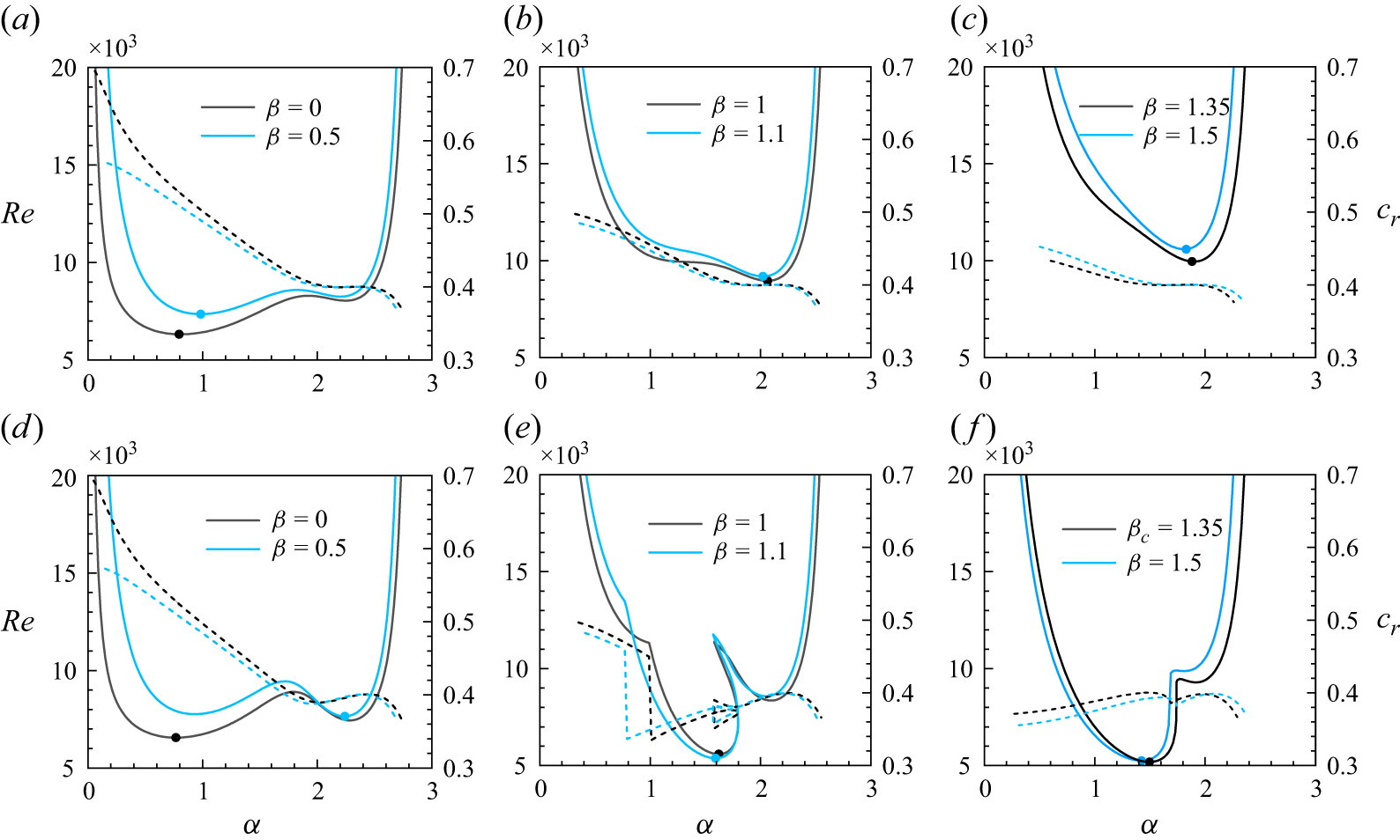
Neutral stability curves for
 ${\textit{Da}}=10^{-6}$
at
 $\hat{d}=0.1$
for different values of
 $\beta$
when (a–c)
 $L_x=0$
, and (d–f)
 $L_x = 0.02$
. The dashed curves represent the corresponding wave propagation speeds. Here,
 $\beta _c$
denotes the critical spanwise wavenumber.

3.3.1. NSC and mode of instability: role of spanwise wavenumber and slip length
The impact of spanwise wavenumber on neutral stability curves in the
 $(\alpha , \textit{Re})$
-plane for
 $\hat{d}=0.1$
is shown in figure 4(a–c) for
 $L_x=0$
and figure 4(d–f) for
 $L_x=0.02$
. Six values of
 $\beta$
, including two critical values 0 and 1.35 for
 $L_x$
equal to 0 and 0.02, respectively, are chosen. The corresponding wave propagation speed in the
 $(\alpha , c_r)$
-plane is illustrated by the dashed lines that assist in identifying the instability mode. The CIP for
 $L_x$
equal to 0 and 0.02 are
 $(6322.50, \, 0.808, \, 0)$
and
 $(5188.39, \, 1.496, \, 1.35)$
, respectively. In figures 4(a) and 4(d), each NSC shows two minima in two different lobes. The minimum in the left lobe appears at relatively small (large) values of
 $\alpha$
(
 $c_r$
) and corresponds to the porous mode of instability (Chang et al. Reference Chang, Chen and Straughan2006). The second minimum appears in the right lobe at relatively large (small) values of
 $\alpha$
(
 $c_r$
) and corresponds to the fluid mode of instability. In each NSC, the 2-D critical point is marked by a singleton bullet. The profile of wave speed shows a monotonic decrease with
 $\alpha$
in the first lobe and remains almost constant in the second lobe except in the vicinity of the end part of the second lobe, where
 $\textit{Re}$
increases rapidly and
 $c_r$
decreases on increasing the value of
 $\alpha$
. As
 $\beta$
is increased to
 $0.5$
, the instability mode at the 2-D critical point shifts from porous to fluid on changing the value
 $0$
of
 $L_x$
by
 $0.02$
. For
 $\beta = 1$
, the NSC at
 $L_x$
equal to
 $0 \, (0.02)$
possesses two (three) lobes, left and right (left, central and right), that correspond to two (three) different modes of instability, which will be analysed shortly. The minimum in the left (central) lobe dominates the instability.
In figure 4(e), the profile of wavespeed experiences a jump discontinuity as it moves from the left to the central lobe and shows a possibility of a sudden change of mode of instability. A slight increase in
 $\beta$
to
 $1.1$
results in an expansion of the unstable region in the central lobe, accompanied by a reduction in the unstable areas within the left and right lobes, and the 2-D critical point shifts downward. The left lobe vanishes completely and the minima in the central lobe become the least one for
 $\beta =1.35$
(see figure 4
f). Thus, for
 $L_x=0.02$
, the three-dimensional disturbances are least stable. Similar behaviour was also observed in the linear stability of compressible boundary layer flows with non-ideal fluids (Ren, Marxen & Pecnik Reference Ren, Marxen and Pecnik2019; Ren & Kloker Reference Ren and Kloker2022; Ren et al. Reference Ren, Wu, Mao, Wang and Kloker2025), where the appearance of three-dimensional perturbations as the least stable is possible in the transcritical and supercritical flow regimes. A further increase of
 $\beta$
to
 $1.5$
causes the 2-D critical point to rise again and reduces the right lobe’s regime, confirming the surpassing of the most unstable spanwise wavenumber. Thus, in contrast to
 $L_x=0$
, where the 2-D critical point lies in either the left or right lobe, the same for
 $L_x=0.02$
based on the value of
 $\beta$
may lie in the left, right or central lobe.
Normalised disturbed velocity contour in the wall-normal direction at 2-D critical point, for
 $L_x=0$
when (a)
 $\alpha =0.808$
,
 $\beta =0$
,
 $\textit{Re}=6322.51$
; (b)
 $\alpha = 2.063$
,
 $\beta =0.5$
,
 $\textit{Re}=8960.87$
; (c)
 $\alpha =1.90$
,
 $\beta =1.35$
,
 $\textit{Re}=9951.38$
; and for
 $L_x=0.02$
when (d)
 $\alpha =0.767$
,
 $\beta =0$
,
 $\textit{Re}=6559.38$
; (e)
 $\alpha =2.241$
,
 $\beta =0.5$
,
 $\textit{Re}=7650.00$
; ( f)
 $\alpha =1.496$
,
 $\beta =1.35$
,
 $\textit{Re}=5188.38$
.

The disturbance velocity contour plots are used to explicitly understand the mode of instability in different lobes. For this, three 2-D critical points for
 $L_x=0$
(
 $L_x=0.02$
) corresponding to
 $\beta =0$
,
 $0.5$
and
 $1.35$
are chosen. The flow patterns for the normalised disturbed velocities (
 $u_{\!p}$
and
 $u$
) in the
 $xz$
-plane for one wave period (i.e.
 $x \in [0,2\pi /\alpha ]$
) are displayed in figure 5(a–c) (figure 5
d–f) at the respective above-mentioned three points. As shown in figures 5(a) and 5(d), when the instability dominates in the left lobe, the disturbance initiates in the fluid region and penetrates through the interface into the porous region. This results in an advective flow inside the porous layer, which is mainly responsible for the onset of instability. In this case, the instability mode is defined as the porous mode (PM) of instability. In figures 5(b), 5(c), 5(e) and 5( f), the flow patterns are mostly confined to the fluid region. In figures 5(b), 5(c) and 5(e), when the instability lies in the right lobe, the contours are tilted, and there is a limited penetration of disturbance inside the porous medium. However, when the instability lies in the central lobe, the contours exhibit square-like patterns in figure 5( f) and have no penetration inside the porous medium. The pattern of eigenfunctions corresponding to figures 5(b), 5(c), 5(e) and 5( f) reveals the anti-symmetry and symmetry about
 $z=0.5$
, respectively. Thus, following Chang et al. (Reference Chang, Chen and Straughan2006, Reference Chang, Chen and Chang2017) and Sharma et al. (Reference Sharma, Aleria and Bera2024), the modes of instabilities in the former and later cases are defined as odd-fluid mode (OFM) and even-fluid mode (EFM), respectively. The mode of instability in the first and second lobes in figures 4(a), 4(b), 4(d) (figure 4
f) is also checked and found as PM and OFM (EFM and OFM), respectively. However, the same in the left, central and right lobes in figure 4(e) are identified as PM, EFM and OFM, respectively. It has also been checked that a jump in wave speed profile in figure 4(e) leads to a sudden change of mode of instability from porous to even-fluid.
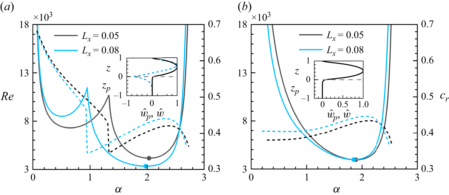
Neutral stability curves for
 ${\textit{Da}}=10^{-6}$
at
 $\hat{d}=0.1$
: (a)
 $\beta =0$
, (b)
 $\beta =0.98$
. The dashed curves represent the corresponding wave propagation speeds. The insets in panels (a) and (b) represent the normalised disturbed velocity profile at
 $(\alpha , \beta , \textit{Re})= (0.65, 0, 7311.84)$
(dashed line),
 $(\alpha , \beta , \textit{Re})= (1.972, \,0, \, 3334.90)$
(solid line) and
 $(\alpha , \beta , \textit{Re})= (1.889, \,0.98, \, 3950.86)$
(solid line) for
 $L_x=0.05$
.

So, from the above analysis, we can see that for non-zero slip length, depending on the value of
 $\beta$
, the mode of instability along the NSC may be of PM, OFM or EFM. The PM and OFM vanish for relatively higher values of
 $\beta$
. To check whether the mode of instability for
 $\beta$
equal to 0 or close to 1 can be free from OFM for some higher values of
 $L_x$
or not, the NSC is also plotted for two different values 0.05 and 0.08 of
 $L_x$
at 0 and 0.98 of
 $\beta$
in figures 6(a) and 6(b), respectively. Note that the CIP for
 $L_x$
equal to 0.05 and 0.08 are
 $(1.889, \, 0.98, \, 3950.86)$
and
 $(1.972, \, 0, \, 3334.90)$
, respectively. From figure 6(a), it can be seen that the NSC exhibits bimodal characteristics and the wave speed experiences a sudden change upon shifting from one lobe to another. Here, it has also been checked that along the NSC, the mode of instability changes from porous to even-fluid (see the inset in figure 6
a). However, the inset in figure 6(b) shows an even symmetry of the normalised disturbed velocity profile concerning
 $z=0.5$
. Thus, the unimodal behaviour of NSCs for
 $\beta =0.98$
demonstrates the even-fluid mode of instability.
3.3.2. Effect of slip length on 2-D critical point as a function of
 $\beta$
for different values of
$\hat{d}$


Thus far, the instability characteristics along the NSCs in figures 4 and 6 were investigated for a fixed depth ratio
 $\hat{d}=0.1$
and four discrete values of
 $L_x$
. For
 $L_x$
equal to zero, the instability mode at CIP is porous; for the other three values, it is even-fluid. The critical value of
 $\textit{Re}$
at
 $L_x=0$
is higher than that at
 $L_x = 0.08$
. Considering four values (0, 0.02, 0.05, 0.08) of
 $L_x$
, we can see that the least stable disturbances change from two-dimensional to three-dimensional and then again to two-dimensional. The change of dimension of the least stable disturbances on changing the value of slip length makes us curious to know that, under such slip conditions, how do the same changes on varying the values of
 $\hat{d}$
? What will be the role of
 $\beta$
on it? To answer these queries and shed more light on the mechanism of instability at each 2-D critical point, figures 7(a–c) and 7(d–f) are plotted for
 $L_x$
equal to
 $0.02$
and
 $0.05$
, respectively. The dot point in each curve represents the location of
 $\beta _c$
.
Variation of 2-D critical parameters
 $\textit{Re}$
,
 $\alpha$
and
 $c_r$
with
 $\beta$
for different values of
 $\hat{d}$
, when (a,b,c)
 $L_x=0.02$
, and (d,e, f)
 $L_x=0.05$
. The dot represents the location of
 $\beta _c$
for the critical instability point.

In figure 7(a–c), when
 $\hat{d}$
is equal to 0.08 and 0.5, the two-dimensional disturbances dominate the flow instability, i.e. CIP is two-dimensional; however, for other values of
 $\hat{d}$
, it is three-dimensional. To identify the instability mode at any 2-D critical point, we shall follow the definition of the mode of instability as a function of
 $c_r$
and by looking at the nature of the corresponding eigenfunction. As discussed in the previous subsection along the NSC, for a porous (even-fluid) mode of instability, the value of
 $c_r$
is high (low) and the
 $c_r$
profile experiences a jump whenever the PM instability is changed into EFM. When the value of
 $c_r$
continuously decreases and shows a constant nature for a small sub-interval of
 $\alpha$
and then decreases further, it indicates the change of instability from PM to OFM. However, when EFM is changed into OFM, it introduces either a jump or a cusp point on the profile of
 $c_r$
. It has been checked that a similar characteristic of the
 $c_r$
profile as a function of
 $\beta$
can be correlated for identifying the mode of instability for any 2-D critical point.
Due to the relatively small (large) value of
 $\alpha _c$
as well as the large (small) value of
 $c_r$
at
 $\hat{d}$
equal to 0.08 (0.5), the mode of instability at the critical instability point (CIP) is porous (even-fluid), which is also confirmed by checking the nature of corresponding eigen-function in figure 21 (see Appendix B). For
 $L_x = 0.02$
, we have already seen that the mode of instability at CIP is EFM for
 $\hat{d}=0.1$
, which is also the mode of instability at CIP for other depth ratios, except for
 $\hat{d}=0.08$
(see figure 21). In contrast, for
 $L_x=0.05$
, the mode of instability at CIP for all considered values of
 $\hat{d}$
is EFM. Furthermore, the instability boundary curve at
 $L_x = 0.02$
,
 $\hat{d}=0.08$
have two lobes. In the first lobe up to
 $\beta =1.45$
, the value
 $\alpha$
(
 $c_r$
) increases (decreases) smoothly, and then jumps to a large value and remains almost constant (jumps to a small value and remains practically constant). The second lobe starts with a jump discontinuity, where the value of
 $\alpha$
(
 $c_r$
) increases near the discontinuity and then decreases smoothly (experiences a sudden drop and then increases). It has been checked that in the first lobe, the mode of instability is PM except in the sub-interval of
 $\beta$
in which
 $\alpha$
experiences a jump and remains almost constant, and the mode of instability is checked as OFM. In the second lobe,
 $\alpha$
(
 $c_r$
) decreases (increases) smoothly and the mode of instability of any 2-D critical point is found as EFM. For
 $\hat{d}=0.1$
, the instability modes at
 $\beta$
equal to 0 and 0.5 are checked as PM and OFM, respectively, whereas at
 $\beta$
equal to
 $1, \, 1.1, \, 1.35$
and
 $1.5$
are EFM (see figure 4
d–f). For other values of
 $\hat{d}$
, EFM prevails as the mode of instability along the entire 2-D instability boundary.
As the value,
 $0.02$
of
 $L_x$
is replaced by 0.05, only at
 $\hat{d} = 0.08$
, the 2-D instability curve in figure 7(d) has two lobes. The first lobe shows a tendency to die out when the value of
 $L_x$
is replaced by 0.05. The profiles of wavenumber as well as wave speed for
 $L_x$
equal to 0.05 show the mode of instability at any 2-D critical point in the first lobe as PM, and in the second lobe as EFM.
Effect of
 $L_x$
on (a)
 $\textit{Re}_c$
, (b)
 $\beta _c$
, (c)
 $\alpha _c$
and (d)
 $c_r$
for different values of
 $\hat{d}$
.

3.3.3. Three-dimensional critical point as a function of slip length, for different values of
$\hat{d}$

To understand the explicit role of anisotropic slip length on the CIP, the instability boundary curves in the (
 $L_x, \textit{Re}_c$
)-, (
 $L_x, \beta _c$
)-, (
 $L_x, \alpha _c$
)-planes and the corresponding wave speed profile in the (
 $L_x, c_r$
)-plane, with discretisation step
 $0.001$
for
 $L_x$
, are plotted in figure 8(a–d), respectively, for different values of
 $\hat{d}$
. It can be seen from figure 8(a–c) that each instability boundary curve can be split into three components. In the first component, i.e. in the vicinity of the no-slip condition, the least stable disturbance is two-dimensional, whereas in the second and third components, the least stable disturbances for each CIP are three-dimensional and two-dimensional, respectively. It can also be seen that the variation of
 $\textit{Re}_c$
with
 $L_x$
in the first component is primarily influenced by the critical mode of instability of CIP under the no-slip conditions. For
 $\hat{d} \lt 0.12$
, the PM instability dominates, while for
 $\hat{d} \gt 0.12$
, the EFM mainly triggers the instability under the no-slip case (see figure 8
d). Under the same conditions, for
 $\hat{d} = 0.12$
, the OFM emerges as the most unstable mode, which is confirmed by looking at the structure of the corresponding eigenfunction. In general, when PM or EFM dominates the instability under the no-slip condition, figure 8(a) indicates that a slight increase in
 $L_x$
from the no-slip case enhances the stability of the flow. In contrast, the same destabilises the flow when the OFM dominates the flow instability, as shown in the inset of figure 8(a). Based on the corresponding
 $c_r$
profile, we see that the instability mode in the second and third components is EFM. Furthermore, the length of the subinterval of
 $L_x$
in the second component decreases on increasing the depth of the fluid layer, i.e. by increasing the value of
 $\hat{d}$
, which is also expected since the least stable disturbances in the limiting-channel plane Poiseuille flow are two-dimensional.
4. Weakly nonlinear stability analysis
The linear stability analysis can predict the impact of infinitesimally small perturbations on the base flow. However, even in the subcritical Reynolds number regime, the non-normal nature of the linearised disturbance system causes infinitesimal perturbations to grow transiently before ultimately decaying (Schmid & Henningson Reference Schmid and Henningson2001). In some cases, the transient growth can be strong enough to cause up to a hundred times increase in the initial energy of a perturbation. In such cases, the size of the initial perturbation no longer remains infinitesimal and the nonlinear effects prevail (Grossmann Reference Grossmann2000). The disturbance reaches a magnitude at which Reynolds stress alters the basic flow and linear theory cannot adequately describe the flow instability. Consequently, a nonlinear stability analysis is necessary to account for the effects of finite-amplitude perturbations on the laminar base flow. As discussed in the introduction, in this article, we will follow the cubic-Landau analysis developed by Stuart (Reference Stuart1960) and Watson (Reference Watson1960).
4.1. Formulation of finite-amplitude equations
We derive the cubic Landau equation by using the finite-amplitude expansion method (Yao & Rogers Reference Yao and Rogers1992; Sharma, Khandelwal & Bera Reference Sharma, Khandelwal and Bera2018; Aleria et al. Reference Aleria, Khan and Bera2024). The field variables are first separated into Fourier components of the disturbance wave predicted by linear theory. Each harmonic component is then expanded in terms of the parameter
 $c_i$
and an amplitude function
 $B$
. Thus, the Fourier expansion of field variables in the fluid and porous regions is given by
 \begin{align} \phi (x,y,z,t)&=\varPhi (z,\tau ) E^0 + \phi _1 (z,\tau ) E^1 + \phi _2 (z, \tau ) E^2 + \cdots + \text{c.c.} \nonumber \\ &=E^0 \big [ \varPhi _0 (z) + c_i \big | B(\tau ) \big |^2 \varPhi _1 (z) + {\boldsymbol{O}} \big (c_i^2\big ) \big ] \nonumber \\ &+E^1 \big [ c_i^{{1}/{2}} B \phi _{10} + c_i^{{3}/{2}} B | B |^2 \phi _{11} + {\boldsymbol{O}} \big ( c_i^{{5}/{2}} \big ) \big ] \nonumber \\ &+E^2 \big [ c_i B^2 \phi _{20} + {\boldsymbol{O}} \big ( c_i^2 \big ) \big ] + \cdots + \text{c.c.}; \, \phi =p,u,v,w, \quad\text{and} \end{align}
 \begin{align} \phi _{\!p}(x_{\!p},y_{\!p},z_{\!p},t_{\!p})&=\varPhi _{p}(z_{p},\tau _{p}) E_{p}^0 + \phi _{1p} (z_{\!p},\tau _{\!p}) E_{p}^{1} + \phi _{2p} (z_{p}, \tau _{p}) E_{p}^2 + \cdots + \text{c.c.} \nonumber \\ &=E_{p}^0 \big [ \varPhi _{0p} (z_{\!p}) + c_{ip} \big | B_{\!p}(\tau ) \big |^2 \varPhi _{1p} (z_{\!p}) + {\boldsymbol{O}} \big ( c_{ip}^2 \big ) \big ] \nonumber \\ &+E_{p}^1 \big [ c_{ip}^{{1}/{2}} B_{p} \phi _{10p} + c_{ip}^{{3}/{2}} B_{p} \big | B_{p} \big |^2 \phi _{11p} + {\boldsymbol{O}} \big ( c_{ip}^{{5}/{2}} \big ) \big ] \nonumber \\ &+E_{p}^2 \big [ c_{ip} B_{p}^2 \phi _{20p} + {\boldsymbol{O}} \big (c_{ip}^2\big ) \big ] + \cdots + \text{c.c.}; \quad \phi _{\!p}=p_{\!p},u_{\!p},v_{\!p},w_{\!p}, \end{align}
respectively. Here,
 $E=e^{\text{i} [ \alpha ( x-c t )+ \beta y ]}$
,
 $E_{\!p}=e^{\text{i} [\alpha _{\!p} ( x_{\!p}-c_{\!p} t_{\!p} )+ \beta _{\!p} y_{\!p} ]}$
and
 $\text{c.c.}$
denotes the complex conjugate. The amplitude function
 $B$
in the fluid region is a function of the time scale
 $\tau =c_i t$
. The multiple time scale approach is used to derive an evolutionary equation for a slowly varying amplitude. In the Fourier expansion, two types of time scales are used: (i) fast time scale (
 $t$
) and (ii) slow time scale (
 $\tau$
), to know the nonlinear impacts of disturbance in the flow. The fast time scale corresponds to the exponential growth of the infinitesimal disturbance. When the perturbation grows to a finite amplitude, the nonlinear effects become vital. In this regard, the slow time scale
 $\tau$
is used in determining the temporal behaviour of the disturbance. The time derivative due to the use of multiple time scales modifies as
 \begin{equation} \frac {\partial }{\partial t} \rightarrow \frac {\partial }{\partial t} + c_i \frac {\partial }{\partial \tau }. \end{equation}
The amplitude function and slow time scale
 $B_{\!p}$
and
 $\tau _{p}$
in the porous region are related to the same in fluid region as
 \begin{equation} B_{\!p}=\frac { \textit{Re}_{\!p}^{1/2} \, \hat{d}^{1/2}}{ \textit{Re}^{1/2}} B, \quad \tau _{p}=\hat{d} \tau. \end{equation}
4.1.1. Equations for different harmonics
After substituting the Fourier expansions (4.1)–(4.2) into the governing equations (2.1)–(2.2) and separating the harmonic components, the equations for different harmonics are given as follows:
 $E^0$
-harmonic equations:
 \begin{align} \mathcal{L}\! \left ( U_0, P_0 \right ) + c_i | B |^2 \left ( \mathcal{L}\! \left ( U_1, P_1 \right ) - \textit{Re} \frac {\text{d}}{\text{d}z} \left (u_{10} \tilde {w}_{10}+\tilde {u}_{10} w_{10} \right )\right ) & = {O} \big(c_i^2 \big), \end{align}
 \begin{align} \mathcal{L}^p\! \left ( U_{0p}, P_{0p}, Da \right )+c_{ip} |B_{\!p}|^2 \mathcal{L}^p\! \left ( U_{1p}, P_{1p}, Da \right ) & = {O} \big(c_{ip}^{2} \big). \end{align}
 $E^1$
-harmonic equations:
 \begin{align} & c_{i}^{{1}/{2}} B {\mathscr{L}}_{o}(\alpha , \beta , u_{10}, v_{10}, w_{10}) + c_{i}^{{3}/{2}} | B |^2 B {\mathscr{L}}_{o}(\alpha , \beta , u_{11}, v_{11}, w_{11})={O} \big (c_{i}^{{5}/{2}}\big ), \end{align}
 \begin{align} & c_{i}^{{1}/{2}} B {\mathscr{L}}_{x}(\alpha , \beta , c, p_{10}, u_{10}, w_{10}, U_{0}, \textit{Re})+ c_{i}^{{3}/{2}} | B |^2 B {\mathscr{L}}_{x}(\alpha , \beta , c, p_{11}, u_{11}, w_{11}, U_{0}, \textit{Re}) \nonumber \\ &\qquad +c_i^{{3}/{2}} \left [ \textit{Re} \frac {\text{d}B}{\text{d}\tau } u_{10} - \alpha B \textit{Re} u_{10} -B | B |^2 \mathcal{G}_x \right ]={O} \big (c_{i}^{{5}/{2}}\big ), \end{align}
 \begin{align} & c_{i}^{{1}/{2}} B {\mathscr{L}}_{y}(\alpha , \beta , p_{10}, v_{10}, U_{0}, \textit{Re})+ c_{i}^{{3}/{2}} | B |^2 B {\mathscr{L}}_{y}(\alpha , \beta , p_{11}, v_{11}, U_{0}, \textit{Re}) \nonumber \\ &\qquad +c_i^{{3}/{2}} \left [ \textit{Re} \frac {\text{d}B}{\text{d}\tau } v_{10} - \alpha B \textit{Re} v_{10} -B | B |^2 \mathcal{G}_y \right ]={O} \big (c_{i}^{{5}/{2}}\big ), \end{align}
 \begin{align} & c_{i}^{{1}/{2}} B {\mathscr{L}}_{z}(\alpha , \beta , p_{10}, w_{10}, U_{0}, \textit{Re})+ c_{i}^{{3}/{2}} | B |^2 B {\mathscr{L}}_{z}(\alpha , \beta , p_{11}, w_{11}, U_{0}, \textit{Re}) \nonumber \\ &\qquad +c_i^{{3}/{2}} \left [ \textit{Re} \frac {\text{d}B}{\text{d}\tau } w_{10} - \alpha B \textit{Re} w_{10} -B | B |^2 \mathcal{G}_z \right ]={O} \big (c_{i}^{{5}/{2}}\big ), \end{align}
 \begin{align} & c_{ip}^{{1}/{2}} B_{\!p} {\mathscr{L}}_{o}^{p}(\alpha _{\!p}, \beta _{\!p}, u_{10p}, v_{10p}, w_{10p})+ c_{ip}^{{3}/{2}} |B_{\!p}|^2 B_{\!p} {\mathscr{L}}_{o}^{p}(\alpha _{\!p}, \beta _{\!p}, u_{11p}, v_{11p}, w_{11p}) \nonumber \\ & \qquad \qquad ={{O}} \big (c_{ip}^{{5}/{2}}\big ), \end{align}
 \begin{align} & c_{ip}^{{1}/{2}} B_{\!p} {\mathscr{L}}_{x}^{p}(\alpha _{\!p}, c_{\!p}, p_{10p}, u_{10p}, \textit{Re}_{\!p}, Da, \epsilon ) \nonumber \\ & \qquad \qquad+ c_{ip}^{{3}/{2}} |B_{\!p}|^2 B_{\!p} {\mathscr{L}}_{x}^{p}(\alpha _{\!p}, c_{\!p}, p_{11p}, u_{11p}, \textit{Re}_{\!p}, Da, \epsilon ) \nonumber \\ & \qquad \qquad +\frac { \textit{Re}_{\!p} c_{ip}^{{3}/{2}}}{\epsilon } \left [\frac {\text{d}B_{\!p}}{\text{d}\tau _{\!p}} u_{10p} - \alpha _{\!p} B_{\!p} u_{10p} \right ]={{O}} \big (c_{ip}^{{5}/{2}}\big ), \end{align}
 \begin{align} & c_{ip}^{{1}/{2}} B_{\!p} {\mathscr{L}}_{y}^{p}(\alpha _{\!p}, \beta _{\!p}, c_{\!p}, p_{10p}, v_{10p}, \textit{Re}_{\!p}, Da, \epsilon ) \nonumber \\ & \qquad \qquad + c_{ip}^{{3}/{2}} B_{\!p} |B_{\!p}|^2 {\mathscr{L}}_{y}^{p}(\alpha _{\!p}, \beta _{\!p}, c_{\!p}, p_{11p}, u_{11p}, \textit{Re}_{\!p}, Da, \epsilon ) \nonumber \\ & \qquad \qquad +\frac { \textit{Re}_{\!p} c_{ip}^{{3}/{2}}}{\epsilon } \left [\frac {\text{d}B_{\!p}}{\text{d}\tau _{\!p}} v_{10p} - \alpha _{\!p} B_{\!p} v_{10p} \right ]={{O}} \big (c_{ip}^{{5}/{2}}\big ), \end{align}
 \begin{align} & c_{ip}^{{1}/{2}} B_{\!p} {\mathscr{L}}_{z}^{p}(\alpha _{\!p}, c_{\!p}, p_{10p}, u_{10p}, \textit{Re}_{\!p}, Da, \epsilon ) \nonumber \\ & \qquad \qquad +\, c_{ip}^{{3}/{2}} |B_{\!p}|^2 B_{\!p} {\mathscr{L}}_{z}^{p}(\alpha _{\!p}, c_{\!p}, p_{11p}, u_{11p}, \textit{Re}_{\!p}, Da, \epsilon ) \nonumber \\ & \qquad \qquad +\, \frac { \textit{Re}_{\!p} c_{ip}^{{3}/{2}}}{\epsilon } \left [\frac {\text{d}B_{\!p}}{\text{d}\tau _{\!p}} w_{10p} - \alpha _{\!p} B_{\!p} w_{10p} \right ] ={{O}} \big (c_{ip}^{{5}/{2}}\big ). \end{align}
 $E^2$
-harmonic equations:
 \begin{align} c_{i} B^2 & {\mathscr{L}}_{o} (2\alpha , 2\beta , u_{20}, v_{20}, w_{20}) ={{O}} \big (c_{i}^{2}\big ), \end{align}
 \begin{align} c_{i} B^2 & \Bigg [ {\mathscr{L}}_{x} (2\alpha , 2\beta , c, p_{20}, u_{20}, w_{20}, U_0, \textit{Re}) \nonumber \\ & + \textit{Re} \Bigg ( \text{i} \alpha u^{2}_{10} + \text{i} \beta u_{10} v_{10} + w_{10} \frac {\text{d} u_{10}}{\text{d} z} \Bigg ) \Bigg] ={{O}} \big (c_{i}^{2}\big ), \end{align}
 \begin{align} c_{i} B^2 & \Bigg [ {\mathscr{L}}_{y} (2\alpha , 2\beta , c, p_{20}, v_{20}, U_0, \textit{Re}) \nonumber \\ & + \textit{Re} \Bigg ( \text{i} \alpha u_{10} v_{10} + \text{i} \beta v^2_{10} + w_{10} \frac {\text{d} v_{10}}{\text{d} z} \Bigg ) \Bigg ] ={{O}} \big (c_{i}^{2}\big ), \end{align}
 \begin{align} c_{i} B^2 & \Bigg [ {\mathscr{L}}_{z} (2\alpha , 2\beta , c, p_{20}, w_{20}, U_0, \textit{Re}) \nonumber \\ & + \textit{Re} \Bigg ( \text{i} \alpha u_{10} w_{10} + \text{i} \beta v_{10} w_{10} + w_{10} \frac {\text{d} w_{10}}{\text{d} z} \Bigg ) \Bigg ] ={{O}} \big (c_{i}^{2}\big ), \end{align}
 \begin{align} c_{ip} B_{p}^2 & {\mathscr{L}}_{o}^{p} (2\alpha _{\!p}, 2\beta _{\!p}, u_{20p}, v_{20p}, w_{20p}) ={{O}} \big (c_{ip}^{2}\big ), \end{align}
 \begin{align} c_{ip} B_{p}^2 & {\mathscr{L}}_{x}^{p}(2\alpha _{\!p}, c_{\!p}, p_{20p}, u_{20p}, \textit{Re}_{\!p}, Da, \epsilon ) ={{O}} \big (c_{ip}^{2}\big ), \end{align}
 \begin{align} c_{ip} B_{p}^2 & {\mathscr{L}}_{y}^{p}(2\alpha _{\!p}, 2\beta _{\!p}, c_{\!p}, p_{20p}, v_{20p}, \textit{Re}_{\!p}, Da, \epsilon ) ={{O}} \big (c_{ip}^{2}\big ), \end{align}
 \begin{align} c_{ip} B_{p}^2 & {\mathscr{L}}_{z}^{p}(2\alpha _{\!p}, c_{\!p}, p_{20p}, w_{20p}, \textit{Re}_{\!p}, Da, \epsilon ) ={{O}} \big (c_{ip}^{2}\big ). \end{align}
The
 $\mathcal{G}$
functions defined in (4.8)–(4.10) are given by
 \begin{align} \mathcal{G}_x &=- \textit{Re} \biggl [ \text{i} \alpha \left ( u_{10} U_1 + \tilde {u}_{10} u_{20} \right ) + \text{i} \beta \left ( 2 \tilde {v}_{10} u_{20}-\tilde {u}_{10} v_{20} \right ) \biggr . \nonumber \\ & \quad \left . +\, \frac {\text{d} \tilde {u}_{10}}{\text{d} z} w_{20} + \tilde {w}_{10} \frac {\text{d} u_{20}}{\text{d} z} + w_{10} \frac {\text{d} U_1}{\text{d} z} \right ]\!, \end{align}
 \begin{align} \mathcal{G}_y & =- \textit{Re} \left [ \text{i} \alpha \left ( 2 \tilde {u}_{10} v_{20} - \tilde {v}_{10} u_{20} + v_{10} U_1 \right )+ \text{i} \beta \tilde {v}_{10} v_{20} + \frac {\text{d} \tilde {v}_{10}}{\text{d} z} w_{20} + \tilde {w}_{10} \frac {\text{d} v_{20}}{\text{d} z} \right ]\!, \end{align}
 \begin{align} \mathcal{G}_z & =- \textit{Re} \! \left [ \text{i} \alpha \left (2 \tilde {u}_{10} w_{20} - \tilde {w}_{10} u_{20} + w_{10} U_1 \right ) + \text{i} \beta \left ( 2 \tilde {v}_{10} w_{20}-\tilde {w}_{10} v_{20} \right ) + \frac {\text{d}}{\text{d} z} \left ( \tilde {w}_{10} w_{20} \right ) \! \right ]\!, \end{align}
where the symbol ‘
 $\sim$
’ in (4.5) and (4.23)–(4.25) denotes the complex conjugate. The consideration of terms above the orders of
 $c_i^{3/2}$
is not necessary for cubic Landau theory and, thus, is neglected in the present study (Khandelwal & Bera Reference Khandelwal and Bera2015; Khan, Bera & Khandelwal Reference Khan, Bera and Khandelwal2019).
The system of harmonic equations (4.5)–(4.22) is solved sequentially in the increasing powers of
 $c_i$
and
 $c_{ip}$
. Since the relations (3.3) and (4.4) indicate that the Fourier expansion coefficients in the fluid and porous region are related as
 $c^{1/2}_{i} B=c^{1/2}_{ip} B_{\!p}$
, therefore, to avoid the redundancy, the following discussion is given in terms of increasing powers of
 $c_i$
only.
At order
 $c_i^0$
, the
 $E^0$
harmonic equations are reduced to the basic state (2.7)–(2.8). Therefore, the terms
 $U_{0}$
and
 $U_{0p}$
denote the basic state velocities in fluid and porous regions, respectively. There are no contributions from
 $E^1$
and
 $E^2$
harmonics. At order
 $c_{i}^{1/2}$
, the
 $E^1$
harmonic contains the linear stability (3.4)–(3.11), and the contribution from
 $E^0$
and
 $E^2$
harmonics are zero. Therefore, the terms with ‘10’ subscript in the Fourier expansions (4.1) and (4.2) represent the solution obtained from the linear stability theory. At order
 $c_{i}^{1}$
, the equations corresponding to
 $E^0$
and
 $E^2$
harmonics contain the non-homogeneous system of linear equations to calculate the distorted mean flow and ‘20’ system, respectively. Since the non-homogeneous part on the right-hand side of these systems is known from the linear stability theory, the distorted mean function and the ‘20’ system can be easily computed. At order
 $c_{i}^{3/2}$
, the
 $E^1$
-harmonic (4.7)–(4.14) become non-homogeneous with the terms on the right-hand side containing the coefficients of
 ${\text{d}B}/{\text{d}\tau }$
,
 $B$
and
 $B | B |^2$
. These coefficients are known from the lower-order analysis. The corresponding homogeneous form of the above-mentioned system consists of the perturbed linear operator operating on the unknown functions with an ‘11’ subscript. For a non-trivial solution, the integrability condition requires that the non-homogeneous terms of
 $E^1$
-harmonic at order
 $c_i^{3/2}$
are orthogonal to the adjoint functions corresponding to the linearised disturbed system. The homogeneous adjoint equations of the linear system are given in the Appendix C. Therefore, multiplying the non-homogeneous parts in (4.7)–(4.14) with the corresponding adjoint variables
 $p^*, \, u^*, \, v^*, \, w^*, p_{\!p}^*, \, u_{\!p}^*, \, v_{\!p}^*, \, w_{\!p}^*$
, and using the normalisation condition (C17) yields the cubic Landau equation
 \begin{equation} \frac {\text{d} B}{\text{d} \tau } = \alpha B + a_1 B | B |^2, \end{equation}
where the first Landau coefficient
 $a_1$
is given by
 \begin{equation} a_1=\frac {1}{\textit{Re}} \int _{0}^{1} \big ( \mathcal{G}_x u^* + \mathcal{G}_y v^* + \mathcal{G}_z w^* \big ) \, \text{d}z . \end{equation}
Note that the Landau equation (4.26) gives a modification to the exponential growth/decay of the disturbance predicted by the linear stability analysis.
4.1.2. Physical significance of first Landau constant and amplitude function
The physical interpretation of (4.26) can be determined by the concept of equilibrium amplitude as follows.
Substituting
 $B=c_{i}^{1/2} A$
,
 $\tau =c_i t$
in the Landau equation (4.26), we get
 \begin{equation} \frac {\text{d} |A|^2}{\text{d} t}= 2 \alpha c_i |A|^2 + 2 a_{1r} |A|^4, \end{equation}
where
 $a_{1r}=\text{Real} ( a_1 )$
and
 $A$
is called physical amplitude of the disturbance wave. The stationary amplitude,
 $A_s$
of (4.28), is obtained by satisfying the stationary condition
 ${\text{d} | A |}/{\text{d} t}=0$
. This gives the possibility of three stationary amplitude solutions given by
 \begin{equation} A_s=0\, , \,\quad A_s=\pm \sqrt {-\frac {\alpha c_i}{a_{1r}}}. \end{equation}
Note that
 $A_s$
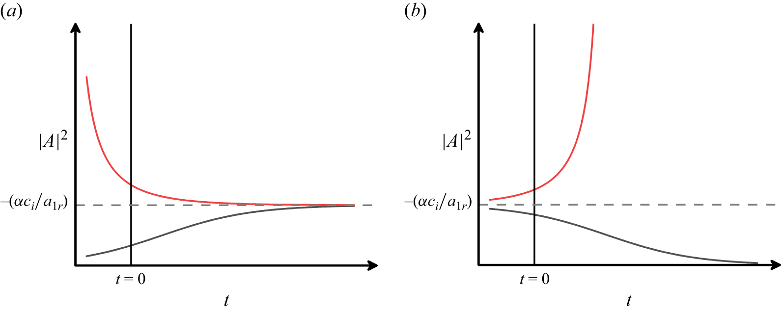
is always a positive quantity; therefore, the negative solution in (4.29) is insignificant. The nature of the other two equilibria becomes clear once the analytical solution to (4.28) is obtained, which is presented as follows (Stuart Reference Stuart1960; Khandelwal & Bera Reference Khandelwal and Bera2015):
 \begin{equation} |A|^2=\frac {A_0 c_i e^{2 \alpha c_i t}}{\left ( 1- {a_{1r}}/{\alpha } A_0 e^{2 \alpha c_i t}\right )}, \end{equation}
where
 $A_0$
is an arbitrary real constant.
Variation of physical amplitude with time in the (a) supercritical regime and (b) subcritical regime.

For
 $c_i\gt 0$
, i.e. when
 $\textit{Re} \geqslant \textit{Re}_c$
, where
 $ \textit{Re}_c$
is the critical Reynolds numbers corresponding to least stable disturbance, the solution (4.30) will be meaningful for all
 $t$
only if
 $| A |^2\gt 0$
, which is possible when
 $a_{1r}\lt 0$
. In this scenario,
 $| A |^2 \rightarrow 0$
as
 $t \rightarrow -\infty$
, and tends an equilibrium value
 $-({\alpha c_i}/{a_{1r}})$
as
 $t \rightarrow \infty$
. The phase portrait diagram for the supercritical case is shown in figure 9(a), indicating that the solutions
 $A_s=0$
and
 $A_s=\sqrt {-({\alpha c_i}/{a_{1r}})}$
correspond to unstable and stable equilibria, respectively, when
 $c_i\lt 0$
and
 $a_{1r}\gt 0$
. Since any perturbation in the supercritical regime will grow or decay to an equilibrium value of
 $\sqrt {-({\alpha c_i}/{a_{1r}})}$
, the amplitude
 $A_s$
is called the equilibrium amplitude (
 $A_e$
).
For
 $c_i\lt 0$
, i.e. when
 $ \textit{Re} \leqslant \textit{Re}_c$
, the solution (4.30) will be meaningful for all
 $t$
when
 $a_{1r}\gt 0$
. In this case,
 $| A |^2 \rightarrow -({\alpha c_i}/{a_{1r}})$
as
 $t \rightarrow -\infty$
. At some finite time
 $t_0$
, if
 $|A|^2$
is slightly less than
 $-({\alpha c_i}/{a_{1r}})$
, the amplitude of the disturbance decays to zero. However, if
 $|A(t_0)|^2 \geqslant -({\alpha c_i}/{a_{1r}})$
, the disturbance grows in magnitude. The phase portrait diagram for the subcritical case is given in figure 9(b), which shows that the solutions
 $A_s=0$
and
 $A_s=\sqrt {-({\alpha c_i}/{a_{1r}})}$
correspond to stable and unstable equilibria, respectively. Since a minimum threshold amplitude of disturbance is required to cause the flow instability, the amplitude
 $\sqrt {-({\alpha c_i}{a_{1r}})}$
in the subcritical regime is called the threshold amplitude (
 $A_t$
).
4.2. Solution methodology and data validation
The linear adjoint system (C5)–(C16) is solved by the
 $D^2$
-Chebyshev-spectral-collocation method as discussed in § 3.2. The distorted mean flow in
 $E^0$
harmonic (4.5)–(4.6) are discretised to obtain a non-homogeneous system of linear equations in
 $U_1$
and
 $U_{1p}$
. Since there is no change in the mass flux of basic flow and the mean flow obtained after the distortion (Yao & Rogers Reference Yao and Rogers1992), the distorted pressure gradient term (i.e.
 ${\text{d} P_1}/{\text{d} x}$
) can be calculated. For
 $E^2$
harmonic equations, the ‘20’ system can be obtained by solving a non-homogeneous system
 $\mathcal{A}\hat{X}_{20}=\mathcal{B}$
. Here,
 $\mathcal{A}=\mathbb{A}_1-c\mathbb{B}_1$
with
 $\mathbb{A}_1=\mathbb{A} ({\alpha \rightarrow 2\alpha , \, \beta \rightarrow 2\beta } )$
and
 $\mathbb{B}_1=\mathbb{B} ({\alpha \rightarrow 2\alpha , \, \beta \rightarrow 2\beta } )$
. Since the matrix
 $\mathcal{A}$
is non-singular, the solution of the ‘20’ system can be evaluated easily. The integral in (4.27) is solved numerically via Gauss–Chebyshev quadrature integration formula (Trefethen Reference Trefethen2000) to find the first Landau constant. A singular system of equations is encountered for the field variables with ‘11’ subscript, which is solved via singular value decomposition in the MATLAB software.
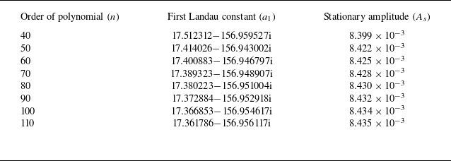
Before proceeding to weakly nonlinear results, it is necessary to validate the numerical code. It has been done in two ways. First, the response of the first Landau constant and stationary amplitude to the order of the Chebyshev polynomial was tested. Table 1 presents the impact of grid size on the first Landau constant and stationary amplitude for
 ${\textit{Da}}=10^{-6}$
,
 $\hat{d}=0.1$
,
 $\epsilon =0.3$
,
 $\alpha _{_{\textit{BJ}}}=0.1$
,
 $L_x=L_y=0$
and
 $\textit{Re}=5000$
corresponding to the linearly least disturbance wave. A convergence in the value of
 $a_{1}$
and
 $A_s$
up to 2 decimal places is found for
 $N \geqslant 100$
. Similar independency of grid size on the weakly nonlinear stability characteristics was observed for other parametric values. Therefore, the bifurcation characteristics are computed at
 $N=100$
. Second, by comparing the finite-amplitude solution for the present problem with a single-fluid layer case. The objective is achieved by choosing very small permeability and porosity values along with a high depth ratio. The linear stability theory gives the critical
 $\textit{Re}$
(based on half-channel width) as
 $5772.22$
(Orszag Reference Orszag1971). Further, Meksyn & Stuart (Reference Meksyn and Stuart1951) predicted the subcritical transition to turbulence of plane-Poiseuille flow in the range
 $2900\leqslant \textit{Re} \leqslant 5772.22$
. The present problem can be transformed into plane-Poiseuille flow in a single-fluid layer by considering
 $\epsilon =0.001$
,
 ${\textit{Da}}=10^{-10}$
,
 $\hat{d}=10$
,
 $L_x=L_y=0$
and
 $\alpha _{_{\textit{BJ}}}=0.1$
. Using these parameters, we have retrieved the critical Reynolds number at
 $5772.17$
. Upon restricting our analysis to
 ${\boldsymbol{O}}(c_i) \leqslant 10^{-3}$
, we have observed the transition to turbulence in the subcritical regime
 $2966.96 \leqslant \textit{Re} \leqslant 5772.17$
, which is in good agreement with the result of Meksyn & Stuart (Reference Meksyn and Stuart1951).
Impact of order of polynomial on the first Landau constant and the stationary amplitude corresponding to the least stable disturbances, when
 ${\textit{Da}}=10^{-6}$
,
 $\hat{d}=0.1$
,
 $\epsilon =0.3$
,
 $\alpha _{_{\textit{BJ}}}=0.1$
and
 $\textit{Re}=5000$
.

4.3. Nonlinear kinetic energy spectrum
The distortion of the basic flow by the Reynolds stress of the fundamental disturbance causes the energy transfer between the mean flow and the fundamental disturbance. To have a better understanding of the mechanism involved behind the bifurcations, an investigation of the energy balance in the superposed fluid–porous flow is required. The explicit relation for the rate of increase in the kinetic energy (KE) of the fundamental disturbance is
 \begin{align} & \frac {\partial }{\partial t} \left \langle \frac {1}{2} \left [ \overline {u_1^2}+\overline {v_1^2}+\overline {w_1^2} \right ] \right \rangle = - \left \langle \overline {u_1 w_1} \frac {\textrm{d} U}{\textrm{d} z} \right \rangle - \left \langle \overline {u_1^2 \frac {\partial u_2}{\partial x}} + \overline {u_1 v_1 \frac {\partial u_2}{\partial y}} + \overline {u_1 w_1 \frac {\partial u_2}{\partial z}} + \overline {v_1 u_1 \frac {\partial v_2}{\partial x}} \quad \quad \right . \nonumber \\ & \qquad \left . +\, \overline {v_1^2 \frac {\partial v_2}{\partial y}} + \overline {v_1 w_1 \frac {\partial v_2}{\partial z}} + \overline {w_1 u_1 \frac {\partial w_2}{\partial x}} + \overline {w_1 v_1 \frac {\partial w_2}{\partial y}} + \overline {w_1^2 \frac {\partial w_2}{\partial z}} \right \rangle \nonumber \\ & \qquad -\, \frac {1}{\textit{Re}} \left \langle \overline {\left (\frac {\partial u_1}{\partial x}\right )^2} + \overline {\left (\frac {\partial u_1}{\partial y}\right )^2} + \overline {\left (\frac {\partial u_1}{\partial z}\right )^2} + \overline {\left (\frac {\partial v_1}{\partial x}\right )^2} + \overline {\left (\frac {\partial v_1}{\partial y}\right )^2} + \overline {\left (\frac {\partial v_1}{\partial z}\right )^2} \right . \nonumber \\ & \qquad \left . +\, \overline {\left (\frac {\partial w_1}{\partial x}\right )^2} + \overline {\left (\frac {\partial w_1}{\partial y}\right )^2} + \overline {\left (\frac {\partial w_1}{\partial z}\right )^2} \right \rangle + \frac {1}{\textit{Re}} \frac {4 \pi ^2}{\alpha \beta } \big [ \overline {p_1(0) w_1(0)} \big ] \nonumber \\ & \qquad -\, \frac {2\pi ^2}{\alpha \beta } \big [ \overline {u_1^{2}(0) w_2(0)} + \overline { v_1^{2}(0) w_2(0)} +\overline {w_1^{2}(0) w_2(0)} \big ] \nonumber \\ & \qquad -\, \frac {1}{\textit{Re}} \frac {4\pi ^2}{\alpha \beta } \left [ \overline {u_1(0) \frac {\partial u_1}{\partial z} (0)} + \overline {v_1 (0) \frac {\partial v_1}{\partial z} (0)} + \overline {w_1(0) \frac {\partial w_1}{\partial z}(0)} \right ] \nonumber \\ & \qquad +\, \frac {1}{\textit{Re}} \frac {4\pi ^2}{\alpha \beta } \left [ \overline {u_1(1) \frac {\partial u_1}{\partial z} (1)} + \overline {v_1 (1) \frac {\partial v_1}{\partial z} (1)} \right ]\!, \end{align}
in the fluid region, where the bracket
 $\langle \rangle$
denotes the volume integration over
 $ [0,{2\pi }/{\alpha } ] \times [0, {2\pi }/{\beta } ]\times [0,1]$
, and
 \begin{align} \frac {\partial }{\partial t_{\!p}} \left \langle \frac { \textit{Re}_{\!p}}{2\epsilon } \left [ \overline {u_{1p}^2}+\overline {v_{1p}^2}+\overline {w_{1p}^2} \right ] \right \rangle _{\!p} = & -\!\frac {4 \pi ^2}{\alpha _{\!p} \beta _{\!p}} \big ( \overline {w_{1p}(0) p_{1p}(0)} \big )\nonumber \\ & -\!\frac {1}{\textit{Da}} \left \langle \overline {u_{1p}^2} + \overline {v_{1p}^2} + \overline {w_{1p}^2} \right \rangle _{\!p} \!, \end{align}
in the porous region, where the bracket
 $\langle \rangle _{\!p}$
denotes the volume integration over
 $ [0,{2\pi }/{\alpha _{\!p}} ] \times [0,{2\pi }/{\beta _{\!p}} ] \times [-1,0]$
. The product
 $\overline {\textit{GH}}$
, for some field variables
 $G$
and
 $H$
, implies spatial mean and is defined as
 $G\!\tilde {H}+\tilde {G} H$
. Using the Fourier expansion (4.1) and (4.2) of each field variable, and combining the fluid and porous energy components, we have
 \begin{equation} \frac {\text{d}|B|^2}{\text{d}\tau } = 2\alpha |B|^2 + \left ( P_{101} + E_{12} + P_{110} + D_{11} + K_{11} \right )\! |B|^4. \end{equation}
The comparison of (4.26) and (4.33) gives
 \begin{equation} 2 a_{1r} = P_{101} + E_{12} + P_{110} + D_{11} + K_{11}. \end{equation}
The terms in the right-hand side of (4.34) are
 \begin{align} P_{101} & =- \frac {1}{E_0} \int _{0}^{1} \left ( \overline {u_{10} w_{10}} \frac {\text{d}U_1}{\text{d}z} \right ) \text{d}z, \end{align}
 \begin{align} E_{12} & = -\frac {1}{E_0}\int _{0}^{1} \left [ \overline {u_{10}^2 \frac {\partial u_{20}}{\partial x}} + \overline {u_{10} v_{10} \frac {\partial u_{20}}{\partial y}} + \overline {u_{10} w_{10} \frac {\partial u_{20}}{\partial z}} + \overline {u_{10} v_{10} \frac {\partial v_{20}}{\partial x}}+ \overline {v_{10}^2 \frac {\partial v_{20}}{\partial y}} \right . \nonumber \\ & \quad \left . + \overline {v_{10} w_{10} \frac {\partial v_{20}}{\partial z}} + \overline {u_{10} w_{10} \frac {\partial w_{20}}{\partial x}} + \overline {v_{10} w_{10} \frac {\partial w_{20}}{\partial x}}+ \overline {w_{10}^2 \frac {\partial w_{20}}{\partial x}} \right ] \text{d}z \nonumber \\ & \quad + \frac {1}{2 E_0} \left [ \overline {u_{10}^{2}(0) w_{20}(0)} + \overline { v_{10}^{2}(0) w_{20}(0)} +\overline {w_{10}^{2}(0) w_{20}(0)} \right ]\!, \end{align}
 \begin{align} P_{110} & =-\frac {1}{E_0} \int _{0}^{1} \left ( \overline {u_{10} w_{11}}+\overline {u_{11} w_{10}} \right ) \frac {\text{d}U_0}{\text{d}z}\, \text{d}z, \end{align}
 \begin{align} D_{11} & =-\frac {2}{ \textit{Re} E_0} \int _{0}^{1} \left [ \overline {\frac {\partial u_{10}}{\partial x} \frac {\partial u_{11}}{\partial x}} + \overline {\frac {\partial u_{10}}{\partial y} \frac {\partial u_{11}}{\partial y}} +\overline {\frac {\partial u_{10}}{\partial z} \frac {\partial u_{11}}{\partial z}} +\overline {\frac {\partial v_{10}}{\partial x} \frac {\partial v_{11}}{\partial x}} +\overline {\frac {\partial v_{10}}{\partial y} \frac {\partial v_{11}}{\partial y}} \right . \nonumber \\ & \quad \left . +\overline {\frac {\partial v_{10}}{\partial z} \frac {\partial v_{11}}{\partial z}} +\overline {\frac {\partial w_{10}}{\partial x} \frac {\partial w_{11}}{\partial x}} +\overline {\frac {\partial w_{10}}{\partial y} \frac {\partial w_{11}}{\partial y}} +\overline {\frac {\partial w_{10}}{\partial z} \frac {\partial w_{11}}{\partial z}}\right ] \text{d}z \nonumber \\ & \quad +\frac {1}{ \textit{Re} E_0} \left [ \overline {u_{10} (1) \frac {\partial u_{11}}{\partial z} (1)} + \overline {v_{10}(1) \frac {\partial v_{11}}{\partial z}(1)} - \overline {u_{10}(0) \frac {\partial u_{11}}{\partial z}(0)} \right . \nonumber \\ & \quad \left . -\, \overline {v_{10} (0) \frac {\partial v_{11}}{\partial z} (0)} - \overline {w_{10} (0) \frac {\partial w_{11}}{\partial z} (0)} \right ]\!, \end{align}
 \begin{align} K_{11} & =-\frac {2 \hat{d}^3}{ \textit{Re}^3} \frac { \textit{Re}_{\!p}^2}{\textit{Da}} \frac {1}{E_0} \int _{-1}^{0} \left (\overline {u_{10p} u_{11p}}+\overline {v_{10p} v_{11p}}+\overline {w_{10p} w_{11p}}\right ) \text{d}z_{\!p}, \end{align}
where
 \begin{align} E_0=\frac {1}{2} \left [ \int _{0}^{1} \left ( \overline {u_{10}^2}+\overline {v_{10}^2}+\overline {w_{10}^2} \right ) \text{d}z + \frac {\hat{d}}{\epsilon } \left (\frac { \textit{Re}_{\!p}}{ \textit{Re}}\right )^2 \int _{-1}^{0} \left ( \overline {u_{10p}^2}+\overline {v_{10p}^2}+\overline {w_{10p}^2} \right ) \text{d}z_{\!p} \right ]\!. \end{align}
The physical interpretation of different integral terms involved in (4.34) is as follows. The term
 $P_{101}$
represents the gradient production of KE due to the interaction between the fundamental mode and distorted mean flow strain rate. Note that the energy required for the distortion of the base flow is received from the fundamental disturbance (see (4.5) and (4.6)), so the term
 $P_{101}$
is a negative definite quantity. The quantity
 $E_{12}$
denotes the transfer of energy from the fundamental mode to the second harmonic wave. The other integral terms
 $P_{110}$
,
 $D_{11}$
and
 $K_{11}$
arise due to the modification of the shape of the fundamental wave. The term
 $P_{110}$
denotes the modification of the gradient production of KE and can be positive or negative. The terms
 $D_{11}$
and
 $K_{11}$
represent the modification of energy due to the viscous dissipation rate and surface drag, respectively. The non-integral terms in (4.36) and (4.38) arise due to non-vanishing velocity at the interface and upper plate boundary. It is worth mentioning that the negative (positive) value of any component indicates in favour of stabilising (destabilising) the flow.
4.4. Weakly nonlinear results
We initiate our analysis by first examining the nonlinear interaction of different harmonics on the instability boundary curve, followed by an investigation along the neutral stability curve. Each point on these curves represents a bifurcation point (BP). The analysis is also extended to investigate the transitional characteristics away from the least stable critical point. A nonlinear KE-spectrum is used to reveal the underlying bifurcation characteristics. Furthermore, we will also compare the skin-friction coefficients of the basic and disturbed states to examine the impact of finite-amplitude perturbations on the flow dynamics. The analysis is carried out by fixing
 $L_y=0$
,
 ${\textit{Da}}=10^{-6}$
,
 $\epsilon =0.3$
and
 $\alpha _{_{\textit{BJ}}}=0.1$
.
4.4.1. Finite-amplitude behaviour along the instability boundary
In this subsection, we identify the nature of bifurcation by examining the real part of the Landau constant along the critical instability boundary with
 $L_x$
. Accordingly, the BP is the critical instability point (CIP) obtained from linear stability theory in figure 8.
Impact of
 $L_x$
on first Landau constant
 $a_{1r}$
along the BP, when (a)
 $\hat{d}=0.08, \, 0.10, \, 0.12$
and (b)
 $\hat{d}=0.15, \, 0.20, \, 0.30$
.

Figure 10 illustrates the variation of
 $a_{1r}$
with the streamwise slip length (
 $L_x$
) along the instability curve at various depth ratios. Since the growth rate
 $c_i$
is zero along the critical curve, the nature of bifurcation is defined only on the basis of the sign of
 $a_{1r}$
. Accordingly, for a positive (negative) value of
 $a_{1r}$
, the bifurcation is termed as subcritical (supercritical). Note that, in the vicinity of
 $L_x=0$
, for
 $\hat{d}=0.08, \, 0.10$
(PM) and for
 $\hat{d}=0.12$
(OFM), the negative sign of
 $a_{1r}$
indicates the supercritical bifurcation. As the streamwise slip increases, the nature of bifurcation shifts from supercritical to subcritical in the regime of
 $L_x$
, where three-dimensional disturbances dominate the instability. Consequently, for
 $\hat{d}=0.08, \, 0.10$
and
 $0.12$
,
 $a_{1r}$
changes its sign from negative to positive at
 $L_x=0.035, \, 0.014$
and
 $0.004$
, respectively. A further increment in
 $L_x$
lowers the magnitude of
 $a_{1r}$
and thus leads back to the supercritical bifurcation. When the two-dimensional disturbances again become least stable,
 $a_{1r}$
increases monotonically with
 $\hat{d}$
. On increasing
 $\hat{d}$
beyond
 $0.12$
in figure 10(b),
 $a_{1r}$
is positive and increases monotonically with
 $L_x$
near zero. When three-dimensional disturbances become linearly least stable,
 $a_{1r}$
decreases steadily with
 $L_x$
, attains a local minimum within the supercritical bifurcation regime and then increases toward the positive values. As two-dimensional disturbances regain dominance,
 $a_{1r}$
remains positive throughout, leading to a subcritical bifurcation. Overall, we observe that the range of
 $L_x$
where the subcritical bifurcation exists is found to be increasing monotonically with
 $\hat{d}$
. Since the type of bifurcation is subcritical for the limiting channel case (Stewartson & Stuart Reference Stewartson and Stuart1971; Orszag & Patera Reference Orszag and Patera1980), such a behaviour is anticipated for high values of
 $\hat{d}$
. Note that the bifurcation characteristics along the instability curve for
 $\hat{d}$
equal to 0.08, 0.1, 0.12 are similar and, at the same time, the bifurcation characteristics for
 $\hat{d}$
equal to 0.15, 0.2, 0.3 are identical. Therefore, to understand the impact of the location of the interface on the nonlinear evolution, we have considered two values, 0.1 and 0.2 of
 $\hat{d}$
, for the rest of the analysis.
Variation of nonlinear KE components with respect to
 $L_x$
along the BP, when (a)
 $\hat{d}=0.1$
and (b)
 $\hat{d}=0.2$
.

To uncover the driving mechanism behind the observed bifurcation characteristics, we employ the nonlinear kinetic energy (NKE) balance. Figures 11(a) and 11(b) illustrate the variation of different NKE components with
 $L_x$
along the instability curve for
 $\hat{d}=0.1$
and
 $0.2$
, respectively. In both figures, the sum of the components in the NKE spectra equals twice
 $a_{1r}$
, which supports the nonlinear stability results obtained in the present study under Landau theory. Furthermore, the magnitude of
 $K_{11}$
is almost negligible, indicating an insignificant change in the variation of KE via modification to the surface drag. At
 $L_x=0.014$
in figure 11(a), a drastic change in the NKE spectra is seen. Here, the magnitude of both
 $D_{11}$
and
 $P_{110}$
increases suddenly to large values and the positive sign of
 $D_{11}$
indicates a rapid decrease in the rate of dissipation of the disturbance. Apart from this, modification in viscous dissipation of disturbance kinetic energy due to a change in the shape of fundamental wave (i.e.
 $D_{11}$
) surpasses the combined negative contributions from
 $P_{101}$
,
 $P_{110}$
and
 $E_{12}$
, resulting in the subcritical bifurcation. As
 $L_x$
increases beyond
 $0.014$
, the continuous drop in the value of
 $D_{11}$
causes a monotonic decrease in
 $a_{1r}$
and results in supercritical bifurcation for
 $L_x \geqslant 0.041$
. In figure 11(b), the positive contributions of
 $P_{110}$
and
 $D_{11}$
drive the subcritical bifurcation over the range
 $L_x \in [0, 0.008]$
. When
 $0.009 \leqslant L_x \leqslant 0.027$
,
 $2a_{1r}$
decreases continuously and attains its negative minima. Note that at this point, the contribution of
 $P_{110}$
in NKE is almost balanced by
 $D_{11}$
, and thus the nature of bifurcation is decided mainly by gradient production due to interaction between fundamental mode and the distorted mean flow strain (i.e.
 $P_{101}$
). As
 $L_x$
increases further,
 $P_{110}$
becomes more favourable in shear production and takes the lion’s role in deciding the nature of bifurcation, thus causing the subcritical bifurcation. Additionally, for
 $L_x\geqslant 0.05$
, the bifurcation phenomena mainly depend upon
 $P_{110}$
, while the other components are stabilising in nature.
4.4.2. Bifurcation as a function of
$\alpha$

It is quite possible that the instability, which is supercritical (subcritical) at some wavenumber, may become subcritical (supercritical) at another wavenumber. In such situations, any potentially unstable wave may grow and interact with other modes. So, investigation of the bifurcation phenomenon along the NSC is essential. To address this objective, we have considered three different values
 $0$
,
 $0.02$
and
 $0.05$
of
 $L_x$
at
 $\hat{d}=0.1$
. The NSCs in the
 $(\alpha , \textit{Re})$
-plane and the variation of
 $a_{1r}$
along these curves are presented in figures 12(a), 12(b) and 12(c) for
 $\{L_x, \beta _c\}$
equal to
 $\{0,0 \}$
,
 $\{0.02,1.35\}$
and
 $\{0.05,0.98\}$
, respectively. The solid (dashed) curve represents the variation of
 $\textit{Re}$
(
 $a_{1r}$
) along the neutral curve with dot representing the
 $\textit{Re}_c$
(corresponding
 $a_{1r}$
). Under the no-slip condition, throughout the neutral curve, the negative value of
 $a_{1r}$
illustrates the supercritical bifurcation. Whereas, for
 $L_x=0.02$
, the subcritical bifurcation exists up to
 $\alpha \leqslant 1.94$
(that includes CIP) and beyond which the supercritical bifurcation persists. On further increment of
 $L_x$
to
 $0.05$
, supercritical bifurcation exists at CIP and shifts to subcritical for the relatively small values of wavenumber (see inset of figure 12
c). Therefore, the nature of bifurcation changes as one moves along the NSC.
Neutral stability curves for
 ${\textit{Da}}=10^{-6}$
at
 $\hat{d}=0.1$
for the critical spanwise disturbance when (a)
 $L_x=0$
, (b)
 $L_x=0.02$
, (c)
 $L_x=0.05$
. The corresponding dashed curves represent the variation of
 $a_{1r}$
along the neutral curve.

4.4.3. Finite-amplitude behaviour as a function of
$\textit{Re}$

The cubic Landau theory is valid only in the vicinity of BP and traces the evolution of finite-amplitude perturbations. However, according to Rogers, Moulic & Yao (Reference Rogers, Moulic and Yao1993), the analysis can also be extended beyond the BP in the limit as
 $c_i$
approaches zero. It has been reported that in the linearly stable regime, the results obtained by the cubic landau theory, quintic Landau theory and DNS are qualitatively as well as quantitatively the same for
 ${O}(c_i)\lt 10^{-3}$
, and only qualitatively for
 ${O}(c_i)\lt 10^{-2}$
. However, in the linearly unstable region, the prediction from cubic Landau theory, even for
 $c_i \leqslant 4 \times 10^{-2}$
, is well matched with the DNS results.
Being motivated by these observed validity limits, we now impose an upper bound on
 $c_i$
in the present analysis for examining the bifurcation characteristics away from the CIP. We have seen from our numerical experiments that in the linearly stable regime, each
 $a_{1r}$
curve experiences a sudden jump at some
 $\textit{Re}$
, where the magnitude of
 $a_{1r}$
becomes almost zero and does not change as one moves further away from the CIP. If we define the corresponding value of
 $c_i$
as
 $c_i^*$
, then it has been checked that the maximum absolute value of
 $c_i^*$
for the parameters considered in this study is of the order of
 $10^{-2}$
and the
 $a_{1r}$
curves are traced as a function of
 $\textit{Re}$
accordingly. Note that a complete picture of nonlinear saturation can be confirmed by the use of direct numerical simulation or higher order nonlinear analysis, which is beyond the scope of the present work. Hence, the following analysis will provide a qualitative characterisation of the nonlinear interaction between different harmonic modes for larger (lower) values of
 $\textit{Re}$
beyond (before) the bifurcation point.
The nonlinear characteristics are analysed as a function of
 $\textit{Re}$
in terms of a parameter,
 $\delta _{\textit{Re}}$
, defined by
 $\delta _{\textit{Re}}= ({\textit{Re}}/{\textit{Re}_c})-1$
. Accordingly,
 $\delta _{\textit{Re}}\lt 0$
signifies the linearly stable regime, while
 $\delta _{\textit{Re}}\gt 0$
indicates the linearly unstable regime. The results are shown for
 $0.1$
and
 $0.2$
of
 $\hat{d}$
. Figure 13 shows the variation of
 $a_{1r}$
and stationary amplitude (
 $A_s$
) as a function of
 $\delta _{\textit{Re}}$
for different values
 $(0, 0.01, 0.03, 0.05, 0.08)$
of
 $L_x$
. Figures 13(a) and 13(b) correspond to
 $\hat{d} = 0.1$
, while figures 13(c) and 13(d) correspond to
 $\hat{d} = 0.2$
. We see for both values of
 $\hat{d}$
in the linearly stable zone, each
 $a_{1r}$
curve experiences a point of discontinuity and the corresponding value of
 $c_i^*$
is given in table 2. It can be seen from figure 13(a) that for the no slip as well as slip with
 $L_x = 0.01$
cases, the sign of
 $a_{1r}$
is negative in the entire range of
 $\delta _{\textit{Re}}$
, indicating the existence of supercritical bifurcation in the linearly unstable regime which introduces stable supercritical branch of equilibrium amplitude (see figure 13
b). This also indicates the existence of a new laminar flow for
 $\textit{Re} \gt \textit{Re}_c$
. For all other values of
 $L_x$
, the sign of
 $a_{1r}$
changes from positive to negative on moving from the left-hand side to the right-hand side of the bifurcation point. It shows that both subcritical and supercritical bifurcations are possible. Therefore, branches of both stable supercritical equilibrium and unstable subcritical threshold amplitudes can be seen in figure 13(b). For
 $L_x$
equal to 0.05 and 0.08, an unstable subcritical (stable supercritical) branch appears away from (at) the bifurcation point. Interestingly, at
 $L_x=0.03$
, the sign of
 $a_{1r}$
is positive in the range
 $-0.386 \leqslant \delta _{\textit{Re}} \leqslant 0.243$
; consequently, the unstable branch of threshold amplitude appears in that range starting from the CIP and a stable branch of equilibrium amplitude appears in the unstable regime beyond
 $\delta _{\textit{Re}} = 0.243$
. As the location of the interface is shifted downward by changing the value 0.1 of
 $\hat{d}$
to 0.2, except for
 $L_x=0.03$
, the sign of
 $a_{1r}$
remains positive in the linearly stable regime and the threshold amplitude exists starting from the CIP (see figures 13
c and 13
d). For
 $L_x=0.03$
, the same starts from a point in the neighbourhood of CIP.
Critical point,
 $c_i^*$
and
 $\textit{Re}^*_{_{lc}}$
for different values of
 $\hat{d}$
and
 $L_x$
. The bold value represents when the BP for two-dimensional disturbances give a smaller
 $\textit{Re}^*_{_{lc}}$
as compared with the same at the CIP.

Variation of
 $a_{1r}$
and
 $A_s$
with
 $\delta _\textit{{Re}}$
for different values of
 $L_x$
, when (a,b)
 $\hat{d}=0.1$
and (c,d)
 $\hat{d}=0.20$
.

Variation of nonlinear KE components with respect to
 $\delta _{\textit{Re}}$
, when
 $\hat{d}=0.1$
for (a)
 $L_x=0$
, (b)
 $L_x=0.03$
, (c)
 $L_x=0.08$
; and when
 $\hat{d}=0.2$
for (d)
 $L_x=0$
, (e)
 $L_x=0.03$
, ( f)
 $L_x=0.08$
.

Thus, we see that the impact of slip on the finite-amplitude solution in the neighbourhood of BP is highly sensitive to the location of the interface. A nonlinear kinetic energy spectrum is used to understand the physics underlying this sensitivity characteristic. For this, we have chosen three values 0, 0.03, 0.08 of
 $L_x$
for both values 0.1 and 0.2 of
 $\hat{d}$
in figures 14(a–c) and 14(d–f), respectively. As seen in § 3.3.3, the least stable mode at
 $L_x$
equal to 0, 0.03, 0.08 are 2-D, 3-D and 2-D, respectively. In figure 14(a), when no slip condition is used, except for
 $D_{11}$
and
 $K_{11}$
, all other terms in the NKE spectrum are negative and
 $P_{101}$
is most dominating. Thus, even though
 $D_{11}$
and
 $K_{11}$
are not in favour of dissipating the disturbance, the energy released by the fundamental disturbance to distort the mean flow through
 $P_{101}$
is so prominent that the overall sum is negative and shows supercritical bifurcation in the regime of
 $\delta _{\textit{Re}}$
. For
 $L_x$
equal to
 $0.03$
,
 $P_{110}$
(
 $D_{11}$
) becomes the most stabilising (destabilising) factor in the entire regime and its magnitude increases as one moves to the right-hand side of BP (see figure 14
b). The nature of subcritical or supercritical bifurcation depends on whether a decrease in the rate of dissipation of disturbance dominates over the strong unwillingness in shear production of
 $P_{110}$
or vice versa. In the case of
 $L_x$
equal to 0.08 in figure 14(c), the nature of
 $P_{110}$
(
 $D_{11}$
) is reversed. Consequently, subcritical phenomena are observed away from the BP, whereas supercritical phenomena are seen starting from the BP. In contrast, at
 $\hat{d} = 0.2$
,
 $P_{110}$
is positive and increases monotonically in entire permissible range of
 $\delta _{\textit{Re}}$
for
 $L_x$
equal to
 $0$
and
 $0.08$
. Furthermore, the destabilising nature of
 $P_{110}$
also increases as the interface shifts downward. For
 $L_x=0.03$
in figure 14(e),
 $P_{110}$
and
 $D_{11}$
are decreasing in nature. Consequently, the nature of bifurcation as a function of
 $\delta _{\textit{Re}}$
resembles that of the case of
 $L_x=0.08$
when
 $\hat{d}=0.1$
. Overall, we observe that the characteristics of
 $D_{11}$
and
 $P_{110}$
decide the nature of the bifurcation. It has also been checked through our numerical experiments that as we further increase the value of
 $\hat{d}$
, the contribution of
 $P_{110}$
becomes increasingly more prominent and the nature of bifurcation remains subcritical, irrespective of the value of slip length.
Before discussing the role of finite-amplitude evolution on physical quantities, such as skin-friction, in the next subsection, an important note is made regarding the existence of a lower critical point. According to Landau’s suggestion, a lower critical point may exist in the subcritical regime. Note that the lower critical point is a threshold value of
 $\delta _{\textit{Re}}$
at which the unstable branch turns into a stable branch, which is the saddle node point, and below it, the bifurcated solution does not exist. To find such a point, one has to rely either on the DNS or higher-order quintic-Landau theory. The way the present analysis is made, the quintic Landau equation will have three stationary solutions, out of which two are stable and one is unstable. The point where the non-zero stable and unstable branches meet is called a saddle node point, and the corresponding
 $\delta _{\textit{Re}}$
gives the lower critical
 $\textit{Re}$
. The analysis based on the fifth-order Landau equation is beyond the scope of the present study. However, by the way
 $a_{1r}$
changes as a function of
 $\textit{Re}$
in the present study, it is clear that the lower critical value of
 $\textit{Re}$
cannot be smaller than
 $\textit{Re}$
calculated at
 $c_i^*$
, say
 $\textit{Re}_{lc}^*$
. Thus,
 $\textit{Re}_{lc}^*$
is defined as the probable lower critical corresponding to
 $\textit{Re}_c$
. The critical points,
 $c_i^*$
, and the corresponding
 $\textit{Re}_{lc}^*$
for different set values of
 $(\hat{d}, L_x)$
are illustrated in table 2. Interestingly, for
 $\hat{d}=0.2$
and
 $L_x = 0.01$
, it has been found that although the critical
 $\textit{Re}$
under three-dimensional disturbance is smaller than the same under two-dimensional disturbance,
 $\textit{Re}_{lc}^*$
obtained under two-dimensional disturbance is lower than the same obtained under three-dimensional disturbance (see the bold entry in table 2).
Overall, the weakly nonlinear stability analysis reveals a significant relationship between the critical mode of instability and the nature of bifurcation. The PM and OFM are always characterised by the supercritical bifurcation. However, for the EFM, two scenarios are possible: (i) dual existence of subcritical and supercritical bifurcation; or (ii) only subcritical bifurcation, depending upon the set of parameters involved. The presence of a lower critical point in the subcritical regime indicates an early onset of instability in the flow.
4.4.4. Variation of skin-friction coefficient
The transition from laminar to turbulent is always accompanied by a change in the skin-friction coefficient. Various experimental studies available in the literature have been performed to calculate the critical value of controlling parameters, such as Reynolds number, at which a change in friction drag occurs. In this regard, we now analyse the variation of the skin-friction coefficient for the basic and distorted state under the impact of finite-amplitude disturbances. The skin-friction coefficients at the upper wall and the interface are given by (Sharma et al. Reference Sharma, Khandelwal and Bera2018)
 \begin{equation} C_{w}=-\frac {2}{\textit{Re}} \left .\frac {\text{d}U}{\text{d}z}\right |_{z=1}, \quad C_{i}=\frac {2}{\textit{Re}} \left .\frac {\text{d}U}{\text{d}z}\right |_{z=0}, \end{equation}
respectively. The velocity function
 $U$
for the distorted state is determined at the stationary amplitude, i.e.
 $U_0+ A_{s}^2 U_1$
. Figure 15 illustrates the impact of streamwise slip on the basic and distorted state for the skin-friction factor at the wall and the interface. In figure 15(a), the role of
 $L_x$
on friction coefficient for the basic state at the interface and wall (i.e.
 $C_{ib}$
and
 $C_{wb}$
, respectively) is analysed for two different values, 0.1 and 0.2, of
 $\hat{d}$
at constant Reynolds number of
 $5000$
. Irrespective of the value of the slip coefficient, an increase in
 $\hat{d}$
causes an increment in the value of the skin-friction coefficient at both the wall and the interface, while an increase in
 $L_x$
causes a simultaneous decrement in the value of
 $C_{wb}$
and
 $C_{ib}$
. Since the slip is imposed on the upper wall, the change in friction coefficient with
 $L_x$
at the upper wall is steeper than the same at the interface. Consequently, the depth ratio increases the skin-friction coefficient, whereas the slip decreases the same at both the wall and the interface. To see the impact of finite amplitude disturbances on the skin-friction coefficient at the top plate and the interface, and its dependency on slip length, figures 15(b) and 15(c), respectively, have been plotted for different values of
 $L_x$
. It is to be noted that the friction factor is not defined in the vicinity of
 $\delta _{\textit{Re}}$
where
 $a_{1r}$
changes its sign. At this point, the finite-amplitude solution does not exist. Irrespective of the slip coefficient, figure 15(b) shows that the skin-friction for the distorted state is higher than that for the base state. However, the skin-friction at the wall (i.e.
 $C_{wd}$
) may be higher or lower than the skin-friction calculated under the base state (i.e.
 $C_{wb}$
). In general, it can be seen that when the linearly least stable disturbances are two-dimensional (three-dimensional),
 $C_{wd}$
is always less (greater) than
 $C_{wb}$
. Quantitatively, we have observed that the increase (decrease) in the skin friction at the interface (upper wall) due to distortion of base flow is around 15.1 % (4.5 %) for
 $L_x=0.08$
at
 $\delta _{\textit{Re}}=0.4$
.
Variation of skin-friction coefficient with
 $L_x$
on the (a) basic state at the wall and interface for
 $\hat{d}=0.1$
and
 $0.2$
when
 $\textit{Re}=5000$
, (b) basic and distorted state at the fluid–porous interface for
 $\hat{d}=0.1$
as a function of
 $\delta _{\textit{Re}}$
, and (c) basic and distorted state at the wall as a function of
 $\delta _{\textit{Re}}$
. In panels (b) and (c), the dashed lines are skin-friction coefficients for the distorted flow.

Therefore, the transition is observed by an increase in the skin-friction coefficient at both the upper wall and interface when three-dimensional disturbances dominate the linear stability, whereas the same is found by an increase at the interface only when two-dimensional disturbances are linearly least stable. Our numerical experiments reveal that similar observations are found for other values of
 $\hat{d}$
.
5. Impact of other controlling parameters
Until now, we have analysed the instability and bifurcation characteristics for different values of
 $\hat{d}$
and
 $L_x$
by fixing the other parameters at
 $L_y=0$
,
 ${\textit{Da}}=10^{-6}$
,
 $\epsilon =0.3$
and
 $\alpha _{_{\textit{BJ}}}=0.1$
. Now, we will investigate the impact of
 $L_y$
,
 $Da$
,
 $\epsilon$
and
 $\alpha _{_{\textit{BJ}}}$
separately, which will assist us in drawing a complete picture about the influence of dimensionless parameters on the flow stability.
5.1. Influence of spanwise slip
The impact of spanwise slip for the streamwise dominant slip flows is investigated in terms of the parameter
 $\hat{L}={L_y}/{L_x}$
on the instability boundary as well as bifurcation at and away from the CIP. For this, four different set values,
 $\{0.1, 0.02\}$
,
 $\{0.1, 0.05\}$
,
 $\{0.2, 0.02\}$
and
 $\{0.2, 0.05\}$
of the parameter set
 $\{\hat{d}, L_x\}$
are considered. In the absence of spanwise slip (
 $L_y=0$
), figure 8 shows that the least stable mode in these four cases is EFM. Figure 16(a) depicts the evolution of critical instability boundary characterised by
 $\textit{Re}_c$
, while figures 16(b) and 16(c) illustrate the spatial structure of the least stable disturbance, in terms of
 $\beta _c$
and
 $\alpha _c$
, respectively, when
 $\hat{L}$
varies from
 $0$
to
 $1$
. It is observed that for all four cases, the critical
 $\textit{Re}$
exhibits either a constant behaviour or increases monotonically with
 $\hat{L}$
. Under the isotropic slip conditions (
 $\hat{L}=1$
), the system shows maximum stability and the validity of Squire’s theorem (see Appendix A) ensures that the least stable disturbance is two-dimensional.
Effect of
 $\hat{L}={L_y}/{L_x}$
on (a)
 $ \textit{Re}_c$
, (b)
 $\beta _c$
and (c)
 $\alpha _c$
for different set values of
 $\hat{d}$
and
 $L_x$
. Panel (d) illustrates the variation of
 $a_{1r}$
with
 $\hat{L}$
along the bifurcation point, and panels (e, f) represent the variation of
 $a_{1r}$
for different set values of
 $\hat{d}$
and
 $L_x$
, when (e)
 $\hat{L}=0.25$
and ( f)
 $\hat{L}=1$
.

When
 $\hat{d}=0.1$
and
 $L_x=0.02$
,
 $\textit{Re}_c$
increases drastically from
 $5188.4$
at
 $L_y=0$
to
 $6559.4$
at
 $L_y=0.0074=0.37 L_x$
. At this value of
 $L_y$
, figure 16(b) indicates that the least stable disturbances shift from three-dimensional to two-dimensional. Concurrently, an abrupt fall of
 $\alpha _c$
to a small value in figure 16(c) reflects a change in the critical mode from EFM to PM. As
 $L_y$
increases further, there is no change in
 $\textit{Re}_c$
. Therefore, imposing spanwise slip cannot only modify the instability threshold, but also alter the least stable mode. For all other cases considered, there is no jump in the
 $\alpha _c$
and
 $\beta _c$
curves, indicating that the EFM remains the critical mode irrespective of the magnitude of spanwise slip.
Figure 16(d–f) demonstrate the influence of the nonlinear interaction of different harmonics on the flow stability. Specifically, figure 16(d) shows the variation of
 $a_{1r}$
along the BP, while figures 16(e) and 16( f) present the same away from the BP when
 $\hat{L}$
equal to
 $0.25$
and
 $1$
, respectively. When
 $\hat{d}=0.2$
and
 $L_x=0.05$
, the independent characteristic of
 $a_{1r}$
on
 $\hat{L}$
indicates that the nature of bifurcation does not change as a function of
 $L_y$
. However, on replacing
 $\hat{d}$
equal to
 $0.2$
by
 $0.1$
, the sign of
 $a_{1r}$
changes from negative to positive and becomes constant, which shows that in this case, the bifurcation changes from supercritical to subcritical. A similar type of change on the bifurcation can also be seen for
 $\hat{d}=0.2$
and
 $L_x=0.02$
. In contrast, at
 $\hat{d}=0.1$
and
 $L_x=0.02$
, the bifurcation characteristics change from subcritical to supercritical. Apart from these, the increasing nature of
 $a_{1r}$
with
 $\hat{L}$
is seen when the least stable disturbances are three-dimensional.
In figure 16(e), for all four cases, the least stable disturbances are three-dimensional and the subcritical bifurcation exists for the relatively low streamwise slip (
 $L_x=0.02$
), while both the subcritical and supercritical bifurcation exist for the relatively high streamwise slip (
 $L_x=0.05$
). For the isotropic slip case in figure 16( f), the bifurcation characteristics corresponding to the set values
 $\{0.1, 0.05\}$
,
 $\{0.2, 0.02\}$
and
 $\{0.2, 0.05\}$
of
 $\{\hat{d}, L_x\}$
remain same as in figure 16(e). However, for the pair
 $\{0.1, 0.05\}$
, the bifurcation behaviour transits from subcritical to supercritical. Overall, we observe that spanwise slip can significantly affect instability and bifurcation characteristics by altering the least stable disturbances, the dominant instability mode, and the type of bifurcation.
5.2. Influence of Darcy number and porosity
The impact of
 $Da$
on the basic velocity profile, given by (2.12)–(2.13), is mathematically analysed first. It is to be noted that a four-fold increase in
 $Da$
along with a two-fold increase in
 $\hat{d}$
will give the same velocity profile as the original one. In fact, for the similar basic flow attributes, the increase in
 $\sqrt {\textit{Da}}$
and
 $\hat{d}$
must be in the same proportion. A similar observation can also be checked from the linear (3.4)–(3.14) and weakly nonlinear (4.5)–(4.22) systems. Therefore, the impact of media permeability can be understood by examining the effect of
 $\hat{d}$
on flow stability. For example, consideration of two different values
 $0.2$
and
 $0.4$
of
 $\hat{d}$
, while
 ${\textit{Da}}=4 \times 10^{-6}$
is equivalent to consideration of two values
 $0.1$
and
 $0.2$
of
 $\hat{d}$
when
 ${\textit{Da}}=10^{-6}$
, which is already discussed in §§ 3.3 and 4.4.
Variation of (a)
 $ \textit{Re}_c$
and (b)
 $\alpha _c$
with
 $L_x$
for different values of
 $\epsilon$
. (c) Effect of
 $L_x$
on
 $a_{1r}$
along the BP and (d)
 $a_{1r}$
away from the BP for different values of
 $\epsilon$
when
 $L_x=0.06$
. The other parameters are fixed at
 ${\textit{Da}}=10^{-6}$
,
 $\alpha _{_{\textit{BJ}}}=0.1$
,
 $L_y=0$
and
 $\hat{d}=0.1$
.

To check the impact of porosity on the instability and bifurcation characteristics, we have chosen five discrete values,
 $0.2$
,
 $0.25$
,
 $0.3$
,
 $0.35$
and
 $0.4$
of
 $\epsilon$
, where Darcy’s law remains valid (Nield & Bejan Reference Nield and Bejan2006). Accordingly, the instability boundary in the
 $(L_x, \textit{Re})$
-plane, the corresponding critical streamwise wavenumber in the
 $(L_x, \alpha _c)$
-plane and Landau constant along the critical point in the
 $(L_x, a_{1r})$
-plane are plotted in figure 17(a–c), respectively, whereas the variation of
 $a_{1r}$
away from the critical for
 $L_x=0.06$
is displayed in figure 17(d). The other parameters are fixed at
 ${\textit{Da}}=10^{-6}$
,
 $\alpha _{_{\textit{BJ}}}=0.1$
,
 $\hat{d}=0.1$
and
 $L_y=0$
. In general, an increase in the media porosity destabilises the flow. As in figure 8(a) in § 3.3, each instability boundary curve is split into three components here as well. Following the analysis in § 3.3.3, it can be pointed out that the first component, which is the vicinity of
 $L_x=0$
, reveals OFM instability for
 $\epsilon$
equal to
 $0.35$
and
 $0.4$
, whereas the PM instability for other values of it (see figure 17
b). In the former case, an increase in
 $L_x$
destabilises the flow, whereas in the latter, it stabilises the flow. As one moves from the first component to the second component, the least stable disturbances shift from two-dimensional to three-dimensional, and the mode of instability is EFM. Interestingly, the value of
 $L_x$
where the two-dimensional EFM again dominates, i.e. shifting to the third component, increases monotonically with
 $\epsilon$
.
The nonlinear stability characteristics along the BP (figure 17
c) illustrates that except for the case of
 $\epsilon =0.2$
, the bifurcation phenomena for other values of
 $\epsilon$
resembles to the case of
 $\epsilon =0.3$
, which is already discussed in § 4.4.1. When
 $\epsilon =0.2$
, the nature of bifurcation is supercritical in the first and third components, whereas the same is subcritical in the second component. Note that for all considered values of
 $\epsilon$
, when
 $L_x=0.06$
, supercritical bifurcation prevails at BP. However, figure 17(d) manifests the possibility of subcritical and supercritical bifurcations away from the BP. Overall, the maximum value of
 $-\delta _{\textit{Re}}$
up to which the subcritical bifurcation is observed, decreases with an increase in the porosity.
5.3. Influence of Beavers–Joseph coefficient
Variation of (a)
 $ \textit{Re}_c$
and (b)
 $a_{1r}$
along the bifurcation point with
 $L_x$
for different values of
 $\alpha _{_{\textit{BJ}}}$
. The variation of
 $a_{1r}$
with
 $\delta _{\textit{Re}}$
for different values of
 $L_x$
, when (c)
 $\alpha _{_{\textit{BJ}}}=0.08$
and (d)
 $\alpha _{_{\textit{BJ}}}=0.2$
. The other parameters are fixed at
 ${\textit{Da}}=10^{-6}$
and
 $\hat{d}=0.1$
.

As pointed out in the literature (Chang et al. Reference Chang, Chen and Straughan2006; Aleria et al. Reference Aleria, Khan and Bera2024), the jump coefficient,
 $\alpha _{_{\textit{BJ}}}$
, plays an important role in the stability of parallel flow in a superposed fluid porous channel; therefore, it is also important to understand its role in the presence of slip. This has been done in two steps: first, by studying its impact on the instability boundary curve and the nature of bifurcation along the curve; second, by investigating its role in the evolution of finite-amplitude disturbance at and away from the BP. Here, the value of
 $\hat{d}$
is fixed at 0.1. To visualise the impact of
 $\alpha _{_{\textit{BJ}}}$
on the linear and nonlinear instability behaviour, four different values,
 $0.08$
,
 $0.1$
,
 $0.2$
and
 $0.3$
of
 $\alpha _{_{\textit{BJ}}}$
, are considered.
Figures 18(a) and 18(b) illustrates the variation of
 $ \textit{Re}_c$
(
 $a_{1r}$
) as a function of
 $L_x$
for different values of
 $\alpha _{_{\textit{BJ}}}$
. As reported in the literature, under the no-slip condition, the critical mode of instability is PM for
 $\alpha _{_{\textit{BJ}}}\leqslant 0.1$
and the bifurcation is supercritical. In contrast, for
 $\alpha _{_{\textit{BJ}}} \geqslant 0.2$
, the mode of instability is EFM and the type of bifurcation is subcritical. In the present situation, the following information can be pointed out from figures 18(a) and 18(b). When
 $\alpha _{_{\textit{BJ}}} \leqslant 0.1$
, each instability curve can be split into three components. In the first component, the least stable mode is two-dimensional and the mode of instability is porous. In this component, slip stabilises the flow and supercritical bifurcation prevails. In the second and third components, the mode of instability is EFM, whereas the least stable disturbances are three-dimensional and two-dimensional, respectively. The bifurcation in the second component changes from subcritical to supercritical, but in the third component, it is completely supercritical. On increasing the value of the jump coefficient, PM (supercritical bifurcation) dies out and EFM (subcritical bifurcation) prevails in the entire regime of
 $L_x$
. Note that for both values
 $0.2$
and
 $0.3$
of
 $\alpha _{_{\textit{BJ}}}$
, the least stable disturbances are two-dimensional and
 $ \textit{Re}_c$
is almost independent of
 $L_x$
. It is worth noting that increasing the jump coefficient increases the shear stress at the interface. Thus, in this situation, the mode of instability becomes EFM and remains independent of slip on the upper plate.
Figures 18(c) and 18(d) illustrate the variation of
 $a_{1r}$
away from the bifurcation point for
 $\alpha _{_{\textit{BJ}}}$
equal to
 $0.08$
and
 $0.2$
, respectively. In figure 18(c), for both values
 $0$
and
 $0.03$
of
 $L_x$
, only supercritical bifurcation prevails, but for
 $0.05$
and
 $0.08$
of the same, both subcritical and supercritical bifurcations persist. However, for
 $L_x=0.05$
(
 $0.08$
), subcritical (supercritical) instability can be seen at and away from the BP, whereas supercritical (subcritical) instability is observed away from the BP. On replacing the value
 $0.08$
of
 $\alpha _{_{\textit{BJ}}}$
by
 $0.2$
, the subcritical bifurcation prevails at and away from the critical point and the supercritical bifurcation is observed for slip flows away from the bifurcation point. As we see in figure 18(c), the curve for
 $L_x=0.05 (0.08)$
is similar to the curve for
 $L_x=0.03 (0.05)$
,
 $\alpha _{_{\textit{BJ}}}=0.1$
(see figure 13). So, in this case, the physical process underlying the change in bifurcation will be the same as discussed in § 4.4.3. Thus, we see that the combined influence of
 $L_x$
and
 $\alpha _{_{\textit{BJ}}}$
on instability and bifurcation characteristics is not straightforward.
6. Comparison with experiments
The results obtained from weakly nonlinear analysis also witness good validation with some existing experimental works. For this purpose, we have taken two experimental studies: (i) Poiseuille flow over a superhydrophobic surface (Daniello, Waterhouse & Rothstein Reference Daniello, Waterhouse and Rothstein2009); and (ii) Parallel flow in coupled fluid–porous system (Beavers, Sparrow & Magnuson Reference Beavers, Sparrow and Magnuson1970).
Schematic diagram of Poiseuille flow over a superhydrophobic surface with the micro-structured grooves as considered by Daniello et al. (Reference Daniello, Waterhouse and Rothstein2009). Here,
 $l^*=60\, {\unicode{x03BC}}$
m and
 $h^*=5.5$
mm.

Daniello et al. (Reference Daniello, Waterhouse and Rothstein2009) performed an experiment to find the quantitative values of the Reynolds number at which the transition to turbulence takes place. They considered the pressure-driven flows over a superhydrophobic surface with micro-structured grooves textured in the direction of the flow, as shown in figure 19. The gap between two parallel plates was taken as
 $h^*=5.5$
mm, while the ratio of gas to solid region on the slippery wall surface was fixed at
 $\delta =0.5$
. The Reynolds number was defined by
 $\textit{Re}_{\textit{dan}}={\rho h^* U^*_d}/{\mu }$
, where
 $U^{*}_d$
is the mean velocity. For the case of a single superhydrophobic wall, the grooves were spaced at a periodic distance of
 $l^*=60\, \mu$
m. The critical Reynolds number was noted when the drag reduction was initiated in the turbulent regime. In this regard, the instability was found at
 $\textit{Re}_{\textit{dan}}=3031.5$
(see figure 9a of Daniello et al. (Reference Daniello, Waterhouse and Rothstein2009)).
Variation of
 $a_{1r}$
with
 $\delta _{\textit{Re}}$
for the parameters taken in the experimental works of Beavers et al. (Reference Beavers, Sparrow and Magnuson1970) and Daniello et al. (Reference Daniello, Waterhouse and Rothstein2009). The dot point represents the lower critical values obtained by taking the dimensionless parameters corresponding to the experimental studies.

To compare with this experimental result, the slip lengths
 $l_x^*$
and
 $l_y^*$
are determined by using the theoretical relations of Lauga & Stone (Reference Lauga and Stone2003) as a function of
 $l^*$
and
 $\delta$
. The non-dimensional slip parameters are obtained as
 $L_x=1.2034 \times 10^{-3}$
and
 $L_y=6.017 \times 10^{-4}$
. By considering these values and approaching the limiting channel case using the dimensionless parameters as
 ${\textit{Da}}=10^{-10}$
,
 $\epsilon =10^{-3}$
,
 $\hat{d}=10$
and
 $\alpha _{_{\textit{BJ}}}=0.1$
, the linear stability theory predicts the critical
 $\textit{Re}$
as
 $11\,612.24$
. Extending the asymptotic analysis to weakly nonlinear theory, the subcritical bifurcation is observed for this case, which is shown in figure 20. The probable lower critical is obtained at
 $\delta _{\textit{Re}}=-0.6000$
, which corresponds to
 $\textit{Re}_{lc}^{*}=4644.67$
. Since the Reynolds number of Daniello et al. (Reference Daniello, Waterhouse and Rothstein2009) is based on the mean velocity, the instability is obtained equivalently at
 $\textit{Re}=3092.7$
, which is found in good agreement (difference of approximately
 $2\, \%$
) with Daniello et al. (Reference Daniello, Waterhouse and Rothstein2009).
Beavers et al. (Reference Beavers, Sparrow and Magnuson1970) carried out an experimental investigation comprising laminar–turbulent transition in the fluid overlying a porous layer. They considered the pressure-driven flow and the flow transition was observed by tracking the motion of the dye filament along the flow. The experiment was carried out at equal depths of fluid and porous layers when
 ${\sqrt {k}}/{h}=183$
. The breakdown of the laminar regime was found at
 $ \textit{Re}_m$
lying in
 $[2210,2370]$
, where
 $ \textit{Re}_m$
denotes the Reynolds number based on mean laminar velocity. By taking the equivalent controlling parameters as
 ${\textit{Da}}=2.986 \times 10^{-5}$
,
 $\hat{d}=1$
and
 $L_x=0$
, the linear stability theory in the present study gives
 $ \textit{Re}_c$
as
 $6551.9$
. On extending our analysis to this problem, the subcritical bifurcation is found until
 $\delta _{\textit{Re}}=-0.4854$
(see figure 20) and that leads to
 $\textit{Re}_{lc}^{*}=3371.6$
. By converting the same based on mean velocity, the corresponding lower critical becomes
 $2347.6$
, which lies well within the aforementioned interval.
7. Summary and conclusion
This study examines the instability and bifurcation of slip Poiseuille flow in a fluid overlying a porous medium, with slip applied on the upper plate and dominated by the streamwise component. The fluid under consideration is incompressible and Newtonian, and the flow in the porous layer is modelled using the unsteady Darcy’s law. The temporal linear stability theory is employed to examine the impact of different controlling parameters, such as streamwise slip length (
 $L_x$
), spanwise slip length (
 $L_y$
), Darcy number (
 $Da$
), porosity (
 $\epsilon$
), location of the interface in terms of
 $\hat{d}$
, Reynolds number (
 $\textit{Re}$
) and Beavers–Joseph constant
 $(\alpha _{BJ}$
) on the instability of the flow. A weakly nonlinear theory is formulated and the cubic Landau equation (Stuart Reference Stuart1960; Yao & Rogers Reference Yao and Rogers1992) is derived to probe into the nonlinear interactions acting on the slip Poiseuille flow. The evolution of finite-amplitude perturbations is investigated to examine the impact of controlling parameters on the bifurcation mechanism at and away from the critical instability point.
In contrast to Poiseuille flow under isotropic slip, where Squire’s theorem holds (i.e. the least stable mode is two-dimensional), depending on the values of the considered parameters, the same may be two-dimensional or three-dimensional. The linear and weakly nonlinear results are investigated initially for
 $L_y=0$
,
 ${\textit{Da}}=10^{-6}$
,
 $\epsilon =0.3$
and
 $\alpha _{_{\textit{BJ}}}=0.1$
. Depending upon the values of
 $\hat{d}$
and
 $L_x$
, three modes of instability: porous mode (PM), even fluid mode (EFM) and odd fluid mode (OFM) are observed. The nature of the neutral stability curve is susceptible to the spanwise wavenumber. The least stable mode is three-dimensional for a finite range of
 $L_x$
, which diminishes as
 $\hat{d}$
is increased (see figure 8). Here, the critical mode of instability is always EFM. The variation of
 $ \textit{Re}_c$
with
 $L_x$
depends primarily on the critical mode of instability obtained under the no-slip case (i.e.
 $L_x =L_y= 0$
). In this scenario, the stabilising characteristic is observed up to a threshold value of
 $L_x$
whenever the PM and EFM are least stable. As
 $L_x$
increases further, the destabilising nature of the flow becomes apparent. However, when OFM dominates the instability at
 $L_x=0$
, the streamwise slip always destabilises the flow.
On observing the bifurcation phenomena at the instability boundary point as a function of slip length, it has been found that the impact of slip on the nature of bifurcation depends on the location of the interface. As an example, for
 $\hat{d} \lt 0.12$
(
 $\hat{d} \gt 0.12$
), bifurcation changes from supercritical to subcritical and then again supercritical (subcritical to supercritical, and then again to subcritical) as one moves from no-slip to slip condition. However, for
 $\hat{d} = 0.12$
, the nature of the bifurcation oscillates between supercritical and subcritical. In general, the two-dimensional least stable mode leads to supercritical instability (subcritical instability) for
 $\hat{d} \leqslant 0.12$
(
 $\hat{d} \gt 0.12$
). However, for the three-dimensional least stable point, both supercritical and subcritical instability are observed, which is a consequence of toggling between stabilising and destabilising nature as well as dominance of
 $P_{110}$
and
 $D_{11}$
. In the vicinity of
 $L_x = 0$
, supercritical bifurcation has been found when the significant contributions in energy spectra come from the gradient production of kinetic energy,
 $P_{101}$
, and a sizeable contribution comes from
 $P_{110}$
. Both are in favour of stabilising the flow. The occurrence of subcritical bifurcation is a consequence of reduced dissipation rate of disturbance through
 $D_{11}$
and enhanced gradient production of disturbance energy through
 $P_{110}$
. The nonlinear kinetic energy analysis also supports the existence of supercritical/subcritical bifurcation at and away from the critical point.
A comparison between the linear and nonlinear analysis shows a correspondence of the PM and OFM with supercritical bifurcation, while the EFM unveils both subcritical and supercritical bifurcation phenomena. On witnessing the bifurcation as a function of
 $\alpha$
, it has been found that the supercritical (subcritical) nature of bifurcation at CIP can change to subcritical (supercritical) bifurcation in the vicinity of
 $\alpha _c$
. The distortion in basic flow is always accompanied by an increase in the skin-friction factor at the fluid-porous interface. When the least stable disturbances are two (three) dimensional, the skin-friction factor at the upper wall for the distorted flow is relatively lower (higher) than for the basic flow.
On analysing the impact of spanwise slip, porosity and Beavers–Joseph coefficient on the instability and bifurcation characteristics, some interesting findings are observed. The spanwise slip stabilises the flow and transits the least stable disturbances from three-dimensional to two-dimensional. When
 $\hat{d}=0.1$
and
 $L_x=0.02$
, an increase in the spanwise slip from
 $0$
to
 $0.02$
shifts the critical mode (bifurcation type) from EFM (subcritical) to PM (supercritical). An increase in porosity destabilises the flow by lowering the critical
 $\textit{Re}$
. The Beaver–Joseph constant also renders the flow more unstable. When
 $Da$
and
 $\hat{d}$
are fixed at
 $10^{-6}$
and
 $0.1$
, respectively, for
 $\alpha _{_{\textit{BJ}}}\geqslant 0.2$
, the critical Reynolds number is found to be almost independent of
 $L_x$
and subcritical bifurcation prevails for all values of slip length.
While studying the interaction of different harmonics away from the critical
 $\textit{Re}$
, it has been observed that the supercritical bifurcation at CIP may change to subcritical in its vicinity, and vice versa. Apart from this, in the linearly stable zone while moving away from the CIP, a minimum value of
 $\textit{Re}$
exists at which the Landau constant experiences a jump and its magnitude becomes almost zero. Also, on further decreasing
 $\textit{Re}$
, the value of
 $a_{1r}$
does not change and the corresponding value of
 $|c_i|$
is found to be less than
 $0.03$
. This minimum value of
 $\textit{Re}$
is defined here as the probable lower critical
 $\textit{Re}$
. Based on this, a comparison is made with experimental works on fluid overlying a porous layer (Beavers et al. Reference Beavers, Sparrow and Magnuson1970) and flow over a slippery plate (Daniello et al. Reference Daniello, Waterhouse and Rothstein2009), which serves as a special case of our present analysis. It was reported that Poiseuille flow in fluid overlying porous medium experiences transition to turbulence for
 $\textit{Re}$
lying in the range
 $[2210, 2370]$
, where
 $Da$
,
 $\hat{d}$
are fixed at
 $2.986 \times 10^{-5}$
and
 $1$
, respectively. For the same set of parameters, the present analysis predicts a probable lower critical
 $\textit{Re}$
of
 $2347.6$
, below which the bifurcation solution does not exist. This indicates that the transition to turbulence does not take place when
 $\textit{Re}\lt 2347.6$
, which is very close to the predicted experimental result. In a similar way, we found that the prediction from the nonlinear theory (
 $\textit{Re}=3092.7$
) is close to the experimental value reported by Daniello et al. (Reference Daniello, Waterhouse and Rothstein2009) (
 $\textit{Re}=3031.5$
).
In the present study, the slip can reduce the probable lower critical
 $\textit{Re}$
as low as
 $1820.5$
, when
 $\epsilon =0.3$
,
 $\alpha _{_{\textit{BJ}}}=0.1$
,
 ${\textit{Da}}=10^{-6}$
,
 $\hat{d}=0.1$
,
 $L_x=0.1$
and
 $L_y=0$
. In contrast, the weakly nonlinear results in a single-fluid channel suggest the transition to turbulence at
 $\textit{Re}=5800$
(Meksyn & Stuart Reference Meksyn and Stuart1951). Therefore, the inclusion of a porous medium and the presence of slip significantly affect flow instability by lowering the Reynolds number at which the transition to turbulence occurs. The present findings can be viewed in a broader context with the help of quintic-order weakly nonlinear stability analysis and direct numerical simulations. Furthermore, if the porous medium is anisotropic and inhomogeneous, the results predicted for the isotropic and homogeneous case may differ. Therefore, the analysis can be extended to a situation in which the porous medium is anisotropic and inhomogeneous. Work in these directions is in progress.
Acknowledgements
The authors express gratitude to the National Supercomputing Mission (NSM) for providing computing resources on ‘PARAM Ganga’ at IIT Roorkee and acknowledge Dr Anjali Aleria, Postdoctoral Researcher, IIT Bombay, for his valuable suggestion. The authors are also thankful to the anonymous reviewers, whose remarks aided in the significant improvement of the article. One of the authors, P.B., thanks Professor Manuel Torrilhon of RWTH Aachen University and Dr Manish K. Khandelwal of IIT BHU for encouraging us to work in this direction.
Funding
This work has received partial support from SERB, India (Grant no. ANRF/IRG/2024/000075/MS). A.S. is grateful to the Council of Scientific and Industrial Research (CSIR), India (Grant No. 09/143(1016)/2020-EMR-I), for providing the financial support during the preparation of this manuscript.
Declaration of interests
The authors report no conflict of interest.
Appendix A. Applicability of Squire’s theorem for isotropic slip case
For isotropic slip on the upper plate, we consider
 $L_x=L_y=L$
. The Squire’s transformation (Drazin & Reid Reference Drazin and Reid2004) is given as
 \begin{align} \check {\alpha }=\big ( \alpha ^2 + \beta ^2 \big )^{1/2}, & \quad \check {\alpha }\check {u}=\alpha \hat{u} + \beta \hat{v}, \end{align}
 \begin{align} \frac {\check {p}}{\check {\alpha }}=\frac {\hat{p}}{\alpha }, & \quad \check {w}=\hat{w}, \quad \check {c}=c, \end{align}
in the fluid region
 $0 \leqslant z \leqslant 1$
, and
 \begin{align} \check {\alpha }_{\!p}=\big ( \alpha _{\!p}^2 + \beta _{\!p}^2 \big )^{1/2}, & \quad \check {\alpha }_{\!p} \check {u}_{\!p}=\alpha _{\!p} \hat{u}_{\!p} + \beta _{\!p} \hat{v}_{\!p}, \end{align}
 \begin{align} \frac {\check {p}_{\!p}}{\check {\alpha }_{\!p}}=\frac {\hat{p}_{\!p}}{\alpha _{\!p}}, & \quad \check {w}_{\!p}=\hat{w}_{\!p}, \quad \check {c}_{\!p}=c_{\!p}, \end{align}
in the porous region
 $-1 \leqslant z_{\!p} \leqslant 0$
. Using these transformations, the linear disturbance equations (3.4)–(3.11) are reduced to the following two-dimensional system:
 \begin{align} \check {{\mathscr{L}}}_{o}(\check {\alpha }, \check {u}, \check {w})=& \text{ i} \check {\alpha } \check {u} + \frac {\text{d} \check {w}}{\text{d} z} =0, \end{align}
 \begin{align} \check {{\mathscr{L}}}_{x}(\check {\alpha }, \check {c}, \check {p}, \check {u}, \check {w}, \check {\textit{Re}}, U_0)=& \text{ i} \check {\alpha } \check {p} - \frac {\text{d}^2 \check {u}}{\text{d} z^2} + \text{ i} \check {\alpha }\, \check {\textit{Re}}\, U_0 \check {u} + \check {\alpha }^2 \check {u} + \check {\textit{Re}} \frac {\text{d}U_0}{\text{d}z} \check {w} - \text{i} \alpha c\, \textit{Re}\, \hat{u}=0, \end{align}
 \begin{align} {\mathscr{L}}_{z}(\check {\alpha }, \check {c}, \check {p}, \check {w}, \check {\textit{Re}}, U_0)= & \frac {\text{d} \check {p}}{\text{d} z} - \frac {\text{d}^2 \check {w}}{\text{d} z^2} + \text{ i} \check {\alpha }\, \check {\textit{Re}}\, U_0 \check {w} + \check {\alpha }^2 \check {w} -\text{i} \check {\alpha } \check {c}\, \check {\textit{Re}}\, \check {w}=0, \end{align}
in the fluid region
 $0 \leqslant z \leqslant 1$
, and
 \begin{align} \check {{\mathscr{L}}}_{o}^{p}(\check {\alpha }_{\!p}, \check {u}_{\!p}, \check {w}_{\!p})= &\text{ i} \check {\alpha }_{\!p} \check {u}_{\!p} + \frac {\text{d} \check {w}_{\!p}}{\text{d} z_{\!p}} =0 , \end{align}
 \begin{align} \check {{\mathscr{L}}}_{x}^{p}(\check {\alpha }_{\!p}, \check {c}_{\!p}, \check {\textit{Re}}_{\!p}, \check {p}_{\!p}, \check {u}_{\!p}, Da, \epsilon )=&\text{ i} \check {\alpha }_{\!p} \check {p}_{\!p} + \frac {\check {u}_{\!p}}{\textit{Da}}- \frac {\text{i} \check {\alpha }_{\!p} \check {c}_{\!p}\, \check {\textit{Re}}_{\!p}}{\epsilon } \check {u}_{\!p}=0, \end{align}
 \begin{align} \check {{\mathscr{L}}}_{z}^{p}(\check {\alpha }_{\!p}, \check {c}_{\!p}, \check {\textit{Re}}_{\!p}, \check {p}_{\!p}, \check {w}_{\!p}, Da, \epsilon )= &\, \frac {\text{d} \check {p}_{\!p}}{\text{d} z_{\!p}} +\frac {\check {w}_{\!p}}{\textit{Da}} - \frac {\text{i} \check {\alpha }_{\!p} \check {c}_{\!p}\, \check {\textit{Re}}_{\!p}}{\epsilon } \check {w}_{\!p}=0. \end{align}
in the porous region
 $-1 \leqslant z_{\!p} \leqslant 0$
. Here,
 $\check {\textit{Re}}$
and
 $\check {\textit{Re}}_{\!p}$
are related to
 $\textit{Re}$
and
 $ \textit{Re}_{\!p}$
as
 \begin{equation} \check {\alpha } \check {\textit{Re}}=\alpha \textit{Re}, \quad \check {\alpha }_{\!p} \check {\textit{Re}}_{\!p}=\alpha _{\!p} \textit{Re}_{\!p}. \end{equation}
From (A1), (A2) and (A11), it can be observed that the relation (2.16) also holds well between
 $\check {\textit{Re}}_{\!p}$
and
 $\check {\textit{Re}}$
. The corresponding boundary conditions for the two-dimensional system are transformed as follows:
 \begin{align} \check {w}_{\!p}=0 \quad \text{at} \quad z_{\!p}=-1 & \quad \text{ and }\quad \check {w}=0\quad \text{at} \quad z=1, \end{align}
 \begin{align} L \frac {\textrm{d}\check {u}}{\textrm{d}z}+\check {u}=0 & \quad \text{at} \quad z=1. \end{align}
At the interface
 $z=z_{\!p}=0$
, we have
 \begin{equation} \check {w}=\check {w}_{\!p}, \quad \check {p}=\check {p}_{\!p}, \quad D\check {u}=\frac {\alpha _{_{\textit{BJ}}} \hat{d}}{\sqrt {\textit{Da}}} \left ( \check {u} -\frac {\check {\textit{Re}}_{\!p}}{\check {\textit{Re}}} \hat{d} \check {u}_{\!p} \right ). \end{equation}
Since
 $\check {\alpha } \geqslant \alpha$
and
 $\check {\alpha }_{\!p} \geqslant \alpha _{\!p}$
, (A11) illustrates that
 $\check {\textit{Re}} \leqslant \textit{Re}$
and
 $\check {\textit{Re}}_{\!p} \leqslant \textit{Re}_{\!p}$
. In other words, the modal instability for two-dimensional disturbances occurs at a smaller Reynolds number than that for the three-dimensional disturbances. An equivalent reduction to the condition (A13) is not possible when
 $L_x \neq L_y$
. In such a case, the least stable disturbances can be either two- or three-dimensional.
Appendix B. Normalised disturbed normal velocity profile for the CIP found in figure 7
Normalised disturbed normal velocity profiles for different values of
 $\hat{d}$
at the CIP, when (a,b)
 $L_x=0.02$
and (c,d)
 $L_x=0.05$
.

Figure 21 shows the disturbed radial velocity profiles for the critical instability points highlighted in figure 7. For
 $L_x=0.02$
and
 $\hat{d}=0.08$
, the mode of instability is PM. For all other cases, the EFM dominates the instability.
Appendix C. Linear adjoint equations
The adjoint of the linearised perturbed system is required to solve the cubic Landau equation (4.26). In functional analysis, the adjoint operator
 $L^*$
is defined as
 \begin{equation} \langle L X, \, X^* \rangle = \langle X, \, L^* X^* \rangle , \end{equation}
where
 $X= [ p, \, u, \, v, \, w, \, p_{\!p}, \, u_{\!p}, \, v_{\!p}, \, w_{\!p} ]$
and
 $X^*= [ p^{*}, \, u^{*}, \, v^{*}, \, w^{*}, p_{p}^{*}, \, u_{p}^{*}, v_{p}^{*}, \, w_{p}^{*} ]$
are the respective linear and adjoint linear eigenfunctions. The linear and corresponding adjoint linear operators are defined as
 \begin{align} L & =\left [ {\mathscr{L}}_o, \, {\mathscr{L}}_x, \, {\mathscr{L}}_y, \, {\mathscr{L}}_z, \, {\mathscr{L}}_{o}^{p}, \, {\mathscr{L}}_{x}^{p}, \, {\mathscr{L}}_{y}^{p}, \, {\mathscr{L}}_{z}^{p} \right ]\!, \end{align}
 \begin{align} L^* &= \left [ {\mathscr{L}}^{*}_o, \, {\mathscr{L}}^{*}_x, \, {\mathscr{L}}^{*}_y, \, {\mathscr{L}}^{*}_z, \, {\mathscr{L}}_{o}^{p*}, \, {\mathscr{L}}_{x}^{p*}, \, {\mathscr{L}}_{y}^{p*}, \, {\mathscr{L}}_{z}^{p*} \right ]\!, \end{align}
respectively. The inner product
 $\langle \, , \, \rangle$
is the standard inner product on the space
 $L^8$
, defined as
 \begin{align} \left\langle \left ( Y, \, Y_{p} \right ), \, \left ( Z, \, Z_{p} \right ) \right \rangle = \int _{0}^{1} \sum _{i=1}^{4} Y_{i} (z) \tilde {Z}_{i} (z)\,\text{d}z + \frac { \textit{Re}_{\!p}^2 \hat{d}^3}{\textit{Re}^2} \int _{-1}^{0} \sum _{i=1}^{4} Y_{ip} (z_{\!p}) \tilde {Z}_{ip} (z_{\!p}) \,\text{d}z_{\!p}, \end{align}
where
 $Y=[p, \, u, \, v, \, w]$
,
 $Y_{\!p}=[p_{\!p}, \, u_{\!p}, \, v_{\!p}, \, w_{\!p}]$
,
 $Z=[p^*, \, u^*, \, v^*, \, w^*]$
,
 $Z_{\!p}=[p_{\!p}^*, \, u_{\!p}^*, {} v_{\!p}^*, \, w_{\!p}^*]$
. The factor
 ${\textit{Re}_{\!p}^2 \hat{d}^3}/{\textit{Re}^2}$
is multiplied with the field variables in the porous region to maintain the consistency in the relation between the adjoint variables in the fluid and porous region at the interface. The corresponding adjoint equations are then obtained as follows:
 \begin{align} {\mathscr{L}}^{*}_{o}(\alpha , \beta , \hat{u}^{*}, \hat{v}^{*}, \hat{w}^{*}) &=\text{ i} \alpha \hat{u}^{*} + \text{i} \beta \hat{v}^{*} -D \hat{w}^{*} =0, \end{align}
 \begin{align} {\mathscr{L}}^{*}_{x}(\alpha , \beta , c, \hat{p}^{*}, \hat{u}^{*}, \textit{Re}, U_0) &=\text{i} \alpha \hat{p}^{*} - \frac {\text{d}^2 \hat{u}^{*}}{\text{d}z^2} + (\alpha ^2+\beta ^2) \hat{u}^{*} + \text{ i} \alpha\, \textit{Re}\, U_0 \hat{u}^{*} -\text{i} \alpha c\, \textit{Re}\, \hat{u}^{*} \nonumber \\ &= 0, \end{align}
 \begin{align} {\mathscr{L}}^{*}_{y}(\alpha , \beta , c, \hat{p}^{*}, \hat{v}^{*}, \textit{Re}, U_0) &=\text{i} \beta \hat{p}^{*} - \frac {\text{d}^2 \hat{v}^{*}}{\text{d}z^2} + (\alpha ^2+\beta ^2) \hat{v}^{*} + \text{ i} \alpha\, \textit{Re}\, U_0 \hat{v}^{*} -\text{i} \alpha c\, \textit{Re}\, \hat{v}^{*} \nonumber \\ &= 0, \end{align}
 \begin{align} {\mathscr{L}}^{*}_{z} (\alpha , \beta , c, \hat{p}^{*}, \hat{u}^{*}, \hat{w}^{*}, \textit{Re}, U_0) &= - \frac {\text{d} \hat{p}^{*}}{\text{d}z} + \textit{Re} \frac {\text{d} U_0}{\text{d} z} \hat{u}^{*} - \frac {\text{d}^2 \hat{w}^{*}}{\text{d}z^2} + (\alpha ^2+\beta ^2) \hat{w}^{*} \qquad \nonumber \\ & \quad +\, \text{ i} \alpha\, \textit{Re}\, U_0 \hat{w}^{*} -\text{i} \alpha c\, \textit{Re}\, \hat{w}^{*}=0, \end{align}
in the fluid region
 $0 \leqslant z \leqslant 1$
and
 \begin{align} {\mathscr{L}}_{o}^{p*}(\alpha _{\!p}, \beta _{\!p}, \hat{u}_{p}^{*}, \hat{v}_{p}^{*}, \hat{w}_{p}^{*})&=\text{i} \alpha _{\!p} \hat{u}_{p}^{*} + \text{i} \beta _{\!p} \hat{v}_{p}^{*} - D_{\!p} \hat{w}_{p}^{*} =0 , \end{align}
 \begin{align} {\mathscr{L}}_{x}^{p*}(\alpha _{\!p}, c_{\!p}, \textit{Re}_{\!p}, \hat{p}_{p}^{*}, \hat{u}_{p}^{*}, Da, \epsilon )&=\text{i} \alpha _{\!p} \hat{p}_{p}^{*} + \frac {\hat{u}_{p}^{*}}{\textit{Da}}- \frac {\text{i} \alpha _{\!p} c_{\!p} \textit{Re}_{\!p}}{\epsilon } \hat{u}_{p}^{*}=0, \end{align}
 \begin{align} {\mathscr{L}}_{y}^{p}(\alpha _{\!p}, \beta _{\!p}, c_{\!p}, \textit{Re}_{\!p}, \hat{p}_{p}^{*}, \hat{v}_{p}^{*}, Da, \epsilon )&=\text{i} \beta _{\!p} \hat{p}_{p}^{*} + \frac {\hat{v}_{p}^{*}}{\textit{Da}} - \frac {\text{i} \alpha _{\!p} c_{\!p} \textit{Re}_{\!p}}{\epsilon } \hat{v}_{p}^{*}=0, \end{align}
 \begin{align} {\mathscr{L}}_{z}^{p}(\alpha _{\!p}, c_{\!p}, \textit{Re}_{\!p}, \hat{p}_{p}^{*}, \hat{w}_{p}^{*}, Da, \epsilon )&=-D_{\!p} \hat{p}_{p}^{*} +\frac {\hat{w}_{p}^{*}}{\textit{Da}} - \frac {\text{i} \alpha _{\!p} c_{\!p} \textit{Re}_{\!p}}{\epsilon } \hat{w}_{p}^{*}=0, \end{align}
in the porous region
 $-1 \leqslant z_{\!p} \leqslant 0$
. The boundary conditions for the adjoint system are given as follows:
 \begin{align} \hat{w}_{p}^{*}=0 & \quad \text{at} \quad z_{\!p}=-1, \end{align}
 \begin{align} \hat{w}^{*}=0, \quad L_x \frac {\text{d}\hat{u}^{*}}{\text{d}z}+\hat{u}^{*}=0, & \quad L_y \frac {\text{d}\hat{v}^{*}}{\text{d}z}+\hat{v}^{*}=0 \quad \text{at} \quad z=1. \end{align}
At the interface
 $z=z_{\!p}=0$
, we have
 \begin{align} &\frac {\alpha _{_{\textit{BJ}}} \hat{d}}{\sqrt {\textit{Da}}} \hat{u}^{*}- \frac {\text{d} \hat{u}^{*}}{\text{d}z}-\text{i} \alpha \hat{w}^{*}=0, \quad \frac {\alpha _{_{\textit{BJ}}} \hat{d}}{\sqrt {\textit{Da}}} \hat{v}^{*}- \frac {\text{d} \hat{v}^{*}}{\text{d}z}-\text{i} \beta \hat{w}^{*}=0, \end{align}
 \begin{align} &\hat{p}^{*} + \frac {\text{d} \hat{w}^{*}}{\text{d}z} =\frac { \textit{Re}_{\!p} \hat{d}^2}{\textit{Re}} \hat{p}_{p}^{*}, \quad \frac {\alpha _{_{\textit{BJ}}}}{\hat{d} \sqrt {\textit{Da}}} \frac {\text{d} \hat{w}^{*}}{\text{d}z}- \frac {\hat{w}^{*}}{\textit{Da}} + \frac {\text{i} \alpha _{\!p} c_{\!p} \textit{Re}_{\!p}}{\epsilon } \hat{w}^{*}+\frac { \textit{Re}_{\!p} \hat{d}}{\textit{Re}} \frac {\text{d} \hat{p}_{p}^{*}}{\text{d}z}=0. \end{align}
The linear adjoint system (C5)–(C12) along with the boundary conditions (C13)–(C16) again form a generalised eigenvalue problem, which can be solved using the
 $D^2$
-Chebyshev-spectral-collocation method.
To obtain the cubic Landau equation (4.26), the adjoint eigenfunctions are normalised as
 \begin{equation} \int _{0}^{1} \left ( \hat{u} \hat{u}^{*}+\hat{v} \hat{v}^{*}+\hat{w} \hat{w}^{*} \right ) \text{d}z + \frac { \textit{Re}_{\!p}^2 \hat{d}}{\textit{Re}^2 \epsilon } \int _{-1}^{0} \big ( \hat{u}_{p} \hat{u}_{p}^{*}+\hat{v}_{p} \hat{v}_{p}^{*}+\hat{w}_{p} \hat{w}_{p}^{*} \big ) \text{d}z_{p}=1. \end{equation}