2.1. Governing equations

As derived originally by Milne-Thompson (Reference Milne-Thompson1960), and later stated by Helfinstine & Dalton (Reference Helfinstine and Dalton1974), the potential flow over a random distribution of spheres moving arbitrarily may be found using the method of images. We summarize this method beginning with a single moving sphere in a quiescent flow which can be described by a single doublet yielding the velocity potential

(2.1)\begin{equation} \phi ={-}\frac{1}{2}\frac{a^3 V_i ( x_i - \zeta_i)}{[(x_j - \zeta_j) (x_j - \zeta_j)]^{3/2}}, \end{equation}

where $\phi$ is the velocity potential, $a$ is the radius, $\boldsymbol{x}$ is the position vector where the potential is being evaluated, $\boldsymbol{\zeta}$ is the centre and $\boldsymbol{V}$ is the velocity of the sphere. The subscripts indicate index notation and the sum over repeated indices is implied. Since the doublet velocity decays as the cube of position, if two spheres are sufficiently far from one another they may each be represented by a single doublet. However, if their separation distance is sufficiently small, the potential perturbation from the neighbouring doublet will modify the streamsurface of the other sphere thereby invalidating the solution. The method of images proposes to rectify this conundrum by iteratively adding doublets of smaller amplitude to the flow to reform the boundary streamlines to spherical geometry. For instance, in a two-sphere system, the first two doublets are initialized according to (2.1) and denoted as $\tilde {\zeta }^{11}$ and $\tilde {\zeta }^{21}$ in figure 1. The doublet of sphere 2 invalidates the solution of sphere 1 by creating a non-zero normal velocity on the surface of sphere 1. This is compensated for by adding another doublet within sphere 1 to repair the streamlines. This of course, must also be done in sphere 2 as well. This second pair of doublets are denoted as $\tilde {\zeta }^{12}$ and $\tilde {\zeta }^{22}$ in figure 1. However, after this procedure has been carried out, the secondary doublets once again create a distortion on the surface of their neighbouring spheres. Therefore, a third pair of doublets counteracting the second pair must be added (denoted as $\tilde {\zeta }^{13}$ and $\tilde {\zeta }^{23}$ in figure 1), and so on until convergence is obtained.

Figure 1.

Two particles of unit radius at positions $\zeta ^p=\tilde {\zeta }^{11}$ and $\zeta ^p=\tilde {\zeta }^{21}$ shown as red spheres, which correspond to the initial doublets. The reflected doublets are also shown as spheres with their radius equivalent to an isolated sphere with the same $\beta$ value as in (2.3a–c). Their centres are located at $\tilde {\zeta }^{12}$ and $\tilde {\zeta }^{22}$ for the first reflection and so on.

Helfinstine & Dalton (Reference Helfinstine and Dalton1974) generalized this process for a system of $N$ spheres. Their formulation is the basis of this work and may be used to derive a potential function $\phi$ as a summation of doublets

(2.2)\begin{equation} \phi(\boldsymbol{x}) ={-}\sum_{p=1}^{N} \sum_{m=1}^{N_d} \phi^{pm} ={-}\sum_{p=1}^N \sum_{m=1}^{N_d} \beta^{pm} \frac{\tilde V_i^{pm} \tilde x_i^{pm}}{(\tilde x_j^{pm} \tilde x_j^{pm})^{3/2}}, \end{equation}

where $\tilde x_i^{pm} = x_i - \tilde \zeta ^{pm}_i$, and $\boldsymbol{\tilde \zeta }^{pm}$ is the doublet position as shown in figure 1. Each term $\phi ^{pm}$ is the potential field of a doublet. The first superscript, $p$, indicates the particle in which the doublet centre is placed. The second superscript, $m$, indicates the index of the doublet belonging to particle $p$. Here, $N_d$ is the number of reflected doublets in each particle, such that the exact solution is recovered as $N_d \to \infty$. All subscripts are Cartesian indices. Conversely, superscripts are non-Cartesian indices that do not sum. It should be noted that a summation over infinite series of reflected doublets is sufficient to exactly recover the potential flow solution, whereas for the corresponding Stokes flow, a higher-order multipole expansion is required (Kim & Karrila Reference Kim and Karrila2013).

The base doublets (i.e. $m=1$ doublets), corresponding to the potential field of isolated spheres, are given by the parameters

(2.3a–c)\begin{equation} \beta^{p1} = \tfrac{1}{2} (a^{p})^3,\quad \tilde V^{p1}_i = V^{p}_i,\quad \tilde \zeta^{p1}_i = \zeta^{p}_i. \end{equation}

Here, $a^p$ is the radius, $\boldsymbol{V}^p$ is the velocity and $\boldsymbol{\zeta}^p$ is the position of particle $p$. For the reflected doublets ($m>1$), the parameters are given by

(2.4) \begin{equation} \left.\begin{gathered} \xi^{pm}_i = \tilde \zeta^{qn}_i - \zeta^{p}_i \\ \tilde \zeta^{pm}_i = \zeta^p_i + \frac{(a^p)^2}{\xi^{pm}_k\xi^{pm}_k }\xi^{pm}_i \\ \beta^{pm} = \frac{1}{2} \beta^{qn} \frac{(a^p)^3}{(\xi^{pm}_k \xi^{pm}_k)^{3/2}} \\ \tilde V^{pm}_i = \left(\delta_{ik} - \frac{3 \xi^{pm}_i \xi^{pm}_k}{\xi^{pm}_f \xi^{pm}_f}\right) \tilde V^{qn}_k, \end{gathered}\right\},\quad m > 1,\enspace p \neq q, \end{equation}

where $\delta _{ij}$ is the Kronecker delta (note that this formula in the work of Helfinstine & Dalton (Reference Helfinstine and Dalton1974) contains a typo). Here, the $m$th doublet of the $p$th particle is a reflection of the $n$th doublet of the $q$th particle. The pair $(q,n)$ is selected to maximize the doublet strength, $\beta ^{pm}$, with the condition that the $(q,n)$ doublet has not already been reflected at the $p$th particle. Formally this implicit dependence of $(q,n)$ on $(p,m)$ can be expressed as

(2.5)\begin{align} & \beta^{pm}(q(p, m), n(p, m)) \nonumber\\ &\quad =\max_{r, l} \{\beta^{pm}(r=q, l=n) \,|\, (q(p, h), n(p, h)) \neq (q(p, m), n(p, m)) \forall (h < m)\}. \end{align}

This method converges because the doublet strengths, $\beta ^{pm}$, are guaranteed to decay with increasing order of reflection, due to the condition $(a^{pm}/\sqrt {\xi ^{pm}_i \xi ^{pm}_i})^3 < 1$ (Helfinstine & Dalton Reference Helfinstine and Dalton1974). The velocity is then given as the gradient of the potential

(2.6)\begin{equation} u_i = \frac{\partial \phi}{\partial x_i}. \end{equation}

Notation: We will use $i, j, k, f = 1, 2, 3$ as Cartesian index subscripts, $p, q, r, s = 1, \ldots, N$ as superscripts to indicate particles and $l, m, n, h = 1, \ldots, N_d$ as superscripts to denote a doublet. Where appropriate, we will also use subscripts $i, j$ to denote matrix elements.

2.2. Force derivation

Only a pressure integral on the surface is required to determine the force experienced by the $s$th sphere (Helfinstine & Dalton Reference Helfinstine and Dalton1974)

(2.7)\begin{equation} F^s_i ={-}{\unicode{x222F}}_{\partial s} p n_i \,{\rm d} A, \end{equation}

where the integral is over the surface of sphere $s$, and $\boldsymbol{n}$ is the outward pointing normal vector. Furthermore, the pressure is given by the unsteady Bernoulli equation

(2.8)\begin{equation} \frac{\partial \phi}{\partial t} + \frac{p - p^{ref}}{\rho} + \frac{u_i u_i - u^{ref}_j u^{ref}_j}{2} = f(t), \end{equation}

where $p^{ref}$ and $\boldsymbol{u}^{ref}$ are the reference pressure and velocity, $\rho$ is the fluid density and $f(t) = 0$ is an arbitrary function of time. Therefore, the force may be written as

(2.9)\begin{equation} F^s_i = \rho {\unicode{x222F}}_{\partial s} \frac{\partial \phi}{\partial t} n_i \,{\rm d} A + \frac{\rho}{2} {\unicode{x222F}}_{\partial s} u_j u_j n_i \,{\rm d} A. \end{equation}

The second integral on the right-hand side of (2.9) contributes only to the quasi-steady force and the first integral is the sole contributor to the added mass force. For the case when all the particles are moving together with a common velocity and acceleration (or equivalently a fixed assembly of particles subjected to a uniform accelerating flow), the first integral is the sum of the added mass and pressure gradient forces. However, as the forthcoming analysis will show, with relative motion between the particles, a contribution to the quasi-steady force also arises from this term. We may write the time derivative of the potential as

(2.10) \begin{align} \frac{\partial \phi^{pm}}{\partial t} = \beta^{pm} \frac{{\rm d} \tilde V^{pm}_i}{{\rm d} t} \frac{\tilde{x}_i^{pm}}{(\tilde{x}_l^{pm} \tilde{x}_l^{pm})^{3/2}} + \frac{{\rm d} \beta^{pm}}{{\rm d} t} \tilde V^{pm}_i \frac{\tilde{x}_i^{pm}}{(\tilde{x}_l^{pm} \tilde{x}_l^{pm})^{3/2}} + \beta^{pm} \tilde V_i^{pm} \frac{\partial}{\partial t} \left[\frac{\tilde{x}_i^{pm}}{(\tilde{x}_l^{pm} \tilde{x}_l^{pm})^{3/2}}\right]. \end{align}

Only the first term on the right-hand side contributes to the added mass force since it can be shown to linearly depend on particle acceleration. The other two terms do not involve particle acceleration, therefore they contribute to the quasi-steady force. We aim to derive a formula for the added mass tensor, since it is agnostic to the acceleration of the particles and depends only on the relative configuration of the particles.

With this goal in mind, we first note that the strength $\beta ^{pm}$ of the imaged doublet is independent of the particle velocity. Additionally, the formulation for $\boldsymbol{\tilde V}^{pm}$ in (2.4) refers back to the velocity of an earlier defined doublet, which can be referred back to an even earlier doublet, and so on. This telescopic process can be continued for each doublet, so that each image doublet can be connected to an original doublet associated with one of $N$ particles in the system. Thus, we may write the velocity associated with the $m$th doublet of the $p$th particle as a recurrence relation

(2.11)\begin{equation} \tilde V^{pm}_i = G^{pm}_{ij} V^{b^{pm}}_j, \end{equation}

where $b^{pm}$ is its associated original doublet and we have the condition $b^{pm} \leq N$. This is a crucial step because it allows us to express every doublet velocity, $\tilde V^{pm}_i$, in terms of a physical particle velocity, $V^{b^{pm}}_j$. Recall that each image doublet is an image of another doublet, which is the image of another doublet and so on until the base doublets are reached. In the above relation, the recurrence matrix is given by

(2.12)\begin{equation} G^{pm}_{ij} = \left(\delta_{ik} - \frac{3 \xi^{pm}_i \xi^{pm}_k}{\xi^{pm}_f \xi^{pm}_f}\right) G^{qn}_{kj} \quad \mbox{for}\ m > 1 , \end{equation}

with the starting condition

(2.13)\begin{equation} G^{p1}_{ij} = \delta_{ij}. \end{equation}

The time derivative of $\tilde V^{pm}_i$ in the first term on the right-hand side of (2.10) may be expressed as

(2.14)\begin{equation} \frac{{\rm d} \tilde V^{pm}_i}{{\rm d} t} = G^{pm}_{ij} \frac{{\rm d} V^{b^{pm}}_j}{{\rm d} t} + V^{b^{pm}}_j \frac{{\rm d} G^{pm}_{ij}}{{\rm d} t}. \end{equation}

Because $G^{pm}_{ij}$ is not a function of $\tilde V^{rl}_k\ \forall r,l,k$, the second term only contributes to the quasi-steady portion of the force. Thus, the added mass force on the $s$th particle is given by substituting the first term on the right-hand side of (2.14) into the first term on the right-hand side of (2.10), and then substituting into the first integral on the right-hand side of (2.9)

(2.15)\begin{equation} F^{AM,s}_i ={-}\rho {\unicode{x222F}}_{\partial s} n_i \sum_{p=1}^N \sum_{m=1}^{N_d} \beta^{pm} \frac{\tilde x^{pm}_k}{(\tilde x^{pm}_f \tilde x^{pm}_f)^{3/2}} G^{pm}_{kj} \frac{{\rm d} V^{b^{pm}}_j}{{\rm d} t} {\rm d} A. \end{equation}

This summation may be re-grouped to define a single added mass tensor, $C^{sp}_{ij}$, corresponding to each particle acceleration

(2.16)\begin{equation} F^{AM,s}_i ={-}\rho {V \kern-8pt -}^s \sum_{p=1}^N C^{sp}_{ij} \frac{{\rm d} V^p_j}{{\rm d} t}, \end{equation}

where ${V \kern-8pt -} ^s$ is the volume of the $s$th particle, and

(2.17)\begin{equation} C^{sp}_{ij} = \frac{1}{{V \kern-8pt -}^s} {\unicode{x222F}}_{\partial s} n_i \sum_{r=1}^N \sum_{\substack{m=1 \\ b^{rm} = p}}^{N_d} \beta^{rm} G^{rm}_{kj} \frac{\tilde x^{rm}_k}{(\tilde x^{rm}_f \tilde x^{rm}_f)^{3/2}} {\rm d} A. \end{equation}

The interpretation of $C^{sp}_{ij}$ is that it is the added mass coefficient of the $i$th component of force on the $s$th particle resulting from the acceleration along the $j$th direction of the $p$th particle. With this expression, we see that the acceleration of a particle generates added mass force not only on that particle but on all the particles. If we set $p=s$, then we obtain $C^{ss}_{ij}$ as the added mass tensor of the $s$th particle due to its own acceleration. Note that $C^{ss}_{ij} = \delta _{ij}/2$ only in the limit of an isolated particle. In the presence of other nearby particles, their effect will substantially alter $C^{ss}_{ij}$. For $p \ne s$, $C^{sp}_{ij}$ corresponds to the added mass effect of one particle's ($p$th particle's) acceleration on another particle ($s$th particle). This is sometimes referred to as the induced added mass tensor.

The added mass tensors can then be assembled into a resistance matrix analogous to Stokesian dynamics (Jeffrey & Onishi Reference Jeffrey and Onishi1984; Brady & Bossis Reference Brady and Bossis1988)

(2.18)\begin{equation} R_{3(s-1)+i,3(p-1)+j} = C_{ij}^{sp}. \end{equation}

Now the added mass force on all the particles may be written as linearly related to the particle accelerations as

(2.19)\begin{equation} \begin{bmatrix} \boldsymbol{F}^1 \\ \boldsymbol{F}^2 \\ \vdots \\ \boldsymbol{F}^N \end{bmatrix} ={-}\rho \underline{\underline{{V \kern-8pt -}}}\underline{\underline{R}} \frac{{\rm d}}{{\rm d} t} \begin{bmatrix} {\boldsymbol{V}}^1 \\ {\boldsymbol{V}}^2 \\ \vdots \\ {\boldsymbol{V}}^N \end{bmatrix}, \end{equation}

where the forces and velocities are represented as column vectors. In this notation, $\underline {\underline {R}}$ is a $N \times N$ block matrix, with each block consisting of a $3 \times 3$ tensor. The diagonal blocks are the added mass contribution of each particle's acceleration to its own force. The off-diagonal blocks correspond to the induced mass tensors. Here, we refer to all the blocks as part of the added mass effect of the system. Similarly, the normalization is with respect to the individual particle volume such that $\underline {\underline {{V \kern-8pt -} }}$ is a block matrix where the diagonal blocks are identity matrices multiplied by the volume of the forced particle and the off-diagonal blocks are 0

(2.20)\begin{equation} \underline{\underline{{V \kern-8pt -}}} = \begin{bmatrix} {V \kern-8pt -}^1 \underline{\underline{I}} & \underline{\underline{0}} & \ldots & \underline{\underline{0}} \\ \underline{\underline{0}} & {V \kern-8pt -}^2\underline{\underline{I}} & \ldots & \underline{\underline{0}} \\ \vdots & \vdots & \ddots & \vdots \\ \underline{\underline{0}} & \ldots & \underline{\underline{0}} & {V \kern-8pt -}^N \underline{\underline{I}} . \end{bmatrix} \end{equation}

Furthermore, in this work, we are concerned with monodisperse systems, where ${V \kern-8pt -} = {V \kern-8pt -} ^s \forall s$.

3.1. Convergence and verification

The above-presented computational method involves three numerical parameters $\{N_n, N_d, N_I\}$, which must be carefully chosen to obtain fully converged results. We have tested the numerical method for a system of $N=1000$ particles in a periodic unit by systematically varying $\{N_n,N_d,N_I\}$. The different resolutions considered are listed in table 1. They were compared with a very high-resolution case labelled ‘Reference Resolution’.

Table 1.

Numerical parameters used for the convergence study. Each parameter was varied systematically while maintaining the highest resolution for the other two parameters. These were then compared with a high-resolution case labelled ‘Reference Resolution’. A sufficient resolution was then determined to run the remaining cases labelled ‘Used Resolution’. The test case was run with $\alpha =0.4$ since this is the case requiring the highest resolution.

To quantify the error relative to the reference case, we define two error metrics ${\underline {\underline {E}}} = {\underline {\underline {R}}}_{RE1} - {\underline {\underline {R}}}_{REF}$, where the subscripts $REF$, and $RE1$ indicate the reference and the other resolution. The maximum and root-mean-square (r.m.s.) errors are defined to be

(3.1a,b)\begin{equation} E_{L_\infty} = \max_{ij} \frac{|E_{ij}|}{1/2} \quad \mbox{and} \quad E_{rms} = \frac{\sqrt{E_{ij}E_{ij}}}{3N/2}, \end{equation}

where the maximum error has been normalized by the added mass of an isolated particle and the r.m.s. has been normalized such that $E_{rms} \leq E_{L_\infty } \forall \underline {\underline {E}}$. Calculations at the resolutions listed in table 1 were run for a realization of 1000 particles at the highest particle volume fraction presently considered of 0.4. At this volume fraction, the neighbour distances are small and the neighbour influences are strong. As displayed in figure 2, the results become nearly identical in terms of the r.m.s. error as the refinement of each numerical parameter increases. In interpreting the maximum error, it should be noted that the resistance matrix is large with $1000 \times 1000$ blocks of $3 \times 3$ tensors (9 million total values). The worst-case error of a couple per cent is observed in an isolated element of the resistance matrix. Informed by figure 2, the resolution listed as ‘Used Resolution’ in table 2 was determined to be sufficient for the remainder of the cases. When compared with the reference case, the used resolution had a maximum error of 2.2 % and an r.m.s. error of $4.1\times 10^{-4}$, indicating that the combined effect of reducing the resolution for several parameters does not disproportionately increase the error. Most importantly, statistical quantities, such as mean and standard deviation of added mass force, to be reported in this work have been verified to be insensitive to the two resolutions and thus confirmed to be fully converged. Therefore, the resolution utilized presently is adequate.

Figure 2.

Two different error measures for the various resolutions listed in table 1 for a random array of particles within a triply periodic box at $\alpha =0.4$ measured against the ‘Reference Resolution’.

The present method of computing the potential flow closely follows that outlined in Helfinstine & Dalton (Reference Helfinstine and Dalton1974) and differs from that used by Béguin & Étienne (Reference Béguin and Étienne2016). As verification, we have reproduced the results presented in Helfinstine & Dalton (Reference Helfinstine and Dalton1974) and here we compare with those of Béguin & Étienne (Reference Béguin and Étienne2016) in figure 3. The first case examined was that of a line of 7 particles along the $x_1$ axis accelerating in unison in the $x_1$ direction and then in the $x_2$ direction. As shown in figure 3(a), the resulting added mass coefficient for the central particle is in excellent agreement with the literature. The second validation case was that of a $7 \times 7$ plane of particles accelerating normal to the plane. This result, which is displayed in figure 3(b), also exhibits good agreement with the results of Béguin & Étienne (Reference Béguin and Étienne2016).

Figure 3.

Verification of the present computational method against the approach of Béguin & Étienne (Reference Béguin and Étienne2016). (a) The added mass coefficient for the centre particle of a line of 7 particles accelerating along ($x_1$) and perpendicular ($x_2$) to the line. (b) The added mass coefficient of a $7\times 7$ plane of particles accelerating in the normal direction of the plane. In (a,b) all the particles accelerate together and only a few particles are shown in the schematic for brevity.

We then verify the present approach for a randomly distributed cloud of particles. For instance, Béguin & Étienne (Reference Béguin and Étienne2016) examined a cloud of particles around a central particle located at the origin. The surrounding particles were selected randomly such that their centres were within a distance of $5$ radii of the central particle. This configuration corresponds to approximately 22 neighbours at 10 % volume fraction and 87 neighbours at 40 % volume fraction. They then calculated the added mass coefficient on the central particle assuming that all the particles accelerate rigidly together. The problem can be reduced to added mass coefficient along the acceleration direction (parallel component) and an orthogonal component (perpendicular component) defined as

(3.2a,b)\begin{equation} C_{M\parallel}^s = \frac{\boldsymbol{F}^s \boldsymbol{\cdot} \boldsymbol{\hat t}}{\rho {V \kern-8pt -} |{\rm d} \boldsymbol{V}^s/{\rm d} t|} \quad \mbox{and} \quad C_{M\perp}^s = \frac{|\boldsymbol{F}^s - (\boldsymbol{F}^s \boldsymbol{\cdot} \boldsymbol{\hat t}) \boldsymbol{\hat t}|}{\rho {V \kern-8pt -} |{\rm d} \boldsymbol{V}^s/{\rm d} t|}. \end{equation}

Here, $\boldsymbol {\hat t} = (\textrm {d} \boldsymbol {V}^s/\textrm {d} t) / |\textrm {d} \boldsymbol {V}^s/\textrm {d} t|$, is the unit vector along the acceleration. In a monodisperse system, the volume of each particle is ${V \kern-8pt -}$. Béguin & Étienne (Reference Béguin and Étienne2016) then proposed a mean model of $C_{M\parallel } = 0.5 + 0.34 \alpha ^2$, where $C_{M\parallel }$ is the coefficient of added mass in the direction parallel to the flow. Presently, we replicated the results of Béguin & Étienne (Reference Béguin and Étienne2016) finite clouds of particles similar to theirs. We also compared the results with the present approach of generating much larger random clouds of particles. The results are presented in figure 4. The overall good agreement provides strong verification of the present computation methodology and convergence. It should be stressed that the above definition of $C_{M\parallel }^s$ differs from some other sources in the literature that use the acceleration relative to the mixture average instead of the acceleration relative to the continuous phase alone (Sangani et al. Reference Sangani, Zhang and Prosperetti1991). If figure 4 is replotted with normalization modified to acceleration relative to the mixture average, then the results are in good agreement with classical results (Zuber Reference Zuber1964).

Figure 4.

The streamwise component of the added mass coefficient of a central particle surrounded by neighbours within a small cloud of radius $5a$. The scatter plot shows the data of Béguin & Étienne (Reference Béguin and Étienne2016), generated by considering an ensemble of realizations and volume fractions, $\alpha$. The mean value of streamwise added mass coefficient, calculated presently, as a function of $\alpha$ is also shown with the error bars marking the 95 % confidence interval assuming the values are normally distributed at each volume fraction. The curve fit given in Béguin & Étienne (Reference Béguin and Étienne2016) is also plotted. Also shown in the figure are the average added mass coefficient calculated using a much larger triply periodic array of particles.

4.1. Characterization of the distribution of particle positions

The problem of interest is the evaluation of the added mass tensor of a large random distribution of particles. It is important to first characterize the precise nature of the random distribution of particles, since the statistical properties of added mass will depend on the nature of the distribution. Here we generate the random array in the following way. A triply periodic box is initially filled with a structured array of particles at the desired volume fraction. The particles are given initial random motion and allowed to undergo perfectly elastic collisions. We allow the random collisional process to evolve for some time and freeze the particles at some later time when the distribution has reached a statistical equilibrium. This process of collisional equilibrium works well at modest to large particle volume fraction. However, at lower volume fractions, the collisional algorithm takes much longer to reach statistical equilibrium, due to the infrequent nature of inter-particle collision. Instead, a random sequential insertion algorithm may be sufficient to generate the random distribution of particles. Here we use the collisional equilibrium approach to generate the random particle distribution for $\alpha > 0.1$.

The statistical properties of the resulting random distributions of particles were examined. The probability density function (PDF) of free Voronoi volumes associated with the random distribution of particles was calculated, where the free Voronoi volume of a particle is defined as ${V \kern-8pt -} _f = {V \kern-8pt -} _v - (3\sqrt {2}{V \kern-8pt -} /{\rm \pi} )$, with ${V \kern-8pt -} _v$ being the Voronoi volume of the particle and ${V \kern-8pt -}$ being the volume of the particle. The computed PDF of free Voronoi volume scaled by the mean free Voronoi volume is plotted in figure 5 for five different volume fractions. Also plotted in the figure are the 3$\varGamma$ distributions which have been shown to accurately characterize random uniform distributions of particles (Senthil Kumar & Kumaran Reference Senthil Kumar and Kumaran2005). The agreement is very good, indicating well-characterized random distributions of particles to be used in the present potential flow computations.

Figure 5.

Distributions of Voronoi free volume for five different mean volume fraction values. The data (symbols) are plotted alongside the 3$\varGamma$ distributions (lines) with parameters taken from Senthil Kumar & Kumaran (Reference Senthil Kumar and Kumaran2005).

4.2. Characterization of the distribution of particle accelerations and resulting forces

In studying the added mass of a random distribution of $N$ particles we are first faced with the challenge of analysing $N^2$ added mass tensors that fully encode the force experienced by each particle due to any arbitrary acceleration configuration of itself and its neighbours. To simplify matters, it is often assumed that all the particles have a common acceleration. In which case, the problem simplifies to one added mass tensor for each of the $N$ particles, and each tensor further reduces to a component along the acceleration direction (parallel component) and an orthogonal component (perpendicular component). The parallel and perpendicular added mass coefficients were defined in (3.2a,b).

As stated in the introduction, the objective of this work has been to aid in better modelling of the added mass force to be used in the EL and EE simulations. In a real application, although the acceleration of a particle and its neighbours may likely have similar values, dictated by the acceleration of the surrounding fluid, there is likely to be some particle-to-particle variation in acceleration due to the random distribution of particles. It is therefore important to assess the added mass effect of such particle-to-particle variation in acceleration.

We account for the particle-to-particle variation in acceleration in the following way. We assume the acceleration of the $N$ randomly distributed particles to be

(4.1)\begin{equation} \frac{{\rm d} \boldsymbol{V}^s}{{\rm d} t} = \boldsymbol{e}_1 + \boldsymbol{e}_{ran} \sigma_{\dot{V}} \mathcal{N}(0, 1). \end{equation}

Due to linear dependence, without loss of generality, the mean acceleration, $\boldsymbol{e}_1$, of all the particles is taken to be a unit vector in the $x_1$ direction, $\boldsymbol{e}_{ran}$ is a random unit vector and $\mathcal {N}(0, 1)$ is a random number from the standard normal distribution. Therefore, the parameter $\sigma _{\dot {V}}$ is the standard deviation of particle acceleration variation. Here, $\sigma _{\dot {V}}$ is somewhat analogous to granular temperature, which measures particle velocity variation. This generalization recovers the limit of a rigidly accelerating cloud for $\sigma _{\dot {V}}=0$. A similar approach was taken in the modelling of the effect of particle-to-particle velocity variation on the quasi-steady force (Balachandar Reference Balachandar2020). It must be emphasized that the above expression is only to serve as a simple model of the statistical distribution of particle acceleration. In reality, the acceleration of individual particles will be correlated to the forces acting on them.

The parallel and perpendicular components of added mass coefficient were computed for all the $N$ particles and the results are plotted as PDFs in figures 6 and 7, respectively for $C_{M\parallel }$ and $C_{M\perp }$. The results are presented for several different values of volume fraction and for $\sigma _{\dot {V}} = 0.0, 0.05, 0.1, 0.15$ and 0.2. Several points can be observed. Even at a very low volume fraction of 0.1 %, there is noticeable particle-to-particle added mass interaction, where the standard deviation of $C_{M\parallel }$ can be up to approximately 18 % of the mean and 50 % for $C_{M\perp }$. This is because of the fact that inter-particle distance scales as the cube root of volume fraction and as a result, inter-particle influence is important even at $\alpha = 0.001$. At low volume fractions, the PDFs of $C_{M\parallel }$ are substantially peaked. The PDFs change to normal-like distributions at higher volume fractions. The acceleration variation among the particles does not have a strong influence. However, at $\alpha = 0.4$ we observe that the added mass coefficient of the individual particles can substantially vary from around 0.25 to 0.75. By definition, $C_{M\perp }$ is non-negative and therefore its PDF is one sided. Again the effect of $\sigma _{\dot {V}}$ is not strong. Furthermore, the plots for $\alpha = 0.4$ show that the perpendicular component of the added mass coefficient can be as large as 50 % of the mean parallel component. Thus, the added mass force in the direction perpendicular to the direction of acceleration cannot be ignored in a random distribution of particles.

Figure 6.

The PDFs of the parallel component of the added mass coefficient plotted as points. The empirical fit of the generalized normal distribution given in Appendix A is shown as lines. Here, $\alpha$ is the particle volume fraction, and $\sigma _{\dot {V}}$ is the standard deviation of particle acceleration. Panels show (a) $\sigma _{\dot {V}}=0$, (b) $\sigma _{\dot {V}}=0.05$, (c) $\sigma _{\dot {V}}=0.1$, (d) $\sigma _{\dot {V}}=0.15$, (e) $\sigma _{\dot {V}}=0.2$.

Figure 7.

The PDFs of the perpendicular component of the added mass coefficient plotted as points. The empirical fit of the Weibull distribution given in Appendix A is shown as lines. Here, $\alpha$ is the particle volume fraction, and $\sigma _{\dot {V}}$ is the standard deviation of particle acceleration. Panels show (a) $\sigma _{\dot {V}}=0$, (b) $\sigma _{\dot {V}}=0.05$, (c) $\sigma _{\dot {V}}=0.1$, (d) $\sigma _{\dot {V}}=0.15$, (e) $\sigma _{\dot {V}}=0.2$.

Statistics of these PDFs are shown in figure 8, where the mean, standard deviation, skewness and kurtosis are reported for the parallel and perpendicular components at various values of particle volume fraction, $\alpha$, and acceleration standard deviation, $\sigma _{\dot {V}}$. The points in figure 8 represent the data, while the lines represent the empirical fit to be presented in Appendix A. Clearly, figure 8(a) indicates that the mean is strongly a function of volume fraction and weakly a function of standard deviation in the state space considered. Notice that the parallel mean increases by roughly 7 % as the volume fraction increases to 0.4. Unlike the parallel component, which increases monotonically over the domain studied, the perpendicular mean reaches a maximum value at approximately $\alpha =0.27$ for $\sigma _{\dot {V}} = 0$. The standard deviation of the added mass coefficient is shown in figure 8(b), where the variance in the parallel component is shown to be significantly larger than the variance of the perpendicular component. Both components reach a maximum and begin to slowly decrease with increasing volume fraction for most $\sigma _{\dot V}$ cases. Since the perpendicular component is non-negative, it is non-normally distributed as exhibited by the non-zero skewness and a kurtosis much larger than 3, as shown in figure 8(c,d). The parallel component is also not normally distributed since it has significant kurtosis in the dilute limit, although it is much less skewed than the perpendicular component.

Figure 8.

Statistics of parallel (drag-like) and perpendicular (lift-like) added mass coefficients as a function of volume fraction, $\alpha$, and standard deviation of acceleration, $\sigma _{\dot {V}}$. The statistics reported are (a) mean, (b) standard deviation, (c) skewness and (d) kurtosis. The points plotted are the data, while the lines are from the functional fit given in Appendix A.

4.3. Statistics of parallel and perpendicular components

We now investigate the level of correlation between the fluctuations in the parallel and perpendicular added mass components. In other words, it is of interest to know if a particle's parallel added mass is higher than the average does it imply larger or smaller magnitude of perpendicular component. Scatter plots of the perpendicular magnitude vs the parallel component for all the particles are shown in figure 9(a–e) for the different volume fractions. The scatter plots suggest negligible correlation between the components. Quantitatively, figure 9(f) shows that the Pearson r (Asuero, Sayago & González Reference Asuero, Sayago and González2006) correlation coefficient is small. It should be noted that this lack of correlation between the parallel and perpendicular fluctuations of the added mass force is somewhat a surprise, since in the context of quasi-steady force, a sustained correlation was observed between the parallel and perpendicular fluctuations about the mean (Osnes et al. Reference Osnes, Vartdal, Khalloufi, Capecelatro and Balachandar2023).

Figure 9.

(a–e) The perpendicular component of added mass, $C_{M\perp }$, plotted as a function of the parallel component, $C_{M\parallel }$. Each point represents the components of a single particle. The correlation appears to be negligible. (f) Pearson r correlation coefficient. Panels show (a) $\alpha =0.001$, (b) $\alpha =0.05$, (c) $\alpha =0.1$, (d) $\alpha =0.2$, (e) $\alpha =0.4$, (f) correlation.

The distributions of the parallel and perpendicular components were found to be reasonably well approximated by the generalized normal distribution (Nadarajah Reference Nadarajah2005), and the Weibull distribution (Rinne Reference Rinne2008), respectively. In figure 6, the points indicate the computed results and the lines represent the generalized normal distribution fit derived from a numerical algorithm for error minimization. It appears that the PDF is well captured by the fit which accounts for the higher-order statistics reasonably well, as shown in figure 8(c,d). The details of the generalized normal distribution of $C_{M\parallel })$ are given in Appendix A. Similarly, in figure 7 the perpendicular component of added mass coefficients obtained from the potential flow are displayed as symbols and the Weibull distribution fits are shown as lines for all values of $\alpha$, and $\sigma _{\dot {V}}$. Notice that the PDFs are for the magnitude and as a result distributions are non-negative. he details of the Weibull distribution of $C_{M\perp })$ are also given in Appendix A.

5.1. Binary added mass tensor maps

The binary maps are constructed by considering a two-particle system, whose added mass influence has been extensively studied in the past (e.g. Helfinstine & Dalton Reference Helfinstine and Dalton1974; Béguin & Étienne Reference Béguin and Étienne2016). Without loss of generality, the first particle is placed at the origin and the second particle is some distance $d$ along the $x_1$ axis from the first particle. We wish to consider the added mass effect on particle-1, due to the arbitrary acceleration of both particles 1 and 2. This problem considerably simplifies due to the linear and axisymmetric nature of the configuration about the $x_1$ axis. There are only four independent acceleration configurations that need to be considered, which can be suitably combined to construct the entire binary tensor maps. In all four configurations, the quantity of interest is the added mass coefficient of particle-1 located at the origin and the four configurations shown in figure 10(c–f) are as follows: (i) the change (from the standard value of 1/2) in $x_1$-component of added mass coefficient arising from the $x_1$-acceleration of particle-1 due to the added presence of particle-2 ($\mathcal {B}_{11}^{11}$), (ii) the change (from the standard value of 1/2) in the $x_2$-component added mass coefficient arising from the $x_2$-acceleration of particle-1 due to the added presence of particle-2 ($\mathcal {B}_{22}^{11}$), (iii) $x_1$ added (induced) mass coefficient due to $x_1$ acceleration of particle-2 ($\mathcal {B}_{11}^{12}$), (iv) $x_2$ added (induced) mass coefficient due to $x_2$ acceleration of particle-2 ($\mathcal {B}_{22}^{12}$). Here, $\underline {\underline {\mathcal {B}}}$ is the added mass tensor $\underline {\underline {B}}$ for the two-particle system with the $x_1$ axis aligned with the particle positions.

Figure 10.

(a) Present results of the four binary configurations compared with the results of Béguin & Étienne (Reference Béguin and Étienne2016). The results of Béguin & Étienne (Reference Béguin and Étienne2016) are the points and the lines are the present results. (b) Results plotted on a log–log scale to show the decay rate of the induced mass contributions match the leading-order terms of the solution of Béguin & Étienne (Reference Béguin and Étienne2016). In all configurations, the reference (first) particle is at the origin, $d$ is the separation distance, and $a$ is the particle radius. (c–f) Graphical representation of the meaning of the four curves showing directions of particle acceleration and force.

With these definitions, the first two configurations that yield $\mathcal {B}_{11}^{11}$ and $\mathcal {B}_{22}^{11}$ are the added mass effects of a particle's acceleration on itself, with the influence of an inline or transverse neighbour, respectively. The latter two configurations that yield $\mathcal {B}_{11}^{12}$ and $\mathcal {B}_{22}^{12}$ are the induced mass effects of an inline or transverse neighbour's acceleration on a particle, respectively. It is important to note that the added mass force is only in the direction of acceleration, with zero force in the direction perpendicular to acceleration. These results are shown in figure 10(a). The agreement between the present results and those of Béguin & Étienne (Reference Béguin and Étienne2016) is excellent. At large separation distances, the added mass force reduces to the isolated particle case. The induced mass effect of a neighbour is stronger than its effect on added mass. The log–log plot of panel (b) shows that the largest components approach their asymptotic value as $1/d^3$.

The binary tensor maps given in (5.1) can be constructed with the four added mass coefficient functions in the following way:

(5.2a,b)\begin{equation} \underline{\underline{B}}^A = \underline{\underline{Q}}^\top \underline{\underline{\mathcal{B}}}^{11} \underline{\underline{Q}}\quad \mbox{and}\quad \underline{\underline{B}}^I = \underline{\underline{Q}}^\top \underline{\underline{\mathcal{B}}}^{12} \underline{\underline{Q}}, \end{equation}

where

(5.3a,b) \begin{equation} \left.\begin{gathered} \underline{\underline{\mathcal{B}}}^{11} = \begin{bmatrix} \mathcal{B}_{11}^{11}({r}^{ps}) & 0 & 0\\ 0 & \mathcal{B}_{22}^{11}({r}^{ps}) & 0 \\ 0 & 0 & \mathcal{B}_{22}^{11}({r}^{ps}) \end{bmatrix} \\ {\mbox{and}}\quad \underline{\underline{\mathcal{B}}}^{12} = \begin{bmatrix} \mathcal{B}_{11}^{12}({r}^{ps}) & 0 & 0\\ 0 & \mathcal{B}_{22}^{12} ({r}^{ps}) & 0 \\ 0 & 0 & \mathcal{B}_{22}^{12} ({r}^{ps}) \end{bmatrix} \end{gathered}\right\}, \end{equation}

with ${r}^{ps} = |\boldsymbol{r}^{ps}|$. Furthermore, ${\underline {\underline {Q}}}(\boldsymbol{r}^{ps})$ is the rotation matrix that will transform the laboratory $(x_1,x_2,x_3)$ coordinate centred about the $s$th particle so that the rotated $x_1$-coordinate aligns along the vector $\boldsymbol{r}^{ps}$. This rotation is applied in reverse in (5.2a,b). Due to the axisymmetric nature of the coefficient, there is flexibility in the choice of the rotated $x_2$ and $x_3$ coordinates. In the binary model, the $N^2$ binary tensors can then be combined to construct the added mass resistance matrix as follows:

(5.4) \begin{equation} \tilde{R}_{3(s-1)+i,3(p-1)+j} = C_{ij}^{sp} = \begin{cases} \dfrac{1}{2} \delta_{ij} + \displaystyle\sum_{\substack{r=1 \\ r\neq s}}^N B^{A}_{ij} (\boldsymbol{r}^{rs}) & \mbox{if}\ p=s \\ B^{I}_{ij} (\boldsymbol{r}^{ps}) & \mbox{if}\ p \ne s, \end{cases} \end{equation}

where $\tilde {R}$ indicates that it is the binary approximation to the exact added mass matrix.

The $1/d^3$ decay rate of the transverse component in general leads to well-known non-absolute convergence and this will invalidate any finite level of truncation. Fortunately, faster convergence is achieved in isotropic distributions of neighbours, considered in this study. In an isotropic configuration, the average effect of all the neighbours located at a distance, $d$, from the reference particle is obtained by integrating the binary tensor

(5.5)\begin{equation} \oint \underline{\underline{Q}}^\top \underline{\underline{\mathcal{B}}}^{12} \underline{\underline{Q}} \,{\rm d} A = \frac{4 {\rm \pi}}{3}[\mathcal{B}_{11}^{12} (d/a, \alpha) + 2 \mathcal{B}_{22}^{12} (d/a, \alpha)] \underline{\underline{I}}, \end{equation}

over the interval $2 \le d \le \infty$. In the above, $\oint ({\cdot })\,\textrm {d} A$ corresponds to an integral over all solid angles, which yields the trace of $\underline {\underline {\mathcal {B}}}^{12}$ (the quantity within the square brackets). As shown in figure 10(b), the leading-order behaviour of $\mathcal {B}_{22}^{12}$ is exactly half as that of $\mathcal {B}_{11}^{12}$ with an opposite sign. Therefore, to the leading order, the bracketed term decays more rapid as $1/d^6$. Thus, distant neighbours can be neglected once numerical convergence is obtained, since the isotropy essentially acts as implicit re-normalization.

5.2. Limitations of the simple binary model

This section evaluates the binary model by comparing its prediction against the exact results obtained from the $N$-body potential flow. When evaluating the binary model, only neighbours with scaled centre-to-centre distance less than the maximum interaction distance, $\mathcal {R}_{max}$, were considered. Therefore $\mathcal {R}_{max}$ is a filter width for determining which neighbours are sufficiently near to contribute to perturbing the added mass force. Note that an important strength of the binary model is that it allows each particle to accelerate arbitrarily instead of being limited to the normal distribution as in the stochastic model. Furthermore, the binary model is not limited to the homogeneous random distribution of particles. It applies equally well to inhomogeneous and anisotropic particle distributions. Scatter plots of all the $9N^2$ elements of the resistance matrix entries predicted by the binary model, $\tilde {R}_{ij}$, against the exact values, $R_{ij}$, are shown in figures 11 and 12. In the model, for each particle, since the neighbours are limited to a distance $\mathcal {R}_{max}$, the induced mass coefficients of neighbours that are outside the distance are set to zero.

Figure 11.

Off-diagonal ($i \neq j$) entries in the exact resistance matrix $R_{ij}$ obtained from the complete potential flow solution plotted against their predicted values in the binary resistance matrix $\tilde {R}_{ij}$ as a function of volume fraction, $\alpha$, and maximum interaction distance, $\mathcal {R}_{max}/a$. Each point represents one entry in the resistance matrix. The vertical lines indicate the maximum and minimum exact values that have been neglected in the binary model due to a neighbour being beyond $\mathcal {R}_{max}$. Panels show (a) $\alpha =0.001$, (b) $\alpha =0.05$, (c) $\alpha =0.1$, (d) $\alpha =0.2$, (e) $\alpha =0.4$.

Figure 12.

Diagonal ($i= j$) entries in the exact resistance matrix $R_{ij}$ plotted against their predicted values in the binary resistance matrix $\tilde {R}_{ij}$ as a function of volume fraction, $\alpha$, and maximum interaction distance, $\mathcal {R}_{max}/a$. Each point represents one entry in the resistance matrix. The vertical lines indicate the maximum and minimum exact values that have been neglected in the binary model due to a neighbour being beyond $\mathcal {R}_{max}$. Panels show (a) $\alpha =0.001$, (b) $\alpha =0.05$, (c) $\alpha =0.1$, (d) $\alpha =0.2$, (e) $\alpha =0.4$.

When compared with a mean model, figures 11, and 12 show that the binary model, by using the microstructure information, is able to much better predict the added mass coefficients of individual particles. Close examination of figure 11 shows that the off-diagonal induced added mass terms in the resistance matrix are better predicted by the model. Notice, that a horizontal line of points along $\tilde {R}_{ij}=0$ appears in each panel, with extreme values marked by vertical lines. These points represent contributions from neighbours that are beyond the maximum interaction distance $\mathcal {R}_{max}$ which are not considered in the binary model. The horizontal line of outliers vanishes as $\mathcal {R}_{max}\to \infty$ where all the neighbours are considered in the model. The horizontal extent of these outliers offers an estimation of the error incurred in limiting the neighbours. In most cases, $\mathcal {R}_{max}/a=6$ is observed to be sufficient to account for the neighbours.

The diagonal components are also well predicted, as displayed in figure 12, which correspond to the parallel self-acceleration component. Each neighbour perturbs the same diagonal block of added mass force components so that there is no horizontal line of outliers in the plot at $\tilde {R}_{ij}=0.5$, analogous to the off-diagonal results. However, the effect of truncating the number of neighbours appears in a different manner. The binary model systematically underpredicts the self-acceleration added mass coefficient as the particle volume fraction increases. This is clearly seen in figure 12(e), where the point cloud has a negative offset. Also, the slope of the scatter plot is smaller than the 45$^\circ$ line, which indicates that the predicted standard deviation of added mass fluctuation is smaller than the exact variation. A similar effect can be seen for the off-diagonal components plotted in figure 11(e) for $\alpha = 0.4$.

With the increasing number of neighbours considered, the discrepancy decreases but does not vanish. The sustained discrepancy that remains even when considering a large number of neighbours arises from the neglected trinary and higher-order terms. The error in the binary model leads to the mis-prediction of the key statistics shown in figure 13. The binary model overpredicts the mean parallel component and underpredicts the mean perpendicular component at higher volume fraction values. Since the self-acceleration component is underpredicted (figure 12), this means that the error in the parallel mean is caused primarily by overprediction of the induced component, which becomes relevant when the system is assumed to accelerate rigidly together. Additionally, the standard deviation is underpredicted by the binary model although the higher-order statistics are relatively well captured.

Figure 13.

Statistics of parallel (drag-like) and perpendicular (lift-like) added mass coefficients as a function of volume fraction, $\alpha$. The system is assumed to accelerate rigidly such that $\sigma _{\dot {V}}=0$. The statistics reported are (a) mean, (b) standard deviation, (c) skewness and (d) kurtosis. The points plotted are the prediction by the binary model, while the lines represent the results from the $N$-body potential flow computation.

5.3. Corrected binary model

The important observation is that the binary model is able to clearly identify those particles that have higher or lower than the mean added mass force based on the location of the neighbours. This observation motivates a correction to the binary model with the twin goals of accurately capturing the mean and standard deviation of the distribution of added mass forces and minimizing the discrepancy in the prediction of the individual components of the resistance matrix.

The correction is developed to compensate for two sources of errors: that arising from neglecting trinary and higher-order interactions and from using a finite filter width $\mathcal {R}_{max}$ that does not include all significant binary interactions. We will address the first source of error by accounting for the higher-order effects in a statistical sense. This will result in the reformulation of the four binary functions that appear in (5.2a,b) and (5.3a,b). Here, we seek a general formulation of the interaction of two accelerating particles while being surrounded by other particles, whose effects will be accounted for in a statistical sense with volume fraction $\alpha$ as the additional parameter. This will result in four pair-interaction functions $\mathcal {B}^{c11}_{11}(d,\alpha )$, $\mathcal {B}^{c11}_{22}(d,\alpha )$, $\mathcal {B}^{c12}_{11}(d,\alpha )$ and $\mathcal {B}^{c12}_{22}(d,\alpha )$, which are now functions of the separation distance $d$ and $\alpha$. Here, ‘$c$’ indicates that the function has been $\alpha$-corrected. The end members of these functions in the limit $\alpha \rightarrow 0$ are presented in figure 10(a).

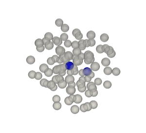
Consider the problem of two particles (denoted 1 and 2) separated by a distance $d$ along $x_1$ and surrounded by other random distribution of particles with uniform probability corresponding to a volume fraction of $\alpha$. Given the two particles, there are infinite possibilities for the arrangement of the other particles. Two realizations are shown in figure 14. The velocity potential in realization $\omega$ satisfies

(5.6)\begin{equation} I_\omega(\boldsymbol{x)} \nabla^2 (\phi_\omega(\boldsymbol{x})) = 0, \end{equation}

where $I_\omega ({\boldsymbol {x}})$ is the indicator function of that realization and it is unity in regions occupied by the fluid and zero inside particles. We then perform an ensemble average over all realizations similar to those shown in figure 14, which upon manipulation yields (Balachandar Reference Balachandar2024)

(5.7)\begin{equation} \nabla^2 (\langle I \rangle (\boldsymbol{x)} \langle \phi \rangle (\boldsymbol{x})) ={-}\nabla^2 (\langle I' \phi' \rangle (\boldsymbol{x})) + \langle \boldsymbol{u} \boldsymbol{\cdot} \boldsymbol{n} \rangle + \boldsymbol{\nabla}\boldsymbol{\cdot} \langle \phi \boldsymbol{n} \rangle = 0. \end{equation}

On the left-hand side, $\langle I \rangle$ is the ensemble-averaged fluid volume fraction, given the position of the two particles denoted as 1 and 2, and the average volume fraction. This can be shown to be related to the three-particle radial distribution function (Torquato & Haslach Jr Reference Torquato and Haslach2002). On the right-hand side, $I'$ and $\phi '$ are perturbations away from the mean. The last two terms on the right-hand side are interface terms that are non-zero only on the surface of the particles. Here, $\boldsymbol {u} \boldsymbol {\cdot } \boldsymbol {n}$ is the particle velocity along the surface normal $\boldsymbol {n}$. Once computed, $\langle \phi \rangle$ can be used to calculate the ensemble-averaged velocity and using the Bernoulli equation the ensemble-averaged pressure, which can be integrated to obtain the functions $\mathcal {B}^{c11}_{11}(d,\alpha )$, $\mathcal {B}^{c11}_{22}(d,\alpha )$, $\mathcal {B}^{c12}_{11}(d,\alpha )$ and $\mathcal {B}^{c12}_{22}(d,\alpha )$.

Figure 14.

Two realizations ($\omega =1$, and $2$), where two particles are held fixed in their position and the location of all other neighbours in blue are randomly varied to follow uniform distribution at the desired volume fraction. Panels show (a) $\omega =1$, (b) $\omega =2$.

However, it is not easy to solve (5.7) because of the unclosed terms on the right-hand side. Instead, here we obtain the $\alpha$-corrected functions in the following way using the potential flow we earlier computed for $N=1000$ particles. A system of $N$ particles randomly distributed in a triply periodic box consists of $N(N-1)/2$ unique particle pairs, with each pair surrounded by a unique distribution of neighbours. The distance between the particles within a pair varies between $d=2a$ to $d = ({\rm \pi} N/(6\alpha ))^{1/3} a$. For each particle pair, by rotating the coordinates so that the particle pair lies along the $x_1$-axis, the computed potential flow can be converted to the desired solution of (5.6) for an individual realization of the particle pair. Furthermore, the method of images used to calculate the potential flow allows for the precise extraction of the following two quantities.

Added mass perturbation: for each pair, we seek the potential flow generated at particle-1 because of particle-1's acceleration. Therefore, we restrict to only those doublets whose associated original doublet is that of particle-1 and as a result, their contributions multiply particle-1's acceleration. Furthermore, we want to focus only on those doublets that account for direct modification by particle-2, but in the presence of indirect influence of all other particles. This restriction is accomplished with the following two conditions: (i) the doublet is located within particle-2 or (ii) the doublet is located within particle-1, but its most recent reflection is from particle-2. The added mass tensor of particle-1 evaluated in this manner using (2.17) with the restricted set of doublets. The tensor is then rotated so that the line separating the two particles is oriented along $x_1$. The rotated added mass tensor will not be perfectly axisymmetric due to the complex indirect interaction of other randomly distributed particles. But the (1,1) element of the tensor can be interpreted as added mass perturbation of $x_1$-force of particle-1 due to its $x_1$-acceleration due to the direct influence of particle-2. The (2,2) and (3,3) elements of the tensor can be interpreted as the perturbation of particle-1's perpendicular added mass force due to its perpendicular acceleration due to the direct influence of particle-2. They will be denoted as $B^{11}_{11}$ and $B^{11}_{22}$.

Scatter plots of $B^{11}_{11}$ and $B^{11}_{22}$ as a function of $d$ for all particle pair combinations are presented in figure 15(a,b). In the limit of $\alpha \rightarrow 0$ (i.e. in the absence of all other particles) the data points lie on a single curve corresponding to that of two isolated particles presented in figure 10. For $\alpha \ne 0$, the data points do not fall on a line due to randomness in the distribution of other particles. By taking an ensemble average over all possible arrangements of the other particles we define

(5.8a,b)\begin{equation} \mathcal{B}^{c11}_{11} = \langle B^{11}_{11} \rangle \quad \mbox{and} \quad \mathcal{B}^{c11}_{22} = \langle B^{11}_{22} \rangle . \end{equation}

The curve fits representing these ensemble averages are presented in Appendix C and also shown as lines in figure 15. The $\alpha$ dependence appears to be quite small and hard to discern in the plot. Nevertheless, we observe this small volume fraction correction applies to all binary interactions with neighbours and therefore is necessary to accurately capture the mean binary perturbation.

Figure 15.

Binary model as a function of distance, $d$, and volume fraction, $\alpha$, extracted from the exact resistance matrices. The points are the values extracted from the method of images and the lines are empirical curve fits to these data. The panels include the following variables: (a) $B^{11}_{11}$, (b) $B^{11}_{22}$, (c) $B^{12}_{11}$ and (d) $B^{12}_{22}$.

Induced mass perturbation: for each pair, we now seek the potential flow generated at particle-1 because of particle-2's acceleration. Therefore we restrict to only those doublets whose associated original doublet is that of particle-2. No further restrictions are necessary. The induced mass tensor of particle-1 is evaluated using (2.17) with the restricted set of doublets. The tensor is then rotated so that the line separating the two particles is oriented along $x_1$. The rotated tensor is again not perfectly axisymmetric. The (1,1) element can be interpreted as the induced mass perturbation of $x_1$-force of particle-1 due to the $x_1$-acceleration of particle-2. The (2,2) and (3,3) elements can be interpreted as the perturbation of particle-1's perpendicular added mass force due to the perpendicular acceleration of particle-2. They will be denoted as $B^{12}_{11}$ and $B^{12}_{22}$.

Scatter plots of $B^{12}_{11}$ and $B^{12}_{22}$ as a function of $d$ for all particle pair combinations is presented in figure 15(c,d). In the limit of $\alpha \rightarrow 0$, the data points lie on a curve corresponding to that of two isolated particles presented in figure 10. For $\alpha \ne 0$, the data points exhibit a scatter due to randomness in the distribution of other particles. Taking an ensemble average over all possible arrangements of the other particles we define

(5.9a,b)\begin{equation} \mathcal{B}^{c12}_{11} = \langle B^{12}_{11} \rangle \quad \mbox{and} \quad \mathcal{B}^{c12}_{22} = \langle B^{12}_{22} \rangle. \end{equation}

The curve fits representing these ensemble averages are presented in Appendix C and also shown as lines in figure 15. In these plots, the $\alpha$-dependence can be readily observed. It should be noted that these $\alpha$-dependent pair-interaction functions also depend on the nature of particle distribution. Here, we have obtained them for a uniform random distribution of particles that obey the canonical $3\varGamma$ Voronoi volume distribution.

5.4. Improved accuracy of the $\alpha$-corrected binary model

The four $\alpha$-corrected binary interaction functions given in (C1), (C2), (C3) and (C4) can now be used in (5.2a,b) and (5.3a,b) to obtain the corrected added and induced mass tensors $\underline {\underline {B}}^{cA}$ and $\underline {\underline {B}}^{cI}$. This can then be substituted in (5.4) to evaluate the added mass matrix of a random distribution of particles given their position and acceleration. Let us denote the resulting $\alpha$-corrected binary added mass matrix as $\underline {\underline {\tilde {R}}}^c$. In this subsection, we will assume that the corrected binary model is computed to sufficient accuracy and that the only error committed is in the neglect of trinary and higher-order effects. For this, we observe it is sufficient to consider all the neighbours within a sphere of radius $\mathcal {R}_{max} = 10a$.

The $9N^2$ elements of the added mass matrix $\underline {\underline {\tilde {R}}}^c$ were calculated with the corrected binary model. Figures 16 and 17 show the scatter plot of the off-diagonal and diagonal block elements of the $\alpha$-corrected model plotted against the exact results of the potential flow solution. The corrected binary model is able to quite accurately predict all the elements of the exact added mass matrix. Especially, the underprediction of both the mean and standard deviation at higher values of $\alpha$ has been corrected. In addition to better capturing the individual elements of the resistance matrix, figure 18 shows that the corrected model is able to reproduce the added mass force statistics of a rigidly accelerating cloud. The higher-order moments (not shown) are also reasonably well produced.

Figure 16.

Off-diagonal ($i \neq j$) entries of the resistance matrix predicted by the corrected binary model, $\tilde {R}^c_{ij}$, plotted against the entries of the exact resistance matrix, $R_{ij}$, as a function of volume fraction, $\alpha$, and maximum interaction distance, $\mathcal {R}_{max}/a$. Each point represents one entry in the resistance matrix. The vertical lines indicate the maximum and minimum exact values that have been neglected in the binary model due to a neighbour being beyond $\mathcal {R}_{max}$. The binary model correction is calculated using the analytic expression for $g(r)$ provided by Trokhymchuk et al. (Reference Trokhymchuk, Nezbeda, Jirsák and Henderson2005). Panels show (a) $\alpha =0.001$, (b) $\alpha =0.05$, (c) $\alpha =0.1$, (d) $\alpha =0.2$, (e) $\alpha =0.4$.

Figure 17.

Diagonal ($i= j$) entries of the resistance matrix predicted by the corrected binary model, $\tilde {R}^c_{ij}$, plotted against the entries of the exact resistance matrix, $R_{ij}$, as a function of volume fraction, $\alpha$, and maximum interaction distance, $\mathcal {R}_{max}/a$. Each point represents one entry in the resistance matrix. The vertical lines indicate the maximum and minimum exact values that have been neglected in the binary model due to a neighbour being beyond $\mathcal {R}_{max}$. The binary model correction is calculated using the analytic expression for $g(r)$ provided by Trokhymchuk et al. (Reference Trokhymchuk, Nezbeda, Jirsák and Henderson2005). Panels show (a) $\alpha =0.001$, (b) $\alpha =0.05$, (c) $\alpha =0.1$, (d) $\alpha =0.2$, (e) $\alpha =0.4$.

Figure 18.

Statistics of parallel (drag-like) and perpendicular (lift-like) added mass coefficients as a function of volume fraction, $\alpha$. The system is assumed to accelerate rigidly such that $\sigma _{\dot {V}}=0$. The statistics reported are (a) mean, and (b) standard deviation. The points plotted are the prediction by the corrected binary model, while the lines represent the results from the $N$-body potential flow computation. This version of the corrected model used the relation of Trokhymchuk et al. (Reference Trokhymchuk, Nezbeda, Jirsák and Henderson2005) to calculate $g(r)$, as explained in § 5.5.

5.5. Corrected binary model for limited nearby neighbours

On average, a neighbourhood of $\mathcal {R}_{max} = 10a$ includes roughly 400 neighbours for $\alpha =0.4$. To reduce the substantial computational cost of calculating the binary effect of a large number of neighbours, it is desirable to limit the value of $\mathcal {R}_{max}$. Tests reveal that the accuracy of the $\alpha$-corrected model suffers substantially as $\mathcal {R}_{max}$ falls much below $10a$. In this section, we present a simple approach that allows for the $\alpha$-corrected model to perform accurately even for smaller values of $\mathcal {R}_{max}$ without significant loss of accuracy. In this approach, the neighbours will be separated into near-field neighbours whose centres are within the annular region $2a \le |\boldsymbol{r}^{p,s}| < \mathcal {R}_{max}$ and far-field neighbours whose centres are within the annular region $\mathcal {R}_{max} \le |\boldsymbol{r}^{p,s}|$. The near-field influence will be calculated deterministically with the precise knowledge of all neighbours that lie within a sphere of radius $\mathcal {R}_{max}$ using the expression given (5.4). The far-field influence must then be calculated in a statistical sense without the precise knowledge of the outlying neighbours.

According to the binary model, the far-field neighbours’ influence on particle-1 can be separated into (i) the added mass perturbation that gets multiplied by particle-1's acceleration and (ii) the induced mass perturbation that gets multiplied by the acceleration of the far-field particles. Without the knowledge of the exact locations of the far-field neighbours, we assume the particles to be uniformly distributed outside the sphere of radius $\mathcal {R}_{max}$. With this assumption, the added mass and induced mass effects on particle-1 can be expressed as

(5.10)\begin{equation} \underline{\underline{I}}^A = \underline{\underline{I}} \int_{r/a=\mathcal{R}_{max}/a}^\infty (r/a)^2 \alpha g(r/a) [\mathcal{B}_{11}^{c11} (r/a, \alpha) + 2 \mathcal{B}_{22}^{c11} (r/a, \alpha)]\,{\rm d}(r/a), \end{equation}

and

(5.11)\begin{equation} \underline{\underline{I}}^I = \underline{\underline{I}} \int_{r/a=\mathcal{R}_{max}/a}^\infty (r/a)^2 \alpha g(r/a) [\mathcal{B}_{11}^{c12} (r/a, \alpha) + 2 \mathcal{B}_{22}^{c12} (r/a, \alpha)]\,{\rm d}(r/a), \end{equation}

where $\underline {\underline {I}}$ is the identity matrix and $g(r/a)$ is the radial distribution function that measures the relative probability of finding a neighbour at a radial distance of $r$ from particle-1 compared with the uniform probability. In the above, we have used the relations

(5.12)\begin{equation} \left.\begin{gathered} \oint_{S_\mathcal{R}} \underline{\underline{Q}}^\top \underline{\underline{\mathcal{B}}}^{c11} \underline{\underline{Q}} \,{\rm d} A = \frac{4 {\rm \pi}}{3}[\mathcal{B}_{11}^{c11} (r/a, \alpha) + 2 \mathcal{B}_{22}^{c11} (r/a, \alpha)] \underline{\underline{I}} \\ \oint_{S_\mathcal{R}} \underline{\underline{Q}}^\top \underline{\underline{\mathcal{B}}}^{c12} \underline{\underline{Q}} {\rm d} A = \frac{4 {\rm \pi}}{3}[\mathcal{B}_{11}^{c12} (r/a, \alpha) + 2 \mathcal{B}_{22}^{c12} (r/a, \alpha)] \underline{\underline{I}},\end{gathered}\right\} \end{equation}

where the integrations are over a surface of radius $r$. In figure 10 it was noted that, while $\underline {\underline {\mathcal {B}}}^{c11}$ decayed faster, the induced mass effect $\underline {\underline {\mathcal {B}}}^{c12}$ decayed only as $1/r^3$. Nevertheless, as discussed previously in § 5.1, the leading-order terms in the induced added mass integral cancel exactly so that the integral converges.

In the case of $\underline {\underline {I}}^A$, it will be multiplied by the acceleration vector of the particle whose added mass force is being evaluated and therefore can be combined with the diagonal blocks of the added mass matrix. In contrast, $\underline {\underline {I}}^I$ must be multiplied by the average acceleration of the far-field particles, which is not readily available to the $\alpha$-corrected binary model and therefore must be approximated. There are several modelling choices and the best option will depend on the problem. For example, the average acceleration of the far-field particles may be simply taken to be that of the particle whose added mass force is being evaluated. In which case, $\underline {\underline {I}}^I$ can also be combined with the diagonal blocks of the added mass matrix. An alternate model will be to assume the average acceleration of the far-field particles to the average of all the near-field neighbours. In this latter approximation $\underline {\underline {I}}^I$ will be equally distributed to the blocks that are associated with the near-field neighbours. Here, we will pursue this latter modelling choice and the resulting $\alpha$-corrected binary model of the added mass matrix can be expressed as

(5.13)\begin{equation} \tilde{R}_{3(s-1)+i,3(p-1)+j}^c = \begin{cases} \dfrac{1}{2} \delta_{ij} + \displaystyle\sum_{\substack{r=1 \\ r\neq s}}^{N_R} B^{cA}_{ij} (\boldsymbol{r}^{rs}) + {I}^A_{ij} & \mbox{if}\ p=s \\ B^{cI}_{ij} (\boldsymbol{r}^{ps}) + \dfrac{1}{N_R} {I}^I_{ij} & \mbox{if}\ p \ne s, \end{cases} \end{equation}

where $N_R$ is the number of neighbours within a radius of $\mathcal {R}_{max}$, and

(5.14a,b)\begin{equation} \underline{\underline{B}}^{cA} = \underline{\underline{Q}}^\top \underline{\underline{\mathcal{B}}}^{c11} \underline{\underline{Q}}\quad \mbox{and}\quad \underline{\underline{B}}^{cI} = \underline{\underline{Q}}^\top \underline{\underline{\mathcal{B}}}^{c12} \underline{\underline{Q}}. \end{equation}

Using the analytical expression for $g(r)$ derived by Trokhymchuk et al. (Reference Trokhymchuk, Nezbeda, Jirsák and Henderson2005) appropriate for uniform distribution of hard spheres, $\textrm {tr}\{{I}^A\}/3$ and $\textrm {tr}\{{I}^I\}/3$ were evaluated by computing the integrals given in (5.10) and (5.11) and plotted in figure 19. Also shown are analytical expressions obtained assuming $g(r)=1$ (see Appendix D). As expected, both $\textrm {tr}\{{I}^A\}/3$ and $\textrm {tr}\{{I}^I\}/3$ decay with increasing $\mathcal {R}_{max}$ and are not needed for $\mathcal {R}_{max} \gtrapprox 8a$. Furthermore, as long as $\mathcal {R}_{max} \gtrapprox 3.5a$ the analytic expressions given in Appendix D that assume $g(r) = 1$ are sufficient.

Figure 19.

Integral corrections for the mean added mass force evaluated using the analytical approximation assuming $g(r)=1$ as outlined in Appendix D compared with the numerically integrated values using $g(r)$ from Trokhymchuk et al. (Reference Trokhymchuk, Nezbeda, Jirsák and Henderson2005). The numerically integrated values are shown as points and the approximate analytic values are shown as lines. The panels show (a) the self-acceleration component, and (b) the induced component.

The resistance matrix of the $\alpha$-corrected binary model $\tilde {R}^c_{ij}$ was computed for several values for $\mathcal {R}_{max} < 10$ using (5.13). These results are also presented in figures 16 and 17 for the diagonal and off-diagonal terms, which were earlier discussed in the limit $\mathcal {R}_{max} = 10$ when the model did not need to include the additional contributions from ${I}^A$ and ${I}^I$. With decreasing $\mathcal {R}_{max}$, the model performance slightly decreases, nevertheless, the performance is quite reasonable for all values considered, especially when compared with that of the uncorrected model results presented in figures 11 and 12. The mean and standard deviation of parallel and perpendicular components of added mass force on a random distribution of particles subjected to uniform acceleration was computed with (5.13) and presented in figure 18 for different values of $\mathcal {R}_{max}$. It is quite clear that the $\alpha$-corrected model with the inclusion of statistical contribution of far-field neighbours is quite accurate, except perhaps for $\mathcal {R}_{max}=3a$ and large volume fraction values. It should be pointed out for $\mathcal {R}_{max} \gtrapprox 3.5a$ the analytical expressions given in Appendix D obtained using $g(r) = 1$ are quite accurate.

As a further test of the model, the maximum and r.m.s. errors are shown in figure 20 to quantify the error in the $\alpha$-corrected model. At each volume fraction, ten realizations are considered and the average value of the different error metrics defined in (3.1a,b) are plotted along with their extreme values as error bars. Focusing on the maximum error presented in figure 20(a), we observe that the error increases with volume fraction. This can be expected since more particles will be close to one another at higher volume fractions thereby making the specifics of trinary and higher-order terms more significant than their average effects. Furthermore, increasing $\mathcal {R}_{max}/a$ beyond 6 does not yield any additional decrease in maximum error except at very small volume fractions where the maximum error is already low. The maximum error seems to be under 10 % for all the selected interaction distances. Despite this invariance of the maximum error with changing $\mathcal {R}_{max}$, figure 20(b) indicates that there is an improvement in the r.m.s. error with increasing $\mathcal {R}_{max}$. Here, we notice a consistent improvement in error with increasing interaction distance. As expected, the r.m.s. error is consistently small which indicates that most of the terms in the resistance matrix are well predicted by the $\alpha$-corrected binary model.

Figure 20.

Maximum (a) and r.m.s. (b) error for predicting a 1000 particle system using the corrected binary model. The points plotted are the mean error for 10 realizations and the error bars indicate the maximum and minimum errors for the 10 realizations. Here, $\mathcal {R}_{max}/a$ is the maximum radius within which neighbouring particles were considered for evaluating the binary model. The relation for the radial distribution function, $g(r)$, provided by Trokhymchuk et al. (Reference Trokhymchuk, Nezbeda, Jirsák and Henderson2005) was used.