1 Introduction
To understand turbulent boundary layer flows has always been among the research focuses of the turbulence community. It is widely accepted that in turbulent boundary layers there exist both organized and disorganized motions. The organized part can be characterized by appropriate geometrical descriptions, for instance coherent structures with multi-scales in both space and time. In the near-wall region of a turbulent boundary layer, the dominant dynamic modes are rolls and low-speed streaks (Kline et al. Reference Kline, Reynolds, Schraub and Runstadler1967; Kim, Moin & Moser Reference Kim, Moin and Moser1987; Robinson Reference Robinson1991). Jimenez & Pinelli (Reference Jimenez and Pinelli1999) analysed the possible mechanisms of turbulence production in this region. In the log region and outer wake regions, the inclined hairpin vortex structure has been extensively studied (Head & Bandyopadhyay Reference Head and Bandyopadhyay1981; Zhou et al. Reference Zhou, Adrian, Balachandar and Kendall1999; Adrian Reference Adrian2007; Kang, Choi & Chun Reference Kang, Choi and Chun2008; Wu & Moin Reference Wu and Moin2009). Adrian, Meinhart & Tomkins (Reference Adrian, Meinhart and Tomkins2000) further found that the hairpin vortices can also appear as a group, which is termed a hairpin packet. At relatively high Reynolds numbers, Kim (Reference Kim and Adrian1999) proposed the existence of highly energetic very-large-scale structures, which have been verified in subsequent studies (Abe, Kawamura & Choi Reference Abe, Kawamura and Choi2004; Ganapathisubramani, Clemens & Dolling Reference Ganapathisubramani, Clemens and Dolling2006; Monty et al. Reference Monty, Stewart, Williams and Chong2007; Marusic & Hutchins Reference Marusic and Hutchins2008). There are also interesting theoretical investigations of the so-called exact coherent structures (Waleffe Reference Waleffe1997; Brandt, Henningson & Ponziani Reference Brandt, Henningson and Ponziani2002; Skufca, Yorke & Eckhardt Reference Skufca, Yorke and Eckhardt2006; Deguchi & Hall Reference Deguchi and Hall2014).
Coherent structures play an important role in heat transfer and flow drag control. To elucidate the dynamical behaviour of the coherent structures, several techniques have been proposed, including conditional sampling (Antonia Reference Antonia1981), pattern recognition (Eckelmanns et al. Reference Eckelmanns, Nychas, Brodkey and Wallace1977), proper orthogonal decomposition (POD) (Karhunen Reference Karhunen1946), spatial correlations (Ganapathisubramani et al. Reference Ganapathisubramani, Clemens and Dolling2006; Chen et al. Reference Chen, Hussain, Pei and She2014; Mouri Reference Mouri2017), Lagrangian coherent structures (Haller Reference Haller2015; Schlueter-Kuck & Dabiri Reference Schlueter-Kuck and Dabiri2017) and the vortex-surface field method (Yang & Pullin Reference Yang and Pullin2011; Zhao, Yang & Chen Reference Zhao, Yang and Chen2016). In spite of these numerous efforts, the coherent structures and multi-scale turbulent motions are still not well understood. In summary, the following fundamental issues in structure and geometry analysis need to be addressed:
(i) How can structures be quantitatively and unbiasedly defined, rather than qualitatively described? For instance, the well-studied hairpin vortices, although they can be nicely visualized, are defined with arbitrariness in choosing the contour values. Meanwhile, because by volume such vortices take up only a small portion of the entire flow field, i.e. they are not space-filling, it is not reasonable to understand the entire flow only from the behaviour of hairpin vortices.
(ii) Statistically, how can structures be sufficiently characterized, but in a relatively simple way? Theoretically, flow structures are infinite-dimensional, which makes it is inapplicable to list exhaustively the geometrical parameters of relevance. It is an important prerequisite to reduce the structure dimensionality, at the same time without oversimplification of the physical meaningfulness.
(iii) How can the structure characterization be applied to flow analysis? To achieve this, it is necessary to extract proper characteristic parameters, such as the spatial scale and the flow structure. Considering the scale, for instance, the Fourier representation in wavelength space can be implemented, which in principle is reasonable only for isotropic turbulence. In more complex flows, such as the turbulent boundary layer case (inhomogeneous in the wall-normal direction), the spectral method will then lead to inherent complications associated with the presence of a wall. Therefore it is fundamentally meaningful to characterize the flow structures in a more general sense.
Without a good understanding of these issues, it is difficult to further develop structure analysis beyond illustration and description. Fortunately, in the past decade, some enlightening progress has been made in this framework. For turbulent scalar variables, Wang & Peters (Reference Wang and Peters2006) proposed the dissipation element structure to partition a scalar field into space-filling and non-overlapping units, named dissipation elements. Each element consists of grid points whose scalar gradient trajectories share the same local minimum and maximum of the scalar quantity under consideration. Based on such spatial decomposition, the original complex system can be better understood from the statistics of the relatively simple units. In principle, dissipation element analysis functions for different scalar fields (Wang & Peters Reference Wang and Peters2008) and different flowing cases, such as isotropic turbulence and turbulent jet mixing (Gampert et al. Reference Gampert, Goebbert, Schaefer, Gauding, Peters, Aldudak and Oberlack2011; Gampert, Schaefer & Peters Reference Gampert, Schaefer and Peters2013). For the velocity vector case, Wang (Reference Wang2010) developed streamline segment analysis, by which the turbulent velocity field can be decomposed into non-overlapping streamline segments. As will be explained in the next section, streamline segments can be either positive or negative. A main conclusion is that the skewness of velocity derivatives is naturally the kinematic evolution consequence because of the asymmetry between the positive and negative groups. In principle, the streamline segment idea can be implemented directly to different vector quantities. For more application examples and relevant progress, readers are referred to Wang (Reference Wang2012), Schaefer, Gampert & Peters (Reference Schaefer, Gampert and Peters2013), Boschung et al. (Reference Boschung, Schaefer, Peters and Meneveau2014) and Wang (Reference Wang2014).
The main focus of the present work is to investigate the turbulent boundary layer structure. Here we choose a canonical configuration of the boundary flow over a flat plate with zero streamwise pressure gradient, which from the viewpoint of fundamental research represents the simplest case in many respects. The turbulent boundary layer structure will then be analysed in a quantitative and unbiased manner using vectorline segment analysis. A similar idea can generally be applied to study more complicated features such as very-large-scale motions at high Reynolds numbers.
2 Direct numerical simulations
Direct numerical simulations (DNS) of turbulent flow over a zero-pressure-gradient flat plate is performed. The three-dimensional unsteady compressible Navier–Stokes equations for a perfect gas cast in a conservative form are solved using a finite difference approach. The viscous terms and convective terms are evaluated by a sixth-order central difference scheme and a sixth-order compact difference scheme in transformed curvilinear coordinates (Lele Reference Lele1992; Visbal & Gaitonde Reference Visbal and Gaitonde2002), respectively. To ensure numerical stability an eighth-order low-pass spatial filtering (with the optimization parameter
 $\unicode[STIX]{x1D6FC}_{f}=0.493$
) (Lele Reference Lele1992) is applied at each time step on the conservative variables. An alternate directional implicit symmetric Gauss–Seidel (ADI-SGS) scheme (Nishida & Nonomura Reference Nishida and Nonomura2009) is used for the temporal integration with three local sub-iterations to converge the Newton–Raphson sub-iterative process, which can lead to a second-order temporal accuracy. The computational fluid dynamics (CFD) solver has been extensively validated in previous works, for instance for wall-bounded turbulent flows and free jet flows (Nonomura & Fujii Reference Nonomura and Fujii2011; Li, Nonomura & Fujii Reference Li, Nonomura and Fujii2013a
,Reference Li, Nonomura and Fujii
b
).
No-slip and adiabatic boundary conditions are imposed at the bottom wall, and the zero-pressure-gradient condition is used at the outlet and the upper boundary. A recycling and rescaling technique is utilized at the inlet to generate fully developed turbulence without considering a laminar-to-turbulent transition. Specifically, by decomposing the flow field into a time-averaged part and a fluctuating part, the flow properties downstream are recycled to the inlet as the inflow boundary condition according to an appropriate scaling law (Pirozzoli, Bernardini & Grasso Reference Pirozzoli, Bernardini and Grasso2008). The mean flow field at the inflow is obtained from a two-dimensional Reynolds-averaged Navier–Stokes (RANS) simulation of a flat plate with Spalart–Allmaras turbulence model (Spalart & Allmaras Reference Spalart and Allmaras1992). A weighted function, which was proposed by Lund, Wu & Squires (Reference Lund, Wu and Squires1998), is used to combine the inner- and outer-layer fluctuations. To avoid numerical ‘drift’ (as discussed in Sagaut et al. (Reference Sagaut, Garnier, Tromeur, Larcheveque and Labourasse2012)), the mean flow fields at the inlet are kept constant, and only the flow density and velocity fluctuations are recycled and rescaled. A dynamic reflection operation proposed by Morgan et al. (Reference Morgan, Larsson, Kawai and Lele2011) is applied to eliminate the downstream spurious spatial correlations and reduce unphysical temporal correlations related to the recycling procedure. To more efficiently reach statistically stationary turbulence, the velocity field is initialized using a similar approach developed by Sandham, Yao & Lawal (Reference Sandham, Yao and Lawal2003) and Pirozzoli et al. (Reference Pirozzoli, Bernardini and Grasso2008). At the statistically stationary state, data samples in a time span of approximately
 $90\unicode[STIX]{x1D6FF}_{in}/U_{\infty }$
are collected for analysis. As justified in the Appendix, such sampling time span is sufficient for statistical convergence.
In the present simulation, the free-stream Mach number is set as
 $M=U_{\infty }/a_{\infty }=0.3$
in the incompressible regime (Kawai Reference Kawai2016), where
 $U$
is the streamwise velocity component,
 $a$
is the speed of sound, and the subscript
 $\infty$
denotes the free-stream properties. The Reynolds number based on
 $U_{\infty }$
and inlet velocity boundary layer thickness
 $\unicode[STIX]{x1D6FF}_{in}$
is
 $Re_{\unicode[STIX]{x1D6FF}_{in}}=1.1\times 10^{4}$
, corresponding to
 $Re_{\unicode[STIX]{x1D703}}=1300$
(based on the momentum boundary layer thickness). To ensure the Courant–Friedrichs–Lewy (CFL) number less than unity, the time step
 $\unicode[STIX]{x1D6FF}t$
is set as
 $\unicode[STIX]{x1D6FF}t=3\times 10^{-4}\,\unicode[STIX]{x1D6FF}_{in}/U_{\infty }$
. Because the change of the boundary layer thickness from inlet to outlet is negligibly small (approximately 1 %), in the following analysis the flow is considered as homogeneous in the streamwise direction. With respect to the viscous units, the viscous time step
 $\unicode[STIX]{x1D6FF}t^{+}=\unicode[STIX]{x1D6FF}t\,u_{\unicode[STIX]{x1D70F}}^{2}/\unicode[STIX]{x1D708}$
is less than 0.004, where
 $u_{\unicode[STIX]{x1D70F}}$
denotes the wall friction velocity and
 $\unicode[STIX]{x1D708}$
is the kinematic viscosity. The size of the computational domain is
 $L_{x}\times L_{y}\times L_{z}=11\unicode[STIX]{x1D6FF}_{in}\times 1.7\unicode[STIX]{x1D6FF}_{in}\times 3\unicode[STIX]{x1D6FF}_{in}$
, where
 $x$
,
 $y$
and
 $z$
stand for the streamwise, wall-normal and spanwise directions, respectively. In total there are
 $N_{x}\times N_{y}\times N_{z}=764\times 179\times 251$
grid points, which are uniformly distributed in the streamwise direction with
 $\unicode[STIX]{x1D6FF}x^{+}=6$
and spanwise direction with
 $\unicode[STIX]{x1D6FF}z^{+}=5$
, while smoothly stretched in the wall-normal direction from
 $\unicode[STIX]{x1D6FF}y^{+}=0.85$
at the wall to
 $\unicode[STIX]{x1D6FF}y^{+}=5$
at the boundary layer edge, where
 $y^{+}\approx 410$
. As discussed in the Appendix, such resolution is fine enough for the following statistical analyses. In addition, to avoid fluctuations and any reflections from the outlet and the upper boundary, a buffer (sponge) domain is designed, which extends
 $12\unicode[STIX]{x1D6FF}_{in}$
with 50 grid points and
 $25\unicode[STIX]{x1D6FF}_{in}$
with 40 grid points in the streamwise and wall-normal directions, respectively.
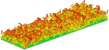
Figure 1 shows an instantaneous snapshot of an isosurface of the second invariant of the complete velocity gradient tensor, coloured with the magnitude of the streamwise velocity. The hairpin structure conforms to the existing literature results. The structure scale evolves to be larger along the wall-normal direction.
Instantaneous snapshot of an isosurface of the second invariant of the complete velocity gradient (
 $Q=0.5$
), coloured by the streamwise velocity (
 $0\leqslant u\leqslant 0.32$
).

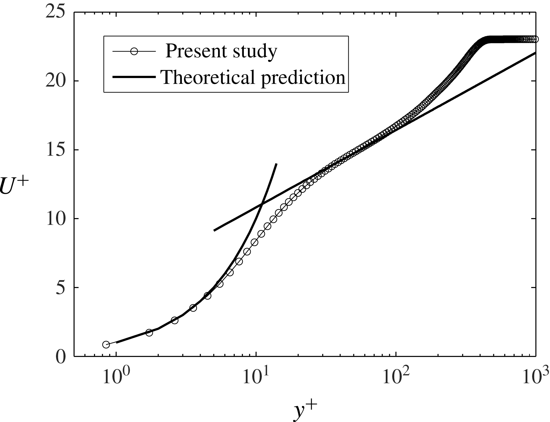
To validate the simulation results, figure 2 shows the time-averaged streamwise velocity profile in a semi-logarithmic plot. It can be seen that the present DNS result agrees well with the standard theoretical prediction both in the viscous sublayer as
 $U^{+}=y^{+}$
and in the log-layer region
 $U^{+}=2.4\log (y^{+})+5.2$
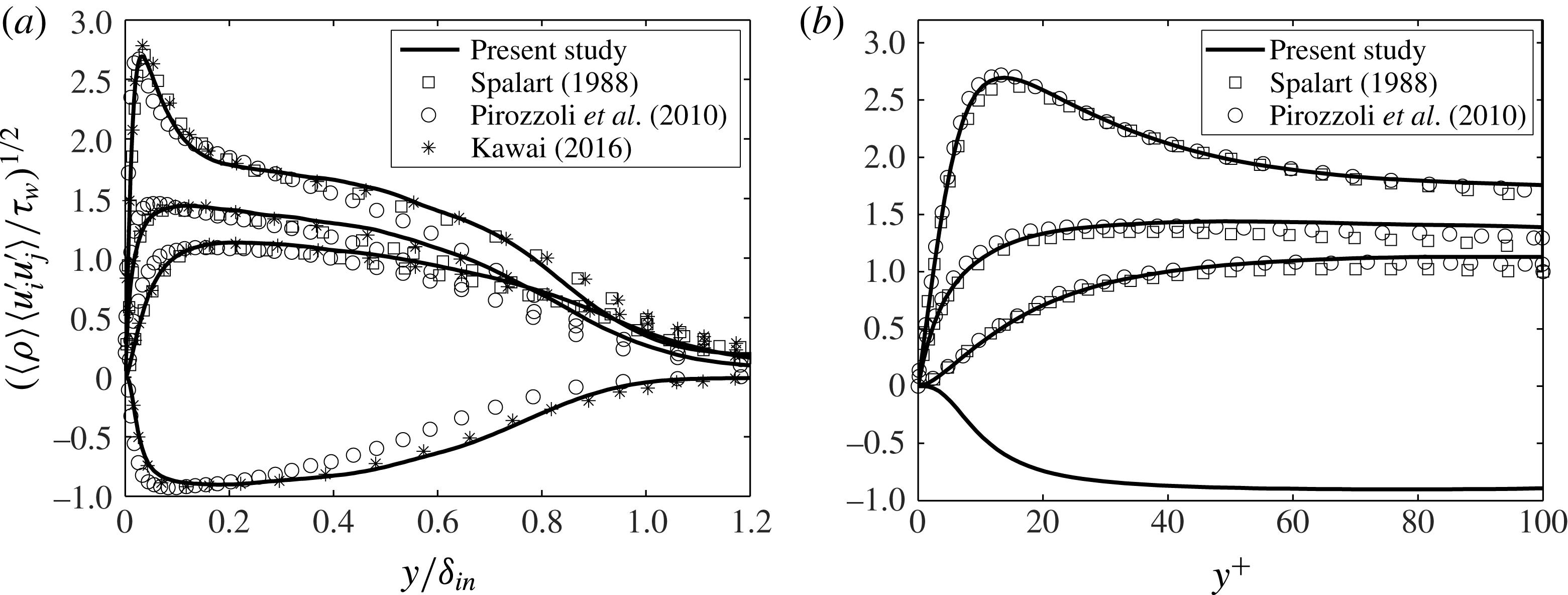
. Figure 3 shows the distribution of Reynolds stress components in both inner scaling and outer scaling, which are in good agreement with the incompressible DNS results at
 $Re_{\unicode[STIX]{x1D703}}=1410$
(Spalart Reference Spalart1988), supersonic DNS data at
 $M=1.4$
and
 $Re_{\unicode[STIX]{x1D703}}=1215$
(Pirozzoli, Bernardini & Grasso Reference Pirozzoli, Bernardini and Grasso2010), and compressible subsonic DNS data at
 $M=0.3$
and
 $Re_{\unicode[STIX]{x1D703}}=1010$
(Kawai Reference Kawai2016).
Profile of the time-averaged streamwise velocity in wall units.

Comparison of the calculated Reynolds stress components from the present DNS data (solid line) and the literature results (▫, Spalart (Reference Spalart1988); ○, Pirozzoli et al. (Reference Pirozzoli, Bernardini and Grasso2010); *, Kawai (Reference Kawai2016)) in (a) inner scaling and (b) outer scaling for: (top) the streamwise component (
 $i=j=1$
); (upper middle) the spanwise component (
 $i=j=3$
); (lower middle) the wall-normal component (
 $i=j=2$
); and (bottom) the Reynolds shear stress (
 $i=1$
,
 $j=2$
).

Following the incompressibility condition, a generic form of the turbulent kinetic energy transport equation is formulated as
 $$\begin{eqnarray}\frac{\text{D}k}{\text{D}t}=P+T+D+\unicode[STIX]{x1D716},\end{eqnarray}$$
where the turbulent kinetic energy is defined as
 $k=\langle u_{i}^{\prime }u_{i}^{\prime }\rangle /2$
. The production term
 $P$
, the transport term (by velocity fluctuations and velocity–pressure interaction)
 $T$
, the viscous diffusion term
 $D$
and the dissipation term
 $\unicode[STIX]{x1D716}$
, respectively, are expressed as
 $$\begin{eqnarray}\displaystyle & \displaystyle P=-\langle u_{i}^{\prime }u_{j}^{\prime }\rangle \frac{\unicode[STIX]{x2202}\langle u_{j}\rangle }{\unicode[STIX]{x2202}x_{i}}, & \displaystyle\end{eqnarray}$$
 $$\begin{eqnarray}\displaystyle & \displaystyle T=-\frac{\unicode[STIX]{x2202}}{\unicode[STIX]{x2202}x_{i}}\left\langle u_{i}^{\prime }\left(\frac{p^{\prime }}{\unicode[STIX]{x1D70C}}+\frac{1}{2}u_{i}^{\prime }u_{i}^{\prime }\right)\right\rangle , & \displaystyle\end{eqnarray}$$
 $$\begin{eqnarray}\displaystyle & \displaystyle D=\unicode[STIX]{x1D708}\frac{\unicode[STIX]{x2202}}{\unicode[STIX]{x2202}x_{i}}\left\langle u_{j}^{\prime }\left(\frac{\unicode[STIX]{x2202}u_{i}^{\prime }}{\unicode[STIX]{x2202}x_{j}}+\frac{\unicode[STIX]{x2202}u_{j}^{\prime }}{\unicode[STIX]{x2202}x_{i}}\right)\right\rangle , & \displaystyle\end{eqnarray}$$
 $$\begin{eqnarray}\displaystyle & \displaystyle \unicode[STIX]{x1D716}=-\unicode[STIX]{x1D708}\left\langle \left(\frac{\unicode[STIX]{x2202}u_{i}^{\prime }}{\unicode[STIX]{x2202}x_{j}}+\frac{\unicode[STIX]{x2202}u_{j}^{\prime }}{\unicode[STIX]{x2202}x_{i}}\right)\frac{\unicode[STIX]{x2202}u_{j}^{\prime }}{\unicode[STIX]{x2202}x_{i}}\right\rangle . & \displaystyle\end{eqnarray}$$
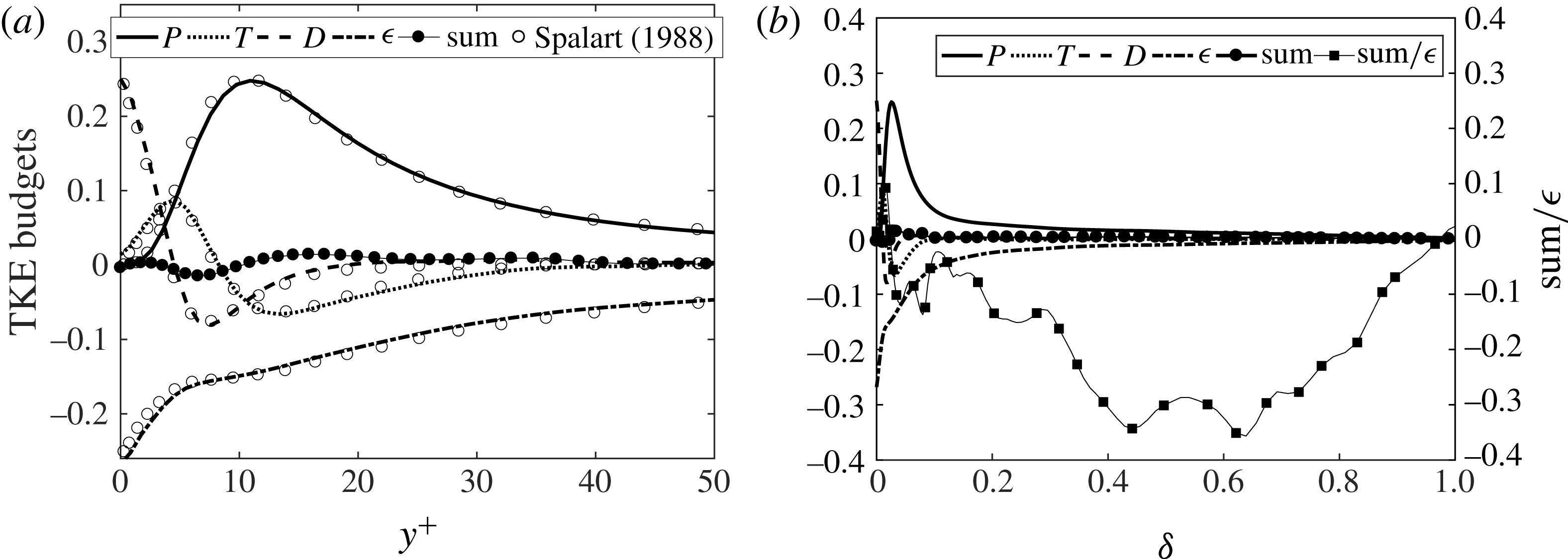
Figure 4 shows the turbulent kinetic energy budget in different wall distance scales. Here all the terms are normalized by
 $u_{\unicode[STIX]{x1D70F}}^{4}/\unicode[STIX]{x1D708}$
. Basically the production and the dissipation terms are the dominant parts, except in the vicinity of the wall, where turbulent transport and viscous diffusion become important. It can be seen that the sum of budget terms does not entirely vanish. In the near-wall region, the relative sum error
 $\text{sum}/\unicode[STIX]{x1D716}$
(compared with the dissipation term) is small. Far away from the wall,
 $\unicode[STIX]{x1D716}$
is smaller and the absolute value of the relative error is larger, which may be attributed to the relatively short statistical averaging time in the far-wall region. However, tests in the Appendix justify that the statistical averaging time is sufficiently long for satisfactory statistical convergence of quantities relevant for the analysis in the following sections.
Turbulent kinetic energy budget relation (normalized by
 $u_{\unicode[STIX]{x1D70F}}^{4}/\unicode[STIX]{x1D708}$
): (a) for the range
 $0\leqslant y^{+}\leqslant 50$
; (b) for the entire boundary layer region with the sum error.

3 Vectorline segment analysis
Vectorline segment analysis is implemented to investigate the intrinsic topology of the turbulent boundary layer. In a turbulent vector field
 $\boldsymbol{v}$
with magnitude
 $v=|\boldsymbol{v}|$
, except for the singular points, which are defined as the points with zero
 $v$
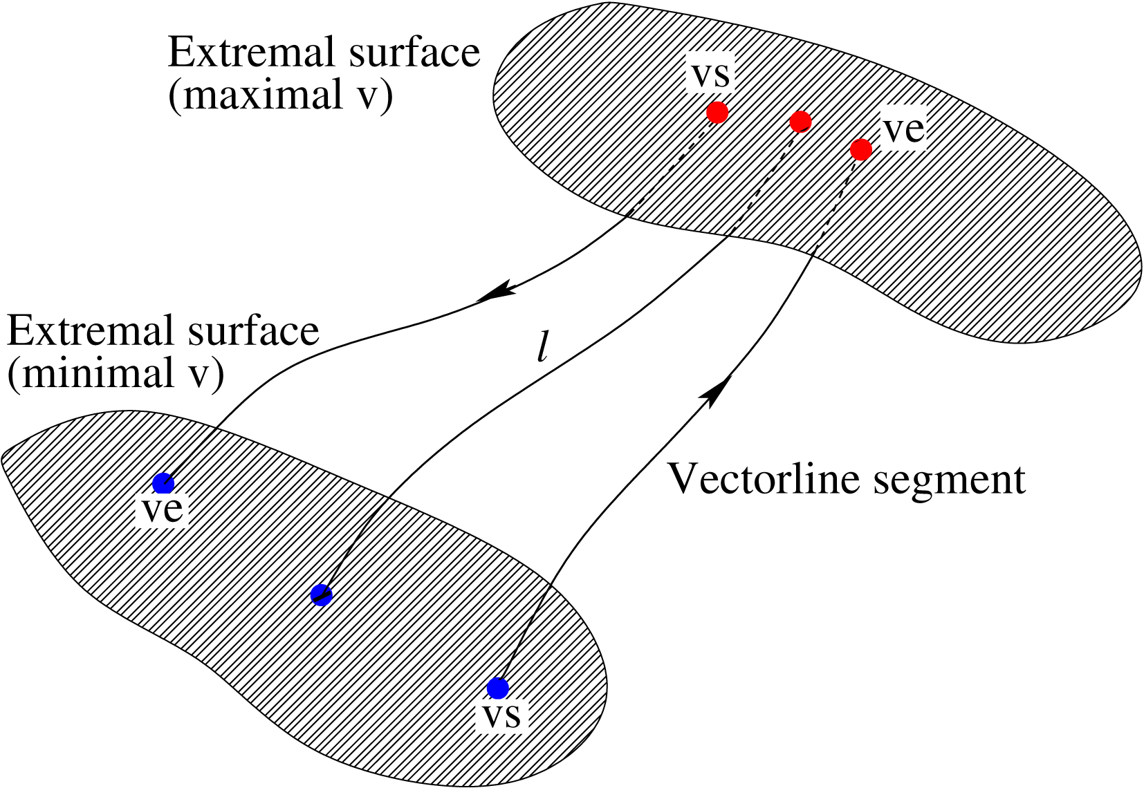
, the vector direction is uniquely determined. The vectorline, locally tangent to the vector under consideration, is named ‘streamline’ for the velocity vector case and ‘vorticity line’ for the vorticity vector case, respectively. Figure 5 illustrates the schematic of the vectorline segment structure. As introduced by Wang (Reference Wang2010), starting from any non-singular point, along either the vector direction or the inverse direction, one will reach a local extremum of
 $v$
. The part of the vectorline between the two local extrema of
 $v$
is defined as a vectorline segment, belonging to the given spatial point. Therefore, within a vectorline segment
 $v$
changes monotonically from
 $v_{s}$
at one end to
 $v_{e}$
at the other end along the vector direction. The arclength
 $l$
of the segment and
 $\unicode[STIX]{x0394}v=v_{e}-v_{s}$
are chosen as the characteristic parameters to describe the vectorline segment structure. According to the sign of
 $\unicode[STIX]{x0394}v$
, a vectorline segment can be either positive (if
 $\unicode[STIX]{x0394}v$
is positive) or negative (if
 $\unicode[STIX]{x0394}v$
is negative). In principle, the geometrical statistics of vectorline segments inherit important physics of the turbulent field. It is worth mentioning that, although the vectorline segments are undermined at singular points, whose volume portion is, however, negligibly small, the statistical results will not be influenced.
Schematic of the vectorline segment structure. From any non-singular point following the vectorline, along either the vector direction or its inverse, one will reach a local extremum of the vector magnitude
 $v$
. The part of the vectorline between the two local extrema is defined as the vectorline segment corresponding to this spatial point. A segment can be either positive or negative if
 $v$
increases or decrease along
 $\boldsymbol{v}$
.

4 Results and discussion
Velocity and vorticity, two vectors of primary importance in fluid dynamics, will be analysed. The characteristic parameters, which are the arclength and vector magnitude difference, are denoted as
 $l_{u}$
and
 $\unicode[STIX]{x0394}u$
for streamline segments and
 $l_{\unicode[STIX]{x1D714}}$
and
 $\unicode[STIX]{x0394}\unicode[STIX]{x1D714}$
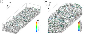
for vorticity line segments. Note that the segments are defined based on the complete quantities, i.e. the complete velocity and complete vorticity, instead of the fluctuating ones. Figure 6 plots both the vorticity lines and vortex tubes from a field snapshot. Very probably the orientations of both entities are aligned, indicating some geometrical features in common. Meanwhile, when moving away from the wall, on average the vorticity strength decreases and correspondingly the vortex tubes become larger.
The spatial structure of vorticity lines and the vortex tubes (obtained from isosurfaces of the second invariant
 $Q$
of the velocity gradient): (a) an overall view, and (b) a local view. On average the magnitude of vorticity increases as the wall distance decreases.

Numerically, to remove the unphysical influence from the domain boundaries, a sub-zone is selected for analysis to ensure the flow (quasi-)homogeneity in the streamwise and spanwise directions. Specifically, the sub-zone size along
 $x$
,
 $y$
and
 $z$
are
 $7\unicode[STIX]{x1D6FF}_{in}$
,
 $1.4\unicode[STIX]{x1D6FF}_{in}$
and
 $\unicode[STIX]{x1D6FF}_{in}$
, respectively, i.e. from the entire domain
 $2\unicode[STIX]{x1D6FF}_{in}$
upstream cut,
 $2\unicode[STIX]{x1D6FF}_{in}$
downstream cut, and
 $0.5\unicode[STIX]{x1D6FF}_{in}$
cut on both span sides. All the grid points in the sub-zone are used to trace the corresponding vectorline segments. In the present analysis, because of inhomogeneity in the wall-normal direction, vectorline segments corresponding to the grid points at specified wall-normal distances are sampled for statistics.
4.1 Segment length statistics
4.1.1 The mean segment length
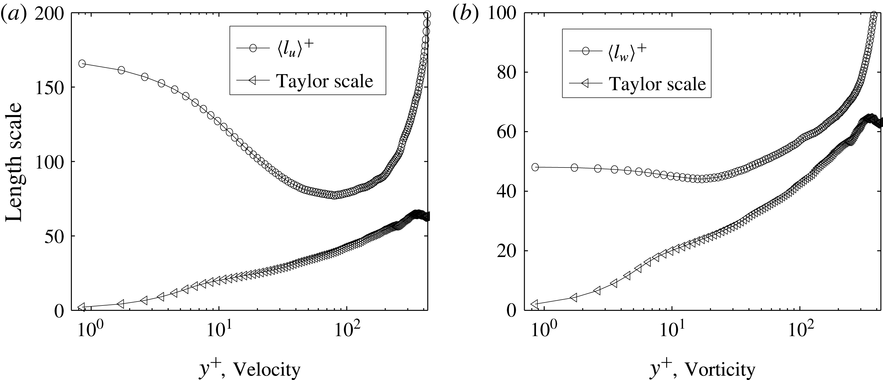
The mean length of vectorline segments quantifies the scale of the local structure. Figure 7 shows for both vectors the dependence of the segment mean length on the wall-normal distance
 $y^{+}$
, where the superscript
 $+$
denotes normalization by the viscous unit. Meanwhile, the Taylor scale, which for boundary layer turbulence is defined as
 $\unicode[STIX]{x1D706}(y^{+})=\sqrt{10\unicode[STIX]{x1D708}k(y^{+})/\unicode[STIX]{x1D716}(y^{+})}$
, is also plotted for comparison. Here
 $k(y^{+})$
and
 $\unicode[STIX]{x1D716}(y^{+})$
are the averaged turbulent kinetic energy and the averaged energy dissipation conditioned at specified
 $y^{+}$
, respectively. For streamline segments, the mean length
 $\langle l_{u}\rangle ^{+}$
decreases quickly in the viscous sublayer (
 $y^{+}<10$
) and buffer layer (
 $10<y^{+}<30$
), and reaches its minimum in the log-law region at approximately
 $y^{+}\approx 80$
. Afterwards
 $\langle l_{u}\rangle ^{+}$
increases more and more rapidly until the edge of the boundary layer. For vorticity line segments in the viscous sublayer and part of the buffer layer, the mean length
 $\langle l_{\unicode[STIX]{x1D714}}\rangle ^{+}$
decreases slowly and then starts to increase in the entire log-law region and beyond.
The variation of (a)
 $\langle l_{u}\rangle$
for the streamline segments and (b)
 $\langle l_{\unicode[STIX]{x1D714}}\rangle$
for the vorticity line segments, as a function of
 $y^{+}$
.

Physically, the mean length is dominated by the scale of the local flow structure and the perturbation strength, which can roughly be understood as the local turbulence intensity. On the one hand, the flow structure, for instance shown in figure 1, evolves to be larger from the wall boundary towards the outside, making the segments longer. On the other hand, stronger perturbation, as well as larger turbulence intensity, tends to disturb the flow field to generate more extremal points, making the segments shorter. Within the viscous sublayer, the turbulent intensity increases and then continues to decrease from the buffer region. Therefore the mean length of both the streamline segments and vorticity line segments decreases first and then increases. Overall, for vorticity line segments, the mean length
 $\langle l_{\unicode[STIX]{x1D714}}\rangle ^{+}$
is much smaller than
 $\langle l_{u}\rangle ^{+}$
. A sharp difference is that from the solid wall surface
 $\langle l_{u}\rangle ^{+}$
decreases largely till
 $y^{+}\approx 80$
, while
 $\langle l_{\unicode[STIX]{x1D714}}\rangle ^{+}$
decreases weakly in a much shorter range till
 $y^{+}=20$
, which may be an indication that the vorticity line segments are more influenced by the flow structure than turbulence perturbation.
4.1.2 Probability density function of the length distribution
More detailed information on the segment length can be viewed from its probability density function (p.d.f.). Work has been done in studying the scale of dissipation elements (Wang & Peters Reference Wang and Peters2006, Reference Wang and Peters2008). Physically, the segment length
 $l$
is determined by the generation and annihilation of extremal points. On the one hand, turbulent random motion disturbs the flow to generate new extremal points. On the other hand, viscous diffusion annihilates the closely located extremal points to smoothen the flow field. Besides these two abrupt effects, there is another drift velocity representing the continuous change of
 $l$
. In a general scenario, the evolution of
 $l$
can be modelled based on a Poisson random cutting–reconnection process. Considering one-dimensional space, each segment is bounded by two extremal points, and all the segments are connected with each other to fill the entire space. Once a newly generated extremal point is added into a segment, it is then cut into two smaller segments. Meanwhile, if two adjacent extremal points merge and then annihilate because of viscous diffusion, two smaller segments can connect to generate a large one. In total, the birth and death of segments are summarized as the following mechanism:
(i) generation by cutting (
 $GC$
);
(ii) generation by reconnection (
$GR$
);(iii) removal by cutting (
$RC$
);(iv) removal by reconnection (
$RR$
).


Collecting all the above contributions, together with the drift velocity, one obtains the following equation for the p.d.f. of the segment length
 $l$
as (Wang & Peters Reference Wang and Peters2006, Reference Wang and Peters2008):
 $$\begin{eqnarray}\displaystyle \frac{\unicode[STIX]{x2202}P(l,t)}{\unicode[STIX]{x2202}t}+\frac{\unicode[STIX]{x2202}(v(l)P(l,t))}{\unicode[STIX]{x2202}l} & = & \displaystyle \int _{0}^{\infty }2\unicode[STIX]{x1D706}P(l+z)\,\text{d}z-\unicode[STIX]{x1D706}lP(l,t)\nonumber\\ \displaystyle & & \displaystyle \times \,\int _{0}^{l}2\unicode[STIX]{x1D707}\frac{z}{l}P(l-z)P(z)\,\text{d}z-2\unicode[STIX]{x1D707}P(l,t).\end{eqnarray}$$
Here
 $v(l)$
is the drift velocity at scale
 $l$
,
 $\unicode[STIX]{x1D706}$
is the cutting frequency per unit length, and
 $\unicode[STIX]{x1D707}$
is the disappearance rate of extreme points, which can be determined as
 $\unicode[STIX]{x1D707}=4D(\unicode[STIX]{x2202}P(x,t)/\unicode[STIX]{x2202}x)|_{x=0}$
, where
 $D$
is the fluid viscosity. The four terms on the right-hand side represent
 $GC$
,
 $RC$
,
 $GR$
and
 $RR$
, respectively. In the non-dimensional form, the p.d.f. of
 $\tilde{l}=l/\langle l\rangle$
, i.e. the length scale normalized by its mean
 $\langle l\rangle$
, becomes
 $$\begin{eqnarray}\displaystyle \frac{\unicode[STIX]{x2202}P(\tilde{l},t)}{\unicode[STIX]{x2202}t}+\frac{\unicode[STIX]{x2202}}{\unicode[STIX]{x2202}\tilde{l}}(\tilde{v}(\tilde{l})P(\tilde{l},t)) & = & \displaystyle \unicode[STIX]{x1D6EC}\left[\int _{0}^{\infty }2P(\tilde{l}+\tilde{z},t)\,\text{d}\tilde{z}-\tilde{l}P(\tilde{l},t)\right]\nonumber\\ \displaystyle & & \displaystyle \left.+\,8\frac{\unicode[STIX]{x2202}P(\tilde{l},t)}{\unicode[STIX]{x2202}\tilde{l}}\right|_{\tilde{l}=0}\left[\int _{0}^{\tilde{l}}\frac{\tilde{z}}{\tilde{l}}P(\tilde{l}-\tilde{z},t)P(\tilde{z},t)\,\text{d}\tilde{z}-P(\tilde{l},t)\right].\nonumber\\ \displaystyle & & \displaystyle\end{eqnarray}$$
Here
 $\unicode[STIX]{x1D6EC}$
is an eigenvalue, which can be determined from the p.d.f.’s normalization condition. At the statistically stationary state, there is a dynamic balance under the action of all these mechanisms and the p.d.f. equation (4.2) has a unique time-independent solution. Results from different problems such as the dissipation element scale in passive scalar turbulence (Wang & Peters Reference Wang and Peters2006), the scale distribution in Lagrangian turbulence (Wang Reference Wang2014) and reactive turbulence (Wang, Chakraborty & Zhang Reference Wang, Chakraborty and Zhang2013) justify that such a solution is applicable with good generality.
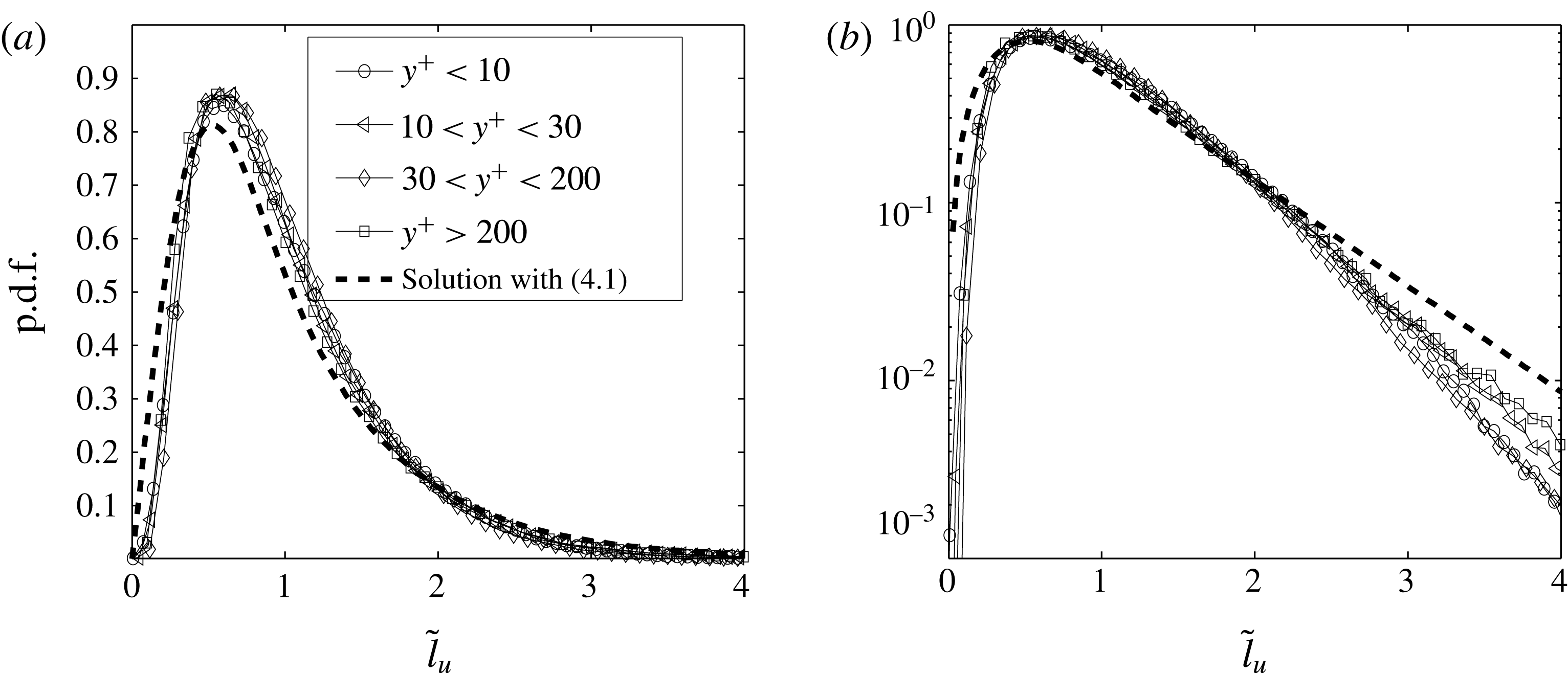
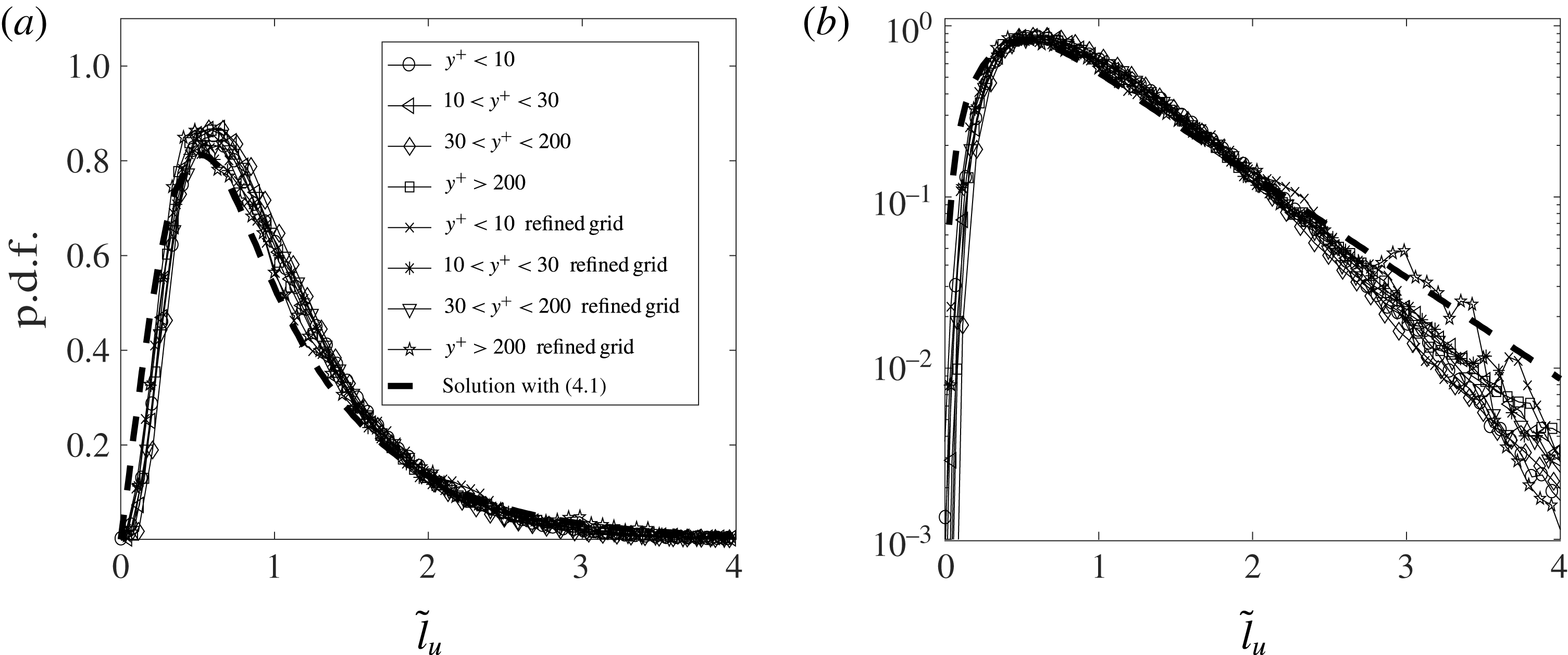
Figure 8 shows the p.d.f. of streamline segment length
 $\tilde{l}_{u}$
at different wall-normal distances, in both linear–linear and log–linear coordinates. Compared with the stationary solution of (4.2), the agreement is satisfactory, which implies that the aforementioned smoothing mechanism, the random perturbation mechanism and the continuous drift are generally valid in describing the streamline segment behaviour. It is noteworthy that in the log–linear plot, the p.d.f.’s exponential tail can be explained by a Poisson-like process at the large scale in deriving (4.2).
P.d.f. of
 $\tilde{l}_{u}=l_{u}/\langle l_{u}\rangle$
compared with the solution of (4.2) in (a) linear–linear coordinates and (b) log–linear coordinates.

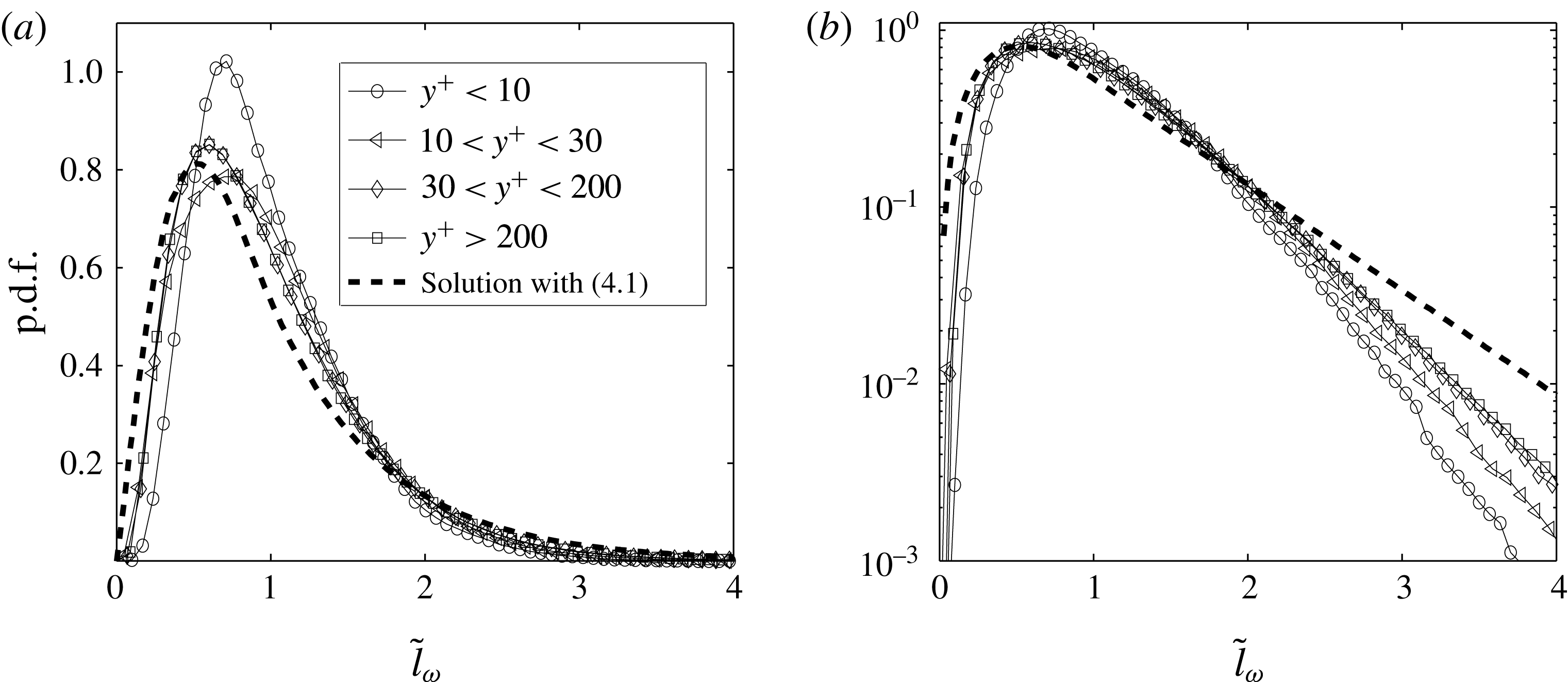
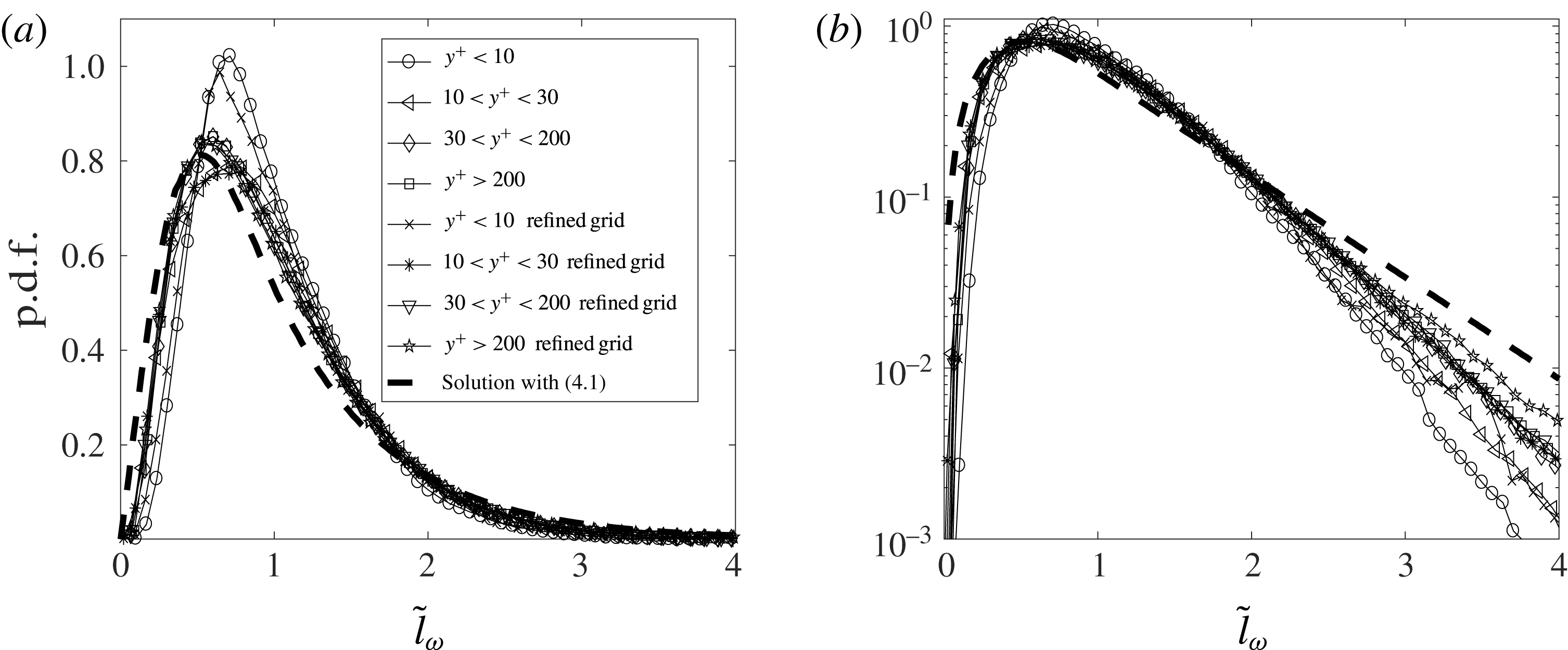
For vorticity line segments, the length p.d.f. is shown in figure 9, in both linear–linear and log–linear coordinates. Differently from the
 $\tilde{l}_{u}$
case, the
 $\text{p.d.f.}(\tilde{l}_{\unicode[STIX]{x1D714}})$
at different
 $y^{+}$
is not universal. At larger
 $y^{+}$
(for instance, when
 $y^{+}>30$
) the numerical result matches the solution of (4.2); however, when closer to the wall, the numerical result deviates more from the equation solution. A tentative explanation of such an outcome is that the strong shear stress near the solid wall may invalidate the smoothing and random perturbation mechanisms in deriving (4.2).
P.d.f. of
 $\tilde{l}_{\unicode[STIX]{x1D714}}=l_{\unicode[STIX]{x1D714}}/\langle l_{\unicode[STIX]{x1D714}}\rangle$
compared with the solution of (4.2) in (a) linear–linear coordinates and (b) log–linear coordinates.

4.2 Joint p.d.f. between the characteristic parameters
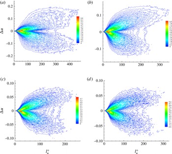
Besides the segment length p.d.f., the joint p.d.f. between the characteristic parameters is more informative. Figure 10 shows such joint p.d.f.s for streamline segments corresponding to grid points at four different wall-normal distances, i.e.
 $y^{+}=2.6$
,
 $y^{+}=20$
,
 $y^{+}=80$
and
 $y^{+}=275$
, which according to the mean velocity profile in figure 2 represent the typical samples in the viscous sublayer, buffer layer, log-law region and outer layer, respectively. Here
 $\unicode[STIX]{x0394}u$
is non-dimensionalized by the speed of sound. Each joint p.d.f. has two branches, one with positive
 $\unicode[STIX]{x0394}u$
and the other with negative
 $\unicode[STIX]{x0394}u$
. Interestingly, in the viscous sublayer, these two branches are almost symmetrical. When moving to the buffer layer, the positive branch becomes clearly larger, whereas in the log-law region and outer layer such asymmetry weakens again and finally almost disappears.
Joint p.d.f. of
 $l_{u}$
and
 $\unicode[STIX]{x0394}u$
at different wall-normal distances: (a)
 $y^{+}=2.6$
(in the viscous sublayer); (b)
 $y^{+}=20$
(in the buffer layer); (c)
 $y^{+}=80$
(in the log-law region); and (d)
 $y^{+}=275$
(in the outer layer).

Because of the monotonic change of
 $u$
along the streamline segments,
 $\unicode[STIX]{x0394}u/l_{u}$
can be interpreted as a kind of averaged velocity derivative. Therefore the asymmetry of the joint p.d.f. implies the unequal contributions from the positive and negative velocity derivative parts in the flow field, which can be approximately quantified by the skewness of the velocity derivative. For the present boundary layer flow, streamline segments are most probably aligned along the streamwise direction. Therefore it is meaningful to investigate the skewness of the streamwise velocity component derivative, i.e.
 $$\begin{eqnarray}S=\langle (\text{d}u_{1}/\text{d}x)^{3}\rangle /\langle (\text{d}u_{1}/\text{d}x)^{2}\rangle ^{3/2}.\end{eqnarray}$$
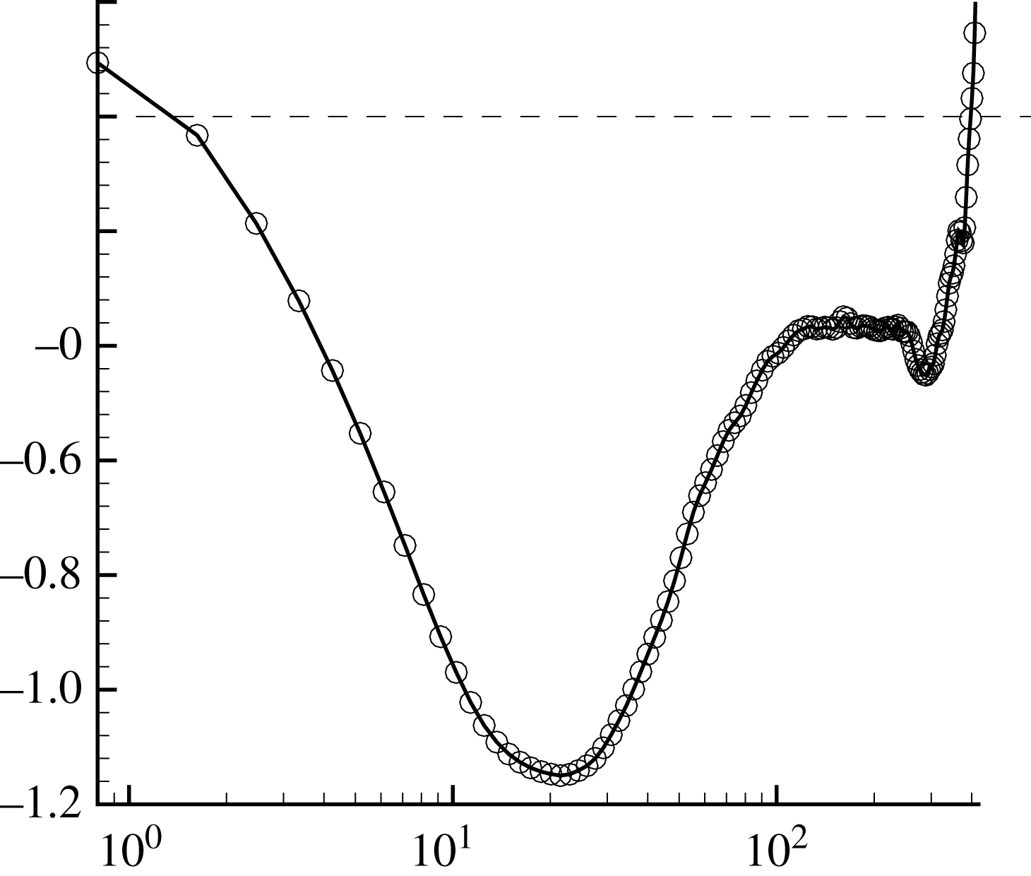
As demonstrated in figure 11, in most of the boundary layer region, the skewness is negative. Around
 $y^{+}=20$
,
 $S$
reaches its minimum and then increases. A similar behaviour has been observed by Vreman & Kuerten (Reference Vreman and Kuerten2014). As
 $y^{+}$
varies, the change of skewness in figure 11 conforms with the change of the joint p.d.f. asymmetry.
Dependence of the skewness of the streamwise velocity component derivative on the wall-normal distance. In coincidence with the asymmetry of the joint p.d.f.s in figure 10, the skewness reaches a minimum in the buffer layer.

Physically, the negative skewness of the velocity derivative represents the average rate of vorticity production through vortex stretching (Taylor Reference Taylor1938; Monin & Yaglom Reference Monin and Yaglom2007). Vreman & Kuerten (Reference Vreman and Kuerten2014) believed that the negative peak is caused by local coherent structures. In the context of streamline segment analysis, the negative skewness can be interpreted from the joint p.d.f. of
 $l_{u}$
and
 $\unicode[STIX]{x0394}u$
. As has been extensively studied (Wang Reference Wang2010; Boschung et al.
Reference Boschung, Schaefer, Peters and Meneveau2014), the asymmetry of the joint p.d.f. is one of the most important results from streamline segment statistics in isotropic turbulence. Considering an individual streamline segment, the velocity magnitude
 $u$
along the vector direction will increase monotonically if the segment is positive, or decrease if the segment is negative. Therefore, when evolving with time, positive segments with increasing
 $u$
tend to be elongated, while negative segments tend to be compressed because of decreasing
 $u$
along the vector direction. Consequently, on average, the cube of the negative derivative becomes larger, while the cube of the positive derivative becomes smaller, resulting in negative
 $S$
.
From the joint p.d.f., the conditional mean
 $\unicode[STIX]{x0394}u$
can be defined as
 $\langle \unicode[STIX]{x0394}u\rangle =\int \!\unicode[STIX]{x0394}uP(\unicode[STIX]{x0394}u,l_{u})\,\text{d}\unicode[STIX]{x0394}u$
. To differentiate the positive and negative branches,
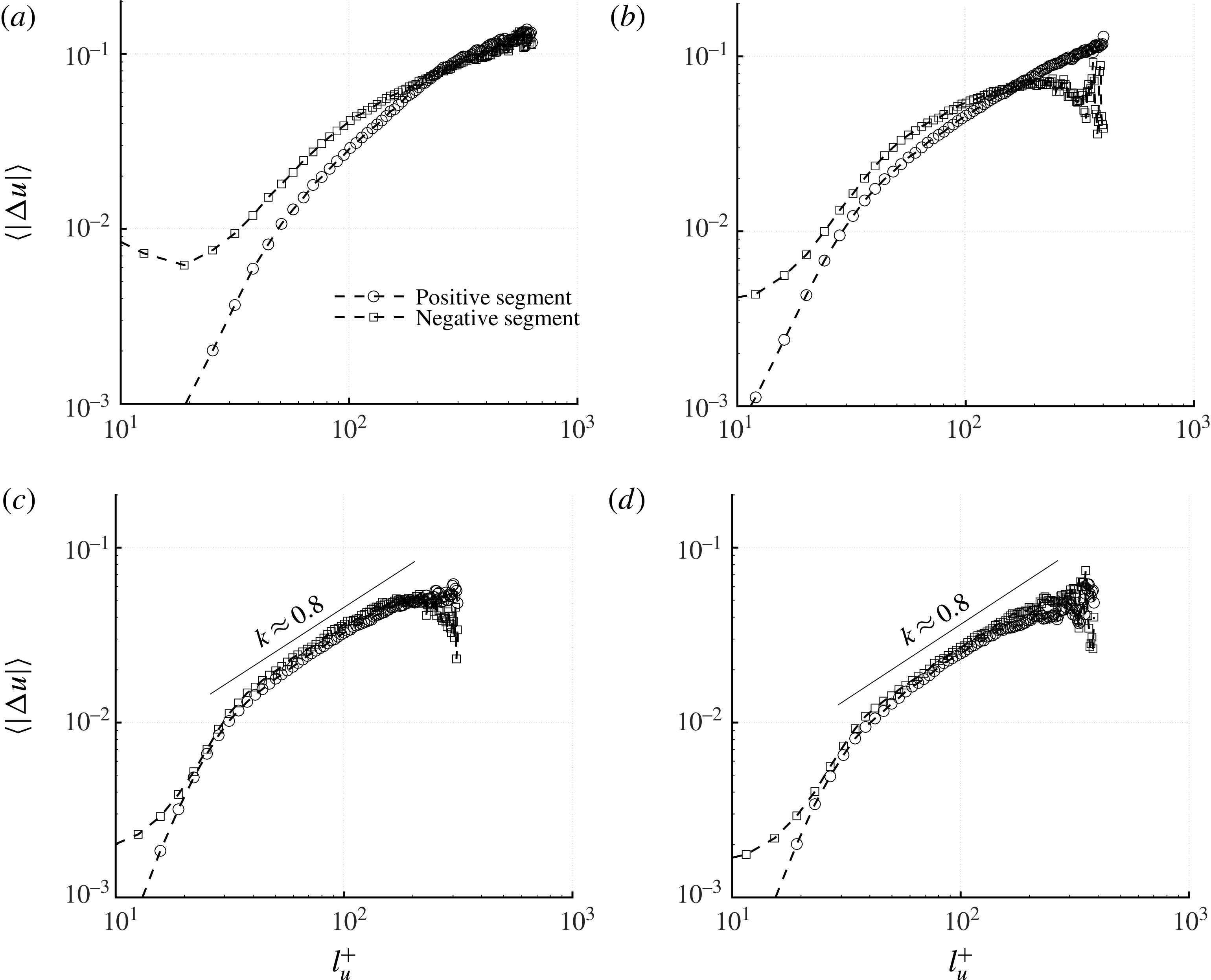
 $\langle |\unicode[STIX]{x0394}u|\rangle =\int \!|\unicode[STIX]{x0394}u|P(\unicode[STIX]{x0394}u,l_{u})\,\text{d}\unicode[STIX]{x0394}u$
are calculated separately for positive segments and negative segments. The results are shown in figure 12. In the log-law region and the outer layer,
 $\langle |\unicode[STIX]{x0394}u|\rangle$
from the positive and negative segments are almost identical for
 $l_{u}>20$
, with a scaling exponent approximately 0.8. Differently, in the viscous and buffer sublayers, the positive and negative segments have different conditional mean
 $\langle |\unicode[STIX]{x0394}u|\rangle$
and there is no clear scaling behaviour. Especially in the smaller
 $l_{u}$
range,
 $\langle |\unicode[STIX]{x0394}u|\rangle$
from the positive segments is smaller, while in the larger
 $l_{u}$
range,
 $\langle |\unicode[STIX]{x0394}u|\rangle$
from the negative segments is smaller.
The conditional mean of
 $|\unicode[STIX]{x0394}u|$
, calculated separately for the positive and negative segments, at different wall-normal distances corresponding to figure 10: (a)
 $y^{+}=2.6$
(in the viscous sublayer); (b)
 $y^{+}=20$
(in the buffer layer); (c)
 $y^{+}=80$
(in the log-law region); and (d)
 $y^{+}=275$
(in the outer layer).

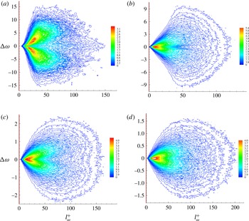
For vorticity line segments, the joint p.d.f.s between
 $l_{\unicode[STIX]{x1D714}}$
and
 $\unicode[STIX]{x0394}\unicode[STIX]{x1D714}$
at different
 $y^{+}$
are shown in figure 13. Here
 $\unicode[STIX]{x0394}\unicode[STIX]{x1D714}$
is non-dimensionalized by the speed of sound and the boundary layer thickness. Compared with figure 10, a clear difference is that the positive
 $\unicode[STIX]{x0394}\unicode[STIX]{x1D714}$
and negative
 $\unicode[STIX]{x0394}\unicode[STIX]{x1D714}$
branches are symmetric throughout the boundary layer. The reason is that, for vorticity line segments, the aforementioned kinematic mechanism, leading on average to longer positive streamline segments and shorter negative streamline segments, does not exist (Wang Reference Wang2012). The positive
 $\unicode[STIX]{x0394}\unicode[STIX]{x1D714}$
and negative
 $\unicode[STIX]{x0394}\unicode[STIX]{x1D714}$
branches are well separated in the viscous sublayer, and then become closer when
 $y^{+}$
increases. Moreover, at larger
 $y^{+}$
,
 $\unicode[STIX]{x0394}\unicode[STIX]{x1D714}$
decreases because of smaller velocity gradient and thus vorticity.
Joint p.d.f. of
 $l_{\unicode[STIX]{x1D714}}$
and
 $\unicode[STIX]{x0394}\unicode[STIX]{x1D714}$
at different wall-normal distances: (a)
 $y^{+}=2.6$
(in the viscous sublayer); (b)
 $y^{+}=20$
(in the buffer layer); (c)
 $y^{+}=80$
(in the log-law region); and (d)
 $y^{+}=275$
(in the outer layer).

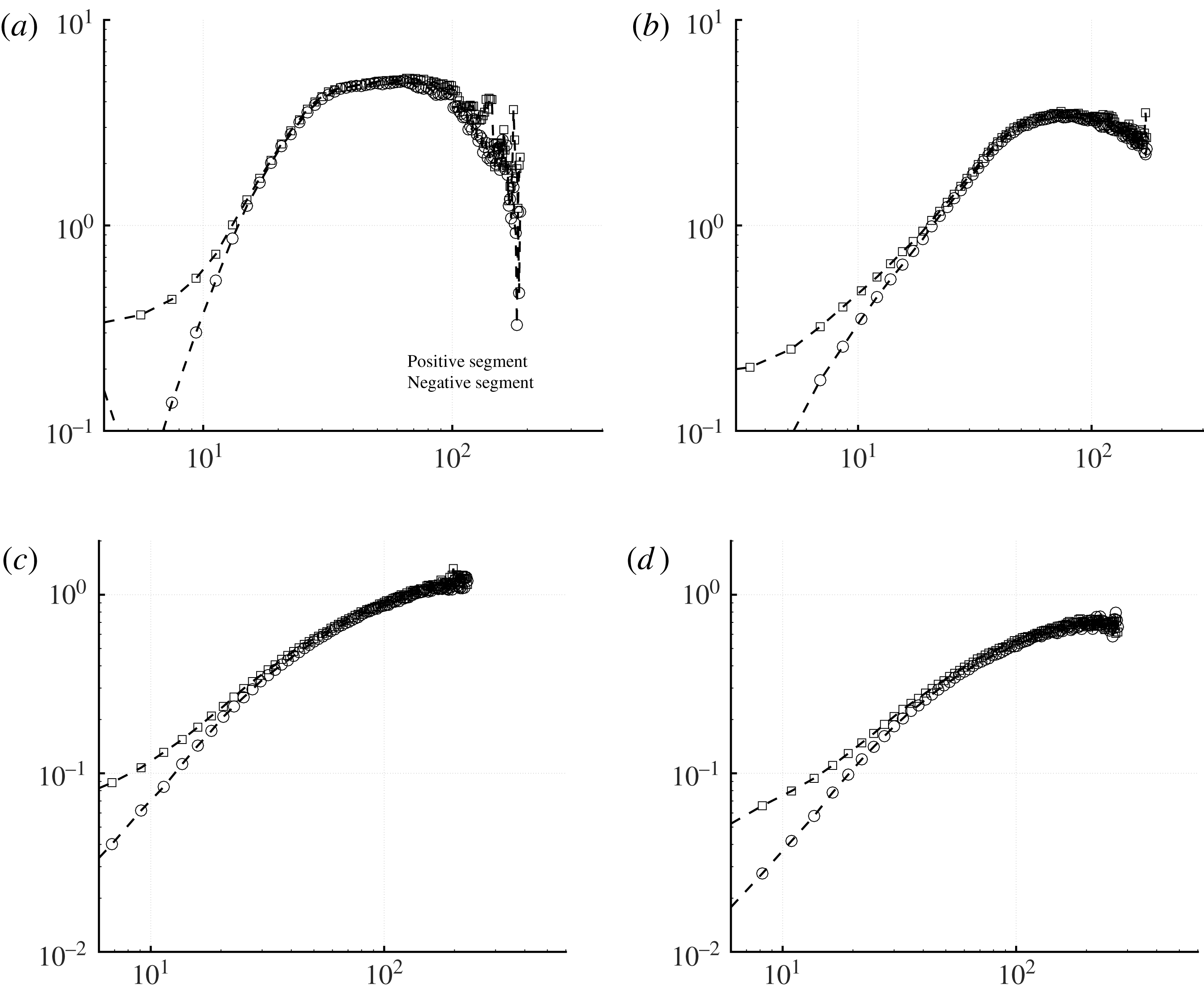
Figure 14 plots the conditional mean of
 $|\unicode[STIX]{x0394}\unicode[STIX]{x1D714}|$
as a function of
 $l_{\unicode[STIX]{x1D714}}$
, which is almost identical for the positive and negative segments. In different boundary layer regions, no obvious scaling can be observed. Especially in the viscous sublayer and buffer layer,
 $\langle |\unicode[STIX]{x0394}\unicode[STIX]{x1D714}|\rangle$
levels off and then drops down at larger
 $l_{\unicode[STIX]{x1D714}}$
.
The conditional mean of
 $|\unicode[STIX]{x0394}\unicode[STIX]{x1D714}|$
, calculated separately for the positive and negative vorticity line segments, at different wall-normal distances corresponding to figure 10: (a)
 $y^{+}=2.6$
(in the viscous sublayer); (b)
 $y^{+}=20$
(in the buffer layer); (c)
 $y^{+}=80$
(in the log-law region); and (d)
 $y^{+}=275$
(in the outer layer).

4.3 The segment spatial structure
We denote the Cartesian coordinate differences between the segment starting point
 $s$
and ending point
 $e$
as
 $\unicode[STIX]{x0394}x=x_{e}-x_{s}$
,
 $\unicode[STIX]{x0394}y=y_{e}-y_{s}$
and
 $\unicode[STIX]{x0394}z=z_{e}-z_{s}$
. In isotropic turbulence without any preference of spatial orientation of the segments,
 $\unicode[STIX]{x0394}x$
,
 $\unicode[STIX]{x0394}y$
and
 $\unicode[STIX]{x0394}z$
need to be uncorrelated. Therefore, the anisotropy of the turbulent boundary layer can be characterized via the segment orientation statistics.
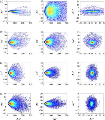
For streamline segments, the correlations between
 $\unicode[STIX]{x0394}x$
,
 $\unicode[STIX]{x0394}y$
and
 $\unicode[STIX]{x0394}z$
, or between
 $\unicode[STIX]{x0394}x^{+}$
,
 $\unicode[STIX]{x0394}y^{+}$
and
 $\unicode[STIX]{x0394}z^{+}$
in the normalized form, are shown in figure 15. The main findings are summarized as follows.
(i) Because of the dominant velocity component along the streamwise direction, segments tend to align with
$x$
. Therefore
$\unicode[STIX]{x0394}x^{+}$
is very probably positive and the magnitude of
$\unicode[STIX]{x0394}x^{+}$
is much larger than that of
$\unicode[STIX]{x0394}y^{+}$
and
$\unicode[STIX]{x0394}z^{+}$
, as shown in the joint p.d.f.s between
$\unicode[STIX]{x0394}x^{+}$
and
$\unicode[STIX]{x0394}y^{+}$
, and between
$\unicode[STIX]{x0394}x^{+}$
and
$\unicode[STIX]{x0394}z^{+}$
. As
$y^{+}$
increases, on average
$\unicode[STIX]{x0394}x^{+}$
first decreases and then increases, which can be explained from the variation of the mean segment length, as shown in figure 7.(ii) For the joint p.d.f.s between
$\unicode[STIX]{x0394}x^{+}$
and
$\unicode[STIX]{x0394}y^{+}$
, in the near vicinity of the wall, e.g.
$y^{+}=2.6$
, because of the boundary confinement, the streamline segments are forced to bend up, and thus
$\unicode[STIX]{x0394}y^{+}$
is probably positive. When moving to the buffer layer at
$y^{+}=20$
, the positive
$\unicode[STIX]{x0394}y^{+}$
part becomes larger. Such an observation indicates that the sweep events in the ‘bursting cycle’ (Kline et al.
Reference Kline, Reynolds, Schraub and Runstadler1967) predominate the production and regeneration of near-wall turbulence, which is consistent with quadrant analysis (Wallace Reference Wallace2016). From the buffer layer to the outer layer, the segments then gradually bend down with negative
$\unicode[STIX]{x0394}y^{+}$
. Especially at large
$y^{+}$
as
$y^{+}=275$
, the negative
$\unicode[STIX]{x0394}y^{+}$
part can be clearly observed.(iii) The joint p.d.f.s between
$\unicode[STIX]{x0394}y^{+}$
and
$\unicode[STIX]{x0394}z^{+}$
demonstrate that at
$y^{+}=2.6$
on average the magnitude of
$\unicode[STIX]{x0394}z^{+}$
is much larger than that of
$\unicode[STIX]{x0394}y^{+}$
, which means that the streamline segments are more likely to swing along the spanwise direction than the wall-normal direction. A possible explanation is that the internal shear layers (or vorticity sheets) dominate the dynamic behaviour of the near-wall streaks (Schoppa & Hussain Reference Schoppa and Hussain2002). With the increase of
$y^{+}$
, the magnitude of
$\unicode[STIX]{x0394}z^{+}$
shrinks gradually and
$\unicode[STIX]{x0394}y^{+}$
and
$\unicode[STIX]{x0394}z^{+}$
are comparable. Such a tendency agrees with the change of the turbulence kinetic energy of each velocity component. In principle,
$\unicode[STIX]{x0394}y^{+}$
and
$\unicode[STIX]{x0394}z^{+}$
are closely related to the velocity fluctuations along the
$y$
and
$z$
directions, or equivalently to
$\langle u_{2}^{\prime 2}\rangle$
and
$\langle u_{3}^{\prime 2}\rangle$
, respectively. For
$y^{+}$
as small as
$y^{+}=2.6$
,
$\langle u_{3}^{\prime 2}\rangle$
is much larger than
$\langle u_{2}^{\prime 2}\rangle$
, while for larger
$y^{+}$
,
$\langle u_{3}^{\prime 2}\rangle$
and
$\langle u_{2}^{\prime 2}\rangle$
become closer.


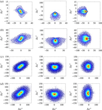
For vorticity line segments, the main results are presented in figure 16 with the following findings.
- (iv)
The joint p.d.f.s between
$\unicode[STIX]{x0394}x^{+}$
and
$\unicode[STIX]{x0394}y^{+}$
suggest that the magnitudes of
$\unicode[STIX]{x0394}x^{+}$
and
$\unicode[STIX]{x0394}y^{+}$
are comparable. At different
$y^{+}$
, the positive
$\unicode[STIX]{x0394}y^{+}$
part and the negative
$\unicode[STIX]{x0394}y^{+}$
part are almost symmetric. When
$y^{+}$
increases, on average the magnitudes of
$\unicode[STIX]{x0394}y^{+}$
and
$\unicode[STIX]{x0394}x^{+}$
increase, because of the larger turbulent structure. At
$y^{+}=2.6$
,
$\unicode[STIX]{x0394}x^{+}$
and
$\unicode[STIX]{x0394}y^{+}$
are negatively correlated, while moving away from the wall such correlation becomes positive and
$\unicode[STIX]{x0394}x^{+}$
on average is marginally larger than
$\unicode[STIX]{x0394}y^{+}$
. The two peaks of the joint p.d.f. may be closely related to the hairpin vortex structure and the orientation of the maximum strain rate (Head & Bandyopadhyay Reference Head and Bandyopadhyay1981). Further quantitative investigation is needed to better understand the segment statistics.- (v)
From the joint p.d.f.s between
$\unicode[STIX]{x0394}x^{+}$
and
$\unicode[STIX]{x0394}z^{+}$
and between
$\unicode[STIX]{x0394}z^{+}$
and
$\unicode[STIX]{x0394}y^{+}$
, we see that at
$y^{+}=2.6$
, because of the large shear strain rate and thus the vorticity magnitude, the segments are typically oriented in the
$z$
direction and
$\unicode[STIX]{x0394}z^{+}$
is very probably negative. When
$y^{+}$
increases, the positive
$\unicode[STIX]{x0394}z^{+}$
part becomes larger because of the stronger perturbation from turbulent eddies, while the negative part remains almost invariant. Overall the negative part is larger. In the log-law region and the outer layer,
$\unicode[STIX]{x0394}x^{+}$
,
$\unicode[STIX]{x0394}y^{+}$
and
$\unicode[STIX]{x0394}z^{+}$
are all comparable in magnitude.- (vi)
The joint p.d.f.s between
$\unicode[STIX]{x0394}y^{+}$
and
$\unicode[STIX]{x0394}z^{+}$
are symmetric across the abscissa axis, which means that vorticity line segments have no preference to bend upwards or downwards. When
$y^{+}$
increases, the positive and negative
$\unicode[STIX]{x0394}y^{+}$
branches become less separated because the flow is more isotropic.


For the streamline segments, the joint p.d.f. between the spatial coordinates (
 $\unicode[STIX]{x0394}x$
,
 $\unicode[STIX]{x0394}y$
and
 $\unicode[STIX]{x0394}z$
) at (a)
 $y^{+}=2.6$
, (b)
 $y^{+}=20$
, (c)
 $y^{+}=80$
and (d)
 $y^{+}=275$
.

For the vorticity line segments, the joint p.d.f. between the spatial coordinates (
 $\unicode[STIX]{x0394}x$
,
 $\unicode[STIX]{x0394}y$
and
 $\unicode[STIX]{x0394}z$
) at (a)
 $y^{+}=2.6$
, (b)
 $y^{+}=20$
, (c)
 $y^{+}=80$
and (d)
 $y^{+}=275$
.

Resolution independence check for the p.d.f. of
 $\tilde{l}_{u}=l_{u}/\langle l_{u}\rangle$
.

5 Conclusions
The velocity and vorticity vector fields of a zero-pressure-gradient turbulent boundary layer flow have been investigated based on vectorline segment analysis. For a specified vector field, the vectorline, a structure independent of the reference frame, inherits important flow characteristics. From any non-singular point, along either the vector or the inverse direction, one will reach a local extremum of the vector magnitude. The part of the vectorline between the two local extremal points is defined as a vectorline segment corresponding to the spatial point under consideration. Each vectorline segment can be characterized with the arclength and the vector magnitude difference. Such a segment structure definition is unbiased (space-filling) and quantitative, which is essentially important for structure analysis and modelling. The main findings based on DNS are summarized as follows.
(1) Different from the isotropic turbulence case, because of flow inhomogeneity, the statistical results need to be conditioned on vectorline segments corresponding to the grid points at specified wall-normal distances. Overall, the mean lengths of streamline segments and vorticity line segments have similar dependences on the wall-normal distance. Physically, the mean length is influenced by both the local turbulent eddy size and local turbulent intensity. In the viscous sublayer, the mean length decreases with
$y^{+}$
because turbulent intensity increases to generate shorter segments. In the log-law region when
$y^{+}$
increases, the mean length increases because of the larger turbulent eddies and decaying turbulent kinetic energy. Relatively,
$l_{\unicode[STIX]{x1D714}}$
decreases more slowly than
$l_{u}$
.(2) For streamline segments, the probability density function (p.d.f.) of the segment length at different wall-normal distances shows nice universality. The normalized p.d.f.s overlap and can be satisfactorily described by the solution of (4.2), which has been proved to be applicable under various conditions, such as the passive scalar case, reactive turbulence and Lagrangian turbulence. For vorticity line segments, in the near-wall viscous region, the p.d.f.’s universality breaks down. However, in the log-law region and outer layer, the length p.d.f. matches the equation solution.
(3) Kinematically positive streamline segments tend to be stretched and negative streamline segments tend to be compressed, which then leads to asymmetry of the joint p.d.f. between
$l_{u}$
and
$\unicode[STIX]{x0394}u$
. Surprisingly, in the viscous sublayer region, such asymmetry almost disappears. From the buffer layer to the log-law region and the outer layer, the asymmetry weakens. The change of skewness of the streamwise velocity derivative along
$y^{+}$
follows the same tendency. For vorticity line segments, the joint p.d.f. between
$l_{\unicode[STIX]{x1D714}}$
and
$\unicode[STIX]{x0394}\unicode[STIX]{x1D714}$
is symmetric, and the conditional means of
$|\unicode[STIX]{x0394}\unicode[STIX]{x1D714}|$
for the positive and negative segments are almost identical.(4) Correlations of the Cartesian coordinate differences (
$\unicode[STIX]{x0394}x^{+}$
,
$\unicode[STIX]{x0394}y^{+}$
and
$\unicode[STIX]{x0394}z^{+}$
) are also provided to understand the segment orientation statistics and quantify the structure anisotropy. Further investigations are needed to understand the relation between these correlations and the flow topology, such as near-wall low-speed streaks, sweep events and hairpin vortices.


Resolution independence check for the p.d.f. of
 $\tilde{l}_{\unicode[STIX]{x1D714}}=l_{\unicode[STIX]{x1D714}}/\langle l_{\unicode[STIX]{x1D714}}\rangle$
.

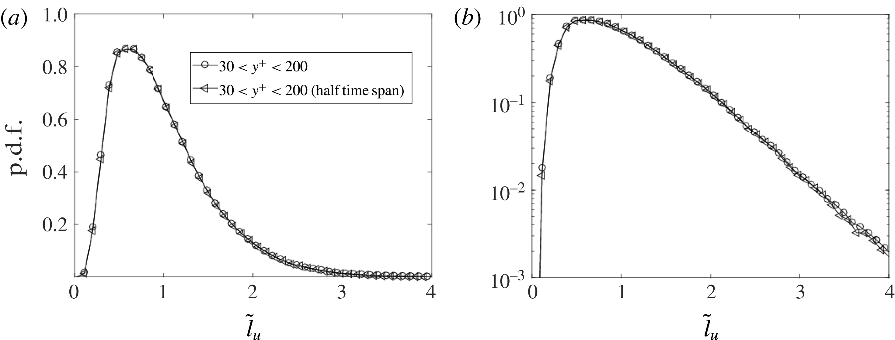
Statistical convergence check for the p.d.f. of
 $\tilde{l}_{u}$
.

Acknowledgements
The funding support of the National Basic Research Programme of China (973 programme; grant 2014CB744802) and the support of the National Natural Science Foundation of China (under the grant nos. 11772194 and 91441116) are acknowledged. W.L. also thanks the Centre for High Performance Computing at Shanghai Jiao Tong University for supporting the large-scale computations.
Appendix. Resolution independence and statistical convergence
The current mesh satisfies the DNS resolution requirement, especially along the wall-normal direction. To justify the sufficiency of the resolution, considering that the vector lines and vorticity lines in the near-wall region are basically parallel to the wall, a new mesh set-up is used with doubled grid points along both the streamwise and spanwise directions. The length p.d.f.s of streamline segments are shown in figure 17, and the length p.d.f.s of vorticity line segments are shown in figure 18. It can be seen that the curves from the different mesh set-up cases are quite close. For the high-resolution results, slight scattering at the p.d.f. tails is attributed to the short sampling time span (
 $30\unicode[STIX]{x1D6FF}_{in}/U_{\infty }$
) for statistical average.
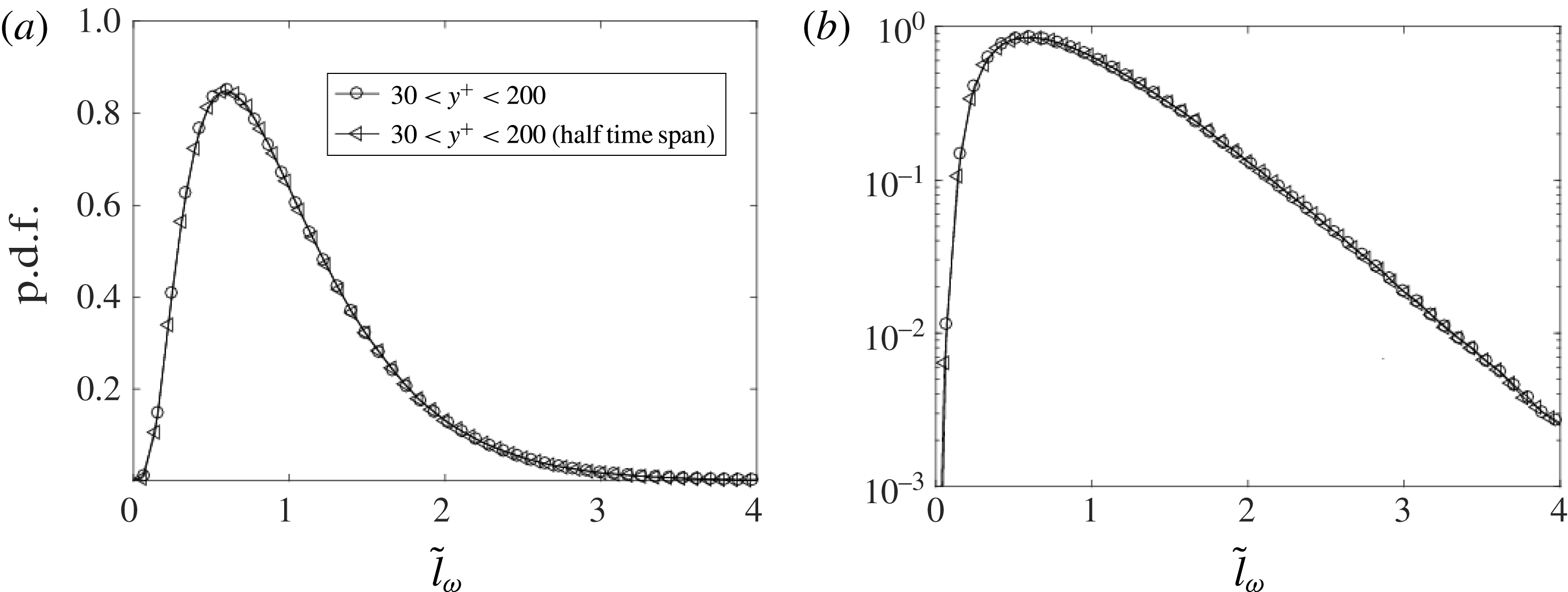
Statistical convergence check for the p.d.f. of
 $\tilde{l}_{\unicode[STIX]{x1D714}}$
.

Meanwhile, to justify the statistical convergence, p.d.f.s of
 $\tilde{l}_{u}$
and
 $\tilde{l}_{\unicode[STIX]{x1D714}}$
from only half time span samples are also calculated, as shown in figures 19 and 20. Clearly, the differences are negligibly small.