1 Introduction
Flows around multiple bluff bodies have received considerable attention, not only because of interference effects leading to complex flow physics, but also because of a wealth of engineering applications. Examples of industrial occurrences of such flows are found around offshore structures and blades of multistage turbo-machines, in heat exchangers, etc. The resulting interference caused by nearby bodies also constitutes interesting examples of nonlinear interaction problems in fluid dynamics. Many and mostly experimental investigations have been carried out, especially on the flow around groups of bluff bodies. The flow interference between two circular cylinders in various cross-flow arrangements, e.g. tandem, side-by-side and staggered configurations, has been reviewed by Zdravkovich (Reference Zdravkovich1977), Sumner (Reference Sumner2010) and recently by Zhou & Alam (Reference Zhou and Alam2016). For side-by-side arrangements, depending on the proximity of the cylinders, both weak and strong interactions between the wakes are reported. The three main flow patterns observed for side-by-side configurations are the single-bluff-body behaviour at small gap ratios
 $g/d$
(the ratio between the distance between the cylinders,
 $g$
, and the cylinder diameter,
 $d$
), biased gap flow at intermediate
 $g/d$
and two in-phase or anti-phase parallel vortex streets at large
 $g/d$
.
1.1 Side-by-side circular cylinders
For two side-by-side circular cylinders at
 $g/d<0.1{-}0.2$
, the two outer shear layers interact with each other and roll up to form a large-scale vortex similar to the wake of a single body with double diameter. For
 $0.1{-}0.2<g/d<1{-}1.2$
, the biased gap flow results in an asymmetric wake configuration comprising one narrow and one wide wake. Strong periodic vortex shedding is detected in the narrow wake while the almost symmetric wake at the wide side is characterized by turbulence-like fluctuations rather than the periodic shedding in the near wake. There is no preferred direction of the deflection of the gap flow: the biased gap flow switches from one side to the other if actively disturbed. A stable biased gap flow has been reported by many researchers, e.g. Williamson (Reference Williamson1985) for
 $Re=50{-}200$
and Sumner et al. (Reference Sumner, Wong, Price and Paidoussis1999) for
 $Re=500{-}1900$
. However, a random switching of the direction of the biased gap flow between side-by-side circular cylinders has been seen in some other studies. This unsteady behaviour, referred to as the flip-flopping phenomenon, was first observed by Bearman & Wadcock (Reference Bearman and Wadcock1973) for
 $0.1<g/d<1$
. Kim & Durbin (Reference Kim and Durbin1988) also found that the wakes flipped randomly between two asymmetric states at
 $g/d<1$
. For
 $g/d>1\sim 1.5$
, however, the two vortex streets resembled the wake behind a single body and exhibited identically the same vortex shedding frequency.
In addition to
 $g/d$
, the effect of
 $Re$
has been studied by Xu, Zhou & So (Reference Xu, Zhou and So2003) for side-by-side cylinders. They investigated the wake structure with
 $g/d=0.2{-}0.6$
over the range
 $Re=150{-}14\,300$
. They found that as
 $Re$
increases for a given
 $g/d$
, the flow structure may change from one single vortex street to two vortex streets, of which one is narrow and the other wide. In two side-by-side circular cylinder configurations with biased gap flow, due to not a priori known separation points on the circular cylinders, any slight change of the separation points and base pressure distribution may trigger the gap flow to either switch direction (for smaller
 $g/d$
) or change from anti-phase to in-phase vortex shedding (for the larger
 $g/d$
). Brun, Tenchine & Hopfinger (Reference Brun, Tenchine and Hopfinger2004) studied the effect of increasing
 $Re$
in the range from 1000 to 14 300 with
 $g/d=0.583$
and suggested that the appearance of shear-layer instabilities triggers the biased gap flow to switch from one side to the other and eventually lead to flip-flopping of the biased gap flow.
1.2 Side-by-side square cylinders
For two side-by-side square cylinders, Alam, Zhou & Wang (Reference Alam, Zhou and Wang2011) studied the flow at
 $Re=4.7\times 10^{4}$
with
 $0.3<g/d<1.2$
(based on the side
 $d$
). They identified four different flow regimes: a single body regime, an asymmetric wake regime, a transition regime and a coupled vortex-street regime for
 $g/d<0.3$
,
 $0.3<g/d<1.2$
,
 $1.2<g/d<2.0$
and
 $g/d>2.0$
, respectively. In the asymmetric regime
 $(0.3<g/d<1.2)$
, the gap flow is biased and forms one narrow and one wide wake behind the two square cylinders, and the gap flow may switch randomly from one side to the other (flip-flopping). For
 $1.2<g/d<2$
, which covers the transition regime, they found that three different modes may occur, with gap flow either biased downward, unbiased or biased upward. For
 $g/d>2$
, the vortex shedding frequencies in the two wakes become identical. Depending on the phase shift between the two vortex streets, in-phase or anti-phase vortex shedding can be observed. Alam & Zhou (Reference Alam and Zhou2013) studied the flow structure and gap flow switching in the wake of two side-by-side square cylinders at
 $Re=300$
and
 $0<g/d<4$
. They observed the same four regimes as classified by Alam et al. (Reference Alam, Zhou and Wang2011) at a significantly higher
 $Re=4.7\times 10^{4}$
with only minor changes in the
 $g/d$
-ranges. Alam & Zhou (Reference Alam and Zhou2013) suggested the physical mechanism behind the biased gap flow to be associated with the conjoining of the counter-rotating gap vortices at sufficiently small
 $g/d$
resulting in a low-pressure region between them. Therefore, the two counter-rotating vortices attract each other and are advected downstream with larger velocity. The phase difference between the two vortices determines the direction of the biased gap flow. They related the switch between the narrow and wide wakes, or between the anti-phase and in-phase vortex streets, to a change in the phase shift between the two gap vortices which start at the separation points or roll-up of the separated shear layers. Alam & Zhou (Reference Alam and Zhou2013) mentioned that the small influence of
 $Re$
on the flow configuration behind side-by-side square cylinders is reasonable in view of the fixed flow separation points. For flow around a single square cylinder, in spite of its sharp corners, the separation point may either be at the leading edges with no subsequent reattachment, or separation and reattachment occur on the side surfaces. Yen & Liu (Reference Yen and Liu2011) measured the pressure distribution over the surfaces of two side-by-side square cylinders at different
 $g/d$
and
 $Re$
. Their results with biased gap flow
 $(g/d=0.5)$
showed that the pressure distributions over the inner surfaces (i.e. gap-facing sides) gradually change along the gap and are different at the two inner surfaces of the square cylinders. One may speculate that even with fixed separation points at the leading edges, any changes in the pressure distribution over the inner surfaces may trigger a biased gap flow to switch to the other side. Symmetrically coupled vortex streets behind side-by-side square cylinders have been studied by Kolar, Lyn & Rodi (Reference Kolar, Lyn and Rodi1997) by ensemble-averaged measurements at
 $Re=23\,100$
and
 $g/d=2$
. The two-cylinder results were compared with results obtained for flow around a single square cylinder in terms of local flow topology, circulation etc.
1.3 Side-by-side flat plates
Hayashi, Sakurai & Ohya (Reference Hayashi, Sakurai and Ohya1986) investigated wake characteristics behind groups of normal flat plates (two, three and four plates) placed side-by-side with different
 $g/d$
at
 $Re=6000{-}19\,000$
by means of hot-wire anemometry. According to their experimental results, a single wake was observed at
 $g/d=0.2$
. At
 $g/d=0.5{-}1.5$
, a stable gap flow was biased upward or downward, whereas a flip-flopping gap flow was reported at
 $g/d=1.75$
. For
 $g/d>2$
, one vortex street formed behind each of the plates, but merged further downstream.
Miau, Wang & Chou (Reference Miau, Wang and Chou1992) also investigated the wake behind two side-by-side flat plates. Their flow visualizations were performed at
 $Re=440$
and presented for
 $g/d=0.5$
and 2. Moreover, they presented velocity signals obtained by hot-wire anemometry for various
 $g/d$
at
 $Re=300{-}12\,000$
. For
 $g/d=0.4{-}1.3$
, the upward- or downward-biased gap flow stayed stable and resulted in a narrow and a wide wake. In their experiments flip-flopping of the gap flow was observed for
 $g/d=1.5{-}1.85$
. For
 $g/d>2$
, they measured identical shedding frequencies in both vortex streets, similarly as in the wake behind a single flat plate.
Miau, Wang & Chou (Reference Miau, Wang and Chou1996) studied the flip-flopping phenomenon in the wake behind two side-by-side flat plates for
 $g/d=1.4{-}2.1$
and
 $Re=6600{-}18\,000$
. They characterized the flow in three different regimes: biased, non-biased and unsteady states (transition between biased and non-biased states). At
 $g/d=1.4{-}1.6$
, the gap flow always appears biased and may switch randomly from one side to the other. At
 $g/d=1.6{-}1.9$
, however, the percentage of the time that the gap flow is non-biased increased and the flow exhibited transitions from a biased to a non-biased state and vice versa. Miau et al. (Reference Miau, Wang and Chou1996) also considered the influence of free-stream turbulence on the number of switches of the gap flow. They found that an increased turbulence intensity promoted the flip-flopping of wakes behind side-by-side plates for
 $g/d=1.4{-}1.7$
.
Higuchi, Lewalle & Crane (Reference Higuchi, Lewalle and Crane1994) investigated the wake behind two flat plates placed side-by-side at
 $Re=1500$
and
 $g/d=1$
and 2 experimentally. For the smaller
 $g/d$
, they observed a symmetric wake early in the test, but the wake eventually became asymmetric with a biased gap flow after several shedding periods. The resulting asymmetric flow pattern comprising one narrow and one wide wake stayed stable all the time. For
 $g/d=2$
, the two near wakes were similar in size, and the vortex shedding in the near wake was mostly anti-phase. However, due to the slight phase difference between the two wakes, the phase relation was time-dependent and intermittent structures could be observed. Further downstream, the two inner shear layers began to interact and a combined wake was formed.
In contrast to the random switching of the gap flow behind two side-by-side circular and square cylinders, flip-flopping has not been observed in the case of side-by-side flat plates with
 $g/d<1.4$
. This is surprising since an asymmetric wake with biased gap flow is seen for quite small
 $g/d\geqslant 0.4$
. However, due to the fixed separation points at the side-by-side plates configuration, the need for stronger perturbations in order to switch the gap flow can be expected. Consistently, the flip-flopping phenomenon in this case is reported only for larger
 $g/d$
for which the biased gap flow configuration is less stable and the unbiased gap flow state is more stable (Miau et al.
Reference Miau, Wang and Chou1992). Hayashi et al. (Reference Hayashi, Sakurai and Ohya1986) suggested the inception of vortex-street formation in the wide wake to be a possible cause of the flip-flopping observed at larger
 $g/d$
for side-by-side flat plates.
1.4 Motivation for the present investigation
In spite of the numerous experimental studies on flow around pairs of cylinders with different cross-sectional shapes, the flow around two side-by-side flat plates has received considerably less attention. The near wake behind a normal flat plate resembles in many ways the near wake of a circular cylinder whilst its separation points are fixed. Unlike in the wake of side-by-side circular cylinders, e.g. Zhou (Reference Zhou2003) and Brun et al. (Reference Brun, Tenchine and Hopfinger2004), the instability that arises in the shear layers that separate from the edges of the side-by-side plates has not yet been explored in detail, although
 $Re$
in the laboratory experiments by Higuchi et al. (Reference Higuchi, Lewalle and Crane1994) and Miau et al. (Reference Miau, Wang and Chou1992) is in the range in which shear-layer instabilities are to be expected. Miau et al. (Reference Miau, Wang and Chou1992) vaguely suggested that the development of turbulent fluctuations in their wide wake evolved from an instability of the shear layers. One objective of the present study is therefore to study the shear-layer instability in the near wake of side-by-side plates and, moreover, to investigate if this instability has any influence on the stability of the biased gap flow. A quantity of immediate concern to address this issue is the characteristic shear-layer frequency.
Since the flow inevitably separates from the edges of a flat plate placed normal to the flow, the wake behind the flat plate is insignificantly affected by
 $Re$
compared to the wake flow behind a circular cylinder in which the location of the separation points vary with
 $Re$
. While the major features of the wake behind a single flat plate exhibit substantial
 $Re$
-variations in the range
 $100<Re<750$
(e.g. Najjar & Vanka Reference Najjar and Vanka1995; Narasimhamurthy & Andersson Reference Narasimhamurthy and Andersson2009), it is anticipated that
 $Re=1000$
is sufficiently high to make the wake flow representative of the
 $Re$
-independent regime above
 $Re=10^{3}$
for a single flat plate wake; see e.g. Hemmati, Wood & Martinuzzi (Reference Hemmati, Wood and Martinuzzi2016). Therefore,
 $Re=1000$
is sufficient for the wake to exhibit complex flow features, including shear-layer instabilities, and representative also of a higher
 $Re$
wake. At the same time, the three-dimensional flow field can be fully resolved on an affordable computational mesh.
For side-by-side plates at
 $Re=200$
, a scatter in the measured frequency was reported by Williamson (Reference Williamson1985) for
 $1<g/d<1.3$
and ascribed to the absence of a predominant shedding mode. At
 $Re=1500$
and
 $g/d=1.0$
, as mentioned before, Higuchi et al. (Reference Higuchi, Lewalle and Crane1994) observed a symmetric wake in the early stage of their experiment, but the wake turned asymmetric after several vortex shedding periods. However, in the higher-
 $Re$
experiment
 $(Re=8000)$
with the same
 $g/d$
, only an asymmetric wake configuration with biased gap flow was observed by Miau et al. (Reference Miau, Wang and Chou1992). Another objective of the present computational study is therefore to explore the wake behind side-by-side plates at
 $g/d=1.0$
with a view to clarifying the qualitatively different wake configurations observed in these laboratory experiments. For comparison, a narrow-gap case with
 $g/d=0.5$
, i.e. with a stronger interference between the two wakes, will also be investigated. In addition, a simulation of the wake behind side-by-side plates with
 $g/d=1.6$
will be undertaken to justify the occurrence of flip-flopping in a computational study.
The computational study relies on direct numerical simulations (DNSs), in which the unsteady Navier–Stokes equations are integrated on a three-dimensional grid sufficiently fine to eliminate the need for any semi-empirical turbulence model. Note that the flat plate problem is particularly difficult to simulate using turbulence models. To our knowledge, there is no satisfactory Reynolds averaged Navier–Stokes (RANS) or unsteady Reynolds averaged Navier–Stokes (URANS) simulation for this flow, although there exist relatively good large-eddy simulations (LESs). A couple of studies of the wake structure behind a single normal flat plate have been carried out by means of DNS, e.g. Najjar & Balachandar (Reference Najjar and Balachandar1998), Narasimhamurthy & Andersson (Reference Narasimhamurthy and Andersson2009) and Hemmati et al. (Reference Hemmati, Wood and Martinuzzi2016). A particularly attractive feature of this computational approach is the access to complete fully resolved three-dimensional flow fields.
The manuscript is organized in this way. Following the Introduction, the side-by-side configuration is introduced in § 2 together with the governing flow equations and their boundary conditions. The DNS solver is described together with our choice of computational domain and the grid. Then in § 3, the dynamics of the simulated wake behind side-by-side plates at different
 $g/d$
is explored. In § 3.1, a symmetric wake configuration with anti-phase vortex streets for
 $g/d=1.0$
is presented, accompanied by a discussion of remarkably different features of the three-dimensional instability in the upper and lower wakes. We next proceed to present results of an asymmetric wake with biased gap flow for
 $g/d=1.0$
and 0.5, in § 3.2. An attempt is made to explore an analogy between the separated shear layer in the wide wake and a plane mixing layer. The shedding frequency obtained from the velocity spectra in the immediate wake is compared with the corresponding most amplified frequency in the plane mixing layer. In § 3.3, a simulation showing a flip-flopping near wake behind side-by-side plates for
 $g/d=1.6$
is briefly discussed. Finally, the main findings of our investigation and their implications are summarized in § 4.
2 Flow configuration and numerical method
The present bluff-body geometry consists of two side-by-side flat plates placed normal to the inflow. The thickness of the plates is considered to be very small. The Reynolds number
 $(Re)$
based on the inflow velocity
 $(U_{0})$
and one plate width
 $(d)$
, is 1000 and
 $g/d=0.5$
and 1.0. The three-dimensional Navier–Stokes equations, solved in time with an incompressible formulation, are given in (2.1) and (2.2). Note that the equations are in Cartesian tensor form and the repeated indices (
 $i$
and
 $j=1$
, 2 and 3) imply summation:
 $$\begin{eqnarray}\displaystyle & \displaystyle \frac{\unicode[STIX]{x2202}u_{j}}{\unicode[STIX]{x2202}x_{j}}=0, & \displaystyle\end{eqnarray}$$
 $$\begin{eqnarray}\displaystyle & \displaystyle \frac{\unicode[STIX]{x2202}u_{i}}{\unicode[STIX]{x2202}t}+u_{j}\frac{\unicode[STIX]{x2202}u_{i}}{\unicode[STIX]{x2202}x_{j}}=-\frac{1}{\unicode[STIX]{x1D70C}}\frac{\unicode[STIX]{x2202}p}{\unicode[STIX]{x2202}x_{i}}+\unicode[STIX]{x1D708}\frac{\unicode[STIX]{x2202}^{2}u_{i}}{\unicode[STIX]{x2202}x_{j}\unicode[STIX]{x2202}x_{j}}. & \displaystyle\end{eqnarray}$$
Direct numerical simulation of the flow past the configuration has been carried out by using the finite-volume code MGLET (Manhart Reference Manhart2004). The code has a second-order central-differencing scheme for spatial discretization and a third-order explicit Runge–Kutta scheme for marching in time. The Poisson equation is solved by an iterative, strongly implicit procedure (SIP). The code uses a staggered Cartesian grid and the body surface is implemented in the grid by means of a direct forcing immersed boundary method (Peller et al.
Reference Peller, Duc, Tremblay and Manhart2006). All of the spatial dimensions are normalized by the plate width
 $d$
, and all velocities are scaled by the inflow velocity
 $U_{0}$
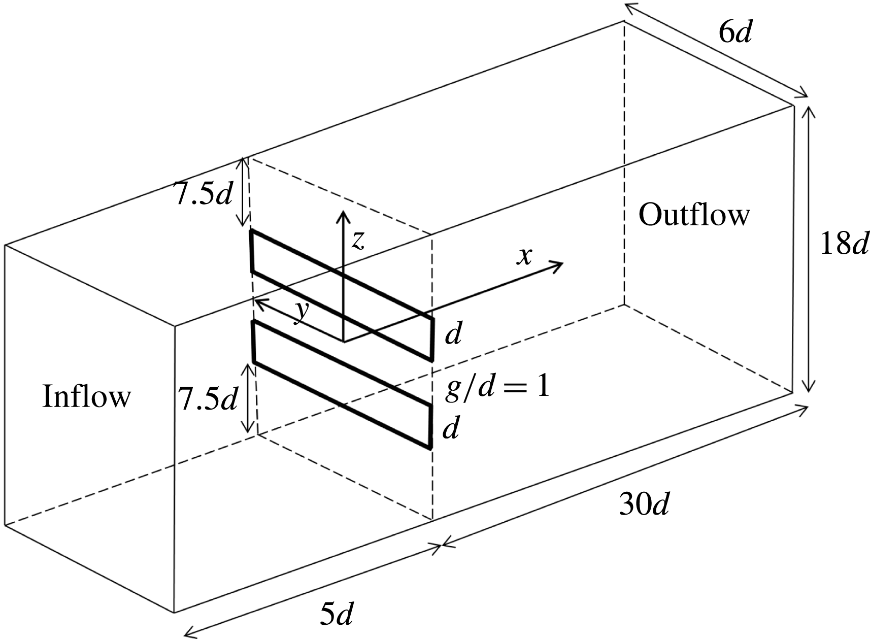
. The computational domain, as shown in figure 1, has a length of
 $35d$
in streamwise,
 $6d$
in spanwise and
 $18d$
in cross-stream directions.
Computational domain (not to scale).

A uniform inflow velocity, free from any perturbation, is imposed at the inlet
 $x/d=-5$
. Periodic boundary conditions are used at the two vertical sides of the computational domain in order to simulate infinitely long plates. Along the top and bottom planes, free-slip boundary conditions are satisfied. A Neumann boundary condition is used for the velocity components at the outlet. It must be mentioned that, due to the geometrical symmetry in all simulations, there is no preference in the direction of the biased gap flow or the appearance of the instability modes in the upper and lower wakes.
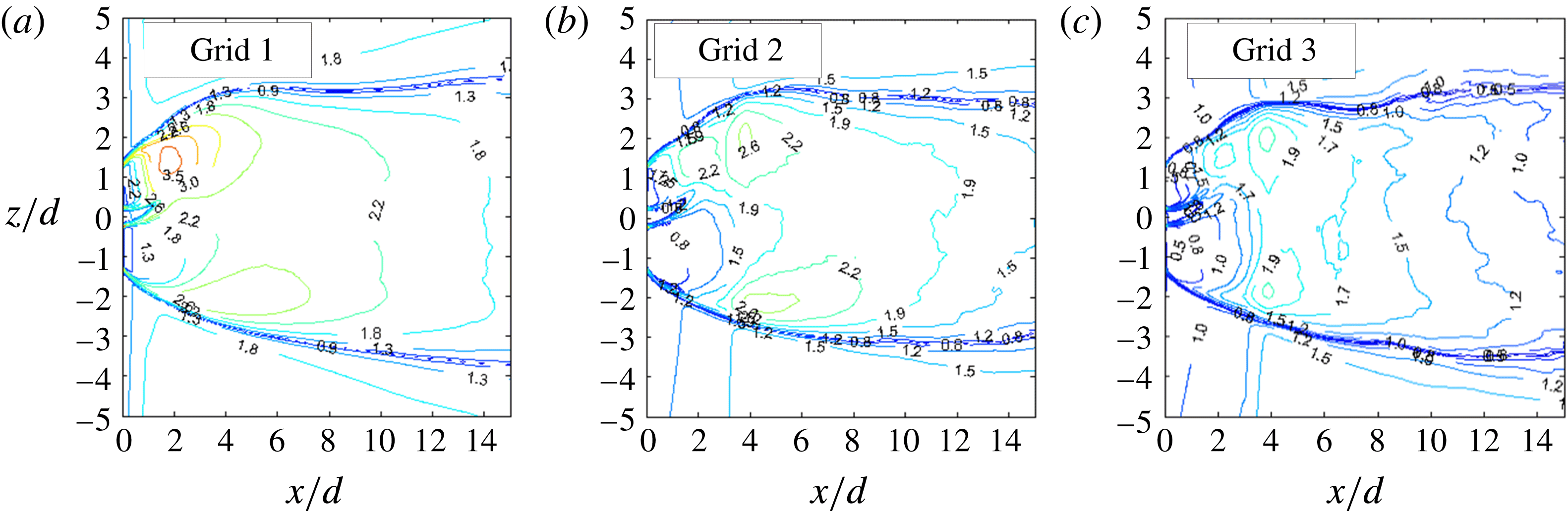
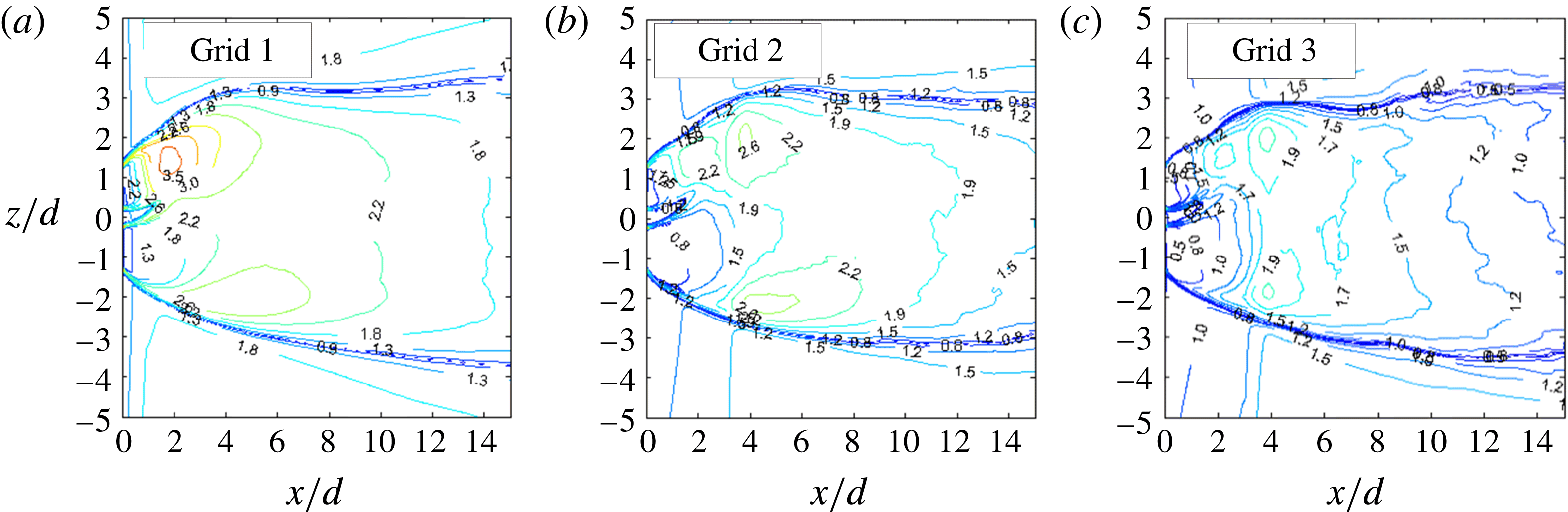
Iso-contours of the local grid resolution
 $\unicode[STIX]{x1D6E5}/\unicode[STIX]{x1D702}$
. The local grid size
 $\unicode[STIX]{x1D6E5}$
is compared with the Kolmogorov length scale
 $\unicode[STIX]{x1D702}$
for
 $g/d=0.5$
from simulations with three different grids, (a) Grid 1, (b) Grid 2 and (c) Grid 3.
Three sets of numerical mesh, Grid 1,
 $704\times 120\times 464$
, Grid 2,
 $768\times 200\times 464$
and Grid 3,
 $768\times 200\times 784$
degrees of freedom, were studied. First the effect of refinement in the streamwise,
 $x$
-direction, and spanwise,
 $y$
-direction, was examined. Then the grid resolution in the cross-stream,
 $z$
-direction, was refined. In order to verify if the simulations capture the essential flow physics by the numerical simulation, the local grid size
 $\unicode[STIX]{x1D6E5}=(\unicode[STIX]{x0394}x\unicode[STIX]{x0394}y\unicode[STIX]{x0394}z)^{1/3}$
can be compared with Kolmogorov’s microscale
 $\unicode[STIX]{x1D702}=(\unicode[STIX]{x1D708}^{3}/\unicode[STIX]{x1D700})^{1/4}$
. Here,
 $\unicode[STIX]{x1D700}$
is the homogeneous dissipation rate of turbulent kinetic energy
 $\unicode[STIX]{x1D700}=\unicode[STIX]{x1D708}\overline{(\unicode[STIX]{x2202}u_{i}/\unicode[STIX]{x2202}x_{j})(\unicode[STIX]{x2202}u_{i}/\unicode[STIX]{x2202}x_{j})}$
, where
 $u_{i}$
is the fluctuating part of the instantaneous velocity component which includes both the unsteady fluctuations and the turbulent fluctuations. Figure 2 shows iso-contours of the ratio of the local grid size
 $\unicode[STIX]{x1D6E5}$
to the Kolmogorov length scale
 $\unicode[STIX]{x1D702}$
for all grids for a part of the domain. As the figure shows, the poorest resolution is approximately 3.5 for Grid 1, 2.6 for Grid 2 and 1.9 for Grid 3. However, the differences between the results from the three grids are very small, e.g. the differences between the shedding frequencies of the narrow and wide wakes from the three simulations were less than 2 %. Note that special care has been taken regarding the characteristics of the shear layer. In the simulation with Grid 3, the number of grid points in the cross-stream,
 $z$
-direction, was double that of the first grid. The computational grid does not influence the topology of the small transition shear-layer vortices and their frequency. We therefore selected Grid 1
 $(704\times 120\times 464)$
to investigate the flow physics. In this grid, the smallest cells, which are placed in the vicinity of the plates, have resolution
 $0.01d$
in the
 $x$
-direction,
 $0.05d$
in the
 $y$
-direction and
 $0.025d$
in the
 $z$
-direction. The grid has uniform spacing in the spanwise direction. The same grid is used for
 $g/d=1.0$
and 1.6 as well. The time step is chosen to be
 $\unicode[STIX]{x0394}t=0.0005d/U_{0}$
in all simulations. This time step is approximately equal to 0.00016 and 0.000135 times the narrow-wake vortex shedding period at
 $g/d=0.5$
and 1, respectively. The total sampling times are
 $500d/U_{0}$
and
 $250d/U_{0}$
for simulations at
 $g/d=0.5$
and 1.0, respectively. The former and the latter correspond to approximately 150 and 60 shedding cycles in the narrow wakes, respectively. For
 $g/d=1.6$
, the simulation has been run for approximately
 $100d/U_{0}$
. However, for
 $g/d=1.6$
, no quantitative data were extracted and only an unstable flow configuration (flip-flopping) is shown at different time instants.
The blockage ratio
 $2d/l_{z}$
in the present study, at 11 %, is believed to somewhat affect the computed flow field. However, since our focus is on detailed flow phenomena in the near wake we intentionally paid more attention to the grid resolution in the vicinity of the plates than to the size of the cross-section of the computational domain in figure 1. The blockage ratio in the experimental configuration of side-by-side circular cylinders by Brun et al. (Reference Brun, Tenchine and Hopfinger2004) is 14 %. In addition, Sumner et al. (Reference Sumner, Wong, Price and Paidoussis1999) collected existing experimental data for side-by-side circular cylinders. They noticed that the blockage ratio varies from 1 to 18 % (their page 311, table 1). In this respect, the present computational configuration with blockage ratio 11.1 % is within the range of other studies. A relatively high blockage ratio may yield an underprediction of the incoming velocity and therefore overprediction of Strouhal number and may stimulate transitions in the shear layers. However, the adverse influence of blockage is intuitively weaker for the present parallel plates configuration between two free-slip boundaries than for parallel cylinders between two no-slip wind tunnel walls for the same blockage ratio. The influence of the blockage on the qualitatively different wake configurations observed herein, as well as on the dominant wake frequencies reported, is modest.
3 Results and discussion
In this section we first present detailed results for side-by-side flat plates at
 $g/d=1.0$
. As mentioned earlier, this
 $g/d$
was chosen in order to see whether the resulting wake has an asymmetric configuration, as observed by Miau et al. (Reference Miau, Wang and Chou1992), or if the wake initially becomes symmetric and later turns into an asymmetric wake configuration as Higuchi et al. (Reference Higuchi, Lewalle and Crane1994) reported. We used the same computational domain as that shown in figure 1, i.e.
 $35d\times 6d\times 18d$
, and the number of grid points is
 $704\times 120\times 464\approx 39\times 10^{6}$
. However, depending on the initial conditions of the simulations, two strikingly different wake configurations were obtained. We first present results and discuss an apparently symmetric wake configuration in § 3.1. This wake flow consists of two anti-phase vortex streets which are symmetric about the geometrical symmetry plane in the near wake, whereas a wide single turbulent wake is formed further downstream. Some early results from this simulation were reported in a conference paper by Dadmarzi et al. (Reference Dadmarzi, Narasimhamurthy, Andersson and Pettersen2011). While the symmetric wake resulted from a simulation initiated by a symmetric flow field, another simulation started from an asymmetric initial field and resulted in a severely skewed wake configuration that will be explored in § 3.2. In addition, in this sub-section results from side-by-side flat plates at
 $g/d=0.5$
will be presented.
3.1 Symmetric wake configuration
 $(g/d=1.0)$

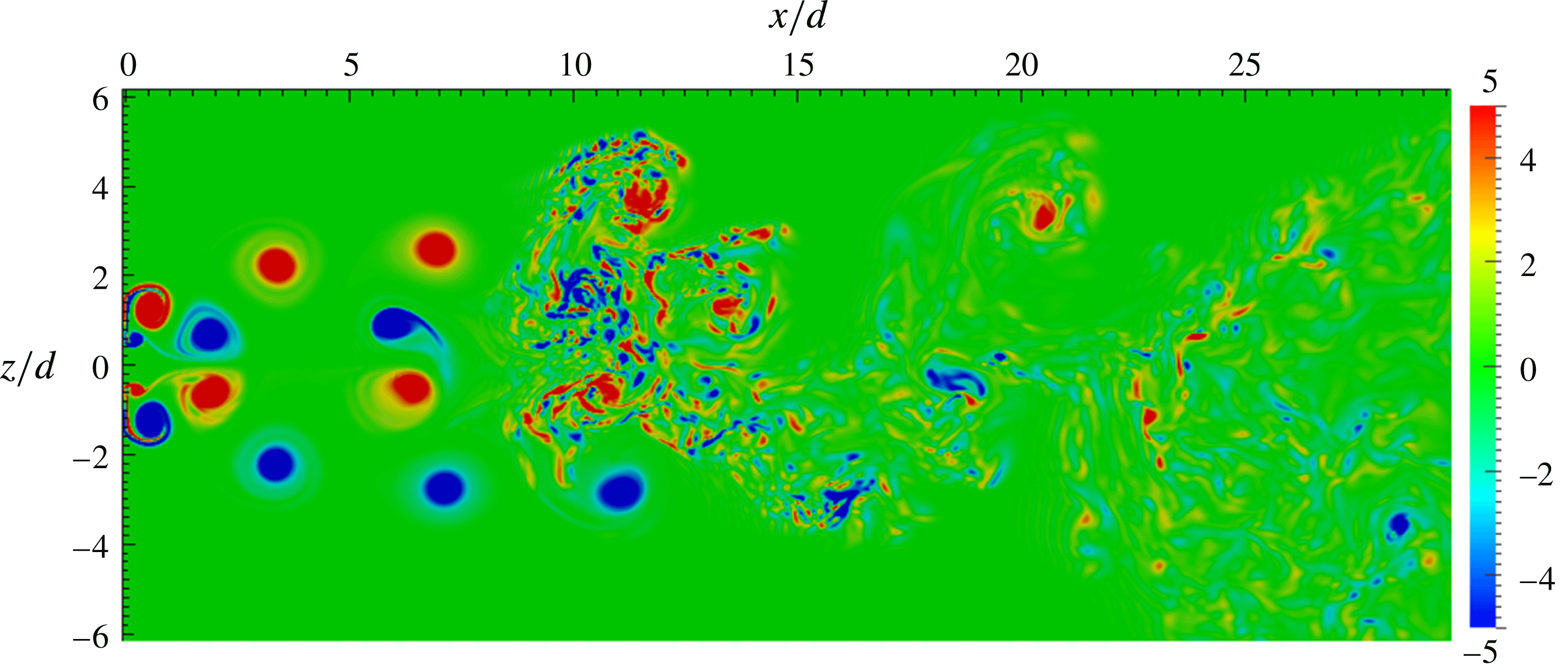
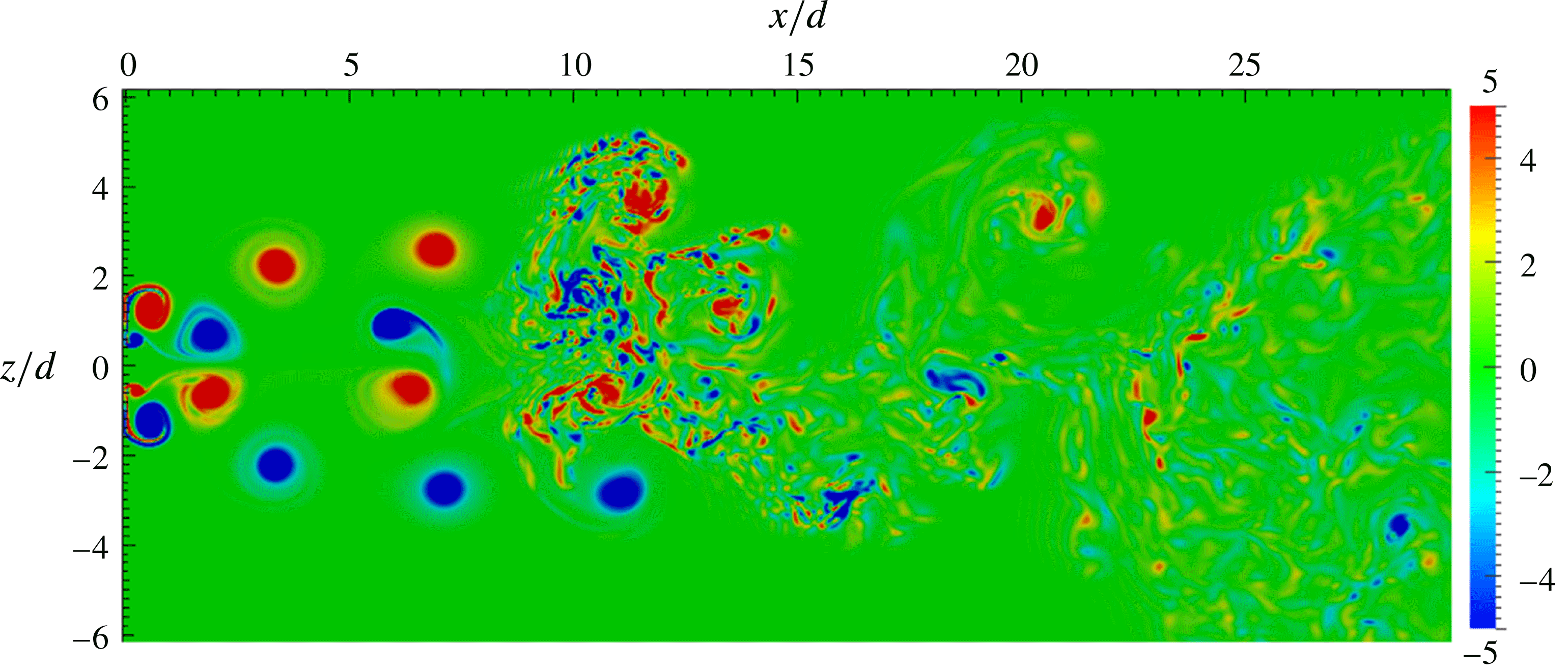
The instantaneous spanwise vorticity
 $(\unicode[STIX]{x1D714}_{y})$
contours shown in figure 3 demonstrate that the two near wakes are equal in size for
 $g/d=1.0$
. Moreover, the two vortex streets are coupled and exhibit symmetry about the mid-plane, i.e. the (
 $x$
,
 $y$
)-plane at
 $z/d=0$
. The gap is not wide enough for the gap vortices to roll up independently and the vortical structures in the inner wake are therefore slightly deformed. The near wake becomes distinctly destabilized
 $5d{-}10d$
downstream of the plates. It is noteworthy that this destabilization first occurs in the central part of the wake, i.e. downstream of the gap. However, the Kármán vortices, which emerged from the outer shear layers, remain almost regular. The qualitative difference between the outer and inner shear layers is probably due to the higher shear rates in the latter. Approximately
 $10d$
downstream of the plates (see figure 3), the wake flow appears to be completely destabilized and fully turbulent. The symmetry of the instantaneous flow about the mid-plane no longer exists and the flow appears as a single vortex street with alternating large-scale vortices. Note that in this study, the immediate wake is referred to as the region up to
 $2d$
downstream while the near wake is considered as the region up to
 $5d$
, the intermediate wake is from
 $5d$
to
 $10d$
and the far wake is beyond
 $10d$
downstream from the plates. Moreover, the terms ‘inner shear layer’ or ‘inner vortices’ refer to those on the side towards the gap flow and consequently the ‘outer shear layer’ or ‘outer vortices’ are those on the free-stream side.
Instantaneous spanwise vorticity
 $\unicode[STIX]{x1D714}_{y}$
at the mid-plane
 $(y/d=0)$
with
 $g/d=1.0$
. A deformation of the inner vortices is observed.
The wake behind a single normal plate at
 $Re=1000$
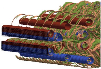
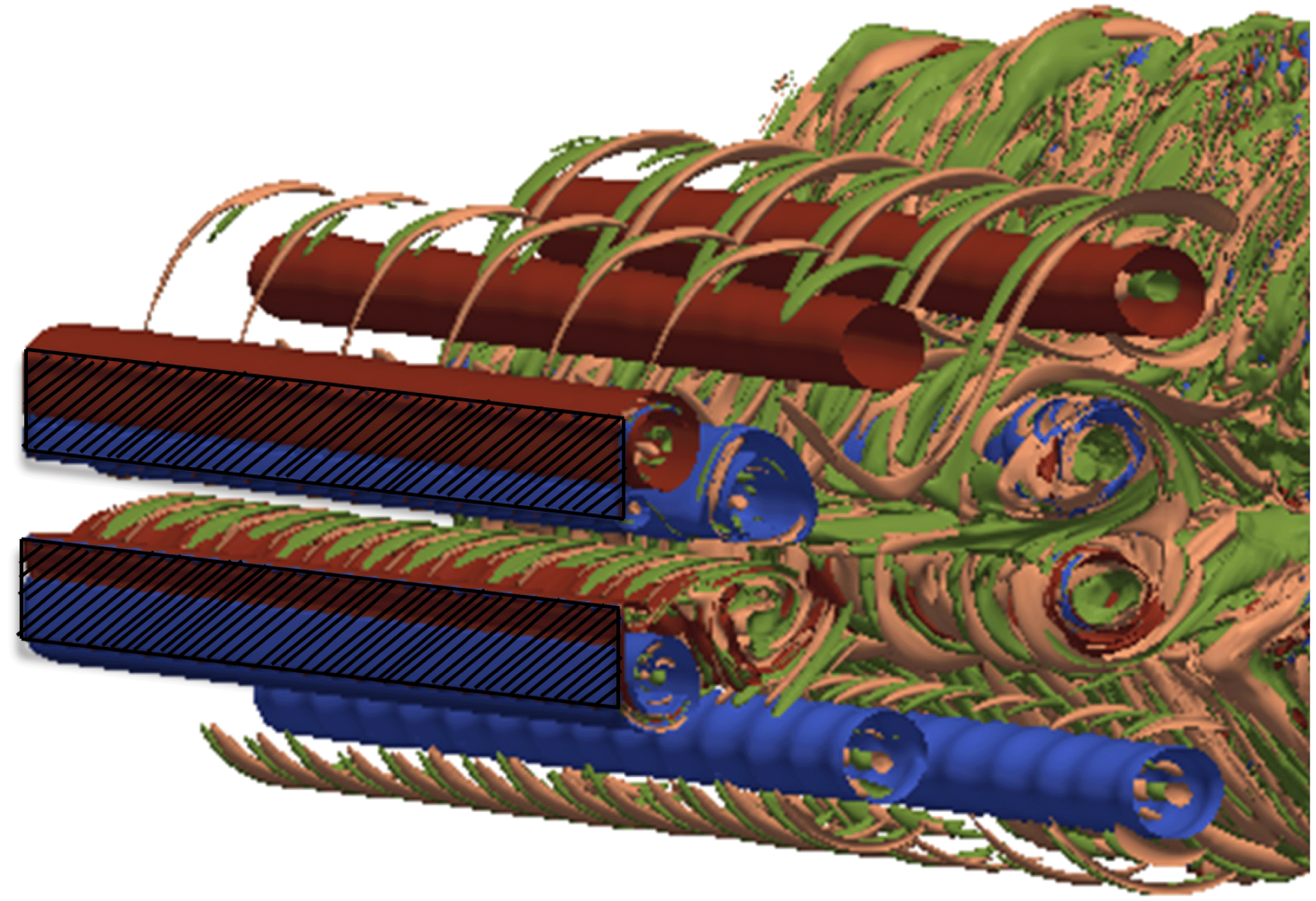
is known to be turbulent: see e.g. Najjar & Vanka (Reference Najjar and Vanka1995), Narasimhamurthy & Andersson (Reference Narasimhamurthy and Andersson2009) and Hemmati et al. (Reference Hemmati, Wood and Martinuzzi2016). In contrast, the vortices in the present near wake exhibit a pretty regular arrangement similar to transitional flow (see figure 3). The perspective view of the instantaneous vorticity field in the near wake in figure 4 shows that the vortex filaments are not uniform along the span of the plates and they exhibit waviness. The two inner vortex cores that make up a pair about the
 $x$
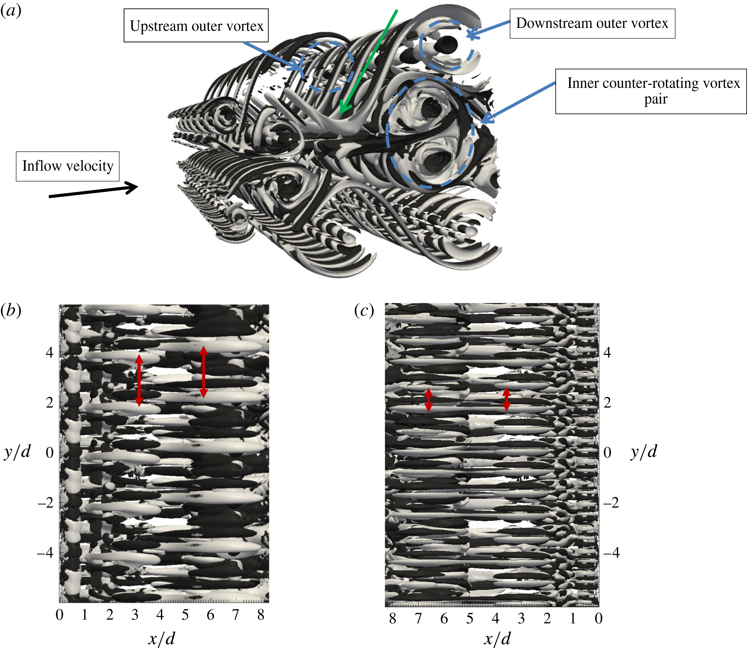
-axis experience a stronger deformation than the two rows of outer vortex cores in the upper and lower wakes. Deformation and reorientation of the spanwise vortex cores in the streamwise direction result in the appearance of streamwise vortex structures in the near wake.
The coexistence of large-scale primary vortex cells
 $\unicode[STIX]{x1D714}_{y}$
and small-scale streamwise-oriented structures
 $\unicode[STIX]{x1D714}_{x}$
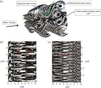
are evident from figure 4. In order to facilitate a closer look at the secondary streamwise vortices, contours of the streamwise component of the vorticity vector are shown in figure 5(a), together with planar views from above and below in figure 5(b,c) covering the near wake from the plates and up to
 $x/d=8$
. The figure depicts pairs of positive and negative streamwise vortices occurring repeatedly along the span of the wake in the braids between the spanwise-oriented primary vortices. The presence of these pairs of counter-rotating streamwise-oriented vortical structures is a signature of the transition to the turbulent flow regime.
Perspective view of the near wake at the same time instant as the side view in figure 3. Instantaneous iso-surfaces of spanwise vorticity
 $\unicode[STIX]{x1D714}_{y}=\pm 2$
(dark red and blue) together with streamwise vorticity
 $\unicode[STIX]{x1D714}_{x}=\pm 0.6$
(green and light brown). Shaded areas show the position of the plates.
Such secondary streamwise vortex structures inevitably promote the mixing. Their role in the development of wake three-dimensionalization has been reported extensively by many researchers, e.g. Williamson (Reference Williamson1996), Robichaux, Balachandar & Vanka (Reference Robichaux, Balachandar and Vanka1999) and Thompson et al. (Reference Thompson, Hourigan, Ryan and Sheard2006). In the wake of a circular cylinder the characteristics of three-dimensional instability modes A and B were studied experimentally and via Floquet stability analysis by Williamson (Reference Williamson1996) and Barkley & Henderson (Reference Barkley and Henderson1996), respectively. The analogy between the natural modes in the cylinder wake and the corresponding modes in the plane wake and free shear layers was mentioned by Williamson (Reference Williamson1996) (please refer to Bernal & Roshko (Reference Bernal and Roshko1986) and Meiburg & Lasheras (Reference Meiburg and Lasheras1988)). Modes A and B become unstable with a spanwise wavelength
 $3d$
–
 $4d$
and
 $1d$
, respectively, where
 $d$
is the cylinder diameter. Both modes present symmetrical characteristics and have the same period as the primary shedding. In mode A, streamwise vortices change sign every half-shedding period (odd reflection–translation symmetry). In mode B, streamwise vortices maintain the same sign (even reflection–translation symmetry).
Iso-surfaces of the streamwise vorticity component
 $(\unicode[STIX]{x1D714}_{x}=\pm 0.4)$
. Perspective view (a), top view (b) and bottom view (c). The positions of the Kármán vortex cores are marked by dashed lines in the perspective view in panel (a).
In addition, a mode C instability has been observed by Zhang et al. (Reference Zhang, Fey, Noack, König and Eckelmann1995) and Yildirim, Rindt & van Steenhoven (Reference Yildirim, Rindt and van Steenhoven2013) in the transition wake behind a circular cylinder with a nearby wire. The placement of the wire in the near wake of the circular cylinder broke the symmetry of the wake and gave rise to an unnatural shedding mode, namely mode C. The same mode was also observed in the wake behind a rotating circular cylinder and staggered circular cylinders by Radi et al. (Reference Radi, Thompson, Rao, Hourigan and Sheridan2013) and Carmo et al. (Reference Carmo, Sherwin, Bearman and Willden2008), respectively. The period of the secondary vortices in mode C transition is twice the shedding period of Kármán vortices and the spanwise wavelength is approximately
 $2d$
.
In the present study of flow past two side-by-side flat plates, the iso-surfaces of the streamwise vorticity component
 $\unicode[STIX]{x1D714}_{x}$
(figure 5
a) show that the spanwise wavelength of the vortical structures is different in the upper and lower near wakes. In the upper wake in figure 5(b), the streamwise vortex pairs are thicker and the spanwise distance between each pair is almost
 $2d$
. However, the lower wake consists of thinner pairs with spanwise wavelength approximately
 $0.9d$
. These observations suggest an analogy between the transition regimes in the upper and lower wakes with the transition regimes observed in the wake of a circular cylinder. Here, however,
 $Re$
is above the transition regime in a single wake. The appearance of the three-dimensional instabilities in the near wake, instead of in the turbulent wake, is a result of the wake interference for
 $g/d=1.0$
.
As shown in figure 5(c), the lower wake braid consists of finer streamwise structures which maintain their streamwise rotational direction over successive passes. In the upper wake (figure 5
b), on the other hand, the secondary streamwise structures change sign accompanied by a spanwise displacement of the secondary structures within one braid relative to the next one. In all the flow visualizations of wired-cylinder wakes by Yildirim et al. (Reference Yildirim, Rindt and van Steenhoven2013), they observed each set of secondary vortices to be out of phase with the preceding set, thereby indicating the period doubling which characterizes mode C. Generally, the strength of the streamwise vortex pairs in the braid regions in figure 5 is small compared with the Kármán vortices and the deformation of the spanwise-oriented vortex cores is negligibly small in the near wake. However, due to the interaction between the two wakes, the streamwise vorticity pairs in the braid stretching from the inner Kármán vortices are intensified. The two inner vortices, with two different spanwise deformation wavelengths (the upper one
 $2d$
and lower one
 $0.9d$
), interact with each other.
The time variation of the cross-stream velocity
 $w/U_{0}$
sampled in the upper and lower wakes (not shown here) shows strong periodic oscillations in the near wake, while the signals in the far wake contain small random fluctuations. The shedding frequency in the near wake and in the intermediate wake corresponded to a Strouhal number of 0.17, whereas the Strouhal number decreased to approximately 0.1 in the turbulent far wake. Moreover, the velocity signal from the upper wake exhibits a mild ‘high-peak low-peak’ W-shaped pattern which has been amplified
 $5d$
downstream. In the wake of a wired cylinder Yildirim et al. (Reference Yildirim, Rindt and van Steenhoven2013) observed high and low peaks in the velocity signal where the period of consecutive high peaks (or low peaks) was twice the shedding period.
In the present plate configuration, the two flat plates are not separated sufficiently from each other to allow Kármán vortices to be generated independently behind each plate. The symmetry of the upper near wake about the mid-plane of the upper plate (i.e.
 $z/d=1$
) and the symmetry of the lower near wake about
 $z/d=-1$
are therefore broken. This raises a crucial question, namely if a direct comparison between the instability mechanisms in either the upper or lower near wake individually with the mechanisms reported for a single symmetric wake, is appropriate or not.
If we consider that the three-dimensional instability structure in the lower wake has the same period as the primary shedding (i.e.
 $T$
-periodic), while the three-dimensionality in the upper wake has the double period (
 $2T$
-periodic), the three-dimensional instability of the combination of the two wakes will be
 $2T$
-periodic. The experiments by Yildirim et al. (Reference Yildirim, Rindt and van Steenhoven2013) showed that the presence of a wire triggered the occurrence of period doubling in the wake. In the present study one may speculate that the presence of one wake has a similar triggering effect on the other.
The enhanced three-dimensionalization and stretching of the inner spanwise vortices lead the wake to become turbulent, thereby promoting randomly oriented fine eddies in the inner part. The outer rows of the spanwise vortex cores persist longer and eventually, further downstream, lose their coherence. The location of onset of turbulence in the inner part of the wake alternates between
 $x/d=5$
and 8 (figure 3). Turbulence does not penetrate further upstream than
 $x/d\sim 5$
and the regular arrangement of vortical structures in the near wake persists throughout the simulation.
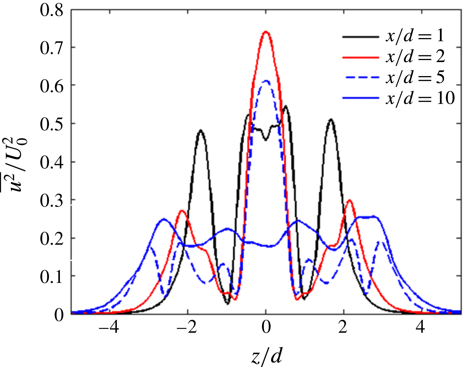
Variance of the streamwise component
 $u$
of the fluctuating velocity at different downstream positions
 $x/d$
.

Figure 6 shows how the streamwise component of velocity fluctuations varies across the wake at different streamwise positions. It should also be noted that statistics are computed after a conventional Reynolds decomposition of the velocity field into mean and fluctuating parts. The second moments of the velocity fluctuations therefore have contributions from both coherent and incoherent fluctuations.
The time-averaged statistics in figure 6 are symmetric about the mid-plane
 $(z/d=0)$
at all four locations considered. The four peaks of the velocity fluctuations at
 $x/d=1$
represent the four shear layers which separate from the two plates at
 $x/d=0$
. At
 $x/d=2$
, the magnitude of the fluctuations has decreased by 50 % in the outer parts of the upper and lower wakes. In contrast, in the inner part of the wake, the fluctuations have increased by approximately 50 % from
 $x/d=1$
and the level of fluctuations in the inner wake is now about four times that in the outer parts of the wake. Closely similar peak levels are observed also
 $3d$
and
 $4d$
downstream (not shown here) and reflect the substantial interactions between the inner vortices and the enhanced instability in the near wake. From
 $x/d=5$
, however, the central peak as well as the outer wake fluctuations are reduced.
 $10d$
downstream, the fluctuation levels in the inner and the outer parts of the wakes have decreased and increased, respectively, as compared with those at
 $x/d=5$
. In the far wake, the fluctuation level remained fairly constant across the whole wake.
In the present study, neither a phase shift between the gap vortices at the separation, nor roll-up of the shear layers, were observed. The
 $1d$
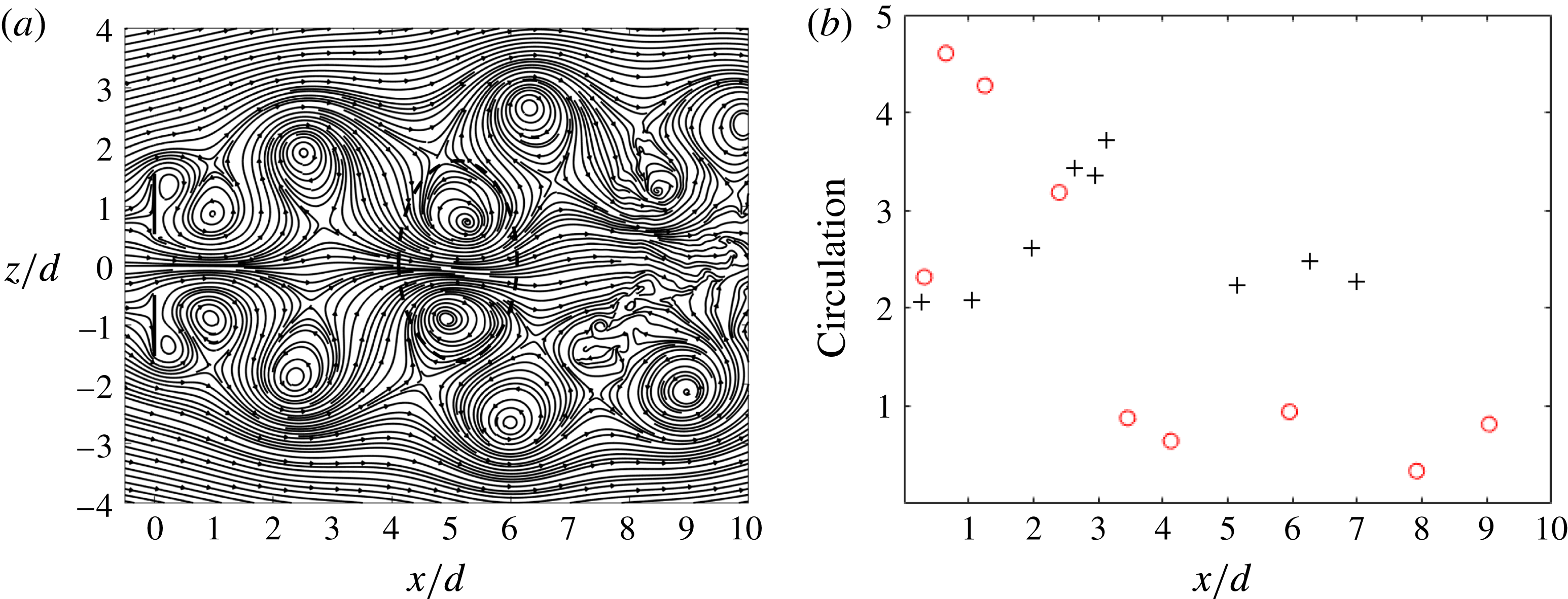
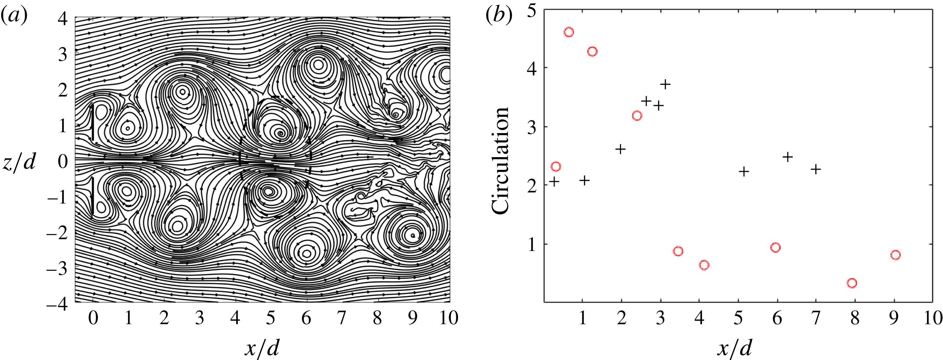
gap width is not small enough to enable immediate interactions and conjoining of the gap vortices. However, as the gap vortices are advected downstream, the two inner counter-rotating vortices behave similarly to a conjoined vortex pair. This results in a low-pressure region and, hence, higher velocities in between the vortices. The larger displacement of the inner counter-rotating vortices compared to their corresponding outer vortices observed in the instantaneous streamline pattern in figure 7(a) where a distinct vortex pair approximately
 $x/d=5$
downstream has been indicated. The existence and stability of coupled vortex streets have been discussed by many researchers, e.g. Landweber (Reference Landweber1942) and Kochin, Kibel & Roze (Reference Kochin, Kibel and Roze1964). Stability conditions were obtained with a model consisting of infinitely long rows of point vortices. To satisfy the stability criteria, the induced transverse velocities should be zero, and all vortices must have the same convection speed. The first condition resulted in only two stable arrangements of the vortices, i.e. in-phase and anti-phase vortex streets. From the second condition, it was concluded that the circulation of the outer vortices must be larger than the inner vortices for the anti-phase vortex streets and vice versa for the in-phase configuration. Figure 7(b) shows the calculated circulation of the outer and inner vortices of one of the Kármán streets in our case. The circulation was calculated from a few available instantaneous velocity fields rather than from the phase-averaged data, and this may cause some uncertainty in the results. In the base region behind the plates
 $(x/d<1)$
the circulations of the outer and inner vortices are very close to each other. Further on in the near wake and up to
 $x/d\sim 3$
, the circulation of the outer vortices is larger than that of the inner vortices. In this region, the circulation of the outer vortices decreases, whereas the circulation of the inner vortices increases. The circulations of the outer and inner vortices become comparable at
 $x/d=2.5{-}3.0$
and subsequently decay in both rows. However, the inner vortices’ circulations remain larger than its corresponding outer counterparts. Overall, from about
 $x/d=3$
, the circulation of the inner rows of vortices becomes larger than that of the outer rows. The larger convection velocity of the inner vortices as they become a pair (figure 7
a) confirmed the above observation made from the circulation plot. Here, however, the two parallel Kármán vortex streets destabilize within
 $5d$
–
 $8d$
downstream, which is consistent with the predicted stability criteria based on potential theory: see Landweber (Reference Landweber1942). The stability of coupled vortex streets with anti-phase vortex shedding behind side-by-side square cylinders has been studied by Kolar et al. (Reference Kolar, Lyn and Rodi1997). They concluded that the theoretical prediction of Landweber (Reference Landweber1942) is applicable beyond the base region of the bluff body. Moreover, in the base region, there is an equal circulation of the vortices which is consistent with the symmetry of the measured mean base-pressure profile by Bearman & Wadcock (Reference Bearman and Wadcock1973).
(a) An instantaneous streamline pattern in the wake behind side-by-side plates
 $(g/d=1.0)$
at the mid-plane
 $(y/d=0)$
. The dashed ellipse indicates the inner counter-rotating vortex pair at
 $x/d=5$
. (b) Streamwise variation of circulation:
 $+$
, inner structure;
 $\circ$
, outer structure.
As already mentioned, in the wake of multiple structures in proximity, the interference of the wakes changes the flow topology and results in different wake configurations. These changes consequently alter the three-dimensional instability characteristics. For example, in the flow around tandem circular cylinders, Carmo, Meneghini & Sherwin (Reference Carmo, Meneghini and Sherwin2010a
,Reference Carmo, Meneghini and Sherwin
b
) showed the possible existence of two different three-dimensional transition modes (region of bistable flow) in the vicinity of drag inversion separation. Choi, Jang & Yang (Reference Choi, Jang and Yang2012) studied the transitional wake behind tandem square cylinders and explained the mode exchange of the three-dimensionality in the vicinity of the critical
 $Re$
by a hysteresis phenomenon. For side-by-side square cylinders, Choi & Yang (Reference Choi and Yang2013) noticed the coexistence of the two instability modes A and B for a specific (anti-phase vortex shedding) base-flow topology at moderate
 $g/d$
and critical
 $Re$
.
In the present study, one might first wonder why two qualitatively different secondary vortical structures appear in the upper and lower wakes even though the two flat plates are placed perpendicular to the inflow and located symmetrically about the (
 $x$
,
 $y$
)-plane at
 $z/d=0$
, as shown in figure 1. The near wake is moreover symmetric, as seen in figures 6 and 7(a). Secondly, one may wonder how these different flow features can coexist next to each other. It seems obvious that the significant gap flow imposes a restriction on the space available for the inner vortices and prevents them from spreading. As a consequence the newly formed inner Kármán vortices are pushed back behind their respective plates. Therefore, the vortex cores in the near wake behind each plate are in closer proximity to each other than in a single wake. The presence of the other wake, and possible induced velocity effects, make it difficult to describe the physical mechanisms of the wake transition. In general, one might say that the nonlinear interactions between the two wakes, which are strongest between the inner vortices, may result in different three-dimensionalizations in the upper and lower wakes. Stability analysis can shed light on the stability characteristics of the side-by-side plates at this specific
 $g/d$
and
 $Re$
. A possible scenario to justify the coexistence of two different transition regimes can be based on the Biot–Savart induced velocity. One may assume that two counter-rotating inner vortices are spatially close to each other and their overall influence, by the induced velocity on the new forming vortex cores and braids, can be rather small. The approximate cancellation of the effects of the inner vortices on the outer vortices suggests the possibility of a partial disconnection between the outer rows of Kármán vortices and the inner row. The possibility of having a complex wake consisting of one row of inner counter-rotating vortex pairs and two outer rows of vortical structures cannot be ruled out. However, a complete analogy between the outer rows of vortices with those observed in a free shear layer, regarding the formation mechanism of the three-dimensional vortex structures, cannot be justified since the Kármán vortices arise from an absolute instability rather than from a convective instability in the free shear layer.
In the upper wake, the feedback mechanism between Kármán vortices (or the physical mechanism of the mode C appearance) discussed by Yildirim et al. (Reference Yildirim, Rindt and van Steenhoven2013) may be relevant. As shown by the streamwise vorticity contours in figure 5, the stretched streamwise vorticity pairs (marked by a green arrow in panel a) which originated from the deformation of the downstream outer vortex, passed the inner vortex (which is the upper vortex of the inner vortex pair) and then reached the upstream outer vortex. This may initiate waviness and vortex loops on the upstream outer vortex. The unusually long vorticity braid (marked by a green arrow) might be caused by the symmetry breaking with respect to each wake centreline and possibly also due to the cancellation effect of the inner counter-rotating vortex pair on the outer vortices. The downstream outer vortex affects the inner vortex by an induced velocity and makes it wavy. However, this inner vortex is close to the other inner vortex from the lower wake and their interactions become stronger as they advect downstream.
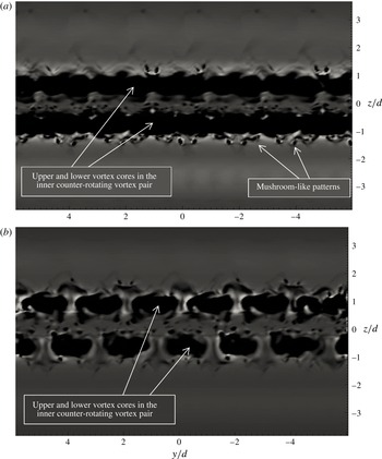
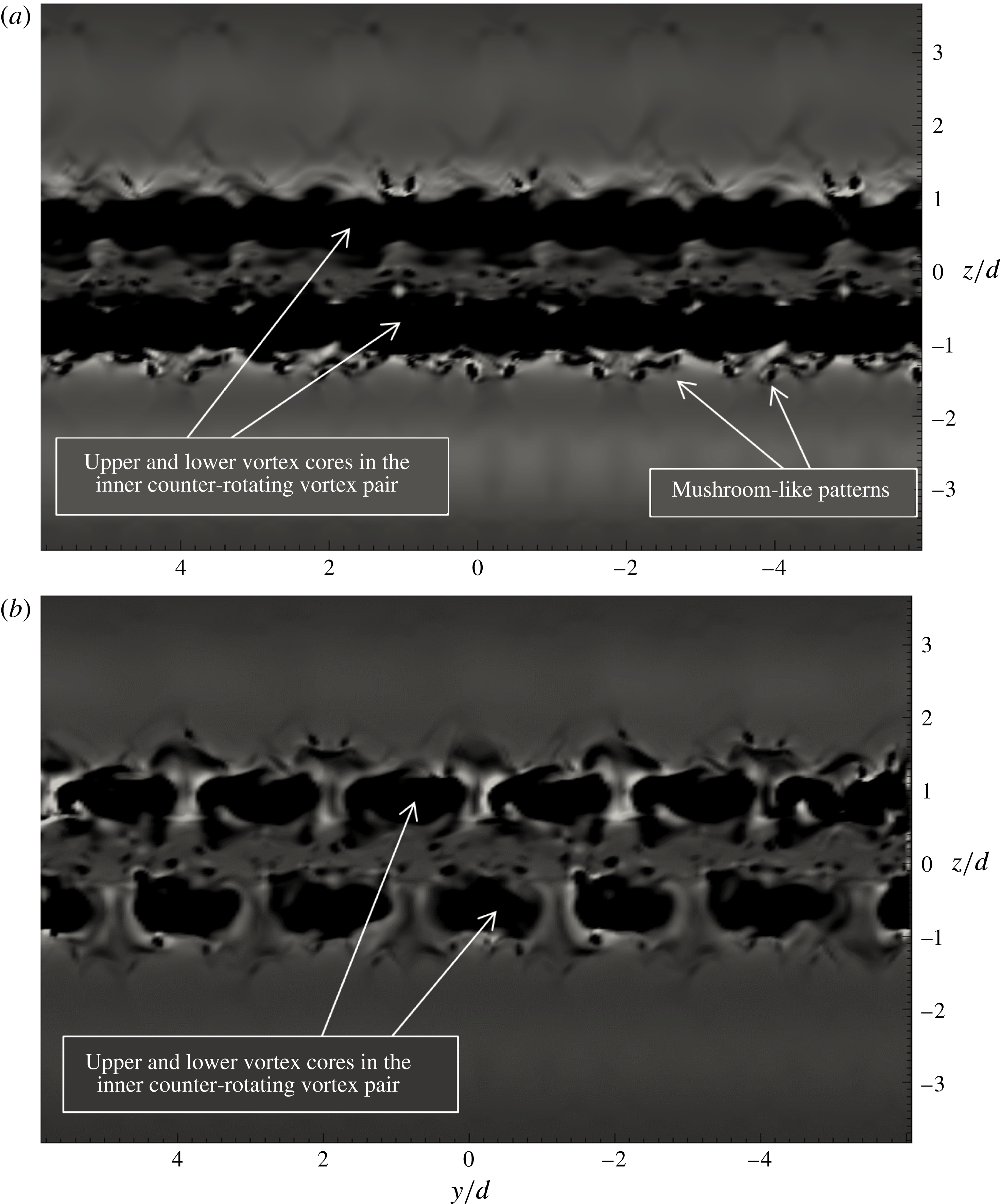
On the other hand, the finer streamwise structures with smaller spanwise spacing in the lower wake are analogous to the instability in the wake of a circular cylinder (Williamson Reference Williamson1996) and a free shear layer (Bernal & Roshko Reference Bernal and Roshko1986). The mushroom-like features of the braids, as well as the vortex cores, are signatures of this mode of instability. Cross-sectional plane views of two inner vortex cores (inner counter-rotating vortex pair) are shown in figure 8 at two different time instants. The dark areas correspond to neighbouring primary vortex cores. Differences in the vortex deformation in the upper and lower inner vortex cores are observed where mushroom-like patterns are indicated. The originally continuous spanwise vortex cores have split into smaller segments further downstream in figure 8(b) and the three-dimensionality is enhanced.
In order to check whether the surprising finding of distinctly different three-dimensionalizations of the upper and lower wake was affected by the spanwise width of the computational domain, this simulation was repeated using a computational domain twice as wide as the original domain, i.e. with a domain size
 $35d\times 12d\times 18d$
. In order to maintain the same grid resolution as before, the number of grid points in the spanwise direction was increased from 120 to 240. The same striking differences between the three-dimensionalizations of the upper and lower wake resulted also from the wider-domain simulation. It must be recalled that, due to the geometrical symmetry of all simulations, there is no preference of the appearance of the instability modes with respect to the upper and lower wakes.
Cross-sectional plane view of vortical structures visualized by means of
 $\unicode[STIX]{x1D706}_{2}$
contours. The planes are chosen through two inner vortices of the primary spanwise vortex cores. In (a) the pair of inner vortices are in an upstream position compared to (b). Note that the plots are at two different time instants.
3.2 Asymmetric wake configuration with biased gap flow (
$g/d=1.0$
and 0.5)

In view of earlier experimental observations, one may wonder if the symmetric wake configuration reported in the preceding § 3.1 is the only stable wake configuration for
 $g/d=1.0$
. To explore the possible existence of other stable configurations, we actively disturbed the flow by introducing positive and negative velocities behind the upper and lower plates, respectively. This asymmetric disturbance may have a similar effect to that of blowing applied behind one plate and suction behind the other plate in a laboratory experiment. This simulation with added velocity disturbances ran for about 10 shedding cycles and resulted in an asymmetric flow field that was used as the initial condition for a new simulation. This new simulation was run without any active disturbances. The geometrical configuration and all the boundary conditions were perfectly symmetric, just as for the simulation reported in § 3.1. The only distinction was that the numerical solution was advanced forward in time, starting from an asymmetric initial flow field. The resulting wake configuration, after the described modification, is surprisingly different from the corresponding symmetric configuration. Stability analysis can provide the theoretical framework to classify the instability property of the modified wake. Huerre & Monkewitz (Reference Huerre and Monkewitz1990) reviewed the instability in spatially developing flows and the connection between local absolute instability and global self-excitation in the flows. In the review paper, they provided different examples of flows with additional parameters (such as base bleed (Wood Reference Wood1964)) and discussed the effect of the control parameter and the global instability. We can speculate that the asymmetric initial condition in our case affects the interaction between the shear layers, which is responsible for the absolute instability in the first place and leads to a significant change of stability properties. For side-by-side circular cylinders Akinaga & Mizushima (Reference Akinaga and Mizushima2005) studied the linear stability analysis for low
 $Re$
. They found that there are two kinds of unstable modes, i.e. antisymmetric and symmetric modes, which lead to in-phase and anti-phase oscillatory flows, respectively, for different
 $g/d$
and
 $Re$
. Mizushima & Hatsuda (Reference Mizushima and Hatsuda2014) investigated the wakes behind side-by-side square cylinders at low
 $Re$
, by linear and weakly nonlinear stability analysis and numerical simulations. They examined the nonlinear interactions of the two modes of disturbance when both modes grow. They found a range of
 $g/d$
and
 $Re$
where the mixed-mode solution is stable and the resultant flow has an asymmetric flow pattern comprising the two modes of disturbance; whereas in the case where both the single-mode solutions are stable, either of the symmetric and antisymmetric mode solutions survives, depending on the initial condition. In the present study of side-by-side plates,
 $g/d$
and
 $Re$
might be in the range where both modes are stable; however, stability analysis can clarify it. Note that in this sub-section, results from a simulation with
 $g/d=0.5$
will also be presented. Since the asymmetric flow configuration with biased gap flow in both cases (
 $g/d=0.5$
and 1.0) is qualitatively the same, the presented results are chosen arbitrarily from both cases.
3.2.1 Wake dynamics
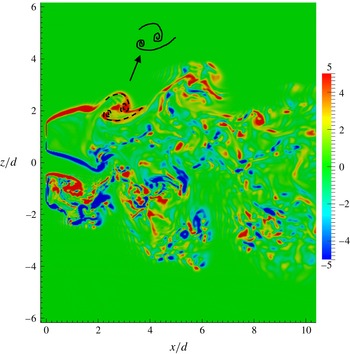
Figure 9 shows the resulting asymmetric wake configuration for
 $g/d=1.0$
, in the absence of external forcing. The spanwise vorticity (
 $\unicode[STIX]{x1D714}_{y}$
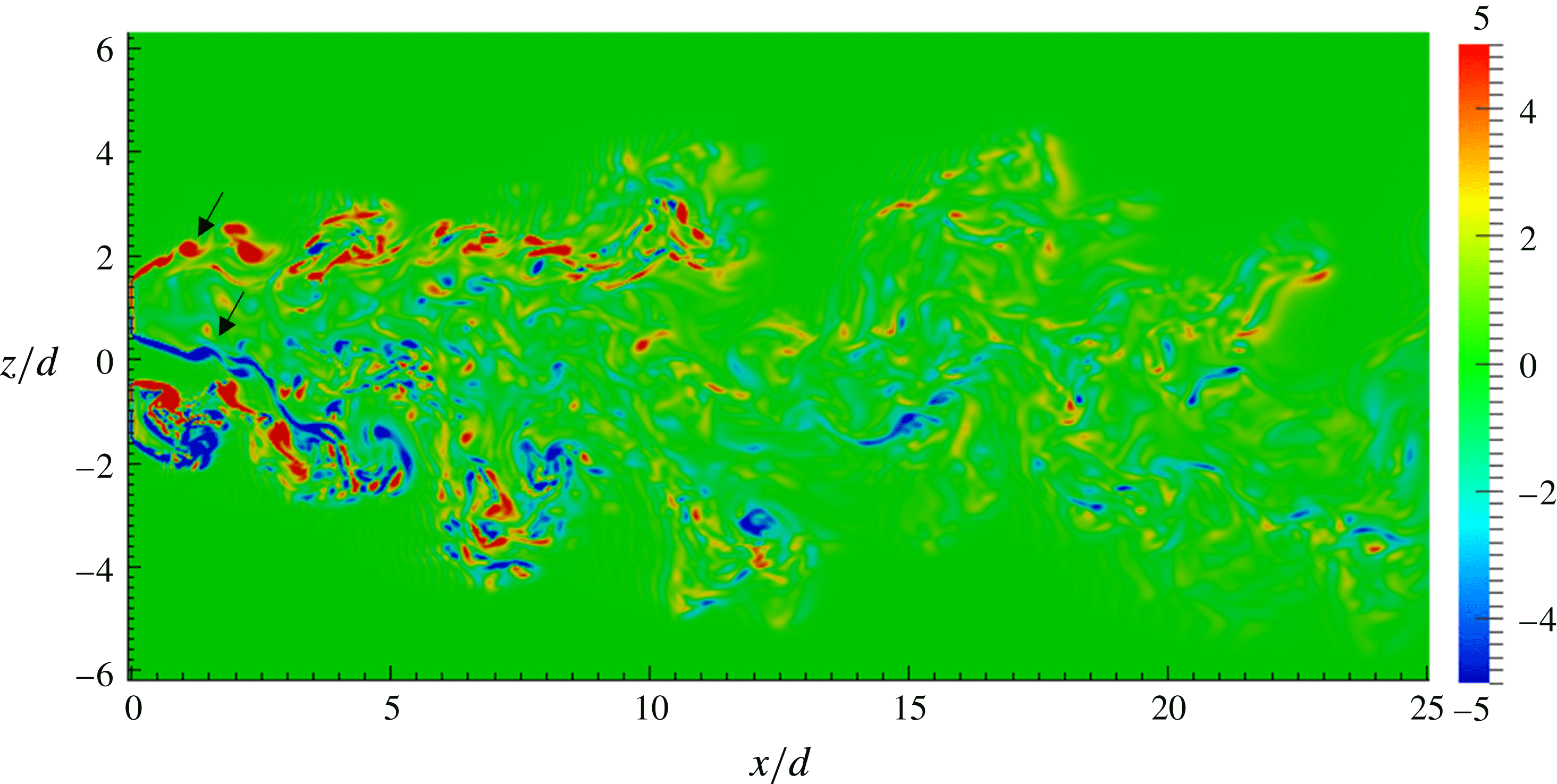
-contours) in figure 9 shows that the gap flow is biased downwards and the near wake consists of a wide and a narrow wake behind the upper and lower plate, respectively. The biased gap flow direction remained the same during the whole simulation.
Instantaneous spanwise vorticity
 $\unicode[STIX]{x1D714}_{y}$
at the mid-plane
 $(y/d=0)$
at
 $tU_{0}/d=250$
. The arrows indicate shear-layer transition vortices.

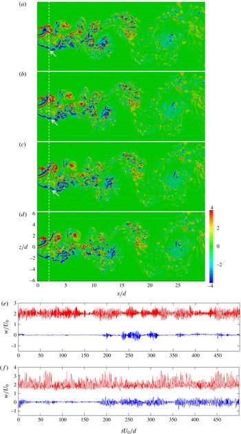
Snapshot sequence of spanwise vorticity contours at the mid-plane
 $(y/d=0)$
at
 $tU_{0}/d=450$
(a),
 $450+T_{NW}/4$
(b),
 $450+T_{NW}/2$
(c) and
 $450+3T_{NW}/4$
(d). Arrows indicate one shear-layer transition vortex at successive snapshots. Time evolution of cross-stream velocity
 $(w/U_{0})$
at the outer shear layer of the narrow wake (red) and the wide wake (blue) at
 $y/d=0$
,
 $(x/d,z/d)=1$
,
 $\pm 1.75$
(e) and
 $(x/d,z/d)=2$
,
 $\pm 1.95$
(f). Note that the red signals are offset by a constant factor 2 for clarity.

The flow behind side-by-side flat plates with
 $g/d=0.5$
is presented with its asymmetric wake configuration in figure 10. Here, a snapshot sequence of spanwise vorticity contours in the mid-plane
 $(y/d=0)$
is shown. The time difference between each successive snapshot is approximately one-fourth of the narrow wake shedding period
 $(T_{NW}/4)$
. Here, however, the wide and narrow wakes are behind the lower and upper plates, respectively, i.e. opposite to the resulting wake configuration obtained for
 $g/d=1.0$
. Since there is stronger interference between the wakes at
 $g/d=0.5$
, some results from this case have been chosen in order to explore the wake dynamics in the asymmetric configuration.
As the snapshot sequence of the vorticity in figures 9 and 10(a–d) shows, the two shear layers in the wide wake do not interact with each other in the immediate wake and exhibit almost a symmetrical shedding. However, there exists a strong alternating vortex shedding in the narrow wake. In the near wake, the inner vortices from the wide wake combine with the subsequent vortices from the narrow wake. Further downstream in the far wake, a large single wake is formed from the outer vortices of the wide wake (lower side of the wake) and amalgamation of the narrow wake vortices. The large combined wake persists until the end of the domain.
As figures 9 and 10(a–d) show, there exist small-scale vortices in the separated shear layer, especially in the outer shear layer of the wide wake. These small transition vortices are the result of Kelvin–Helmholtz (K–H) instabilities and are known to further promote turbulence in the separated shear layer. Examination of the snapshot sequence in figure 10(a–d) reveals that while the narrow wake vortices are shed half a wavelength downstream, the small transition shear-layer vortices are convected almost one wavelength (the position of the shear-layer vortices can be referred to the dotted vertical line). This indicates that the frequency of the shear-layer vortices is about double that of the narrow wake shedding frequency. Similar transition vortices in the separated shear layer of the wide wake have been observed for two and three side-by-side circular cylinders by Brun et al. (Reference Brun, Tenchine and Hopfinger2004) and Zhou (Reference Zhou2003), respectively. The small-scale vortices, which form within the separated shear layer, are similar to those found in a plane mixing layer between two streams with different velocities. The instability of the shear layers in flow past a circular cylinder has been investigated first by Bloor (Reference Bloor1964) and later on by Wei & Smith (Reference Wei and Smith1986) and Prasad & Williamson (Reference Prasad and Williamson1997), among others.
In order to show the temporal characteristics of the separated shear layers in the side-by-side plate configuration, velocity signals are sampled within the outer shear layers, in the narrow and wide wakes. Figure 10(e,f) shows the time traces of the cross-stream velocity
 $(w/U_{0})$
for
 $g/d=0.5$
, within the outer shear layers at
 $x/d=1$
and 2, at the same spanwise position as the corresponding instantaneous vorticity contours shown in (a–d). The red and blue signals correspond to the outer shear layer of the narrow and wide wakes, respectively. The two signals are distinctly different; the blue signal can be called ‘intermittent’ in contrast to the red signal. The presence of high-frequency fluctuation ‘spots’ in the velocity signal in the separated shear layer of the wide wake is associated with the shear-layer (K–H) instability. The snapshot sequence in figure 10 is at time instants with high-frequency events in the wide wake velocity signals. However, the time signal in the shear layer of the narrow wake (red signal) represents a strong periodic vortex shedding. Miau et al. (Reference Miau, Wang and Chou1992) (based on their velocity signal analysis) suggest that on the wide wake side, turbulent velocity fluctuations develop in the near-wake region and no clear indication of periodic vortex shedding was found at the measured location. They suggested that the development of turbulent fluctuations in the wide wake has evolved from the instability of the shear layer, as indicated by Bloor (Reference Bloor1964). However, they did not measure the frequency of the shear-layer transition vortices. A further discussion on the shear-layer frequency will be given later in § 3.2. It must be noted that similar velocity time traces are observed for
 $g/d=1.0$
; however, they are not presented here due to space limitation.
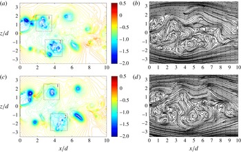
Figure 11 shows instantaneous pressure contours (a,c) and streamlines (b,d) behind the two plates. The instantaneous plots are at two different time instants which correspond to those in figure 10(b,d). The unsteady motion and interactions between the turbulent vortices are revealed by the pressure fluctuations, for which areas with pressure minima correspond to the centres of coherent vortices. The square region 1 shows a location where inner vortices from both plates are squeezed and amalgamated. In figure 11(a), this low-pressure region consists of smaller areas with multiple local pressure minima which correspond to the centres of some different vortices. Somewhat later, in figure 11(c), only one large vortex can be observed. In square region 2 in figure 11(a,c), however, interactions between growing shear-layer vortices and an outer vortex in the wide wake can be seen. Both the pressure contours and the streamlines show that the large outer vortices in the wide wake (lower side of the wake) involve smaller shear-layer vortices. Further downstream, vortices in the narrow wake (upper side of the wake) are pairing. In the far wake a large-scale Kármán street is formed from outer vortices.
Instantaneous pressure
 $(p/\unicode[STIX]{x1D70C}U_{0}^{2})$
contours (a,c) and streamline patterns (b,d) at the mid-plane
 $(y/d=0)$
at the same time instants as figure 10(b,d). Plates are shown by thick lines at
 $x/d=0$
.

The important role of the base pressure in the process of large-scale Kármán vortex formation in bluff-body wakes has been described by many researchers (Gerrard Reference Gerrard1966; Unal & Rockwell Reference Unal and Rockwell1988a
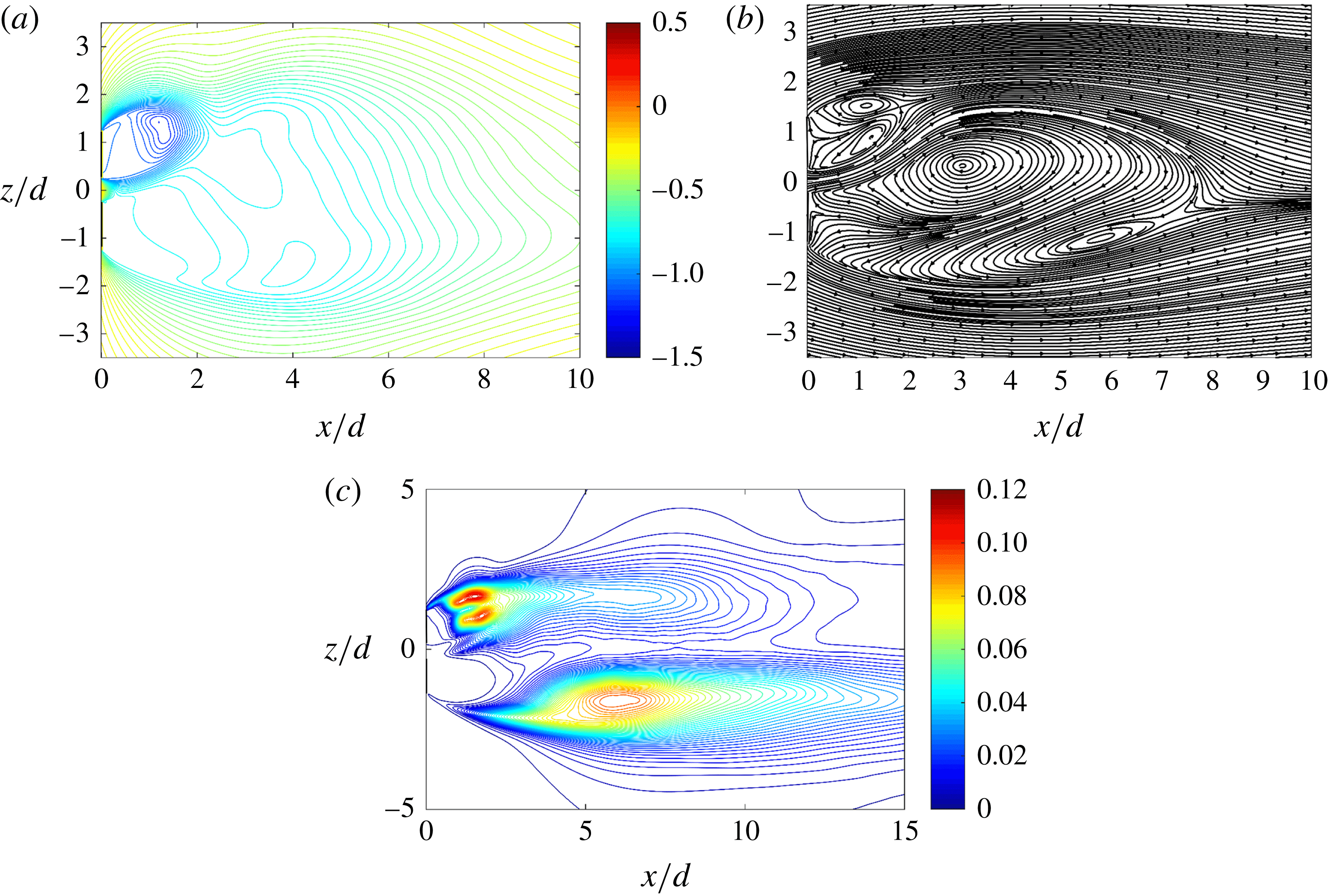
). Wakes behind bluff bodies, in contrast to mixing layers, are characterized by a region of negative base pressure between the separating shear layers. Figure 12 shows contours of mean pressure (a), mean streamlines (b) and root-mean-square (r.m.s.) pressure fluctuations (c). The mean pressure contours show that the region of negative base pressure in the wide wake is less pronounced than in the narrow wake. As expected, the magnitude of the negative base pressure is related to the strength of the vortices formed by the body and their recirculation length. Figure 12(a) shows that the magnitude of the base pressure behind the narrow wake plate is approximately two times larger than the magnitude of the base pressure behind the wide wake plate. The mean pressure coefficient
 $\bar{C}_{P}=2(P-P_{\infty })/(\unicode[STIX]{x1D70C}U_{0}^{2})$
was
 $-1.4$
behind the lower plate (wide wake) and
 $-2.1$
behind the upper plate (narrow wake). In the wide wake, the mean pressure contours exhibit two local pressure minima approximately
 $4d$
downstream of the plate. According to figure 12(c), the pressure fluctuations peak in the recirculation regions. In the narrow wake, two distinct pressure fluctuation peaks
 $(p_{rms}\cong 0.1)$
appear at the location where vortices separated from the shear layers. The recirculation bubble in the narrow wake ends around
 $x/d=2$
, as shown by the mean streamline pattern in figure 12(b). However, the region with relatively high-pressure fluctuations
 $(p_{rms}\cong 0.05)$
extends up to approximately
 $x/d=8$
. This is associated with the amalgamation of the inner vortices of the wide wake with the narrow wake vortices. In the outer separated shear layer of the wide wake, the high-pressure fluctuations are first related to the small-scale shear-layer vortices (
 $p_{rms}\cong 0.03$
up to
 $x/d\sim 2$
). Then the peak of the pressure fluctuation is due to the formation of the large-scale vortices and their interaction with the small-scale shear-layer vortices (
 $p_{rms}\cong 0.08$
at
 $x/d=4{-}8$
). According to the streamline pattern in figure 12(b), the recirculation bubble in the combined wake extends up to
 $x/d=8$
.
Mean pressure
 $(P/\unicode[STIX]{x1D70C}U_{0}^{2})$
contours (a) and mean streamline patterns (b) showing the mean recirculation bubble. (c) Contours of r.m.s. pressure fluctuation. Plates are shown by thick lines at
 $x/d=0$
.

3.2.2 Shear-layer instability
In this sub-section, we will examine the shear-layer instability in the wide wake by comparing with a plane mixing layer. The appearance of small-scale transition vortices in the separated shear layer of a bluff-body wake is visually similar to those in a plane mixing layer of two parallel streams. However, due to the spatial restriction imposed by the formation of the large-scale Kármán vortices in the bluff-body wake, there are also some differences between them. In addition, one might expect an upstream influence from the downstream vorticity dynamics and also from the region of absolute instability (comprising both upstream and downstream waves) in the wake flow (Unal & Rockwell Reference Unal and Rockwell1988a ). In the present study of the wake behind the two plates, transition vortices appear in the separated shear layer of the wide wake. The two shear layers do not interact with each other in the immediate wake and the large-scale Kármán vortex formation region extends downstream. Therefore, a more pronounced similarity between the instability of the separated shear layer in the wide wake and that in a plane mixing layer is expected.
The relation between the shear-layer frequency and the Kármán frequency for a single circular cylinder wake in the form
 $f_{sl}=f_{K}(Re/262)^{0.67}$
was suggested by Prasad & Williamson (Reference Prasad and Williamson1997). However, in the present study, with a narrow and wide wake, the base pressure as well as the shear layer are different from that in a single wake. In addition, there exist two shedding frequencies: one which corresponds to the Kármán vortices formed in the immediate wake of the narrow wake, and the other and lower frequency corresponding to vortices in the combined wake which are noticeable further downstream. Therefore, we aim to examine similarities between the separated shear layers in the wide wake and a plane mixing layer. According to the review paper on perturbed free shear layers by Ho & Huerre (Reference Ho and Huerre1984), the very early stages of the development of a mixing layer is dominated by a linear instability mechanism. In the present sub-section, we first examine if linear stability theory is applicable in the near wake of the wide wake. Then, we proceed to choose a characteristic length for the shear-layer instability. At the end, we compare the shear-layer frequency obtained from the energy spectra in the wide wake with the frequency of the most amplified wave in the plane mixing layer. The latter is based on a linear stability approximation.
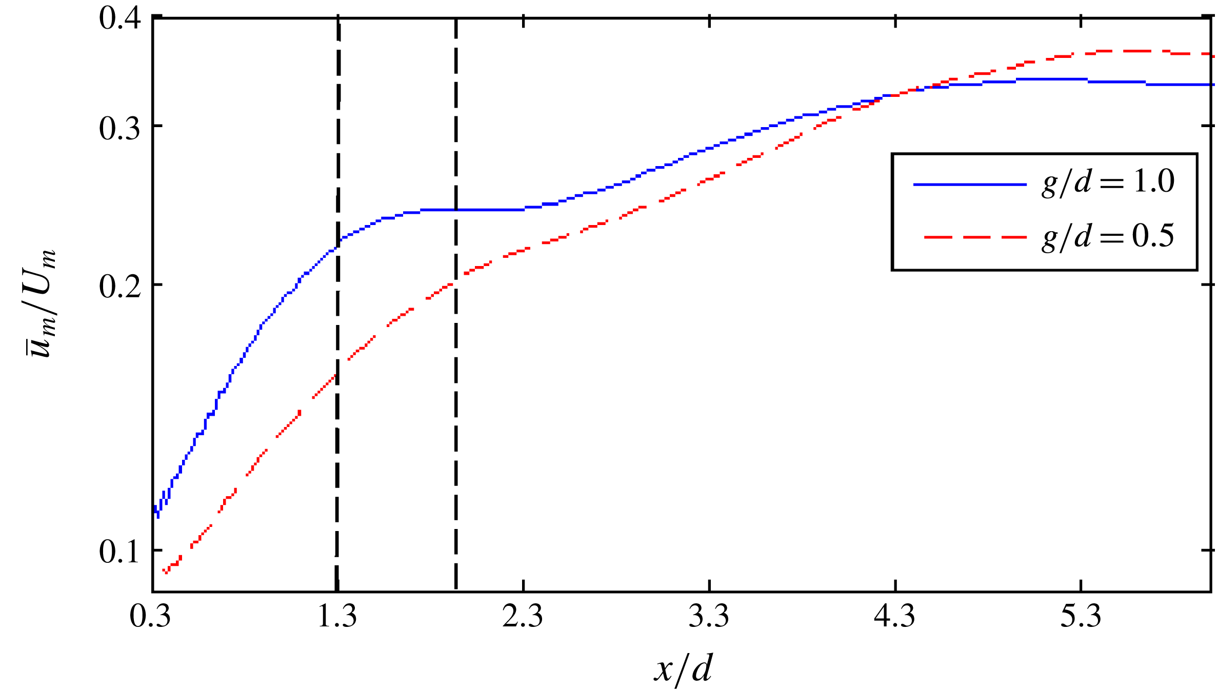
Within the framework of linear stability theory, the disturbance growth must be interpreted as a classical ‘linear growth’. One way to determine the amplitude variation of the disturbance in the separated shear layer would be to track the amplitude of the maximum fluctuation (Unal & Rockwell Reference Unal and Rockwell1988a
). The maximum level of the streamwise velocity fluctuations
 $(\bar{u}_{m})$
in the outer shear layer of the wide wake normalized by the mean streamwise velocity
 $(U_{m})$
at the edge of the shear layer is detected at various streamwise locations and shown in figure 13 for
 $g/d=0.5$
and 1.0. Regions with exponential growth of the fluctuations are seen up to about
 $x/d\approx 2$
and 1.3 for
 $g/d=0.5$
and 1.0, respectively (notice the logarithmic scaling of the vertical axis). One might therefore assume that linear stability theory can provide a reasonably accurate prediction of the instability frequency of the wide wake.
In the stability analysis of the plane mixing layer, most calculations have been conducted for the hyperbolic-tangent mean velocity profile
 $U=\bar{U}[1+\unicode[STIX]{x0394}U/(2\bar{U})\tanh (Z/2\unicode[STIX]{x1D703})]$
. Note that here, instead of using the original Cartesian coordinate axis shown in figure 1, a new
 $Z$
-axis is defined which is parallel to the main
 $z$
-axis. The origin of the new coordinate system is translated to the geometrical symmetry plane of the plate in the wide wake with its positive direction towards the outer shear layer in order to simplify the comparison between the velocity profiles in this specific wake region and the mixing-layer velocity profile.
Variation of maximum streamwise velocity fluctuations in the shear layer with respect to downstream position
 $x/d$
. The vertical axis has a logarithmic scale and the dotted lines at
 $x/d=1.3$
and 2 indicate the end of the region with exponential growth for
 $g/d=1.0$
and 0.5, respectively.

Non-dimensional mean streamwise velocity profile at different downstream positions in the immediate wake for
 $g/d=0.5$
(a) and
 $g/d=1.0$
(b). Note that the lines represent the measured mean velocity and the symbols are the hyperbolic-tangent profiles.

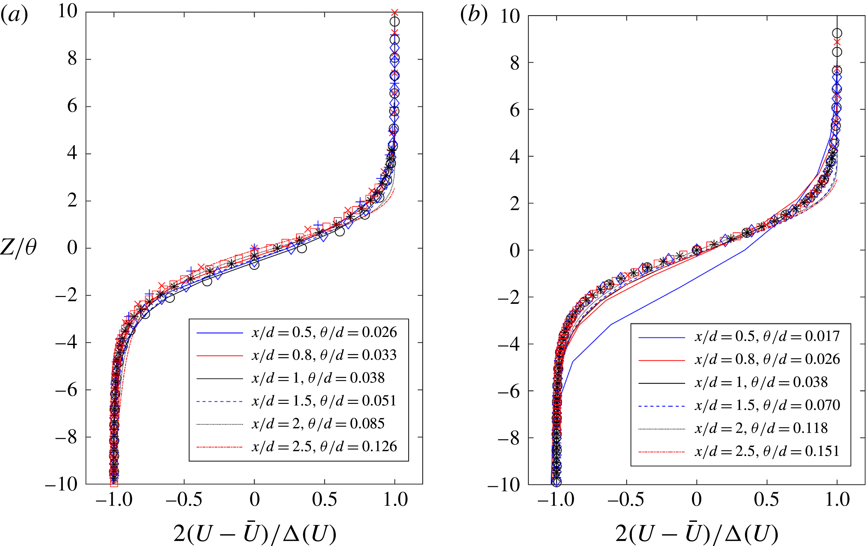
In figure 14, the variation of the non-dimensional mean streamwise velocity across the outer shear layer of the wide wakes for
 $g/d=0.5$
and 1.0 is shown together with the corresponding hyperbolic-tangent profile. Except for the first location
 $x/d=0.5$
for
 $g/d=1.0$
, the observed mean velocity profiles in the immediate wakes are very close to the hyperbolic-tangent profiles. Data for the corresponding momentum thicknesses
 $(\unicode[STIX]{x1D703}/d)$
are also provided in the figure. The momentum thickness
 $\unicode[STIX]{x1D703}$
has been calculated based on the definition for a mixing layer,
 $$\begin{eqnarray}\unicode[STIX]{x1D703}=\int _{-\infty }^{\infty }\left[\frac{1}{4}-\left(\frac{U-U_{avg}}{\unicode[STIX]{x0394}U}\right)^{2}\right]\,\text{d}Z,\end{eqnarray}$$
where
 $U$
is the mean streamwise velocity,
 $U_{avg}$
is the average velocity of the two streams and
 $\unicode[STIX]{x0394}U$
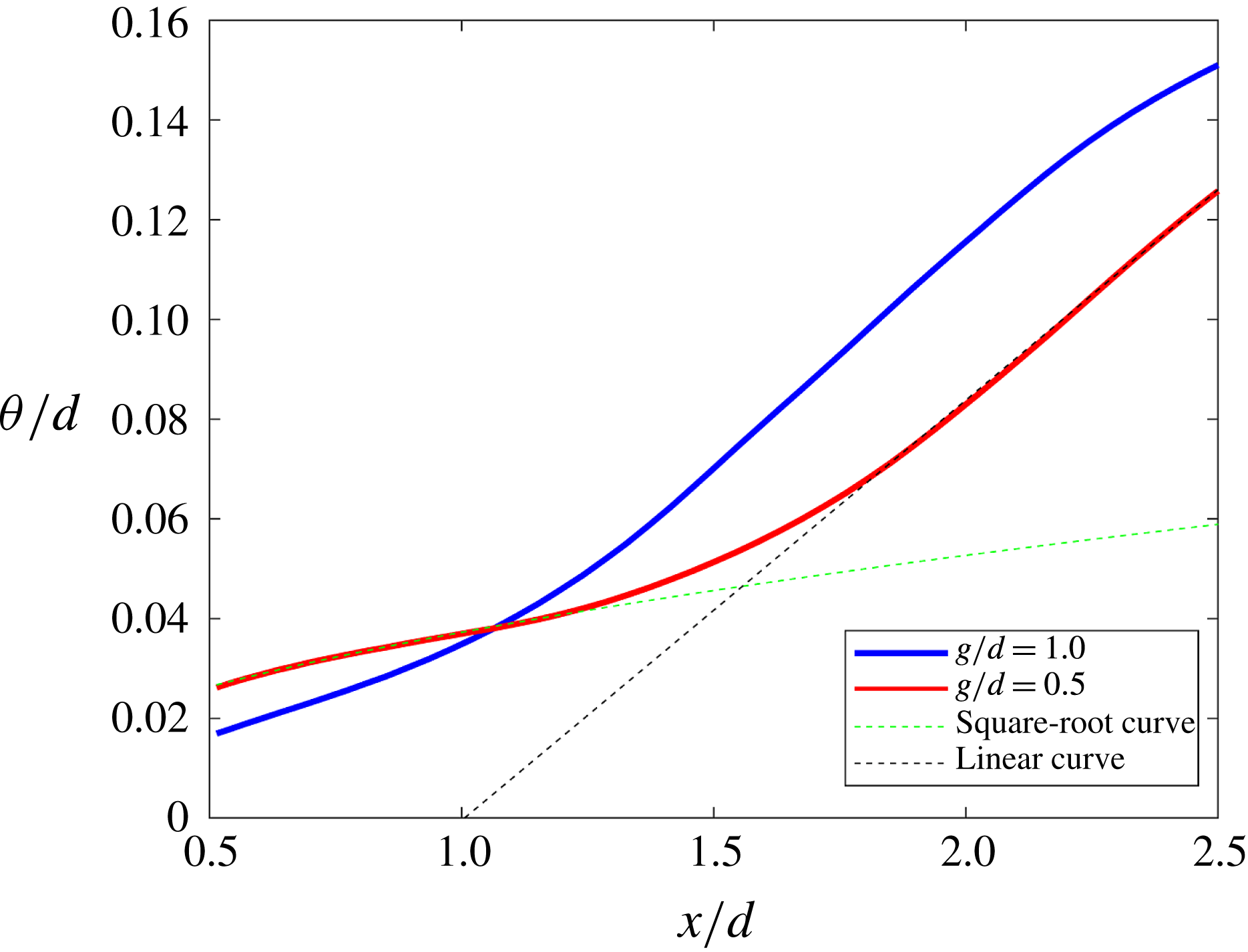
is the velocity difference between them. Here, the two flow velocities considered are the maximum flow velocity at the outer shear layer and the velocity in the base region. Figure 15 shows the momentum thickness as a function of downstream position
 $x/d$
for
 $g/d=0.5$
and 1.0. As shown by this figure, at
 $g/d=0.5$
, the momentum thickness grows as the square-root of the downstream distance up to
 $x/d=1.3$
, similarly as in the laminar region of a plane mixing layer. Further downstream, in the turbulent region, the shear layer grows linearly with the downstream distance with a growth rate
 $\text{d}\unicode[STIX]{x1D703}/\text{d}x=0.084$
. For
 $g/d=1.0$
, the momentum thickness grows linearly all the way from
 $x/d\approx 1$
and a square-root variation cannot be seen.
Momentum thickness
 $\unicode[STIX]{x1D703}$
of the separated shear layer in the wide wake for
 $g/d=0.5$
and 1.0 as a function of downstream distance
 $x/d$
. In order to estimate the two distinct growth rates of the momentum thickness at
 $g/d=0.5$
, straight dashed lines corresponding to square-root and linear growth rates are shown.

In the plane mixing layer, the Strouhal number based on linear stability theory is
 $St=f\unicode[STIX]{x1D703}/U_{avg}=0.032$
for the most amplified wave (Ho & Huerre Reference Ho and Huerre1984). Here,
 $f$
is the frequency and
 $U_{avg}$
is the average velocity across the mixing layer. One possible approach would be to assume a similar Strouhal number in the separated shear layer of the wide wake. If so, we have to choose a characteristic length in order to estimate the shear-layer instability frequency. Alternative approaches for calculating the length scale of the shear-layer instability are available in the literature, e.g. the boundary-layer thickness at the point of separation (Bloor Reference Bloor1964) and the momentum thickness at different locations along the shear layer (Wei & Smith Reference Wei and Smith1986; Unal & Rockwell Reference Unal and Rockwell1988a
; Prasad & Williamson Reference Prasad and Williamson1997).
Here, we consider the momentum thickness at the middle of the linear growth region of shear-layer instability as the characteristic length, as suggested by Unal & Rockwell (Reference Unal and Rockwell1988a
). As shown in figure 13, the
 $x$
-position of the middle of the region with an exponential growth rate is approximately
 $x/d=1$
and 0.8 for
 $g/d=0.5$
and 1.0, respectively. The momentum thickness at these
 $x$
-positions (
 $\unicode[STIX]{x1D703}_{x/d=1}=0.038$
and
 $\unicode[STIX]{x1D703}_{x/d=0.8}=0.026$
for
 $g/d=0.5$
and 1.0, respectively) is chosen as the characteristic length scale for the separated shear layer in the wide wakes. The most amplified frequency based on the linear stability theory for the plane mixing layer with similar characteristics as the separated shear layer of the wide wake (
 $U_{avg}=0.7$
and
 $U_{avg}=0.68$
for
 $g/d=0.5$
and 1.0, respectively) will be
 $f_{sl}\cong 0.59$
and
 $f_{sl}\cong 0.83$
for
 $g/d=0.5$
and 1.0, respectively.
3.2.3 Frequency analysis
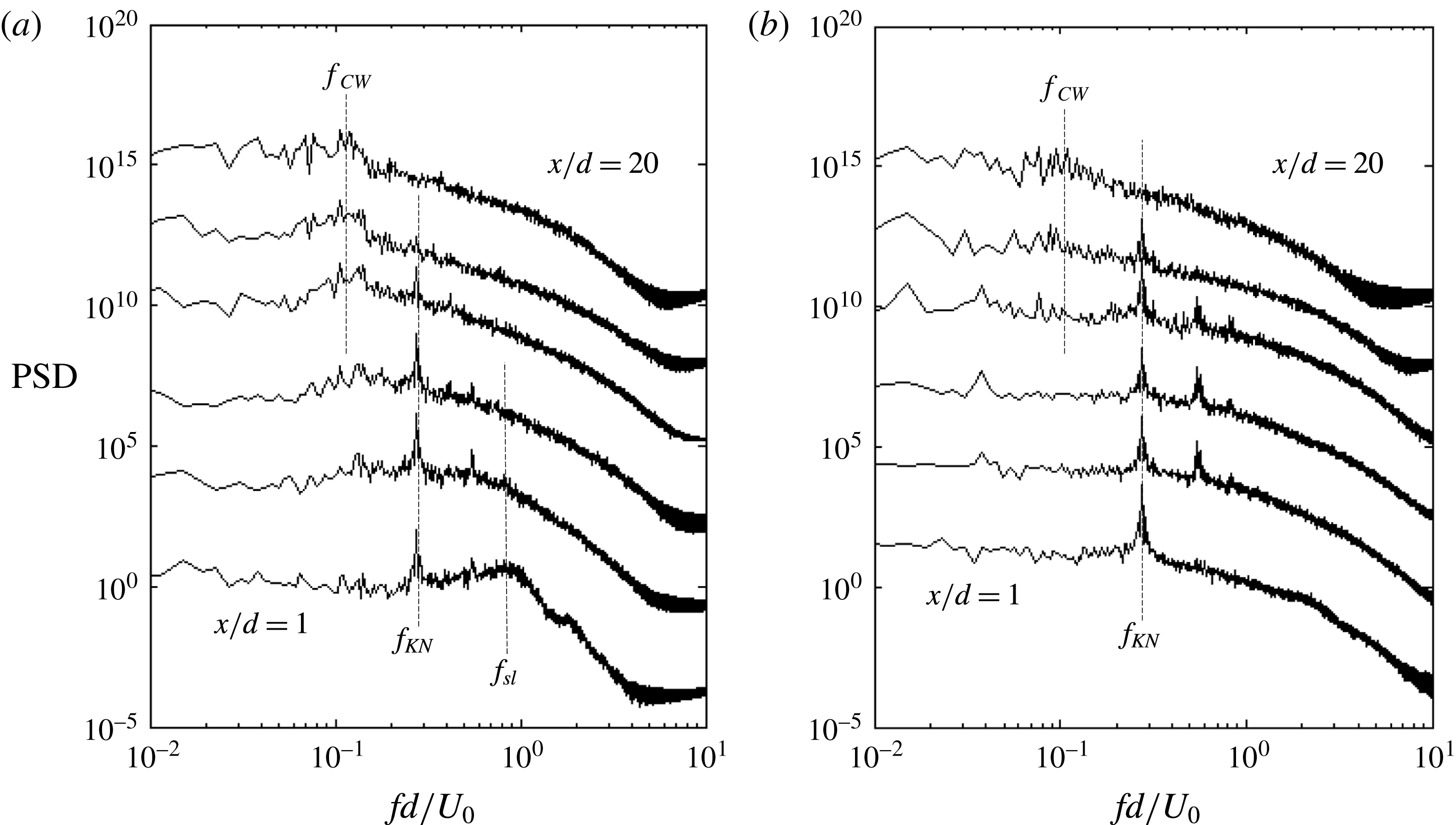
Power spectra of pressure data of (a) wide and (b) narrow wakes for
 $g/d=0.5$
, indicating the dominant frequencies at different downstream positions
 $x/d=1$
, 2, 3, 5, 10 and 20 from bottom to top, respectively. For clarity, the different spectra in (a) and (b) are offset from the first spectrum from the bottom
 $(x/d=1)$
by a factor of 1000. Therefore, only comparison between the energy density of the wide and narrow wakes at the same downstream position is meaningful.

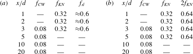
Frequency peaks in the Fourier spectra of pressure in (a) the wide wake and (b) the narrow wake, for
 $g/d=0.5$
, at different downstream positions.
In the following, power spectra taken at different downstream positions in the wide and narrow wakes are presented and the dominant frequencies corresponding to the appearance of small- and large-scale vortices are discussed. Although the frequencies in the spectra for simplicity are denoted by
 $f$
with a relevant subscript, they are non-dimensionalized as
 $fd/U_{0}$
. In order to calculate the shedding frequency, time traces of all velocity components and pressure were sampled along lines parallel to the plates at six different downstream positions from
 $1d$
to
 $20d$
within the outer sides of the narrow and wide wakes (
 $z/d$
varies from
 $\pm 1.75$
at
 $x/d=1$
to
 $\pm 3.25$
at
 $x/d=20$
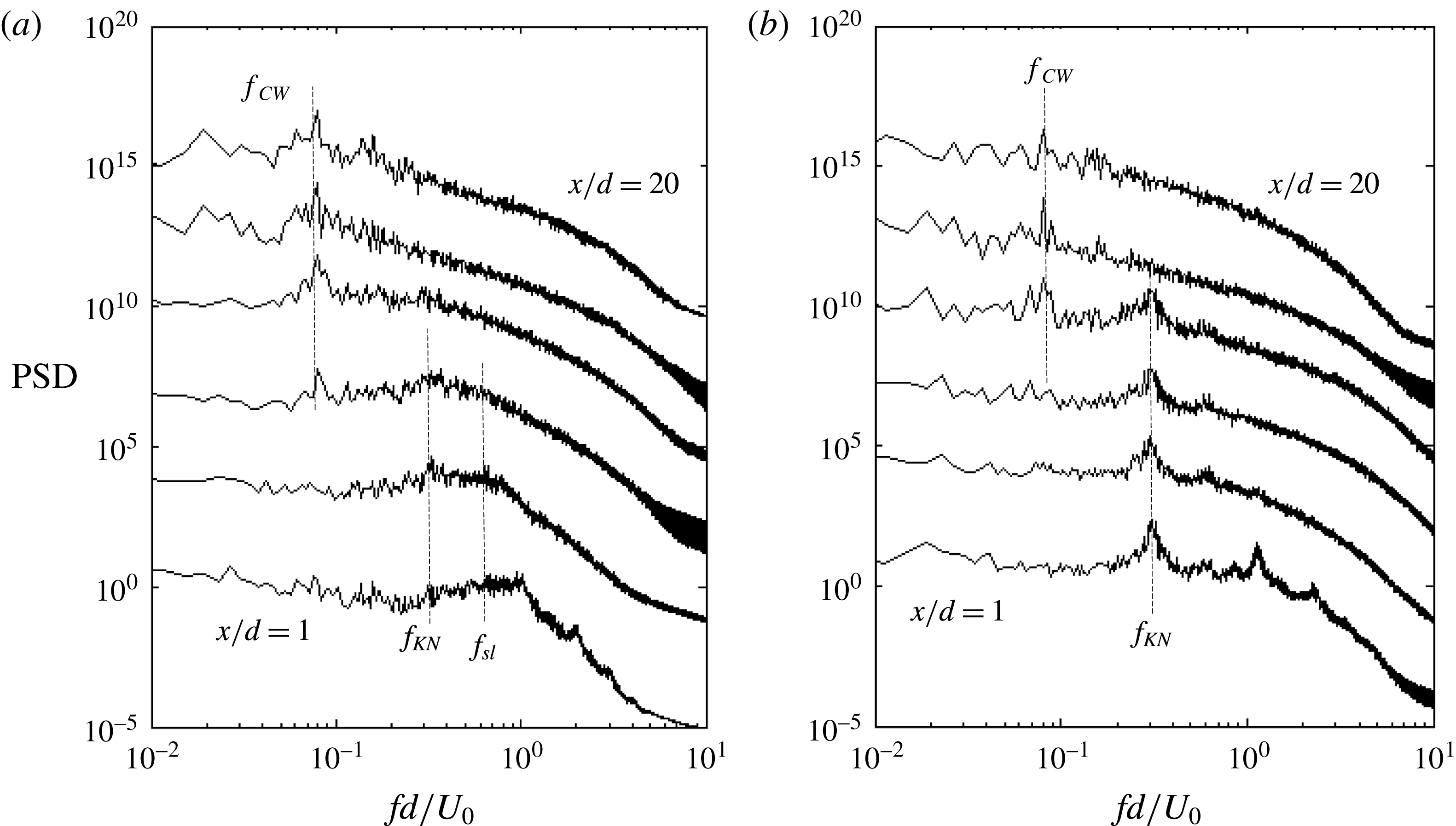
). Using fast Fourier transform (FFT) the power spectra of the velocity data are shown in figures 16 and 17, for
 $g/d=0.5$
and 1.0, respectively. The spectra were averaged over horizontal planes, i.e. in the homogenous
 $y$
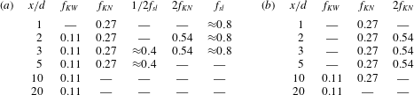
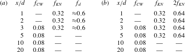
-direction. The dominant frequencies are indicated by dotted vertical lines and summarized in tables 1 and 2.
Power spectra of the wide (a) and narrow (b) wakes for
 $g/d=1.0$
, indicating the dominant frequencies at different downstream positions at
 $x/d=1$
, 2, 3, 5, 10 and 20 form bottom to top respectively. Note that the different spectra in (a,b) are offset from the first spectra from the bottom
 $(x/d=1)$
, by factors of 1000 for clarity. Therefore, only comparison between the energy density of the wide and narrow wake spectra at the same downstream position is meaningful.

Frequency peaks in the Fourier spectra of pressure in (a) the wide wake and (b) the narrow wake, for
 $g/d=1.0$
, at different downstream positions.
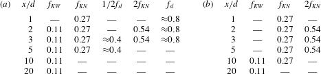
In general, the vortex shedding frequency of the narrow wake (
 $f_{KN}=0.32$
and 0.27 for
 $g/d=0.5$
and 1.0, respectively) can be observed in the near wake of the narrow and wide wakes. The passages of narrow wake shed vortices perturb the wide wake. In other words, fluctuations from the narrow wake pump into the whole domain and therefore appear in the spectra of the wide wake as well. However, the energy density corresponding to this frequency in the wide wake is much lower than in the narrow wake, especially at
 $x/d=1$
. Traces of the narrow wake in the entire flow field have been observed also by Higuchi et al. (Reference Higuchi, Lewalle and Crane1994) and Brun et al. (Reference Brun, Tenchine and Hopfinger2004).
The small peaks in the narrow wake spectra are the harmonics of the narrow wake shedding frequency. In the narrow wake, the two shear layers separated from the plate are squeezed upward due to the biased gap flow. However, due to the limited space for K–H vortices to develop and grow, it is hard to interpret the high-frequency fluctuations as a result of a K–H instability. The higher harmonics of the narrow wake frequency might be due to interactions between vortices from the different shear layers at the narrow side of the wake. In the far wake, the dominant frequency in the spectra is associated with the vortex shedding of the large combined wake,
 $f_{CW}=0.08$
and 0.11 for
 $g/d=0.5$
and 1.0, respectively.
The pressure spectra of the wide wake (figures 16
a and 17
a) exhibit a frequency associated with the Kelvin–Helmholtz instability in the separated shear layer
 $f_{sl}\approx 0.6$
and 0.8 for
 $g/d=0.5$
and 1.0, respectively. Note that the approximate positions of data sampling in the shear layers might fail to capture the shear-layer vortices all the time and accordingly lower the energy density of
 $f_{sl}$
in the spectrum, especially for
 $g/d=0.5$
at
 $x/d=1$
(figure 16
a). The higher-frequency peaks at this position correspond to higher harmonics of
 $f_{KN}$
, but disappear at locations further downstream. In the present study at
 $g/d=0.5$
, the shear-layer frequency is found to be close to the first harmonic of the narrow wake frequency and the reader may wonder if these two represent the same phenomenon. However, this frequency
 $(f_{sl})$
is also consistent with observations made from the sequence of vorticity snapshots in figure 10(a–d). The shear-layer frequencies obtained from the spectra for
 $g/d=0.5$
and 1.0 are in close agreement with the frequencies predicted by the hypothesized similarity between the separated shear layer and a plane mixing layer in § 3.2.2.
As shown by the wide wake spectra in figures 16(a) and 17(a), the low-frequency peak is absent in the immediate wake energy spectra. As discussed before, large-scale vortices do not form completely in the immediate region of the wide wake and the oscillations are dominated by a shear-layer instability. However, in the far wake, the low-frequency peak is observed in spectra both in the wide and narrow wakes. The vorticity contours in figure 10(a–d) show that the oscillations remain remarkably periodic and coherent even at large distances downstream of the side-by-side plates. This observation suggests the occurrence of an absolute or global instability. In free shear flows (such as mixing layers, jets, wakes), flow instabilities are already classified as local or global and convective or absolute depending on their dynamic behaviour (Huerre & Monkewitz Reference Huerre and Monkewitz1990). In bluff-body wakes undergoing Kármán shedding, Koch (Reference Koch1985), with the help of stability analysis, discovered the presence of local absolute instability in the near wake. However, the existence of local absolute instability may not be a sufficient condition for the amplification to global instability, but only a necessary one (Huerre & Monkewitz Reference Huerre and Monkewitz1990). The experimental findings of Mathis, Provansal & Boyer (Reference Mathis, Provansal and Boyer1984) and Strykowski (Reference Strykowski1986) further showed that low-
 $Re$
Kármán shedding is indeed a global instability. Nevertheless, the current problem involves complex wake interference effects. The problem is further contaminated by the presence of turbulence, secondary instabilities in the form of K–H waves in the separated shear layers and spanwise secondary vortices. There is some evidence in the literature that the presence of base-bleed, perforation or control cylinders in a bluff-body wake could significantly suppress the Kármán vortex shedding (Wood Reference Wood1964; Castro Reference Castro1971; Inoue Reference Inoue1985; Strykowski Reference Strykowski1986). Note that flow past a perforated flat plate (Castro Reference Castro1971; Inoue Reference Inoue1985) or a bluff body with control cylinders (Strykowski Reference Strykowski1986) is conceptually similar to the current wake flow problem, where proximity interference effects from the neighbouring wakes are dominant. In the wake of highly perforated plates (i.e. plates with larger holes and widened ‘gap’ between the solid sections), it was found that Kármán shedding is suppressed in the near wake, while the far wake exhibited a strongly periodic Kármán-like instability (Castro Reference Castro1971; Cimbala, Nagib & Roshko Reference Cimbala, Nagib and Roshko1988; Huang et al.
Reference Huang, Ferré, Kawall and Keffer1995). While Castro (Reference Castro1971) and Cimbala et al. (Reference Cimbala, Nagib and Roshko1988) attribute this to hydrodynamic instability of the mean flow, Huang et al. (Reference Huang, Ferré, Kawall and Keffer1995) propose that amalgamation of small-scale vortices in the near wake leads to the formation of this far-wake Kármán-like instability. The present vorticity fields in figure 10(a–d) indicate a similar picture (qualitatively), where the far wake is experiencing a large-scale coherent Kármán-like instability. We can draw similar interpretations as others here, where the near-wake shear-layer instabilities could be convectively unstable, while the far-wake Kármán-like structure could be an absolute or global instability.
Moreover, for
 $g/d=1.0$
in the wide wake at
 $x/d=3$
and 5 (figure 17
a) there exists a subharmonic of the shear-layer frequency. This subharmonic mode may correspond to the coalescence of the vortices similar to a plane mixing layer (e.g. Winant & Browand Reference Winant and Browand1974) and large-scale Kármán vortices form further downstream in the wide wake. Therefore, there may be a sufficiently long distance in order to enable small-scale shear-layer vortices to coalesce and the subharmonic mode to appear in the frequency spectra. Despite the fact that the spectrum indicates the existence of a subharmonic mode in the separated shear layer in the wide wake, it is not straightforward to visualize the pairing of vortices due to the formation of the large-scale Kármán vortices. Nevertheless, a pairing of vortices is visible in the snapshot of the spanwise vorticity in figure 18 at
 $tU_{0}/d=150$
. Here, the large complex vortical structure in the outer shear layer of the wide wake may be considered as a pair of transition vortices (as indicated by the supporting sketch of vortex pair).
Instantaneous spanwise vorticity
 $\unicode[STIX]{x1D714}_{y}$
at
 $y/d=1$
for
 $tU_{0}/d=150$
. Notice the sketch (in black) of a vortex pair.

3.3 Wake configuration with intermittent switching of gap flow
$(g/d=1.6)$

As mentioned in the Introduction, Brun et al. (Reference Brun, Tenchine and Hopfinger2004) studied the role of the shear-layer instability on the near-wake behaviour of side-by-side circular cylinders at
 $Re=1000{-}14\,300$
with
 $g/d=0.583$
. They suggested the appearance of the shear-layer instability as a reason that triggers the biased gap flow to switch from one side to the other. In contrast, in the case of side-by-side flat plates with
 $g/d=0.5$
and 1.0 (the asymmetric configuration) the biased gap flow turned out to be stable despite the appearance of the shear-layer instability. An additional simulation has been done for side-by-side plates with
 $g/d=1.6$
. The resulting wake switched between narrow and wide wakes and between anti-phase and in-phase vortex streets. This is consistent with observations reported by Miau et al. (Reference Miau, Wang and Chou1992, Reference Miau, Wang and Chou1996)
 $(g/d\geqslant 1.4)$
and Hayashi et al. (Reference Hayashi, Sakurai and Ohya1986)
 $(g/d=1.75)$
.
Instantaneous spanwise vorticity
 $\unicode[STIX]{x1D714}_{y}$
at the mid-plane
 $(y/d=0)$
at eight successive time instants separated 100 time units
 $d/U_{0}$
.

The present study confirms that, for side-by-side plates, the biased gap flow will be unstable at relatively larger
 $g/d$
as compared to side-by-side circular and square cylinder wakes, and furthermore, that the inception of the shear-layer instability cannot trigger switching of the direction of the gap flow. Figure 19 shows instantaneous spanwise vorticity contours at eight different time instants. The time interval between the snapshots is
 $100d/U_{0}$
. In panel (a) two anti-phase vortex streets are symmetric about the gap axis. Later on in panel (b) the symmetry no longer exists and in panel (c) a biased gap flow with wide and narrow wakes is observed behind the upper and lower plates, respectively. In panel (d) the two vortex streets shed in phase from the side-by-side plates. Afterwards, in panel (e), the biased gap flow resulted in wide and narrow wakes. In the next snapshot (f), a symmetric configuration of the vortex streets (with anti-phase shedding), similar to that in panel (a), occurs. Next, we observe in (g) narrow and wide wakes behind the upper and lower plates, respectively. Finally, in the last snapshot (h), narrow and wide wakes switch to the lower and upper sides of the wake, respectively. In the present manuscript, only a qualitative presentation of the flip-flopping is provided. A statistical characterization of the phenomenon is beyond the scope of this already lengthy paper.
4 Conclusion
Wakes behind two side-by-side flat plates have been investigated by means of three-dimensional computer simulations at moderate
 $Re$
. Direct numerical simulations (DNS) were performed for
 $g/d=0.5$
, 1.0 and 1.6 at
 $Re=1000$
based on the plate width
 $d$
.
Two qualitatively different wake configurations were found in the present study for
 $g/d=1.0$
. Depending on the initialization of the computations, either a symmetric or an asymmetric wake configuration resulted from the simulations and both wake configurations turned out to be stable after being established. For the same
 $g/d$
, but at
 $Re=1500$
, Higuchi et al. (Reference Higuchi, Lewalle and Crane1994) initially observed a symmetric wake as the tunnel flow was started from rest in their experiments, but the wake turned asymmetric within a time span of several vortex shedding periods. However, in the higher-
 $Re$
experiment
 $(Re=8000)$
with
 $g/d=1.0$
, only an asymmetric wake configuration was observed by Miau et al. (Reference Miau, Wang and Chou1992). From the present study we find that either a symmetric or an asymmetric wake configuration can result from computer simulations for exactly the same parameter values (
 $g/d$
and
 $Re$
) and moreover that either configuration is persistent after first having been established.
In the symmetric wake configuration of the present study, two anti-phase Kármán vortex streets can be distinguished in the near wake, but they merge and form a large single wake further downstream. Surprisingly, two different three-dimensional instability features were observed in the upper and lower wakes: one with spanwise wavelength
 $2d$
and period-doubling characteristics similar to mode C, and the other one with a shorter spanwise wavelength
 $({\sim}1d)$
and a mushroom-like pattern in the cross-sectional view, which resembles the mode B instability. These results suggest that a possible state may arise in the wake behind two side-by-side flat plates with a combination of two qualitatively different three-dimensional instability features. This might be the result of nonlinear interactions between the two wakes at this particular
 $Re$
and
 $g/d$
. A possible scenario for the physical mechanism of the coexistence of two different instability features was discussed in terms of Biot–Savart induction.
The asymmetric wake configuration observed for
 $g/d=1.0$
resembled the narrow and wide wakes for
 $g/d=0.5$
. The narrow wake exhibited strong alternating vortex shedding, whereas no periodic shedding was observed in the immediate part of the wide wake. However, shear-layer transition vortices were detected, apparently for the first time in the wide wake behind side-by-side plates. A hypothesized analogy between the separated shear layer in the wide wake and a plane mixing layer was supported by the DNS data. The shear-layer frequency (
 $f_{sl}\sim 0.6$
and 0.8 for
 $g/d=0.5$
and 1.0, respectively) was in good agreement with the frequency calculated based on linear stability theory for a mixing layer, thereby giving further support to the analogy.
Finally, the wake behind the side-by-side plate configuration with
 $g/d=1.6$
was examined and the resulting flow exhibited a flip-flopping phenomenon. This finding suggests that the biased gap flow behind side-by-side plates becomes unstable at a relatively larger
 $g/d$
than earlier reported for side-by-side circular and square cylinder wakes. We can furthermore conclude that the inception of the shear-layer instability cannot trigger a switching of the direction of the gap flow.
The wealth of detailed information that can be extracted from carefully designed and controlled computer experiments of complex wake flows supplements laboratory measurements and may aid resolution of apparently contradictory observations.
Acknowledgements
This work has received support from The Research Council of Norway (Program for Supercomputing) through a grant of computing time. The first author is the recipient of a research fellowship offered by The Research Council of Norway.