Introduction

The marginal ice zone (MIZ) around Antarctica is that region of broken floes and pack ice surrounding the continent during winter and spring in which the ocean wave behaviour is distinctly modified from that in the open sea. The striking feature of the surface and waves on entering the MIZ is that the average floe size increases as the wave field becomes smoother than the open sea. This simultaneous lengthening of the dominant wavelength and lengthening of the mean floe size away from the open sea is evidence of the feedback nature of the wave-ice interaction in the MIZ. That interaction involves the bending of floes by ocean waves, with breaking resulting particularly for those wavelengths that lead to large floe flexure, and the concomitant scattering of wave energy. Loss of wave energy also occurs through mechanisms such as wave sloshing around floes and collisions between floes. Thus the wave field modifies the floe-size distribution while the presence of floes simultaneously modifies the wave field.

This paper focuses on the part of the interaction that involves the scattering of surface ocean waves by floes within the MIZ, and in particular establishes a field measurement of the dispersion relation −being the relationship between frequency and wave number- for surface-gravity waves propagating within the Antarctic MIZ. This measurement can then be used to calibrate or validate models for wave scattering in the MIZ which typically produce a prediction of group speed as a function of frequency.

A number of models for scattering in the MIZ have recently been developed. Reference Dixon and SquireDixon and Squire (2000a) used the well-established theory of random media to develop an effective medium approach, using the coherent-potential approximation to derive a dispersion relation for propagation within a plate of ice with random scattering inclusions. Such models predict the mean-free path for energy propagation between scatterers, which sets the boundary between primarily coherent transport and totally diffusive transport. That work is presently being extended to include the effect of the water to give a model for scattering in the MIZ (Reference Dixon, Squire, Pullan and RyanDixon and Squire 2000b). Reference Meylan, Fox, Chung, Sayed, Hobbs and YoergerMeylan and Fox (1996) developed a semi-empirical model using the scattering from a single floe to give the scattering kernel in a linear Boltzmann equation describing the propagation and scattering of wave intensity. Steady-state solutions were presented by Reference Meylan, Squire and FoxMeylan and others (1997). Reference Meylan, Pullan and RyanMeylan (2000) has improved the estimate of the scattering kernel by taking into account the local coherent effects between floes to calculate the mean intensity scattering for square floes averaged over floe position and orientation for a given mean floe size and separation. Both these models result in a Boltzmann-type transport equation for wave intensity. Solutions lead to the effective group speed as a function of frequency in the scattering medium, which is the derivative of the effective dispersion equation in the composite medium.

Dispersion Relations and Wave Speed

Surface ocean waves of small amplitude-or of moderate amplitudes where cresting does not occur - are made up of plane propagating waves that have the form (the real part of)

where x and t are the horizontal space and time coordinates, respectively, and k and ω are the vector wavenumber and radial frequency of the wave. The wave propagates in the direction given by the unit vector k/k, where k = ||k|| is the magnitude of the wavenumber. The wavelength is therefore A = 2π/k and the period is T = 2π/ω.

In a given medium there is a functional relation between period and wavelength, usually stated as the relation between magnitude of the wavenumber and radial frequency, called the dispersion relation. Wave propagation in homogeneous media has a well-defined dispersion relation, while the effective dispersion relations for inhomogeneous media depend on the scale being observed. Our interest here is in making a measure of the dispersion relation for propagating waves in the Antarctic MIZ and seeing whether it conforms to one of the simple dispersion relations for a homogeneous medium or whether the inhomogeneity of the ice field is important.

When the ice floes have no effect on wave propagation, as occurs in the long-wavelength limit, the dispersion relation is just that for the open sea, which is (assuming deep water)

At long wavelengths, though not necessarily in the limit, the surface cover of broken floes affects the wave propagation because of the added mass at the surface compared to open water. If the rigidity of the floes or viscous effects have no role, then the dispersion relation becomes

where d_s is the specific density of sea ice (which is close to 1) and h is the thickness of the ice cover. If the ice cover is homogeneous, in that all floes have the same thickness, then the value of h, and hence the dispersion relation, is well defined. Otherwise, an effective value for h is required, which typically depends on the scale being observed. When the frequency is low enough that ω² ≪ g/ch, then the added-mass dispersion relation reduces to the dispersion relation for open water, so k ∝ ω ² , and we can conclude that the mass of the floes has no effect on wave propagation. Above that frequency the added mass increases the wavenumber and hence reduces the wavelength for a given frequency, though this effect is small for typical ice thicknesses and periods. At the higher frequencies where the added mass is appreciable, typically the flexural rigidity of the floes becomes important - for ice-floe sizes and thicknesses of geophysical interest. Then the dispersion relation for a homogeneous ice sheet with flexural rigidity L is between the positive real root k of

and the radial frequency ω Here p is the density of sea water. It can be shown that the radial frequency ωc = (pg ⁵/L)^1/8 sets a transition in behaviour of this dispersion equation. For ω < ωc, k ≈ ω ²/g as for open water , while for ω > ωc, k ≈ (pω ²/L)^1/5, i.e. k α ω ^2/5.

The dispersion relation completely characterizes the propagation of waves and energy in a (linear) medium. For example, the ratio of wavelength over period gives the phase speed

which is the speed of propagation of peaks or troughs in a monochromatic wave. In open water this speed is (using Equation (1)) cp(ω) = g/ω, so phase speed is inversely proportional to frequency. When the phase speed is not constant with frequency, the waves of different frequency that make up a wave packet will propagate with differing phase speeds and the packet will disperse, hence the name of the relation. For packets with a relatively narrow bandwidth, the envelope of the wave packet and hence the energy in the wave packet propagates with the group speed

So a wave packet in the open sea propagates with speed Cg(ω) = g/2ω when the central frequency of the packet is ω, i.e. half the phase speed.

A topic of current research is development of models for wave propagation in the MIZ that take into account the inhomogeneous nature of the ice cover that leads to wave scattering and other phenomena. These models predict the effective wave speeds or, equivalently, the effective dispersion relation. In this paper we present an experimental measurement of the dispersion equation in the Antarctic MIZ for comparison with the predictions of the simple models above, or the more complicated models that include scattering, etc.

Description of Measurements

Measurements of the wave field in the Antarctic MIZ were made on 11 June 1998 during cruise NBP 98−3. For that cruise, research vessel Nathaniel B. Palmer was taken into the pack ice southwards on longitudes 180° to the Ross Ice Shelf and then northwards on longitudes 175° E and 175° W The measurements reported here were taken at position 65°40’S, 174°56’W, which was inside the pack ice about 10 km from the open sea.

Figure 1 shows a snapshot of the radar screen taken during the measurements. The wave field is quite clearly visible, and is dominated by long-crested waves propagating from the open sea. The direction of wave propagation, estimated from this picture, is from 305°. The important conclusion is that measurements of wave height, or acceleration, made at two points in the wave field that are close enough to experience coherent wave fields, will suffice to measure the dispersion relation.

Fig. 1.

The ship’s radar screen at the time of the measurements. North is upwards. wave crests due to waves from bearing 305° are visible.

Two ice floes were instrumented, each with a global positioning system unit that recorded the floe’s position each second and accelerometers that measured the vertical and horizontal accelerations every 0.1s. Each floe was roughly oval in shape, floe 1 being 7 m × 4.4 m and 0.3 m thick, while floe 2 was 9.0 m × 6.2 m and 0.6 m thick. Figure 2 shows the instrumentation being deployed on one of the ice floes. The ship then stood away from the floes (about 10 km), and the floe data were telemetered to the ship and recorded in digital form. The two floes were separated by a distance of about 250 m during the recording period (though approximately 150 m in the direction of propagation), and hence they experienced different wave motions. Figure 3 shows a trace of the position of floe 2 with respect to floe 1, for the duration of measurements. At the start of the measurement period, floe 2 was positioned −27 m east and 191 m north relative to floe 1.

Fig. 2.

Deploying the instrumentation on an ice floe from a basket lowered over the side of the ship.

Fig. 3.

The position of floe 2 with respect to floe 1, shown for the 3000 s of the data that are analyzed.

We analyze a section of those data recorded between 0630 and 0721 GMT, i.e. nearly 50 min duration. Figure 4 shows a 500 s section of the record of accelerations, offset vertically for clarity. The wave structure is clearly visible in the vertical acceleration. Note that the horizontal accelerations are much smaller than the vertical motion, but do contain occasional spikes that are probably the result of collisions between floes.

Fig. 4.

A typical record of measured accelerations. The upper trace is vertical acceleration, while the lower, smaller-amplitude, traces give the acceleration in perpendicular horizontal directions. The traces have been offset for clarity, so the mean level should be ignored.

The power spectral density (PSD) for vertical acceleration during the 50 min record is shown in Figure 5. This estimate was found using Welch’s method (Reference WelchWelch, 1967) by segmenting the record into sections of length 4096 (409.6 seconds), windowing with a Hanning window, taking Fourier transforms and then averaging the square magnitude of the transforms. Hence the averaged frequency bins have width 1/409.6 = 0.0024 Hz. The resulting estimate is scaled so that the integral of the square of the signal equals the integral of the PSD. This estimate achieves variance reduction by effectively smoothing over frequencies. Note that the wave energy is limited to the frequencies 0.05 < / < 0.15, corresponding to periods of 6.5−20 s.

Fig. 5.

PSD for vertical acceleration of the two floes. Floe 1: solid line; floe 2: dashed line.

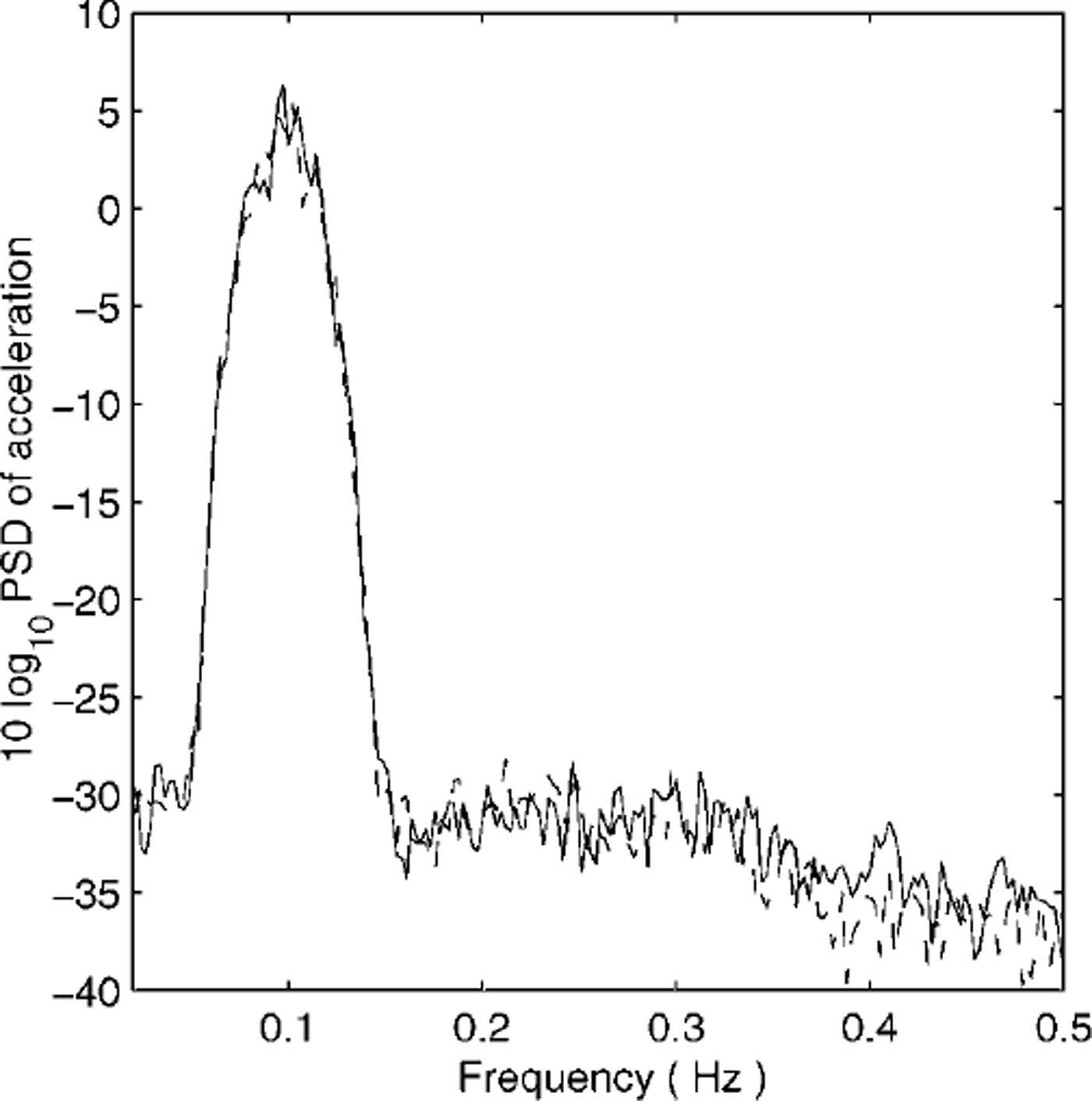
The dispersion equation is estimated by measuring the phase difference between vertical accelerations at the two floes and using the separation between floes, in the direction of wave propagation, to obtain the phase speed. This simple scheme is complicated by the floes moving in the pack and with respect to each other during the measurement (Fig. 3).

Estimating the Dispersion Relation

The estimate of the dispersion equation is made by fitting the implied transfer function that holds between the vertical acceleration of the two floes. Because the wave field is dominated by waves propagating in a single direction, the transfer function at frequency w is then given by

where ΔX is the distance between the floes in the direction of propagation. The term a(ω) is due to the degree of correlation, or equivalents the angular spread, of the wave field. It would equal 1 for perfectly unidirectional wave fields, though it is typically < 1.

We denote the vertical acceleration at floes 1 and 2 by _z1(t) and z2(t), respectively, and the Fourier transforms of these time series by z1(ω) and z2(ω), respectively. Assuming the transfer function s(ω) is constant over a band of frequencies ω ∊ t, the transfer function from floe 1 to floe 2 can be estimated by the generalization of Welch’s method

Note that the denominator in this estimate is the PSD at floe 1. The integral over frequencies in the numerator cannot be achieved by averaging over segments, as in Welch’s method, because the transfer function changes with time as the separation of the two floes changes. Instead, we generalize Welch’s method and fit a transfer function of the form in Equation (6) to the sequence of estimates calculated for each time segment. If the distance between floes ax remained constant, this fitting procedure would reduce to the estimate in Equation (7). The resulting magnitude of wavenumbers is shown with dots in Figure 6.

Fig. 6.

Measured dispersion relation (dots) along with open-water dispersion relation (dotted line) and best-fit power law (dashed line).

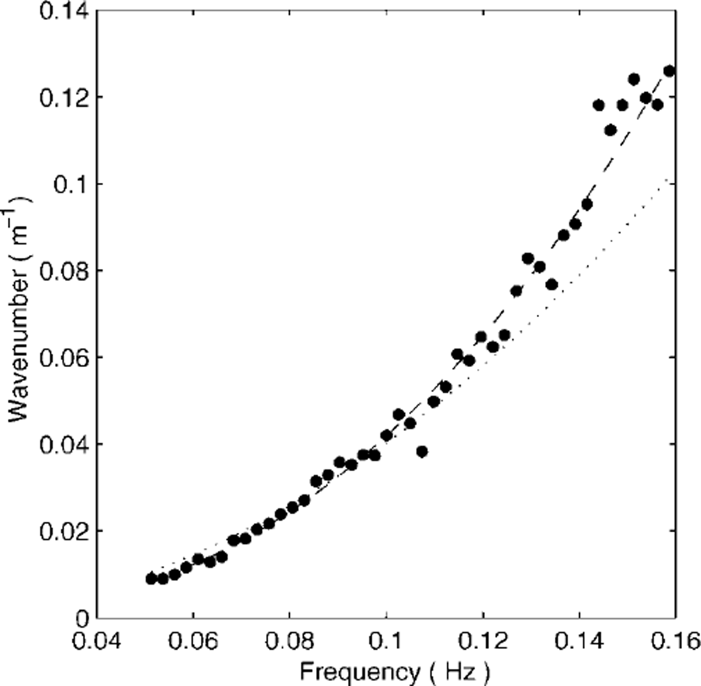
The dispersion relation for open water is also shown in Figure 6 (dotted line). It is clear that the measured wavenumber values are consistently larger (shorter wavelength) than those given by the open-water relation, for frequencies above 0.1 Hz. The best-fit power law is shown as a dashed line and gives k ∝ ω_2.41. This exponent is significantly different to the exponent 2 in the open-water model, and also does not fit the dispersion relations given earlier. Given that the measured dispersion relation fits the power 2.41 well, it seems clear that a systematic effect is occurring. Possible causes of this effect are that the bobbing response of the floes is different and introduces a systematic phase effect, or that the directionality of the wave field causes a drop-off in correlation with frequency, leading to a systematic bias in our estimate. However, both these explanations are unlikely since the bobbing frequency is much greater than the wave frequencies of interest here, while the coherence effect would introduce noise in the estimates which is not evident in Figure 6. Another possibility is that the dispersion relation in the MIZ is significantly affected by the presence of the pack ice and is different to that in open water.

The fitted dispersion equation crosses the open-water dispersion equation close to the frequency / = 0.1 Hz. At that frequency the phase velocities are equal since, for both open water and the MIZ, ω/k = 2π × 0.1/0.04 = 16 ms^-1. Since the measured wavenumber is slightly smaller than the open-water wavenumber for / < 0.1 , the phase velocity in the MIZ is slightly greater than the phase velocity in open water at low frequencies. Conversely for / > 0 . 1 the measured wavenumber is significantly larger than the open-water wavenumber, and hence the actual phase velocity is substantially less than that in open water. This suggests that at shorter periods, waves in the MIZ do not behave like gravity waves and that some other mechanism is more important in defining the wave velocity.

Conclusions

We conclude that it is possible to measure the actual dispersion relation in the Antarctic MIZ using the motion of two floes, at least under the assumption of a unidirectional wave field. The spacing between floes cannot be completely determined, as it depends on the motion of the pack ice. However, we used a dataset in which the separation between floes in the direction of propagation is close to one wavelength at the dominant frequency of 0.1 Hz. That spacing provides a good compromise between the greater coherency with smaller floe spacing as opposed to greater calculation accuracy at larger spacing. The precise spacing that is optimal depends on the details of directivity in the wave field, with more coherent wave fields allowing greater spacing and hence accuracy. However, it seems unlikely that much more than one wavelength spacing is ever necessary. Note, however, that the method given here may be generalized to analyze the vertical motion of many floes to give the directionality of the wave field as well as the dispersion relation. That measurement would overcome the difficulties associated with using just two floes. The measured dispersion relation proved to be significantly different to the relation for open water. While the added-mass and ice-sheet models predict dispersion equations with power laws <2, we found that the measured dispersion equation has a power law with exponent >2. The possible causes and mechanisms for this measured power law are certain to provide a focus for future research.