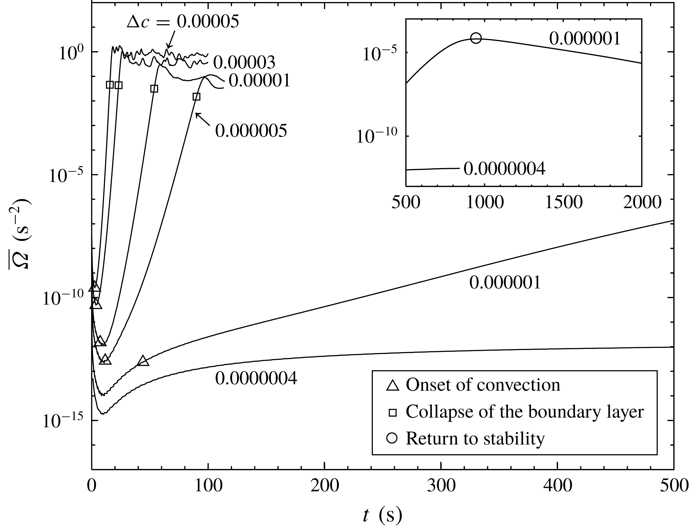
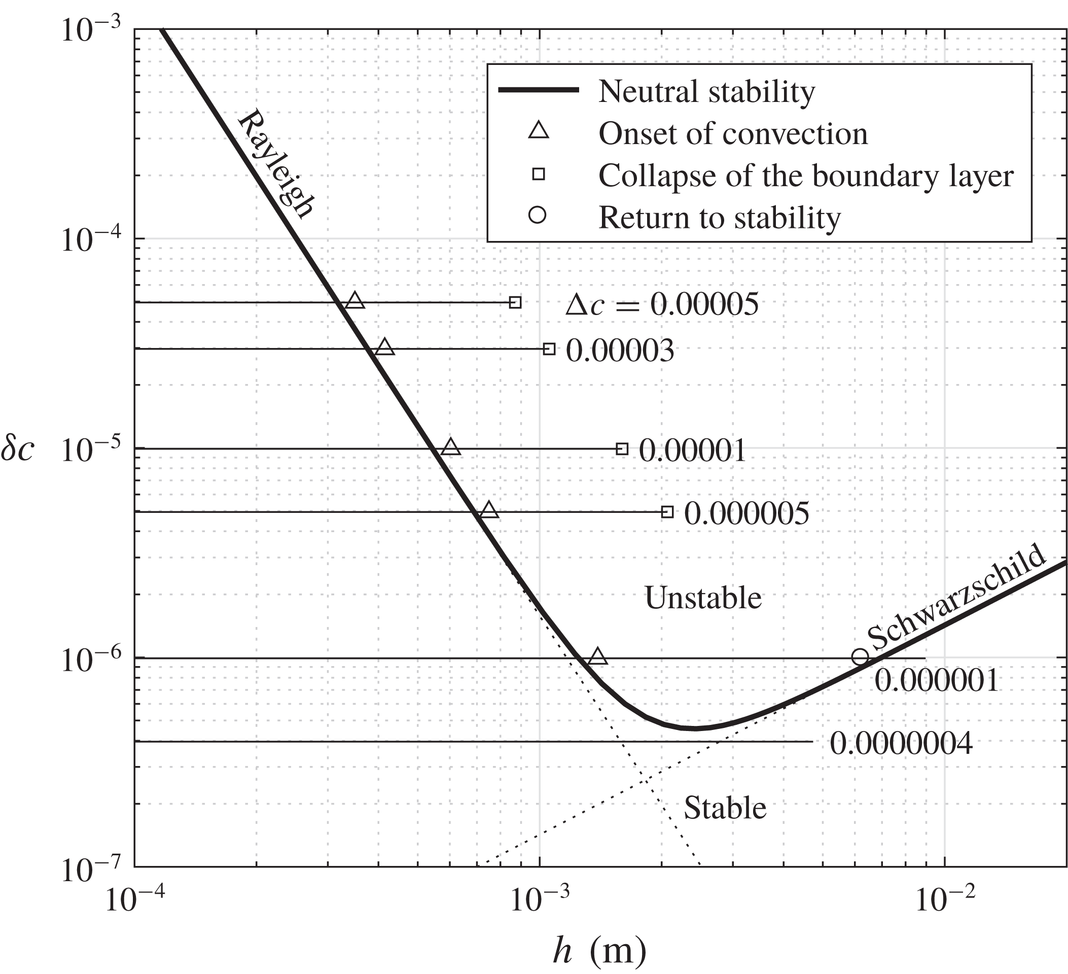
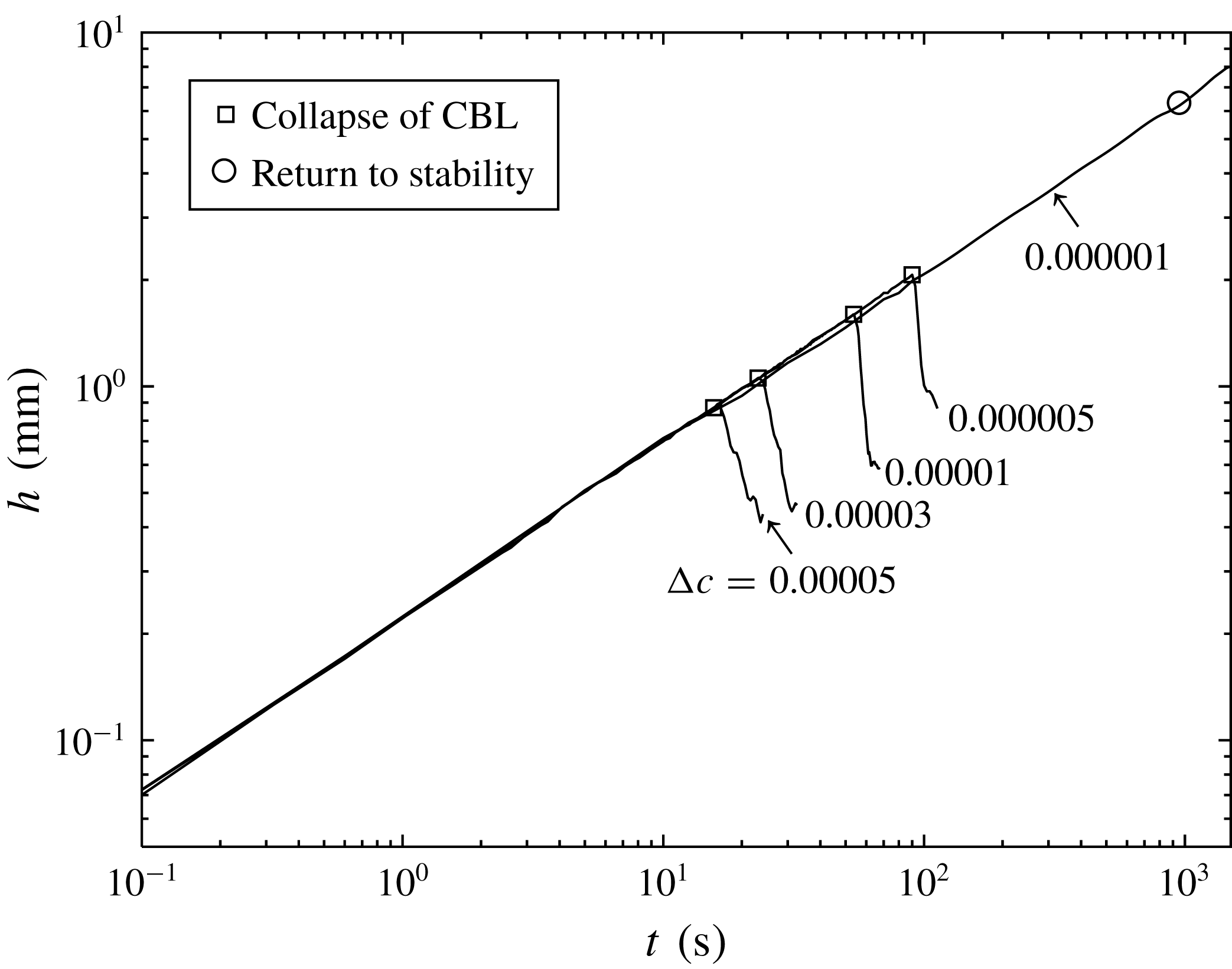
1 Introduction
As the gas–liquid critical point is approached, strong anomalies can be found in the thermodynamic and transport coefficients of a pure fluid (Zappoli Reference Zappoli2003; Carlès Reference Carlès2010). In particular, both the isothermal compressibility and the thermal expansion coefficient grow dramatically while the thermal diffusivity tends to zero. The hyper-compressible and low heat-diffusing nature of near-critical pure fluids results in a special coupling process between thermal equilibrium and mechanical disturbance, known as the piston effect (PE). Owing to buoyant convection on Earth, the PE had long been ignored and was first observed in a micro-gravity experiment conducted by Nitsche & Straub (Reference Nitsche and Straub1987). Then the mechanism of the PE was revealed (Boukari et al. Reference Boukari, Shaumeyer, Briggs and Gammon1990; Onuki, Hao & Ferrell Reference Onuki, Hao and Ferrell1990; Zappoli et al. Reference Zappoli, Bailly, Garrabos, Le, Guenoun and Beysens1990): when a near-critical fluid is subjected to boundary heating, a very expandable, thin, diffusive layer forms, which compresses the bulk fluid and causes the temperature of the bulk fluid to increase in a fast and homogeneous manner. Asymptotic expansions were employed to study the relaxations of temperature and density fields (Zappoli & Carlès Reference Zappoli and Carlès1995; Bailly & Zappoli Reference Bailly and Zappoli2000). Meanwhile, several experimental studies were carried out to evidence the PE (Guenoun et al. Reference Guenoun, Khalil, Beysens, Garrabos, Kammoun, Le Neindre and Zappoli1993; Straub, Eicher & Haupt Reference Straub, Eicher and Haupt1995; Zhong & Meyer Reference Zhong and Meyer1995; Garrabos et al. Reference Garrabos, Bonetti, Beysens, Perrot, Fröhlich, Carlès and Zappoli1998).
The above studies concerning the PE exclude its interplay with gravity. In fact, the strong compressibility makes a near-critical pure fluid sensitive to even negligible temperature variations. Under the effect of gravity, natural convection usually occurs in the fluid unless heat is applied from the top. In the past 20 years, many efforts have been made to investigate natural convection in near-critical pure fluids, with an emphasis on its interaction with the PE and the criterion for convection onset. Considerable attention has been paid to the Rayleigh–Bénard (RB) problem, where a near-critical fluid is confined between two isothermal plates separated by a distance
 $L$
heated from below. It shows that the relaxation of the temperature field is still dominated by the PE, on a time scale much faster than that of convection. As a result, the temperature distribution exhibits unique characteristics, including temperature rising homogeneously in the bulk that is enclosed by two thermal boundary layers of thickness
 $\unicode[STIX]{x1D6FF}$
, cold at the top and hot at the bottom (Amiroudine et al.
Reference Amiroudine, Bontoux, Larroud, Gilly and Zappoli2001). If the temperature difference is large enough, the boundary layers become unstable and convection then occurs. For the hot boundary layer, the problem corresponds to the RB instability for a fluid layer with a thickness
 $\unicode[STIX]{x1D6FF}$
.
The theoretical analyses of Giterman & Shteinberg (Reference Giterman and Shteinberg1970) and Carlès & Ugurtas (Reference Carlès and Ugurtas1999) revealed that, for near-critical RB instability, the onset of convection is predicted by an unusual criterion that takes into account two classical terms. The first term corresponds to the Rayleigh criterion that is derived from the Boussinesq approximation where the compressibility of the fluid is neglected. The Rayleigh criterion, considering the competition between buoyancy and viscosity, is valid for incompressible fluids or normally compressible fluids at small space scale. The second term corresponds to the Schwarzschild criterion (adiabatic temperature gradient criterion), which usually works at large atmospheric scale where the stabilizing effect of the hydrostatic pressure is prominent. Indeed, the involvement of the Schwarzschild criterion at small space scale is caused by the appreciable density stratification due to the divergent isothermal compressibility. The resulting Rayleigh criterion is given by (Carlès & Ugurtas Reference Carlès and Ugurtas1999)
 $$\begin{eqnarray}R={\displaystyle \frac{\unicode[STIX]{x1D70C}g\unicode[STIX]{x1D6FD}(\unicode[STIX]{x1D735}_{T}-\unicode[STIX]{x1D735}_{ad})L^{4}}{\unicode[STIX]{x1D702}D_{T}}}\geqslant R^{cri},\end{eqnarray}$$
where
 $R$
is the modified Rayleigh number (based on the departure of the temperature gradient from the adiabatic gradient);
 $\unicode[STIX]{x1D70C}$
,
 $g$
,
 $\unicode[STIX]{x1D6FD}$
,
 $D_{T}$
and
 $\unicode[STIX]{x1D702}$
are the density, gravitational acceleration, thermal expansion coefficient, thermal diffusivity and dynamic viscosity, respectively;
 $\unicode[STIX]{x1D735}_{T}$
is the negative temperature gradient in the fluid layer;
 $\unicode[STIX]{x1D735}_{ad}$
is the adiabatic temperature gradient; and
 $R^{cri}$
is the critical Rayleigh number, which is equal to 657.5, 1707.8 or 1100.6 depending on whether the upper and lower boundaries are both stress-free, both solid and isothermal, or one boundary is solid and the other is stress-free, respectively (Chandrasekhar Reference Chandrasekhar1961). The above criterion has been proven experimentally by Kogan, Murphy & Meyer (Reference Kogan, Murphy and Meyer1999), Kogan & Meyer (Reference Kogan and Meyer2001) and Meyer & Kogan (Reference Meyer and Kogan2002) and numerically by Amiroudine et al. (Reference Amiroudine, Bontoux, Larroud, Gilly and Zappoli2001) and Accary et al. (Reference Accary, Raspo, Bontoux and Zappoli2005b
). Besides, a return to stability according to the Schwarzschild criterion has been evidenced by numerical simulations (Accary et al.
Reference Accary, Raspo, Bontoux and Zappoli2005c
). A three-dimensional direct numerical simulation has been preformed by Accary, Bontoux & Zappoli (Reference Accary, Bontoux and Zappoli2009) elaborating the convection from its onset to steady state.
It is well known that the non-uniformity in concentration of a multicomponent fluid system also causes the non-uniformity in density, which may further contribute to the buoyancy-driven natural convection. There is a wide interest in natural convection driven by a concentration gradient in the natural environment and industrial processes, such as that caused by non-uniformity of humidity in air and in buildings, and that caused by non-uniformity of salinity in seawater (Ghiaasiaan Reference Ghiaasiaan2011). Besides, natural convection caused by combined thermal and mass gradients is also a common phenomenon that draws extensive attention (e.g. Trevisan & Bejan Reference Trevisan and Bejan1987; Weaver & Viskanta Reference Weaver and Viskanta1991a ). Such a problem becomes more interesting and challenging when two inter-diffusion mechanisms, Soret and Dufour effects, take part (Weaver & Viskanta Reference Weaver and Viskanta1991b ). However, most of the related studies in this field pay attention to general incompressible fluids, for which the Boussinesq approximation holds. There is no study concerning concentration-induced natural convection in a multicomponent near-critical fluid system. Even though one of the most important engineering applications of near-critical and supercritical fluids is chemical extraction, where multicomponent fluids are always involved, this topic has not received the attention it deserves. In fact, similar to pure fluids, the physical properties of a near-critical binary fluid mixture also exhibit singularities, especially when it is dilute. For example, the compressibility is strong, the diffusion coefficient vanishes at the critical point because of the sharp clustering phenomenon (Vaz, Magalhães & Silva Reference Vaz, Magalhães and Silva2014), and the partial molar volume becomes large (Sengers Reference Sengers1994; Luettmer-Strathmann Reference Luettmer-Strathmann2002). It is reasonable to believe that the natural convection in a near-critical binary fluid mixture induced by a concentration gradient should exhibit new features.
In this paper, we study the onset of natural convection in a near-critical binary fluid mixture subjected to a concentration gradient. A linear stability analysis is conducted to obtain the criterion for instability. Besides, a transient natural convection problem is considered, where the stability of the concentration boundary layer is mainly investigated. The model for linear stability analysis and the governing equations are detailed in § 2. The linear stability analysis is presented in § 3. The transient natural convection problem is discussed in § 4. The paper is concluded in § 5.
2 The problem under consideration
2.1 Physical model
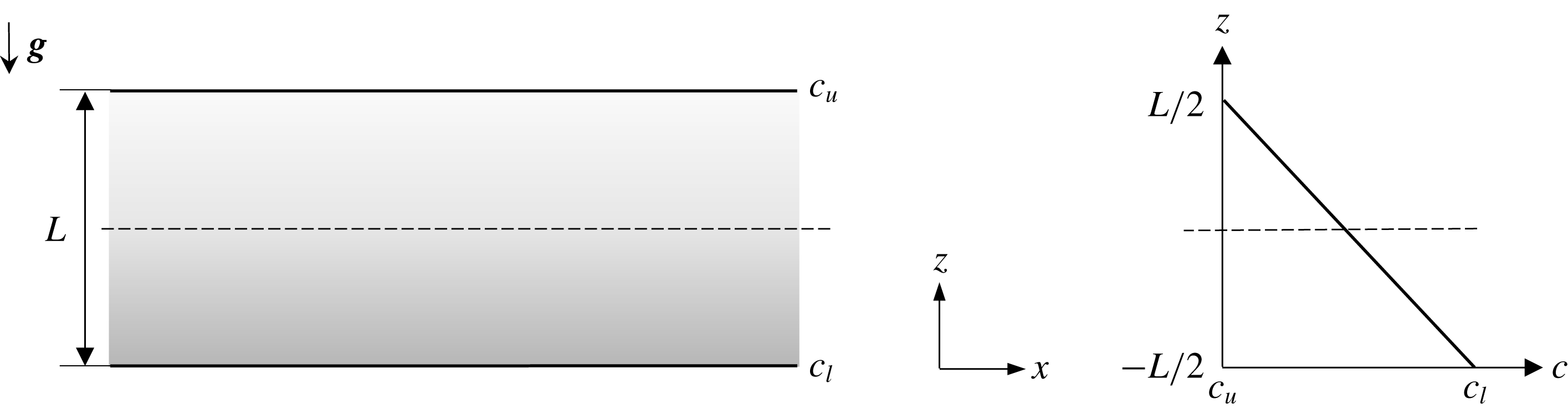
As shown in figure 1, we consider an infinite horizontal layer of near-critical binary fluid mixture of species
 $A$
and
 $B$
with a height
 $L$
under gravity. Denoting the concentration (mass fraction) of species
 $A$
as
 $c$
, the mixture considered in this study satisfies
 $(\unicode[STIX]{x2202}\unicode[STIX]{x1D70C}/\unicode[STIX]{x2202}c)_{p,T}<0$
, with
 $\unicode[STIX]{x1D70C}$
the density of the mixture,
 $T$
the temperature and
 $p$
the pressure. The horizontal and vertical directions are denoted by
 $x$
and
 $z$
, respectively. The fluid is initially motionless, homogeneous, stratified around critical density
 $\unicode[STIX]{x1D70C}_{c}$
and in thermodynamic equilibrium (
 $T=T_{r}$
, with
 $T_{r}$
the reference temperature) such that
 $$\begin{eqnarray}{\displaystyle \frac{T_{r}-T_{c}}{T_{c}}}=\unicode[STIX]{x1D700}\ll 1,\end{eqnarray}$$
where
 $T_{c}$
is the critical temperature of the binary mixture; the reduced temperature
 $\unicode[STIX]{x1D700}$
defines the dimensionless proximity to the critical point. The initial density
 $\bar{\unicode[STIX]{x1D70C}}$
and reference pressure
 $p_{ref}$
satisfy the condition of static equilibrium with the constraint of a mean density equal to
 $\unicode[STIX]{x1D70C}_{c}$
, namely
 $$\begin{eqnarray}\displaystyle \int \bar{\unicode[STIX]{x1D70C}}\,\text{d}V=\unicode[STIX]{x1D70C}_{c}V,\quad -{\displaystyle \frac{\text{d}p_{ref}}{\text{d}z}}=\bar{\unicode[STIX]{x1D70C}}g,\end{eqnarray}$$
where
 $V$
is the total volume of the physical domain. The concentration does not vary horizontally and its vertical gradient is negative (an unstable distribution);
 $c_{l}$
and
 $c_{u}$
are the concentration at the lower and upper boundaries, respectively. The lower and upper boundaries can be either rigid (no-slip) or stress-free. Mathematically, the boundary conditions are given by
 $$\begin{eqnarray}z=0:\quad \unicode[STIX]{x1D6E4}_{1}{\displaystyle \frac{\unicode[STIX]{x2202}u}{\unicode[STIX]{x2202}z}}+(1-\unicode[STIX]{x1D6E4}_{1})u=0,\quad w=0,\quad c=c_{l},\end{eqnarray}$$
 $$\begin{eqnarray}z=L:\quad \unicode[STIX]{x1D6E4}_{2}{\displaystyle \frac{\unicode[STIX]{x2202}u}{\unicode[STIX]{x2202}z}}+(1-\unicode[STIX]{x1D6E4}_{2})u=0,\quad w=0,\quad c=c_{u},\end{eqnarray}$$
where
 $u$
and
 $w$
are the horizontal and vertical components of velocity, respectively. The parameters
 $\unicode[STIX]{x1D6E4}_{1}$
and
 $\unicode[STIX]{x1D6E4}_{2}$
are set equal either to 0 for rigid boundary conditions or to 1 for stress-free ones.
Physical model for linear stability analysis. The concentration field is roughly represented as a linear function of
 $z$
.

The governing equations for binary fluid mixtures developed by Landau & Lifshitz (Reference Landau and Lifshitz1987) together with a linearized equation of state (EOS) are adopted and modified to describe a Newtonian, compressible, viscous and heat-conducting near-critical binary fluid mixture. Besides, we also treat all thermodynamic and transport properties as constant, leading to the following governing equations:
 $$\begin{eqnarray}\displaystyle & \displaystyle {\displaystyle \frac{\unicode[STIX]{x2202}\unicode[STIX]{x1D70C}}{\unicode[STIX]{x2202}t}}+\unicode[STIX]{x1D735}\boldsymbol{\cdot }(\unicode[STIX]{x1D70C}\boldsymbol{u})=0, & \displaystyle\end{eqnarray}$$
 $$\begin{eqnarray}\displaystyle & \displaystyle \unicode[STIX]{x1D70C}\left[{\displaystyle \frac{\unicode[STIX]{x2202}\boldsymbol{u}}{\unicode[STIX]{x2202}t}}+(\boldsymbol{u}\boldsymbol{\cdot }\unicode[STIX]{x1D735})\boldsymbol{u}\right]=-\unicode[STIX]{x1D735}p+\unicode[STIX]{x1D702}\unicode[STIX]{x1D6FB}^{2}\boldsymbol{u}+{\displaystyle \frac{1}{3}}\unicode[STIX]{x1D702}\unicode[STIX]{x1D735}(\unicode[STIX]{x1D735}\boldsymbol{\cdot }\boldsymbol{u})+(\unicode[STIX]{x1D70C}-\bar{\unicode[STIX]{x1D70C}})\boldsymbol{g}, & \displaystyle\end{eqnarray}$$
 $$\begin{eqnarray}\displaystyle & \displaystyle {\displaystyle \frac{\unicode[STIX]{x2202}T}{\unicode[STIX]{x2202}t}}+\boldsymbol{u}\boldsymbol{\cdot }\unicode[STIX]{x1D735}T+\unicode[STIX]{x1D735}_{ad}{\displaystyle \frac{\bar{\unicode[STIX]{x1D70C}}}{\unicode[STIX]{x1D70C}}}w={\displaystyle \frac{\unicode[STIX]{x1D706}}{\unicode[STIX]{x1D70C}c_{p}}}\unicode[STIX]{x1D6FB}^{2}T+{\displaystyle \frac{\unicode[STIX]{x1D735}_{ad}}{\unicode[STIX]{x1D70C}g}}{\displaystyle \frac{\text{D}p}{\text{D}t}}+{\displaystyle \frac{\unicode[STIX]{x1D6F7}}{\unicode[STIX]{x1D70C}c_{p}}}, & \displaystyle\end{eqnarray}$$
 $$\begin{eqnarray}\displaystyle & \displaystyle {\displaystyle \frac{\unicode[STIX]{x2202}c}{\unicode[STIX]{x2202}t}}+\boldsymbol{u}\boldsymbol{\cdot }\unicode[STIX]{x1D735}c={\displaystyle \frac{D}{\unicode[STIX]{x1D70C}}}\unicode[STIX]{x1D735}\boldsymbol{\cdot }(\unicode[STIX]{x1D70C}\unicode[STIX]{x1D735}c), & \displaystyle\end{eqnarray}$$
 $$\begin{eqnarray}\displaystyle & \displaystyle \unicode[STIX]{x1D70C}=\bar{\unicode[STIX]{x1D70C}}+\unicode[STIX]{x1D70C}_{c}[\unicode[STIX]{x1D6FC}p-\unicode[STIX]{x1D6FD}(T-\bar{T})-\unicode[STIX]{x1D705}(c-\bar{c})]. & \displaystyle\end{eqnarray}$$
Here
 $t$
is the time;
 $\boldsymbol{u}(u,w)$
is the velocity in vector form;
 $\unicode[STIX]{x1D702}$
and
 $\boldsymbol{g}(0,-g)$
are, respectively, the dynamic viscosity and the gravitational acceleration vector (
 $g=9.81~\text{m}~\text{s}^{-2}$
);
 $D$
is the diffusion coefficient;
 $c_{p}$
and
 $\unicode[STIX]{x1D706}$
are the specific heat at constant pressure and the thermal conductivity, respectively;
 $\unicode[STIX]{x1D6F7}=\unicode[STIX]{x1D702}(\unicode[STIX]{x1D735}\boldsymbol{u}+(\unicode[STIX]{x1D735}\boldsymbol{u})^{\text{T}})\boldsymbol{ : }\unicode[STIX]{x1D735}\boldsymbol{u}-(2/3)\unicode[STIX]{x1D702}(\unicode[STIX]{x1D735}\boldsymbol{\cdot }\boldsymbol{u})^{2}$
is the viscous dissipation function;
 $\unicode[STIX]{x1D6FC}=\unicode[STIX]{x1D70C}_{c}^{-1}(\unicode[STIX]{x2202}\unicode[STIX]{x1D70C}/\unicode[STIX]{x2202}p)_{T,c}$
is the isothermal compressibility;
 $\unicode[STIX]{x1D6FD}=-\unicode[STIX]{x1D70C}_{c}^{-1}(\unicode[STIX]{x2202}\unicode[STIX]{x1D70C}/\unicode[STIX]{x2202}T)_{p,c}$
is the isobaric thermal expansion coefficient;
 $\unicode[STIX]{x1D705}=-\unicode[STIX]{x1D70C}_{c}^{-1}(\unicode[STIX]{x2202}\unicode[STIX]{x1D70C}/\unicode[STIX]{x2202}c)_{p,T}$
is the concentration expansion coefficient; and
 $\unicode[STIX]{x1D735}_{ad}=-(Tg/(\unicode[STIX]{x1D70C}c_{p}))(\unicode[STIX]{x2202}\unicode[STIX]{x1D70C}/\unicode[STIX]{x2202}T)_{p,c}\approx T_{r}\unicode[STIX]{x1D6FD}g/c_{p}$
is the adiabatic temperature gradient. In addition, in the derivation of (2.6) and (2.7), a decomposition of total pressure
 $p_{total}=p_{ref}+p$
, along with (2.2), is employed.
In the present study, the role of concentration in the onset of buoyant convection in near-critical fluids is considered. To this end, we neglect cross-diffusion effects, i.e. Soret and Dufour effects, leading to the fact that mass and heat fluxes are functions of only concentration and temperature gradients, respectively. However, as pointed out by Luettmer-Strathmann (Reference Luettmer-Strathmann2002), the thermal diffusion ratio, reflecting the strength of Soret and Dufour effects, diverges close to the critical point. Therefore, the whole picture should be more complicated than that depicted in this paper. The current work paves the way for further studies.
The
 $\text{C}_{2}\text{H}_{6}$
–
 $\text{CO}_{2}$
mixture is chosen as a reference fluid system, with
 $\text{C}_{2}\text{H}_{6}$
the species
 $A$
and
 $\text{CO}_{2}$
the species
 $B$
. The average concentration of
 $\text{C}_{2}\text{H}_{6}$
is 0.005. The locus of critical points of the mixture as a function of concentration is the simplest case, connecting the critical parameters of the two components, and the experimental data on critical parameters can be found in the literature (Sengers & Jin Reference Sengers and Jin2007). Such a fluid mixture is chosen to facilitate access to critical parameters and the modelling by a cubic EOS. The physical properties of each pure compound are given in table 1.
The critical temperature
 $T_{c}$
, critical density
 $\unicode[STIX]{x1D70C}_{c}$
, critical pressure
 $p_{c}$
, molar mass
 $M$
and acentric factor
 $\unicode[STIX]{x1D714}$
of pure components. The minority species
 $\text{C}_{2}\text{H}_{6}$
is referred to as species
 $A$
, and the majority species
 $\text{CO}_{2}$
is referred to as species
 $B$
.

2.2 Modelling of physical properties
The Peng–Robinson EOS (Peng & Robinson Reference Peng and Robinson1976) along with the classical van der Waals mixing rule is chosen in this study to determine the thermodynamic properties in governing equations:
 $$\begin{eqnarray}\displaystyle & \displaystyle p={\displaystyle \frac{\unicode[STIX]{x1D70C}rT}{1-b\unicode[STIX]{x1D70C}}}-{\displaystyle \frac{a\unicode[STIX]{x1D70C}^{2}}{1+2b\unicode[STIX]{x1D70C}-(b\unicode[STIX]{x1D70C})^{2}}}, & \displaystyle\end{eqnarray}$$
 $$\begin{eqnarray}\displaystyle & \displaystyle a=\unicode[STIX]{x1D711}_{A}^{2}a_{A}+\unicode[STIX]{x1D711}_{B}^{2}a_{B}+2\unicode[STIX]{x1D711}_{A}\unicode[STIX]{x1D711}_{B}\sqrt{a_{A}a_{B}}(1-k_{AB}), & \displaystyle\end{eqnarray}$$
 $$\begin{eqnarray}\displaystyle & \displaystyle b=\unicode[STIX]{x1D711}_{A}b_{A}+\unicode[STIX]{x1D711}_{B}b_{B}, & \displaystyle\end{eqnarray}$$
where the parameter
 $r$
is calculated by
 $r=R_{g}/M$
(
 $R_{g}=8.314~\text{J}~\text{mol}^{-1}~\text{K}^{-1}$
is the universal gas constant and
 $M$
is the molar mass of the mixture);
 $\unicode[STIX]{x1D711}$
is the mole fraction; subscripts
 $A$
and
 $B$
denote the two species;
 $k_{AB}$
is the binary interaction parameter (
 $k_{AB}=0.1322$
for the
 $\text{C}_{2}\text{H}_{6}$
–
 $\text{CO}_{2}$
mixture (Fateen, Khalil & Elnabawy Reference Fateen, Khalil and Elnabawy2013)); and the parameters
 $a_{A}$
,
 $a_{B}$
,
 $b_{A}$
and
 $b_{B}$
are calculated by
 $$\begin{eqnarray}\displaystyle \left.\begin{array}{@{}c@{}}\displaystyle a_{i}=0.45723553{\displaystyle \frac{R_{g}^{2}{T_{c}}_{i}^{2}}{{p_{c}}_{i}}}\left\{1+m_{i}\left[1-\left({\displaystyle \frac{T}{{T_{c}}_{i}}}\right)^{1/2}\right]\right\}^{2},\\ \displaystyle m_{i}=0.37464+1.54226\unicode[STIX]{x1D714}_{i}-0.26992\unicode[STIX]{x1D714}_{i}^{2},\\ \displaystyle b_{i}=0.077796074{\displaystyle \frac{R_{g}{T_{c}}_{i}}{{p_{c}}_{i}}},\end{array}\right\} & & \displaystyle\end{eqnarray}$$
with the subscript
 $i=A,B$
. Calculations of
 $c_{p}$
,
 $\unicode[STIX]{x1D6FC}$
,
 $\unicode[STIX]{x1D6FD}$
and
 $\unicode[STIX]{x1D705}$
in the framework of the Peng–Robinson EOS and van der Waals mixing rule involve a lengthy computation and will not be detailed here. For a description of the procedures, the reader is referred to a detailed instruction by Pratt (Reference Pratt2001).
As for transport properties, it is supposed that the dynamic viscosity and thermal conductivity of the dilute
 $\text{C}_{2}\text{H}_{6}$
–
 $\text{CO}_{2}$
mixture are those of pure
 $\text{CO}_{2}$
under the same reduced temperature and density, which is a valid approximation for dilute mixtures (Raspo, Meradji & Zappoli Reference Raspo, Meradji and Zappoli2007). The NIST Standard Reference Database 23 (Lemmon, Huber & McLinden Reference Lemmon, Huber and McLinden2010) is used to obtain
 $\unicode[STIX]{x1D702}$
and
 $\unicode[STIX]{x1D706}$
of pure
 $\text{CO}_{2}$
. For the diffusion coefficient, since few experimental data are available, the following power law is considered (Luettmer-Strathmann Reference Luettmer-Strathmann2002):
 $$\begin{eqnarray}D=D_{0}\unicode[STIX]{x1D700}^{0.67}.\end{eqnarray}$$
The asymptotic power law introduced above is valid in a limited region around the critical point. However, as shown in Luettmer-Strathmann (Reference Luettmer-Strathmann2002), the above power law can give an approximation for
 $D$
of the
 $\text{C}_{2}\text{H}_{6}$
–
 $\text{CO}_{2}$
mixture when
 $\unicode[STIX]{x1D700}$
is less than 0.1. For
 $\unicode[STIX]{x1D700}=0.1$
, the diffusion coefficient
 $D_{\unicode[STIX]{x1D700}=0.1}$
is predicted by the model developed by Vaz et al. (Reference Vaz, Magalhães and Silva2014). Then the coefficient
 $D_{0}$
is given by
 $D_{0}=D_{\unicode[STIX]{x1D700}=0.1}/0.1^{0.67}$
.
3 Linear stability analysis
3.1 Formulation of the linear stability problem
In this section, we will follow general procedures of linear stability analysis to obtain the non-dimensional equations for the evolution of small perturbations with the help of normal-mode expansion. In fact, the physical model introduced in figure 1 can be regarded as a limiting case of double-diffusive convection (Turner Reference Turner1973), by setting the temperature gradient to zero. Similarly, the RB convection is the other limiting case of double-diffusive convection, where the influence of concentration disappears. The above facts suggest that we can directly study the general problem of double-diffusive convection. Then the limiting case studied here can be easily restored by adjusting control parameters.
For the general double-diffusive problem, the mathematical expressions for the boundary conditions should be modified to include temperature:
 $$\begin{eqnarray}z=0:\quad \unicode[STIX]{x1D6E4}_{1}{\displaystyle \frac{\unicode[STIX]{x2202}u}{\unicode[STIX]{x2202}z}}+(1-\unicode[STIX]{x1D6E4}_{1})u=0,\quad w=0,\quad T=T_{l},\quad c=c_{l},\end{eqnarray}$$
 $$\begin{eqnarray}z=L:\quad \unicode[STIX]{x1D6E4}_{2}{\displaystyle \frac{\unicode[STIX]{x2202}u}{\unicode[STIX]{x2202}z}}+(1-\unicode[STIX]{x1D6E4}_{2})u=0,\quad w=0,\quad T=T_{u},\quad c=c_{u},\end{eqnarray}$$
where
 $T_{l}$
is the temperature at the lower boundary and
 $T_{u}$
is that at the upper one. Note that
 $T_{l}=T_{u}=T_{r}$
in the original problem. The base states (denoted by the overbar symbol) of
 $u$
,
 $w$
,
 $p$
and
 $T$
are given by
 $$\begin{eqnarray}\bar{u}=\bar{w}=0,\quad \bar{p}=0,\quad \bar{T}=T_{l}-\unicode[STIX]{x1D735}_{T}z,\end{eqnarray}$$
where
 $\unicode[STIX]{x1D735}_{T}=(T_{l}-T_{u})/d$
. As for concentration and density, according to the governing equations and (2.2), their base states obey
 $$\begin{eqnarray}\displaystyle & \displaystyle \bar{\unicode[STIX]{x1D70C}}{\displaystyle \frac{\text{d}^{2}\bar{c}}{\text{d}z^{2}}}+{\displaystyle \frac{\text{d}\bar{\unicode[STIX]{x1D70C}}}{\text{d}z}}{\displaystyle \frac{\text{d}\bar{c}}{\text{d}z}}=0, & \displaystyle\end{eqnarray}$$
 $$\begin{eqnarray}\displaystyle & \displaystyle \unicode[STIX]{x1D6FC}\bar{\unicode[STIX]{x1D70C}}g+{\displaystyle \frac{1}{\unicode[STIX]{x1D70C}_{c}}}{\displaystyle \frac{\text{d}\bar{\unicode[STIX]{x1D70C}}}{\text{d}z}}=\unicode[STIX]{x1D6FD}\unicode[STIX]{x1D735}_{T}-\unicode[STIX]{x1D705}{\displaystyle \frac{\text{d}\bar{c}}{\text{d}z}}, & \displaystyle\end{eqnarray}$$
 $$\begin{eqnarray}\displaystyle & \displaystyle \displaystyle \int _{0}^{L}\bar{\unicode[STIX]{x1D70C}}\,\text{d}z=\unicode[STIX]{x1D70C}_{c}L. & \displaystyle\end{eqnarray}$$
In this study, equations (3.4) to (3.6) are solved numerically to obtain the initial fields of concentration and density. The numerical methods are elaborated in § 3.3. We now subject the base states to infinitesimal perturbations (denoted by the tilde symbol):
 $$\begin{eqnarray}u=\bar{u}+\tilde{u} ,\quad w=\bar{w}+\tilde{w},\quad T=\bar{T}+\tilde{T},\quad c=\bar{c}+\tilde{c},\quad p=\bar{p}+\tilde{p},\quad \unicode[STIX]{x1D70C}=\bar{\unicode[STIX]{x1D70C}}+\tilde{\unicode[STIX]{x1D70C}}.\quad\end{eqnarray}$$
We then substitute (3.7) into the governing equations following the standard procedures of linearization (Chandrasekhar Reference Chandrasekhar1961). Then the governing equations for small perturbations are obtained,
 $$\begin{eqnarray}\displaystyle & \displaystyle {\displaystyle \frac{\unicode[STIX]{x2202}\tilde{\unicode[STIX]{x1D70C}}}{\unicode[STIX]{x2202}t}}+\bar{\unicode[STIX]{x1D70C}}{\displaystyle \frac{\unicode[STIX]{x2202}\tilde{u} }{\unicode[STIX]{x2202}x}}+{\displaystyle \frac{\unicode[STIX]{x2202}\bar{\unicode[STIX]{x1D70C}}\tilde{w}}{\unicode[STIX]{x2202}z}}=0, & \displaystyle\end{eqnarray}$$
 $$\begin{eqnarray}\displaystyle & \displaystyle \bar{\unicode[STIX]{x1D70C}}{\displaystyle \frac{\unicode[STIX]{x2202}\tilde{u} }{\unicode[STIX]{x2202}t}}=-{\displaystyle \frac{\unicode[STIX]{x2202}\tilde{p}}{\unicode[STIX]{x2202}x}}+\unicode[STIX]{x1D702}\unicode[STIX]{x1D6FB}^{2}\tilde{u} +{\displaystyle \frac{1}{3}}\unicode[STIX]{x1D702}\left({\displaystyle \frac{\unicode[STIX]{x2202}^{2}\tilde{u} }{\unicode[STIX]{x2202}x^{2}}}+{\displaystyle \frac{\unicode[STIX]{x2202}^{2}\tilde{w}}{\unicode[STIX]{x2202}x\unicode[STIX]{x2202}z}}\right), & \displaystyle\end{eqnarray}$$
 $$\begin{eqnarray}\displaystyle & \displaystyle \bar{\unicode[STIX]{x1D70C}}{\displaystyle \frac{\unicode[STIX]{x2202}\tilde{w}}{\unicode[STIX]{x2202}t}}=-{\displaystyle \frac{\unicode[STIX]{x2202}\tilde{p}}{\unicode[STIX]{x2202}z}}+\unicode[STIX]{x1D702}\unicode[STIX]{x1D6FB}^{2}\tilde{w}+{\displaystyle \frac{1}{3}}\unicode[STIX]{x1D702}\left({\displaystyle \frac{\unicode[STIX]{x2202}^{2}\tilde{u} }{\unicode[STIX]{x2202}x\unicode[STIX]{x2202}z}}+{\displaystyle \frac{\unicode[STIX]{x2202}^{2}\tilde{w}}{\unicode[STIX]{x2202}z^{2}}}\right)-\tilde{\unicode[STIX]{x1D70C}}g, & \displaystyle\end{eqnarray}$$
 $$\begin{eqnarray}\displaystyle & \displaystyle {\displaystyle \frac{\unicode[STIX]{x2202}\tilde{T}}{\unicode[STIX]{x2202}t}}-(\unicode[STIX]{x1D735}_{T}-\unicode[STIX]{x1D735}_{ad})\tilde{w}={\displaystyle \frac{\unicode[STIX]{x1D706}}{\bar{\unicode[STIX]{x1D70C}}c_{p}}}\unicode[STIX]{x1D6FB}^{2}\tilde{T}+{\displaystyle \frac{\unicode[STIX]{x1D735}_{ad}}{\bar{\unicode[STIX]{x1D70C}}g}}{\displaystyle \frac{\unicode[STIX]{x2202}\tilde{p}}{\unicode[STIX]{x2202}t}}, & \displaystyle\end{eqnarray}$$
 $$\begin{eqnarray}\displaystyle & \displaystyle {\displaystyle \frac{\unicode[STIX]{x2202}\tilde{c}}{\unicode[STIX]{x2202}t}}+{\displaystyle \frac{\unicode[STIX]{x2202}\bar{c}}{\unicode[STIX]{x2202}z}}\tilde{w}=D\unicode[STIX]{x1D6FB}^{2}\tilde{c}+{\displaystyle \frac{D}{\bar{\unicode[STIX]{x1D70C}}}}{\displaystyle \frac{\unicode[STIX]{x2202}\bar{c}}{\unicode[STIX]{x2202}z}}{\displaystyle \frac{\unicode[STIX]{x2202}\tilde{\unicode[STIX]{x1D70C}}}{\unicode[STIX]{x2202}z}}+{\displaystyle \frac{D}{\bar{\unicode[STIX]{x1D70C}}}}{\displaystyle \frac{\unicode[STIX]{x2202}\bar{\unicode[STIX]{x1D70C}}}{\unicode[STIX]{x2202}z}}{\displaystyle \frac{\unicode[STIX]{x2202}\tilde{c}}{\unicode[STIX]{x2202}z}}, & \displaystyle\end{eqnarray}$$
 $$\begin{eqnarray}\displaystyle & \displaystyle \tilde{\unicode[STIX]{x1D70C}}=\unicode[STIX]{x1D70C}_{c}(\unicode[STIX]{x1D6FC}\tilde{p}-\unicode[STIX]{x1D6FD}\tilde{T}-\unicode[STIX]{x1D705}\tilde{c}), & \displaystyle\end{eqnarray}$$
together with the boundary conditions,
 $$\begin{eqnarray}z=0\text{ and }L:\quad \unicode[STIX]{x1D6E4}_{i}{\displaystyle \frac{\unicode[STIX]{x2202}\tilde{u} }{\unicode[STIX]{x2202}z}}+(1-\unicode[STIX]{x1D6E4}_{i})\tilde{u} =0,\quad \tilde{w}=0,\quad \tilde{T}=0,\quad \tilde{c}=0,\end{eqnarray}$$
where
 $i=1$
for
 $z=0$
, and
 $i=2$
for
 $z=L$
.
The above governing equations are made non-dimensional by defining the following non-dimensional quantities (indicated by prime symbol):
 $$\begin{eqnarray}(x,z)=(x^{\prime },z^{\prime })L,\quad t=t^{\prime }{\displaystyle \frac{L^{2}}{D_{T}}},\end{eqnarray}$$
 $$\begin{eqnarray}(\tilde{u} ,\tilde{w})=(u^{\prime },w^{\prime }){\displaystyle \frac{D_{T}}{L}},\end{eqnarray}$$
 $$\begin{eqnarray}\displaystyle \tilde{T}=T^{\prime }(\unicode[STIX]{x1D735}_{T}-\unicode[STIX]{x1D735}_{ad})L,\quad \bar{c}=\bar{c}^{\prime }\unicode[STIX]{x1D735}_{c}L+c_{l},\quad \tilde{c}=c^{\prime }\unicode[STIX]{x1D735}_{c}L,\end{eqnarray}$$
 $$\begin{eqnarray}\tilde{p}=p^{\prime }{\displaystyle \frac{\unicode[STIX]{x1D702}D_{T}}{L^{2}}},\quad (\tilde{\unicode[STIX]{x1D70C}},\bar{\unicode[STIX]{x1D70C}})=(\unicode[STIX]{x1D70C}^{\prime },\bar{\unicode[STIX]{x1D70C}}^{\prime })\unicode[STIX]{x1D70C}_{c},\end{eqnarray}$$
in which
 $\unicode[STIX]{x1D735}_{c}=(c_{l}-c_{u})/d$
and
 $D_{T}=\unicode[STIX]{x1D706}/(\unicode[STIX]{x1D70C}_{c}c_{p})$
is the thermal diffusivity. The scaling factor for temperature perturbation used here is unusual – a more general one should be
 $\unicode[STIX]{x1D735}_{T}L$
. Recall that the RB problem is a limiting case of double-diffusive convection. Therefore, the scaling factor for temperature should guarantee that the modified Rayleigh number given in (1.1), instead of the normal Rayleigh number, is a control parameter in the general double-diffusive problem. After several attempts, we found choosing
 $(\unicode[STIX]{x1D735}_{T}-\unicode[STIX]{x1D735}_{ad})L$
as the scaling factor of temperature perturbation works. Physically speaking,
 $(\unicode[STIX]{x1D735}_{T}-\unicode[STIX]{x1D735}_{ad})$
is the effective temperature gradient to induce convection, in which the stabilizing effect of
 $\unicode[STIX]{x1D735}_{ad}$
is deducted. The system of equations is scaled on the typical time scale of thermal diffusivity. The non-dimensional equations for the evolution of small perturbations are
 $$\begin{eqnarray}\displaystyle & \displaystyle {\displaystyle \frac{\unicode[STIX]{x2202}\unicode[STIX]{x1D70C}^{\prime }}{\unicode[STIX]{x2202}t^{\prime }}}+\bar{\unicode[STIX]{x1D70C}}^{\prime }{\displaystyle \frac{\unicode[STIX]{x2202}u^{\prime }}{\unicode[STIX]{x2202}x^{\prime }}}+{\displaystyle \frac{\unicode[STIX]{x2202}\bar{\unicode[STIX]{x1D70C}}^{\prime }w^{\prime }}{\unicode[STIX]{x2202}z^{\prime }}}=0, & \displaystyle\end{eqnarray}$$
 $$\begin{eqnarray}\displaystyle & \displaystyle {\displaystyle \frac{\bar{\unicode[STIX]{x1D70C}}^{\prime }}{Pr}}{\displaystyle \frac{\unicode[STIX]{x2202}u^{\prime }}{\unicode[STIX]{x2202}t^{\prime }}}=-{\displaystyle \frac{\unicode[STIX]{x2202}p^{\prime }}{\unicode[STIX]{x2202}x^{\prime }}}+\unicode[STIX]{x1D6FB}^{2}u^{\prime }+{\displaystyle \frac{1}{3}}\left({\displaystyle \frac{\unicode[STIX]{x2202}^{2}u^{\prime }}{\unicode[STIX]{x2202}{x^{\prime }}^{2}}}+{\displaystyle \frac{\unicode[STIX]{x2202}^{2}w^{\prime }}{\unicode[STIX]{x2202}x^{\prime }\unicode[STIX]{x2202}z^{\prime }}}\right), & \displaystyle\end{eqnarray}$$
 $$\begin{eqnarray}\displaystyle & \displaystyle {\displaystyle \frac{\bar{\unicode[STIX]{x1D70C}}^{\prime }}{Pr}}{\displaystyle \frac{\unicode[STIX]{x2202}w^{\prime }}{\unicode[STIX]{x2202}t^{\prime }}}=-{\displaystyle \frac{\unicode[STIX]{x2202}p^{\prime }}{\unicode[STIX]{x2202}z^{\prime }}}+\unicode[STIX]{x1D6FB}^{2}w^{\prime }+{\displaystyle \frac{1}{3}}\left({\displaystyle \frac{\unicode[STIX]{x2202}^{2}u^{\prime }}{\unicode[STIX]{x2202}x^{\prime }\unicode[STIX]{x2202}z^{\prime }}}+{\displaystyle \frac{\unicode[STIX]{x2202}^{2}w^{\prime }}{\unicode[STIX]{x2202}{z^{\prime }}^{2}}}\right)-\unicode[STIX]{x1D712}p^{\prime }+RT^{\prime }+R_{c}c^{\prime }, & \displaystyle\end{eqnarray}$$
 $$\begin{eqnarray}\displaystyle & \displaystyle {\displaystyle \frac{\unicode[STIX]{x2202}T^{\prime }}{\unicode[STIX]{x2202}t^{\prime }}}-w^{\prime }={\displaystyle \frac{1}{\bar{\unicode[STIX]{x1D70C}}^{\prime }}}\left(\unicode[STIX]{x1D6FB}^{2}T^{\prime }+{\displaystyle \frac{R_{p}R_{ad}}{R}}{\displaystyle \frac{\unicode[STIX]{x2202}p^{\prime }}{\unicode[STIX]{x2202}t^{\prime }}}\right), & \displaystyle\end{eqnarray}$$
 $$\begin{eqnarray}\displaystyle & \displaystyle {\displaystyle \frac{\unicode[STIX]{x2202}c^{\prime }}{\unicode[STIX]{x2202}t^{\prime }}}+{\displaystyle \frac{\text{d}\bar{c}^{\prime }}{\text{d}z^{\prime }}}w^{\prime }=\unicode[STIX]{x1D70F}\unicode[STIX]{x1D6FB}^{2}c^{\prime }+{\displaystyle \frac{\unicode[STIX]{x1D70F}}{\bar{\unicode[STIX]{x1D70C}}^{\prime }}}\left({\displaystyle \frac{\text{d}\bar{c}^{\prime }}{\text{d}z^{\prime }}}{\displaystyle \frac{\unicode[STIX]{x2202}\unicode[STIX]{x1D70C}^{\prime }}{\unicode[STIX]{x2202}z^{\prime }}}+{\displaystyle \frac{\text{d}\bar{\unicode[STIX]{x1D70C}}^{\prime }}{\text{d}z^{\prime }}}{\displaystyle \frac{\unicode[STIX]{x2202}c^{\prime }}{\unicode[STIX]{x2202}z^{\prime }}}\right), & \displaystyle\end{eqnarray}$$
 $$\begin{eqnarray}\displaystyle & \displaystyle \unicode[STIX]{x1D70C}^{\prime }=R_{p}(\unicode[STIX]{x1D712}p^{\prime }-RT^{\prime }-R_{c}c^{\prime }). & \displaystyle\end{eqnarray}$$
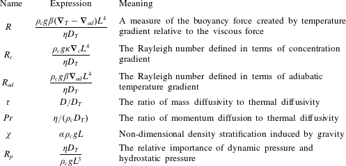
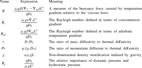
The expressions for and physical meanings of the non-dimensional numbers in the above equations are summarized in table 2.
We now make a normal-mode expansion by letting
 $$\begin{eqnarray}[u^{\prime },w^{\prime },p^{\prime },T^{\prime },c^{\prime },\unicode[STIX]{x1D70C}^{\prime }]=[\hat{u} (z^{\prime }),{\hat{w}}(z^{\prime }),\hat{p}(z^{\prime }),\hat{T}(z^{\prime }),{\hat{c}}(z^{\prime }),\hat{\unicode[STIX]{x1D70C}}(z^{\prime })]\exp (\text{i}kx^{\prime }+\unicode[STIX]{x1D70E}t^{\prime }).\end{eqnarray}$$
Here
 $\unicode[STIX]{x1D70E}$
is the growth rate and
 $k$
is the horizontal wavenumber, both of which are non-dimensional. (3.19)–(3.24) then give
 $$\begin{eqnarray}\displaystyle & & \displaystyle \left({\mathcal{D}}^{2}-{\displaystyle \frac{4}{3}}k^{2}\right)\hat{u} +{\displaystyle \frac{1}{3}}\text{i}k{\mathcal{D}}{\hat{w}}-\text{i}k\hat{p}=\unicode[STIX]{x1D70E}\left({\displaystyle \frac{1}{Pr}}\bar{\unicode[STIX]{x1D70C}}^{\prime }\hat{u} \right),\end{eqnarray}$$
 $$\begin{eqnarray}\displaystyle & & \displaystyle {\displaystyle \frac{1}{3}}\text{i}k{\mathcal{D}}\hat{u} +\left({\displaystyle \frac{4}{3}}{\mathcal{D}}^{2}-k^{2}\right){\hat{w}}+R\hat{T}+R_{c}{\hat{c}}-({\mathcal{D}}+\unicode[STIX]{x1D712})\hat{p}=\unicode[STIX]{x1D70E}\left({\displaystyle \frac{1}{Pr}}\bar{\unicode[STIX]{x1D70C}}^{\prime }{\hat{w}}\right),\end{eqnarray}$$
 $$\begin{eqnarray}\displaystyle & & \displaystyle {\hat{w}}+{\displaystyle \frac{1}{\bar{\unicode[STIX]{x1D70C}}^{\prime }}}({\mathcal{D}}^{2}-k^{2})\hat{T}=\unicode[STIX]{x1D70E}\left(\hat{T}-{\displaystyle \frac{1}{\bar{\unicode[STIX]{x1D70C}}^{\prime }}}{\displaystyle \frac{R_{p}R_{ad}}{R}}\hat{p}\right),\end{eqnarray}$$
 $$\begin{eqnarray}\displaystyle & & \displaystyle -\bar{c}_{z}{\hat{w}}+\unicode[STIX]{x1D70F}\left[{\mathcal{D}}^{2}-k^{2}+{\displaystyle \frac{1}{\bar{\unicode[STIX]{x1D70C}}^{\prime }}}(\bar{\unicode[STIX]{x1D70C}}_{z}-R_{p}R_{c}\bar{c}_{z}){\mathcal{D}}\right]{\hat{c}}\nonumber\\ \displaystyle & & \displaystyle \quad +\,{\displaystyle \frac{\unicode[STIX]{x1D70F}R_{p}\bar{c}_{z}}{\bar{\unicode[STIX]{x1D70C}}^{\prime }}}(\unicode[STIX]{x1D712}{\mathcal{D}}\hat{p}-R{\mathcal{D}}\hat{T})=\unicode[STIX]{x1D70E}{\hat{c}},\end{eqnarray}$$
 $$\begin{eqnarray}\displaystyle & & \displaystyle -\text{i}k\bar{\unicode[STIX]{x1D70C}}^{\prime }\hat{u} -(\bar{\unicode[STIX]{x1D70C}}_{z}+\bar{\unicode[STIX]{x1D70C}}^{\prime }{\mathcal{D}}){\hat{w}}=\unicode[STIX]{x1D70E}[R_{p}(\unicode[STIX]{x1D712}\hat{p}-R\hat{T}-R_{c}{\hat{c}})],\end{eqnarray}$$
where
 ${\mathcal{D}}=\text{d}/\text{d}z^{\prime }$
, and
 $\bar{c}_{z}=\text{d}\bar{c}^{\prime }/\text{d}z^{\prime }$
and
 $\bar{\unicode[STIX]{x1D70C}}_{z}=\text{d}\bar{\unicode[STIX]{x1D70C}}^{\prime }/\text{d}z^{\prime }$
, respectively, are non-dimensional concentration and density gradients along the
 $z$
direction. Owing to its complexity, the above system of equations is solved numerically to obtain the perturbation profiles and
 $\unicode[STIX]{x1D70E}$
for a given
 $k$
. The numerical method will be detailed in § 3.3. Before that, let us first consider a limiting case under the Boussinesq approximation, which has been widely used in common fluids for RB and double-diffusive instabilities. It brings huge simplifications to the governing equations, making it possible to obtain an analytical criterion for the onset of convection (Turner Reference Turner1973). In the next section, we will apply the Boussinesq approximation to the original governing equations and obtain the equations for small perturbations. The previous theoretical criterion is then briefly reviewed.
3.2 A limiting case: Boussinesq approximation
In the Boussinesq approximation, density variations are ignored except for the buoyancy term in the momentum equation, which brings significant simplifications and makes the mathematics and physics simpler. Applying the Boussinesq approximation, the aforementioned procedures give the following governing equations for small perturbations:
 $$\begin{eqnarray}\displaystyle & \displaystyle {\displaystyle \frac{\unicode[STIX]{x2202}\unicode[STIX]{x1D6FB}^{2}\tilde{w}}{\unicode[STIX]{x2202}t}}={\displaystyle \frac{\unicode[STIX]{x1D702}}{\unicode[STIX]{x1D70C}_{c}}}\unicode[STIX]{x1D6FB}^{4}\tilde{w}+\unicode[STIX]{x1D6FD}g{\displaystyle \frac{\unicode[STIX]{x2202}^{2}\tilde{T}}{\unicode[STIX]{x2202}x^{2}}}+\unicode[STIX]{x1D705}g{\displaystyle \frac{\unicode[STIX]{x2202}^{2}\tilde{c}}{\unicode[STIX]{x2202}x^{2}}}, & \displaystyle\end{eqnarray}$$
 $$\begin{eqnarray}\displaystyle & \displaystyle {\displaystyle \frac{\unicode[STIX]{x2202}\tilde{T}}{\unicode[STIX]{x2202}t}}-(\unicode[STIX]{x1D735}_{T}-\unicode[STIX]{x1D735}_{ad})\tilde{w}=D_{T}\unicode[STIX]{x1D6FB}^{2}\tilde{T}, & \displaystyle\end{eqnarray}$$
 $$\begin{eqnarray}\displaystyle & \displaystyle {\displaystyle \frac{\unicode[STIX]{x2202}\tilde{c}}{\unicode[STIX]{x2202}t}}-\unicode[STIX]{x1D735}_{c}\tilde{w}=D\unicode[STIX]{x1D6FB}^{2}\tilde{c}, & \displaystyle\end{eqnarray}$$
in which the incompressible continuity equation and two momentum equations have been combined and simplified into one single equation in
 $w$
. The boundary conditions are
 $$\begin{eqnarray}z=0\text{ and }L:\quad \unicode[STIX]{x1D6E4}_{i}{\displaystyle \frac{\unicode[STIX]{x2202}^{2}\tilde{w}}{\unicode[STIX]{x2202}z^{2}}}+(1-\unicode[STIX]{x1D6E4}_{i}){\displaystyle \frac{\unicode[STIX]{x2202}\tilde{w}}{\unicode[STIX]{x2202}z}}=0,\quad \tilde{w}=0,\quad \tilde{T}=0,\quad \tilde{c}=0,\end{eqnarray}$$
where
 $i=1$
for
 $z=0$
, and
 $i=2$
for
 $z=L$
. It should be noted that such a set of equations is widely used to describe double-diffusive convection in geophysics or astrophysics, where the adiabatic temperature gradient plays an important role for weakly compressible fluids in large spatial scales (Garaud Reference Garaud2018). However, the role of adiabatic temperature gradient becomes important in the critical region even in small spatial scales due to the strong compressibility. This is an important character of near-critical fluids and has been reported before in studies about RB instability for near-critical pure fluids (Carlès & Ugurtas Reference Carlès and Ugurtas1999). Now we have three equations for
 $\tilde{w}$
,
 $\tilde{T}$
and
 $\tilde{c}$
. Substituting the non-dimensional variables defined earlier gives
 $$\begin{eqnarray}\displaystyle & \displaystyle {\displaystyle \frac{1}{Pr}}{\displaystyle \frac{\unicode[STIX]{x2202}\unicode[STIX]{x1D6FB}^{2}w^{\prime }}{\unicode[STIX]{x2202}t^{\prime }}}=\unicode[STIX]{x1D6FB}^{4}w^{\prime }+R{\displaystyle \frac{\unicode[STIX]{x2202}^{2}T^{\prime }}{\unicode[STIX]{x2202}{x^{\prime }}^{2}}}+R_{c}{\displaystyle \frac{\unicode[STIX]{x2202}^{2}c^{\prime }}{\unicode[STIX]{x2202}{x^{\prime }}^{2}}}, & \displaystyle\end{eqnarray}$$
 $$\begin{eqnarray}\displaystyle & \displaystyle {\displaystyle \frac{\unicode[STIX]{x2202}T^{\prime }}{\unicode[STIX]{x2202}t^{\prime }}}-w^{\prime }=\unicode[STIX]{x1D6FB}^{2}T^{\prime }, & \displaystyle\end{eqnarray}$$
 $$\begin{eqnarray}\displaystyle & \displaystyle {\displaystyle \frac{\unicode[STIX]{x2202}c^{\prime }}{\unicode[STIX]{x2202}t^{\prime }}}-w^{\prime }=\unicode[STIX]{x1D70F}\unicode[STIX]{x1D6FB}^{2}c^{\prime }, & \displaystyle\end{eqnarray}$$
in which the definitions of non-dimensional numbers are the same as introduced before (see table 2). Finally, we make a normal-mode expansion by letting
 $$\begin{eqnarray}[w^{\prime },T^{\prime },c^{\prime }]=[{\hat{w}}(z^{\prime }),\hat{T}(z^{\prime }),{\hat{c}}(z^{\prime })]\exp (\text{i}kx^{\prime }+\unicode[STIX]{x1D70E}t^{\prime }).\end{eqnarray}$$
Then the counterparts of (3.26)–(3.30) under the Boussinesq approximation are given by
 $$\begin{eqnarray}\displaystyle & \displaystyle ({\mathcal{D}}^{4}-2k^{2}{\mathcal{D}}^{2}+k^{4}){\hat{w}}-k^{2}R\hat{T}-k^{2}R_{c}{\hat{c}}=\unicode[STIX]{x1D70E}{\displaystyle \frac{({\mathcal{D}}^{2}-k^{2})}{Pr}}{\hat{w}}, & \displaystyle\end{eqnarray}$$
 $$\begin{eqnarray}\displaystyle & \displaystyle {\hat{w}}+({\mathcal{D}}^{2}-k^{2})\hat{T}=\unicode[STIX]{x1D70E}\hat{T}, & \displaystyle\end{eqnarray}$$
 $$\begin{eqnarray}\displaystyle & \displaystyle {\hat{w}}+\unicode[STIX]{x1D70F}({\mathcal{D}}^{2}-k^{2}){\hat{c}}=\unicode[STIX]{x1D70E}{\hat{c}}. & \displaystyle\end{eqnarray}$$
It is clearly shown that the Boussinesq approximation brings huge simplifications to the final equations after normal-mode expansion, which allows for the analytical solution of the neutral curve. According to Baines & Gill (Reference Baines and Gill1969), when
 $R_{c}>0$
, as is currently the case, the neutral stability curve is given by
 $$\begin{eqnarray}R+{\displaystyle \frac{R_{c}}{\unicode[STIX]{x1D70F}}}=R^{cri},\end{eqnarray}$$
where
 $R^{cri}$
is the same critical Rayleigh number as in the RB problem, which has been discussed in § 1.
In a later section, we will compare the neutral stability parameters obtained from the full equations and those from the Boussinesq equations, and then the applicability of the Boussinesq approximation is discussed based on the comparisons. If the predicted parameters are almost the same, it suggests that the effects neglected in the Boussinesq approximation are insignificant and the approximation is applicable. As a result, the criterion for convection onset is naturally obtained.
3.3 Numerical method
The physical space
 $z^{\prime }=[0,1]$
is uniformly divided into
 $N$
grid points, in which the first and the last grid points are on the bottom and top boundaries, respectively. A finite difference technique is used to discretize the equations. The spatial derivatives are discretized with second-order central difference schemes such that
 $$\begin{eqnarray}\displaystyle & \displaystyle {\mathcal{D}}\unicode[STIX]{x1D719}_{j}={\displaystyle \frac{\text{d}\unicode[STIX]{x1D719}_{j}}{\text{d}z^{\prime }}}={\displaystyle \frac{\unicode[STIX]{x1D719}_{j+1}-\unicode[STIX]{x1D719}_{j-1}}{2\unicode[STIX]{x1D6FF}z}}, & \displaystyle\end{eqnarray}$$
 $$\begin{eqnarray}\displaystyle & \displaystyle {\mathcal{D}}^{2}\unicode[STIX]{x1D719}_{j}={\displaystyle \frac{\text{d}^{2}\unicode[STIX]{x1D719}_{j}}{\text{d}{z^{\prime }}^{2}}}={\displaystyle \frac{\unicode[STIX]{x1D719}_{j+1}-2\unicode[STIX]{x1D719}_{j}+\unicode[STIX]{x1D719}_{j-1}}{\unicode[STIX]{x1D6FF}z^{2}}}, & \displaystyle\end{eqnarray}$$
 $$\begin{eqnarray}\displaystyle & \displaystyle {\mathcal{D}}^{4}\unicode[STIX]{x1D719}_{j}={\displaystyle \frac{\text{d}^{4}\unicode[STIX]{x1D719}_{j}}{\text{d}{z^{\prime }}^{4}}}={\displaystyle \frac{\unicode[STIX]{x1D719}_{j+2}-4\unicode[STIX]{x1D719}_{j+1}+6\unicode[STIX]{x1D719}_{j}-4\unicode[STIX]{x1D719}_{j-1}+\unicode[STIX]{x1D719}_{j-2}}{\unicode[STIX]{x1D6FF}z^{4}}}, & \displaystyle\end{eqnarray}$$
for
 $j=2,3,\ldots ,N-1$
, where
 $\unicode[STIX]{x1D6FF}z=1/(N-1)$
is the non-dimensional distance between two adjacent grid points,
 $\unicode[STIX]{x1D719}$
represents a physical variable defined on the domain, and subscript
 $j$
is the index of a grid point.
Let us first consider the base states of concentration
 $\bar{c}^{\prime }$
and density
 $\bar{\unicode[STIX]{x1D70C}}^{\prime }$
. We construct iteration formulas as follows:
 $$\begin{eqnarray}\displaystyle & \displaystyle \bar{\unicode[STIX]{x1D70C}}^{\prime \,n+1}=C\exp \left(\displaystyle \int _{0}^{z^{\prime }}\unicode[STIX]{x1D711}^{n}\,\text{d}z^{\prime }\right), & \displaystyle\end{eqnarray}$$
 $$\begin{eqnarray}\displaystyle & \displaystyle \bar{\unicode[STIX]{x1D70C}}^{\prime \,n+1}{\displaystyle \frac{\text{d}^{2}\bar{c}^{\prime \,n+1}}{\text{d}{z^{\prime }}^{\,2}}}+{\displaystyle \frac{\text{d}\bar{\unicode[STIX]{x1D70C}}^{\prime \,n+1}}{\text{d}z^{\prime }}}{\displaystyle \frac{\text{d}\bar{c}^{\prime \,n+1}}{\text{d}z^{\prime }}}=0, & \displaystyle\end{eqnarray}$$
where
 $$\begin{eqnarray}\displaystyle & \displaystyle \unicode[STIX]{x1D711}^{n}={\displaystyle \frac{R_{p}}{\bar{\unicode[STIX]{x1D70C}}^{\prime \,n}}}\left(R+R_{ad}-R_{c}{\displaystyle \frac{\text{d}\bar{c}^{\prime \,n}}{\text{d}z^{\prime }}}\right)-\unicode[STIX]{x1D712}, & \displaystyle\end{eqnarray}$$
 $$\begin{eqnarray}\displaystyle & \displaystyle C={\displaystyle \frac{1}{\displaystyle \int _{0}^{1}\exp \left(\displaystyle \int _{0}^{z^{\prime }}\unicode[STIX]{x1D711}^{n}\,\text{d}z^{\prime }\right)\,\text{d}z^{\prime }}}, & \displaystyle\end{eqnarray}$$
and the superscript
 $n$
indicates the number of iterations. Then (3.46) and (3.47) are discretized based on the schemes given by (3.43) and (3.44). The former is transformed into an explicit system of equations, whose solution is determined directly. However, the latter results in an implicit tridiagonal system of equations, which is solved by a tridiagonal matrix algorithm (Thomas Reference Thomas1949). The discretized equations are solved iteratively, until the following convergence criterion is reached:
 $$\begin{eqnarray}{\displaystyle \frac{\mathop{\sum }_{i=1}^{N}|\unicode[STIX]{x1D719}_{i}^{k+1}-\unicode[STIX]{x1D719}_{i}^{k}|}{\mathop{\sum }_{i=1}^{N}\unicode[STIX]{x1D719}_{i}^{k}}}\leqslant 10^{-6}.\end{eqnarray}$$
Now we discuss the method for solving the equations after normal-mode expansion. Using the aforementioned difference schemes for space derivatives, the two sets of normal-mode equations, (3.26)–(3.30) and (3.39)–(3.41), are discretized and yield
 $$\begin{eqnarray}\unicode[STIX]{x1D63C}\unicode[STIX]{x1D641}=\unicode[STIX]{x1D70E}\unicode[STIX]{x1D63D}\unicode[STIX]{x1D641},\end{eqnarray}$$
with
 $$\begin{eqnarray}\unicode[STIX]{x1D63C}=\left[\begin{array}{@{}ccccc@{}}\unicode[STIX]{x1D63C}_{u1} & {\unicode[STIX]{x1D63C}_{w}}_{1} & 0 & 0 & \unicode[STIX]{x1D63C}_{p1}\\ \unicode[STIX]{x1D63C}_{u2} & \unicode[STIX]{x1D63C}_{w2} & \unicode[STIX]{x1D63C}_{T2} & \unicode[STIX]{x1D63C}_{c2} & \unicode[STIX]{x1D63C}_{p2}\\ 0 & \unicode[STIX]{x1D63C}_{w3} & \unicode[STIX]{x1D63C}_{T3} & 0 & 0\\ 0 & \unicode[STIX]{x1D63C}_{w4} & \unicode[STIX]{x1D63C}_{T4} & \unicode[STIX]{x1D63C}_{c4} & \unicode[STIX]{x1D63C}_{p4}\\ \unicode[STIX]{x1D63C}_{u5} & \unicode[STIX]{x1D63C}_{w5} & 0 & 0 & 0\end{array}\right],\quad \unicode[STIX]{x1D641}=\left[\begin{array}{@{}c@{}}\hat{\unicode[STIX]{x1D66A}}\\ \hat{\unicode[STIX]{x1D66C}}\\ \hat{\unicode[STIX]{x1D64F}}\\ \hat{\unicode[STIX]{x1D658}}\\ \hat{\unicode[STIX]{x1D665}}\end{array}\right],\quad \unicode[STIX]{x1D63D}=\left[\begin{array}{@{}ccccc@{}}\unicode[STIX]{x1D63D}_{u1} & 0 & 0 & 0 & 0\\ 0 & \unicode[STIX]{x1D63D}_{w2} & 0 & 0 & 0\\ 0 & 0 & \unicode[STIX]{x1D63D}_{T3} & 0 & \unicode[STIX]{x1D63D}_{p3}\\ 0 & 0 & 0 & \unicode[STIX]{x1D63D}_{c4} & 0\\ 0 & 0 & \unicode[STIX]{x1D63D}_{T5} & \unicode[STIX]{x1D63D}_{c5} & \unicode[STIX]{x1D63D}_{p5}\end{array}\right],\end{eqnarray}$$
for full equations, and
 $$\begin{eqnarray}\unicode[STIX]{x1D63C}=\left[\begin{array}{@{}ccc@{}}{\unicode[STIX]{x1D63C}_{w}}_{1} & \unicode[STIX]{x1D63C}_{T1} & \unicode[STIX]{x1D63C}_{c1}\\ {\unicode[STIX]{x1D63C}_{w}}_{2} & \unicode[STIX]{x1D63C}_{T2} & 0\\ {\unicode[STIX]{x1D63C}_{w}}_{3} & 0 & \unicode[STIX]{x1D63C}_{c3}\end{array}\right],\quad \unicode[STIX]{x1D63D}=\left[\begin{array}{@{}ccc@{}}{\unicode[STIX]{x1D63D}_{w}}_{1} & 0 & 0\\ 0 & \unicode[STIX]{x1D63D}_{T2} & 0\\ 0 & 0 & \unicode[STIX]{x1D63D}_{c3}\end{array}\right],\quad \unicode[STIX]{x1D641}=\left[\begin{array}{@{}c@{}}\hat{\unicode[STIX]{x1D66C}}\\ \hat{\unicode[STIX]{x1D64F}}\\ \hat{\unicode[STIX]{x1D658}}\end{array}\right],\end{eqnarray}$$
for Boussinesq equations. Matrices
 $\unicode[STIX]{x1D63C}_{u1}$
,
 $\unicode[STIX]{x1D63C}_{w1},\ldots$
and
 $\unicode[STIX]{x1D63D}_{u1}$
,
 $\unicode[STIX]{x1D63D}_{w2},\ldots$
are square matrices of dimension
 $(N-2)\times (N-2)$
, where the first subscript denotes the variable from which it originates, and the second subscript indicates the number of the sequence of the equation to which it belongs. Vectors
 $\hat{\unicode[STIX]{x1D66A}}$
,
 $\hat{\unicode[STIX]{x1D66C}}$
,
 $\hat{\unicode[STIX]{x1D64F}},\ldots$
are column vectors of dimension
 $(N-2)\times 1$
, representing the discretized physical variables. From a mathematical point of view, the problem is now transformed into a generalized eigenvalue problem of square matrices
 $\unicode[STIX]{x1D63C}$
and
 $\unicode[STIX]{x1D63D}$
(Mamou, Vasseur & Hasnaoui Reference Mamou, Vasseur and Hasnaoui2001). For a given set of governing parameters,
 $R$
,
 $R_{ad}$
,
 $R_{c}$
,
 $Pr$
,
 $\unicode[STIX]{x1D70F}$
,
 $\unicode[STIX]{x1D712}$
,
 $R_{p}$
,
 $\unicode[STIX]{x1D6E4}_{1}$
,
 $\unicode[STIX]{x1D6E4}_{2}$
and
 $k$
, the eigenvalues
 $\unicode[STIX]{x1D70E}$
and eigenvectors
 $\unicode[STIX]{x1D641}$
of the above systems are obtained through the ‘eig’ function in the NumPy library for Python (Jones et al.
Reference Jones, Oliphant and Peterson2001). Then the eigenvalues are ranked in decreasing order, and we mainly focus on the first eigenvalue
 $\unicode[STIX]{x1D70E}_{1}$
and the corresponding eigenvector, since it defines the most unstable mode.
We recall that, in the original problem,
 $\unicode[STIX]{x1D735}_{T}$
is equal to zero, leading to
 $R=-R_{ad}$
(see the definition of
 $R$
in table 2). In addition, if the reduced temperature
 $\unicode[STIX]{x1D700}$
and height
 $L$
are fixed,
 $R_{ad}$
,
 $\unicode[STIX]{x1D70F}$
,
 $Pr$
,
 $\unicode[STIX]{x1D712}$
and
 $R_{p}$
are also determined. Therefore, the present problem is actually governed by six parameters:
 $R_{c}$
,
 $k$
,
 $\unicode[STIX]{x1D6E4}_{1}$
,
 $\unicode[STIX]{x1D6E4}_{2}$
,
 $\unicode[STIX]{x1D700}$
and
 $L$
. This work focuses on the criterion for convection onset. In order words, we need to find the critical concentration Rayleigh number
 $R_{c}^{cri}$
, namely the minimum
 $R_{c}$
that makes
 $\unicode[STIX]{x1D70E}_{1}=0$
for only one wavenumber and
 $\unicode[STIX]{x1D70E}_{1}<0$
for all other wavenumbers, under given
 $\unicode[STIX]{x1D6E4}_{1}$
,
 $\unicode[STIX]{x1D6E4}_{2}$
,
 $\unicode[STIX]{x1D700}$
and
 $L$
. In order to save CPU time, the golden-section search technique is employed in the algorithm. The calculations were performed for various
 $\unicode[STIX]{x1D6E4}_{1}$
,
 $\unicode[STIX]{x1D6E4}_{2}$
,
 $\unicode[STIX]{x1D700}$
and
 $L$
and for both full equations and Boussinesq equations. The results and comparisons are performed in the next section.
3.4 Results and comparisons
From a theoretical point of view, according to (3.42), when
 $\unicode[STIX]{x1D735}_{T}=0$
, namely
 $R=-R_{ad}$
, the critical concentration Rayleigh number
 $R_{c}^{cri}$
is given by
 $$\begin{eqnarray}R_{c}^{cri}=\unicode[STIX]{x1D70F}(R^{cri}+R_{ad}).\end{eqnarray}$$
First of all, in order to validate our numerical code and study the effect of grid size on numerical results, we compare in table 3 the
 $R_{c}^{cri}$
calculated from the Boussinesq equations and predicted by (3.54). It is shown that, as the grid number is increased, the calculated critical parameters converge towards the one predicted by (3.54), which proves the validity of our numerical code.
Effect of the grid number on the computed critical concentration Rayleigh number
 $R_{c,Bou}^{cri}$
for Boussinesq equations (
 $\unicode[STIX]{x1D700}=0.001$
,
 $\unicode[STIX]{x1D6E4}_{1}=0$
,
 $\unicode[STIX]{x1D6E4}_{2}=1$
and
 $L=10$
mm). Here
 $R_{c,the}^{cri}$
is the theoretical value calculated from (3.54).

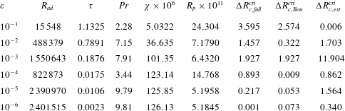
Comparisons between the critical concentration Rayleigh number obtained from various reduced temperatures, in which
 $\unicode[STIX]{x0394}R_{c,full}^{cri}=|R_{c,full}^{cri}-R_{c,the}^{cri}|$
,
 $\unicode[STIX]{x0394}R_{c,Bou}^{cri}=|R_{c,Bou}^{cri}-R_{c,the}^{cri}|$
. Here
 $R_{c,full}^{cri}$
is the numerically calculated value from (3.26) to (3.30),
 $R_{c,Bou}^{cri}$
is the numerically calculated value from (3.39) to (3.41), and
 $R_{c,the}^{cri}$
is the theoretical value predicted by (3.54); and
 $\unicode[STIX]{x0394}R_{c,est}^{cri}$
is defined by (3.57). For all cases in this table,
 $L=10$
mm,
 $\unicode[STIX]{x1D6E4}_{1}=0$
and
 $\unicode[STIX]{x1D6E4}_{2}=1$
.

In this section, we present and compare various results of critical concentration Rayleigh number
 $R_{c}^{cri}$
that are predicted by the theoretical criterion, i.e. (3.54), and numerical solutions based on the full equations or Boussinesq equations. Comparisons and discussions are presented from three aspects. Note that in §§ 3.4.1 and 3.4.2, the height of the fluid layer is set as 10 mm, which is a typical length scale in the numerical and experimental studies of natural convection in near-critical pure fluids (Zappoli, Beysens & Garrabos Reference Zappoli, Beysens and Garrabos2016).
3.4.1 Results for different reduced temperatures
Numerical calculations for the critical concentration Rayleigh number
 $R_{c}^{cri}$
are carried out for six cases with different reduced temperatures, and for both the full equations and Boussinesq equations. The cases are summarized in table 4. The reduced temperature considered here varies from
 $10^{-1}$
to
 $10^{-6}$
, where the latter is the dynamic limit for pure
 $\text{CO}_{2}$
below which the hypothesis of a continuous medium may be invalid (Amiroudine et al.
Reference Amiroudine, Bontoux, Larroud, Gilly and Zappoli2001). We apply the dynamic limit of
 $\unicode[STIX]{x1D700}=10^{-6}$
here since the mixture of
 $\text{CO}_{2}$
and
 $\text{C}_{2}\text{H}_{6}$
is dilute.
It is striking that good agreements between
 $R_{c,full}^{cri}$
,
 $R_{c,Bou}^{cri}$
and
 $R_{c,the}^{cri}$
are found in table 4. That is to say, on the one hand, equation (3.54), obtained from the Boussinesq approximation with the modified Rayleigh number, is applicable for near-critical fluids. On the other hand, for the height
 $L=10$
mm, the role of the compressibility in the onset of convection is almost entirely included in the modified Rayleigh number. The current result is consistent with the analysis of Carlès & Ugurtas (Reference Carlès and Ugurtas1999), where a matched asymptotic analysis was applied for RB instability and suggested that the influence of compressibility on convection onset could be ignored as long as the modified Rayleigh number is used.
3.4.2 Results for different boundary conditions
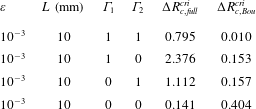
Calculations are also preformed for different boundary conditions, with
 $\unicode[STIX]{x1D700}=0.001$
and
 $L=10$
mm. The results are presented in table 5. Good agreements between the theoretical criterion and numerical results are clearly seen, which suggests that (3.54) is accurate regardless of the boundary condition.
Comparisons between the critical concentration Rayleigh number obtained from different boundary conditions. See the caption of table 4 for the definitions of
 $\unicode[STIX]{x0394}R_{c,full}^{cri}$
and
 $\unicode[STIX]{x0394}R_{c,Bou}^{cri}$
.

3.4.3 Results for different heights of fluid layer
In order to understand the influence of height
 $L$
on the onset of convection, calculations for critical concentration Rayleigh number are performed for several heights ranging from 2 mm to 100 mm, with
 $\unicode[STIX]{x1D700}=0.001$
,
 $\unicode[STIX]{x1D6E4}_{1}=0$
and
 $\unicode[STIX]{x1D6E4}_{2}=1$
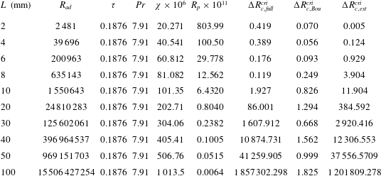
. The results are summarized in table 6. The height
 $L$
has significant effects on the stability. For cases with
 $L\leqslant 10$
mm, the differences between numerical results from full equations and theoretical predictions are small and can be ignored. However, when
 $L>10$
mm, the errors grow dramatically. For example, from
 $L=10$
mm to
 $100$
mm, the height increases tenfold, but the order of magnitude of
 $\unicode[STIX]{x0394}R_{c,full}^{cri}$
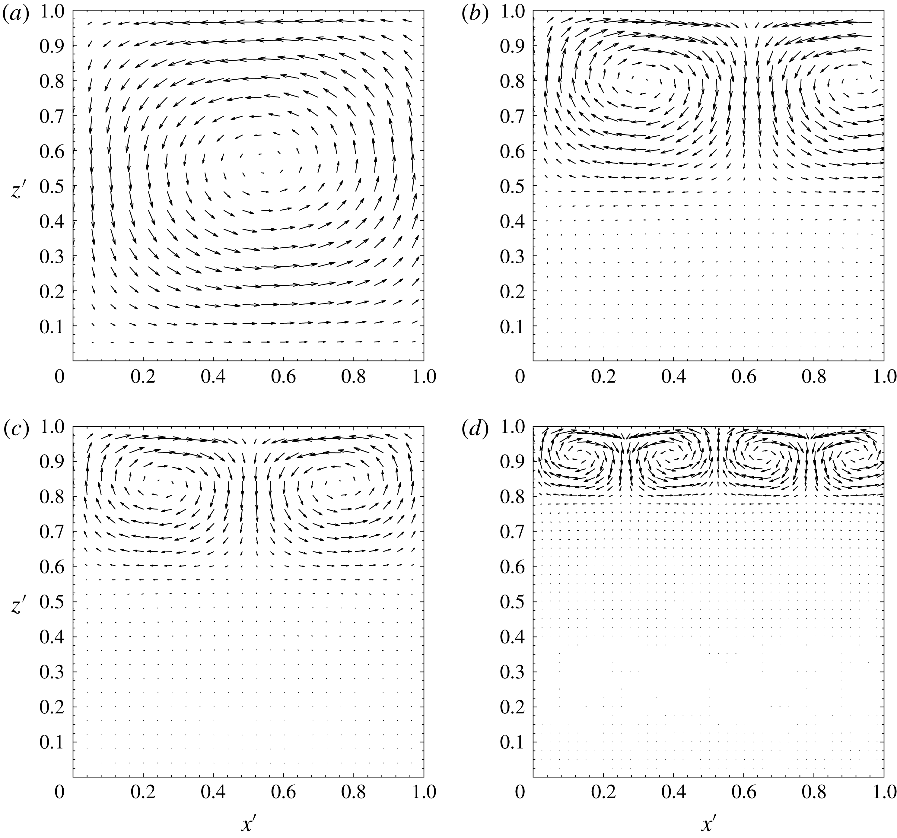
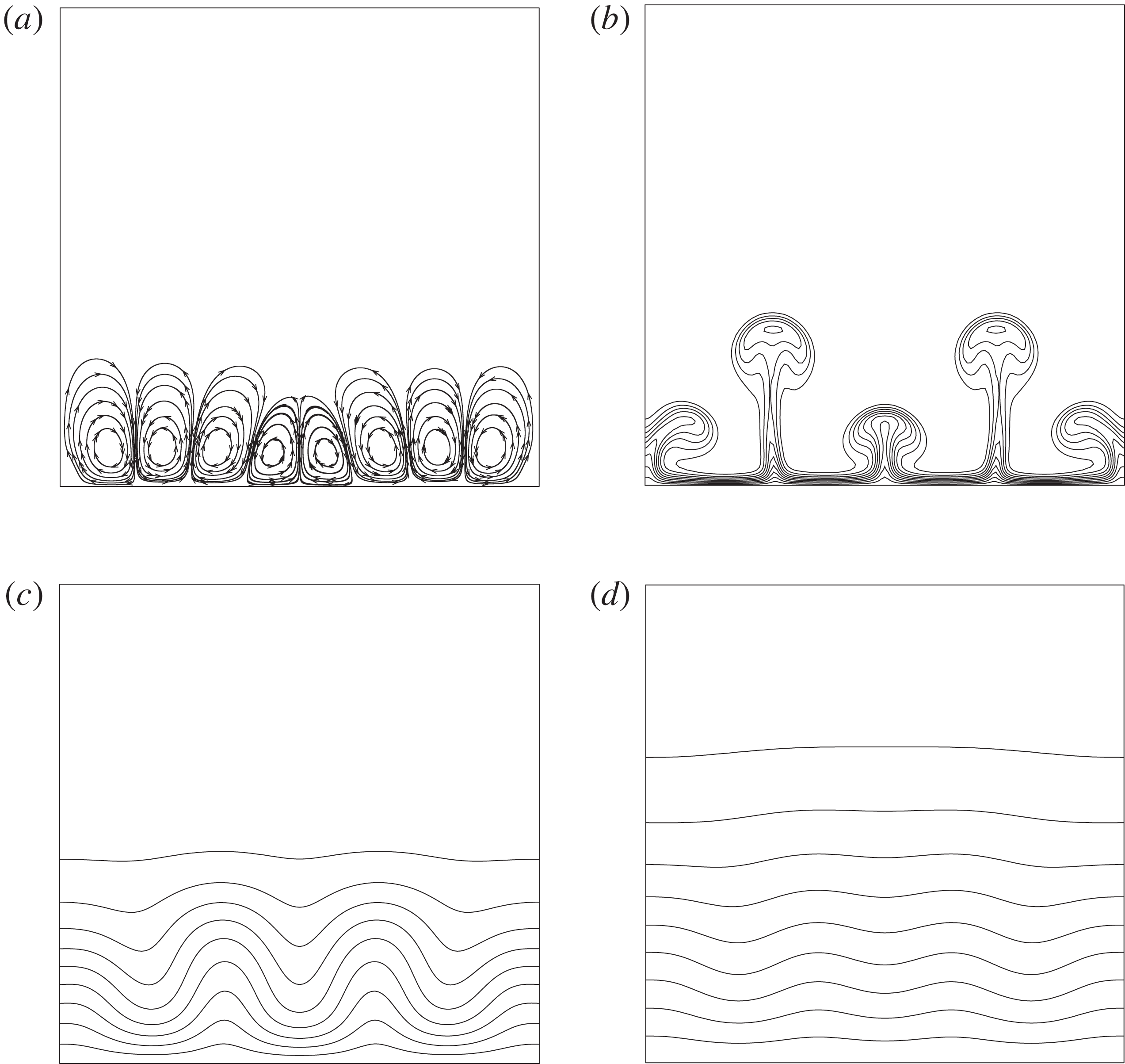
in table 6 increases from 1 to 6. Equation (3.54) is no longer accurate. In addition, we plot in figure 2 the flow fields at the onset of convection under different
 $L$
. As illustrated in figure 2(a), for
 $L=10$
mm, convection is triggered in the whole domain, which is the same as those predicted by Boussinesq equations. However, as
 $L$
increases, the upper part of the domain becomes more unstable than the lower part, because the lower part is nearly motionless (see figure 2
b,c). Finally, for
 $L=100$
mm, the convection is confined in a small region close to the upper boundary (see figure 2
d).
Comparisons between the critical concentration Rayleigh number for various heights. For all cases in this table,
 $\unicode[STIX]{x1D700}=0.001$
,
 $\unicode[STIX]{x1D6E4}_{1}=0$
and
 $\unicode[STIX]{x1D6E4}_{2}=1$
; and
 $\unicode[STIX]{x0394}R_{c,est}^{cri}$
is defined in (3.57). See the caption of table 4 for the definitions of
 $\unicode[STIX]{x0394}R_{c,full}^{cri}$
and
 $\unicode[STIX]{x0394}R_{c,Bou}^{cri}$
.

The influence of height
 $L$
on the flow structures, with (a)
 $L=10$
mm, (b)
 $L=40$
mm, (c)
 $L=50$
mm and (d)
 $L=100$
mm. For all cases here,
 $\unicode[STIX]{x1D700}=0.001$
,
 $\unicode[STIX]{x1D6E4}_{1}=0$
and
 $\unicode[STIX]{x1D6E4}_{2}=1$
.

Now we give our explanations for the phenomenon presented above. The Boussinesq approximation assumes
 $\unicode[STIX]{x1D712}=R_{p}=0$
and
 $\bar{\unicode[STIX]{x1D70C}}^{\prime }=1$
. Therefore, the differences between the results from the full equations and Boussinesq equations must originate from these three factors. In fact, since the influences of
 $\unicode[STIX]{x1D712}$
and
 $R_{p}$
are global, they should not dominate the changes of local flow structures shown in figure 2. Therefore, the non-uniform initial density
 $\bar{\unicode[STIX]{x1D70C}}^{\prime }$
should be the key factor. For all cases considered in this study, the density decreases upwards at neutral stability, which conforms to the theory of double-diffusive convection (Turner Reference Turner1973). The
 $z$
dependence of
 $\bar{\unicode[STIX]{x1D70C}}$
causes the actual thermal diffusivity, defined as
 $D_{T}^{\ast }=\unicode[STIX]{x1D706}/(\bar{\unicode[STIX]{x1D70C}}c_{p})$
, to be a variable. As a result, the actual diffusivity ratio, defined by
 $$\begin{eqnarray}\unicode[STIX]{x1D70F}^{\ast }={\displaystyle \frac{D}{D_{T}^{\ast }}}=\bar{\unicode[STIX]{x1D70C}}^{\prime }\unicode[STIX]{x1D70F},\end{eqnarray}$$
decreases with
 $z^{\prime }$
. According to (3.54), the critical Rayleigh number is proportional to
 $\unicode[STIX]{x1D70F}$
. In other words, the smaller the
 $\unicode[STIX]{x1D70F}$
is, the more unstable the fluid is. Consequently, the fluid close to the upper wall first become unstable as
 $R_{c}$
increases.
After explaining the influence of initial density stratification, the following question then arises. How can we check the applicability of the theoretical criterion? To answer this question, we need to predict the deviation
 $\unicode[STIX]{x0394}R_{c,full}^{cri}$
. Assuming the theoretical criterion still holds locally, based on the aforementioned arguments, the critical concentration Rayleigh number for convection onset can be roughly estimated as
 $$\begin{eqnarray}R_{c,est}^{cri}=\unicode[STIX]{x1D70F}_{min}^{\ast }(R^{cri}+R_{ad})=\bar{\unicode[STIX]{x1D70C}}^{\prime }(z^{\prime }=1)\unicode[STIX]{x1D70F}(R^{cri}+R_{ad}),\end{eqnarray}$$
where
 $R_{c,est}^{cri}$
is the estimated critical concentration Rayleigh number, and
 $\unicode[STIX]{x1D70F}_{min}^{\ast }$
is the minimum value of
 $\unicode[STIX]{x1D70F}^{\ast }$
. From hydrostatic relationships,
 $\bar{\unicode[STIX]{x1D70C}}^{\prime }(z^{\prime }=1)\approx 1-(\unicode[STIX]{x1D712}-R_{p}R_{c})/2$
. The deviation from the theoretical criterion is our main concern, which is thus given by
 $$\begin{eqnarray}\unicode[STIX]{x0394}R_{c,est}^{cri}=R_{c}^{cri}-R_{c,est}^{cri}={\textstyle \frac{1}{2}}\unicode[STIX]{x1D70F}(R^{cri}+R_{ad})[\unicode[STIX]{x1D712}-\unicode[STIX]{x1D70F}R_{p}(R^{cri}+R_{ad})].\end{eqnarray}$$
Calculations for
 $\unicode[STIX]{x0394}R_{c,est}^{cri}$
are carried out for all cases in tables 6 and 4. By comparing
 $\unicode[STIX]{x0394}R_{c,full}^{cri}$
and
 $\unicode[STIX]{x0394}R_{c,est}^{cri}$
, it turns out that (3.57) can give rough estimates for the deviation from the theoretical criterion. Therefore, (3.57) can be applied to check the applicability of (3.54).
In conclusion, when the height of the fluid layer
 $L$
is small (less than 10 mm for this study), the initial density stratification is negligible, and the criterion for the onset of convection obtained from the Boussinesq approximation is accurate for near-critical cases, which is given by
 $$\begin{eqnarray}R_{c}\geqslant R_{c}^{cri}=\unicode[STIX]{x1D70F}(R^{cri}+R_{ad}),\end{eqnarray}$$
where
 $R^{cri}$
is the critical Rayleigh number in thermal RB instability. The accuracy of (3.58) is influenced by initial density stratification. When
 $L$
increases, the upward-decreasing initial density makes the upper part of domain become more unstable by reducing the actual diffusivity ratio, and the actual critical concentration Rayleigh number is less than the theoretical one. The deviation can be roughly estimated by (3.57). In later sections of this paper, we consider cases with
 $L$
less than 10 mm to guarantee the validity of (3.58).
3.5 Discussions about the criterion
From (3.58) and the definitions of the non-dimensional numbers, we obtain the critical concentration difference above which convection occurs,
 $$\begin{eqnarray}\unicode[STIX]{x1D6FF}_{c,onset}={\displaystyle \frac{\unicode[STIX]{x1D702}D}{\unicode[STIX]{x1D70C}_{c}g\unicode[STIX]{x1D705}L^{3}}}R^{cri}+{\displaystyle \frac{\unicode[STIX]{x1D6FD}DL}{\unicode[STIX]{x1D705}D_{T}}}\unicode[STIX]{x1D735}_{ad},\end{eqnarray}$$
which is a function of the physical properties (closely related to the proximity to the critical point) and
 $L$
. The first term on the right-hand side of (3.59) corresponds to the contribution of the Rayleigh criterion, whereas the second term corresponds to the contribution of the adiabatic temperature gradient
 $\unicode[STIX]{x1D735}_{ad}$
, also known as the Schwarzschild criterion.
The critical concentration difference, given by (3.59), as a function of the reduced temperature (along the critical isochore
 $\unicode[STIX]{x1D70C}=\unicode[STIX]{x1D70C}_{c}$
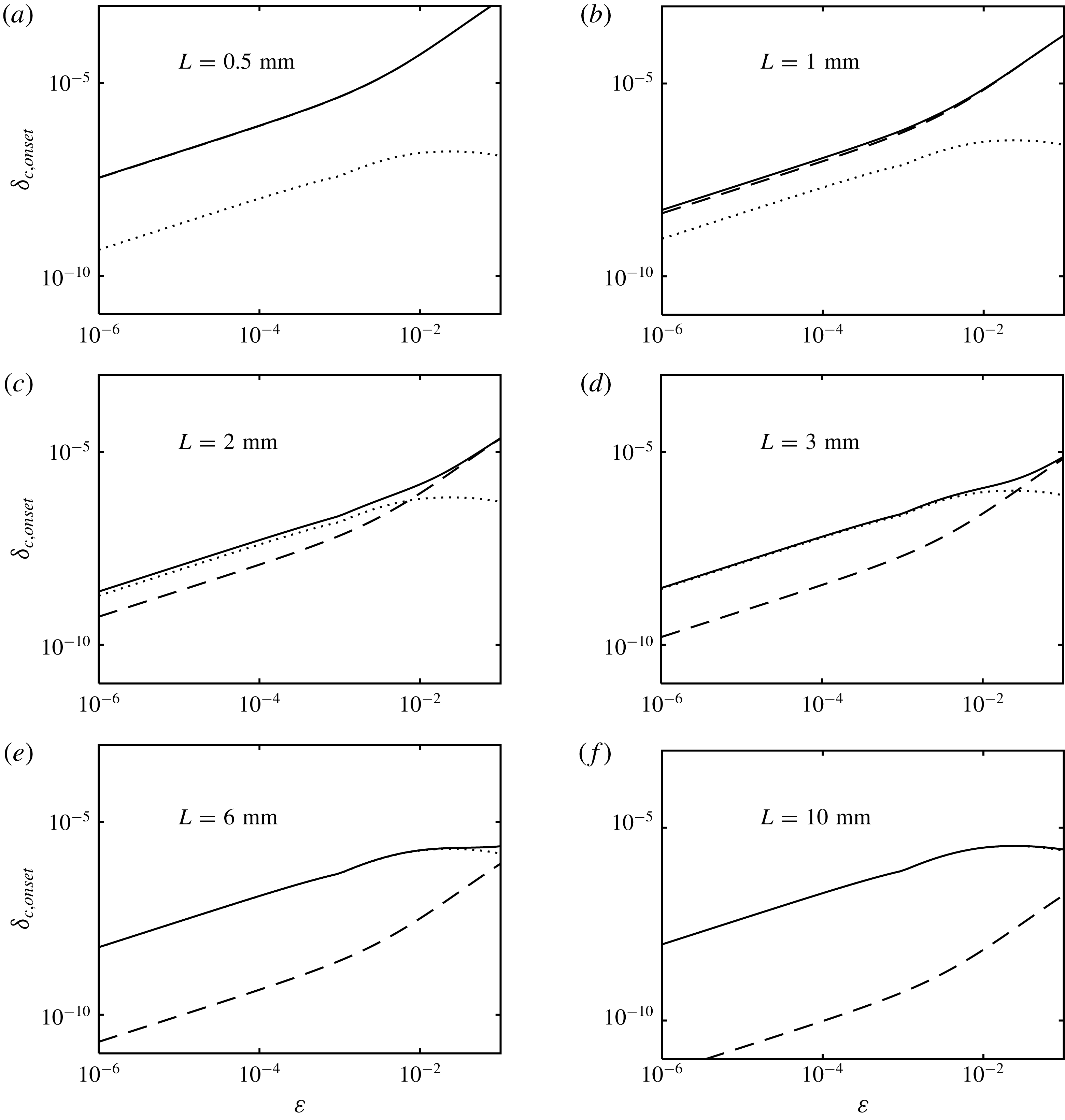
) for several values of the height, ranging from 0.5 mm to 10 mm. Solid curve, total
 $\unicode[STIX]{x1D6FF}_{c,onset}$
calculated from (3.59); dashed curve, Rayleigh part of
 $\unicode[STIX]{x1D6FF}_{c,onset}$
; dotted curve, Schwarzschild part of
 $\unicode[STIX]{x1D6FF}_{c,onset}$
. Note that the dashed curve coincides with the solid curve in (a), and the dotted curve coincides with the solid curve in (f).

We plot in figure 3 the critical concentration difference as a function of
 $\unicode[STIX]{x1D700}$
for several values of the height
 $L$
ranging from 0.5 mm to 10 mm. To understand the roles of the two different criteria, their individual contributions are also plotted in figure 3 with different line styles, dashed line for Rayleigh term and dotted line for Schwarzschild term. It shows that both the Rayleigh term and the Schwarzschild term are highly dependent on
 $\unicode[STIX]{x1D700}$
, tending to zero close to the critical point. Furthermore, the relative importance of the two criteria is closely linked to both the height of the fluid layer and the distance to the critical point. Specifically, if
 $L$
is small, according to figures 3(a) and 3(b), the onset of convection is almost solely governed by the Rayleigh criterion, in which the concentration difference given by the Schwarzschild criterion is negligible. As
 $L$
continues to increase, the dominance of Rayleigh criterion only holds in a distance away from the critical point, and there is a transition from Rayleigh criterion to Schwarzschild criterion when
 $\unicode[STIX]{x1D700}$
tends to zero. In figure 3(c,d), such a transition occurs around
 $\unicode[STIX]{x1D700}=0.01$
. Finally, as shown in figure 3(e,f), when
 $L$
is large, the transition between the two criteria occurs far away from the critical point (
 $\unicode[STIX]{x1D700}>0.1$
), and the onset of convection is almost solely governed by the Schwarzschild criterion in the near-critical region.
The behaviour introduced above is different from that in the context of RB convection (Carlès & Ugurtas Reference Carlès and Ugurtas1999). In RB instability of near-critical fluids, the critical temperature difference tends to a constant instead of zero as the critical point is approached. Besides, the onset of convection is always governed by the Rayleigh criterion far from the critical point, and by the Schwarzschild criterion close to the critical point.
Moreover, the mechanism of instability is also different from that of RB instability. According to the theory of double-diffusive convection (Radko Reference Radko2013), the instability originates from the difference in rates of diffusion between heat and mass, which can be interpreted as follows. When moving a small parcel of fluid (small perturbation) upwards (downwards), it expands (is compressed) due to the hydrostatic pressure with a temperature decrease (increase). Now the parcel is cooler (hotter) along with a higher (lower) concentration than the surrounding fluid. Since heat diffusion is faster than mass diffusion (
 $\unicode[STIX]{x1D70F}<1$
), it adjusts its temperature quickly to the surrounding one. Finally, the parcel of fluid is lighter (heavier) than the surroundings, and continues to move so long as there is a vertical gradient of concentration to supply potential energy (Turner Reference Turner1973). In this way, the instability can occur under a statically stable state. However, for RB instability, only heat diffusion is involved and a density distribution which increases upwards is necessary for instability.
4 Application to a transient natural convection problem
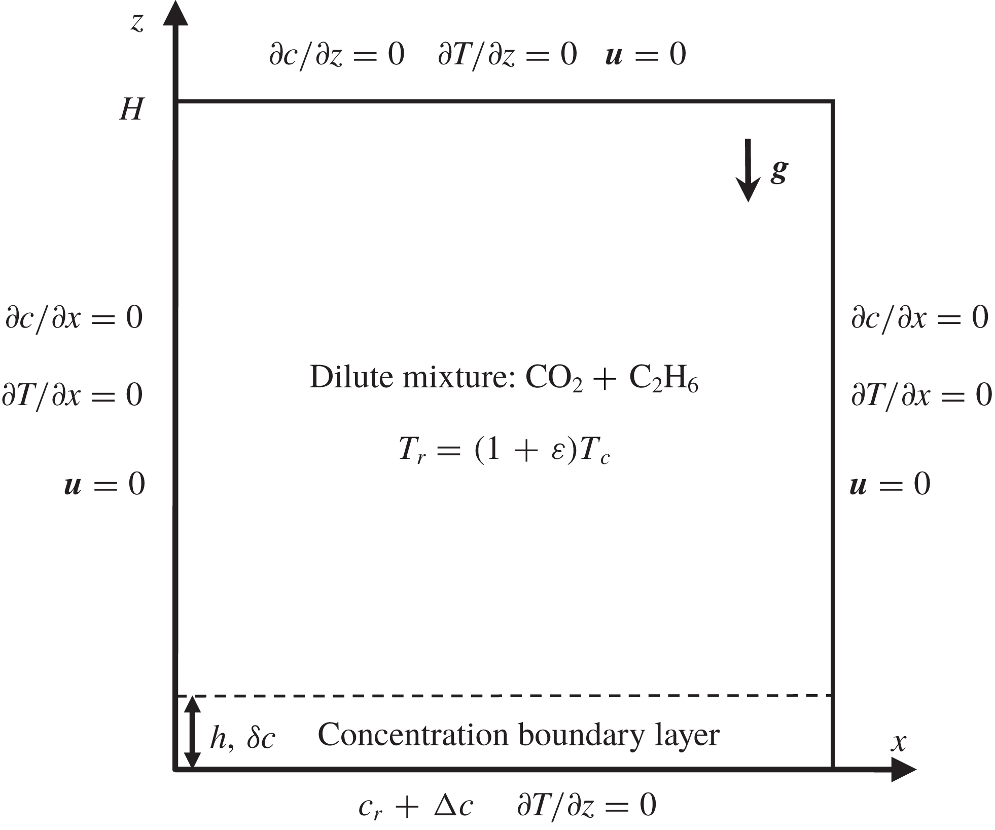
In this section, we apply the criterion developed in the previous section to interpret the onset of convection in a square cavity driven by an increase of concentration at the lower boundary. The physical model is shown in figure 4. We consider a two-dimensional square cavity of height
 $H=10$
mm filled with a dilute near-critical binary fluid mixture of
 $\text{CO}_{2}$
and
 $\text{C}_{2}\text{H}_{6}$
, with the initial concentration
 $c_{r}$
of
 $\text{C}_{2}\text{H}_{6}$
equalling 0.005. The fluid is initially motionless, homogeneous, stratified around critical density
 $\unicode[STIX]{x1D70C}_{c}$
and at thermodynamic equilibrium (
 $T=T_{r}$
, with
 $T_{r}$
the reference temperature). Also, the initial density
 $\bar{\unicode[STIX]{x1D70C}}$
and reference pressure
 $p_{ref}$
satisfy the condition of static equilibrium with the constraint of a mean density equal to
 $\unicode[STIX]{x1D70C}_{c}$
(see (2.2)).
The two-dimensional physical model for the transient natural convection problem.

The concentration at the bottom wall is slightly increased by
 $\unicode[STIX]{x0394}c$
suddenly from its initial value
 $c_{r}$
. We assume
 $\text{C}_{2}\text{H}_{6}$
is the only species transported through the bottom wall. The other three walls are no-slip, impermeable and all the walls are thermally insulated. The boundary condition for concentration employed in this study is often encountered in chemical extraction processes. In these processes, a solute dissolves into a near-critical/supercritical solvent from a solid substrate, and
 $\unicode[STIX]{x0394}c$
is the difference between the actual concentration and the solubility. The resulting mixture is often dilute since the solubility is usually small.
4.1 Basic phenomena and configuration
We investigate the onset of convection in a two-dimensional cavity filled with a near-critical
 $\text{C}_{2}\text{H}_{6}$
–
 $\text{CO}_{2}$
mixture under gravity by suddenly increasing the concentration of the bottom plate by
 $\unicode[STIX]{x0394}c$
from its initial value
 $c_{r}$
. However, our recent pioneering work (under review) reveals that the PE can also be induced by concentration gradients, whose basic mechanism is described as follows. After concentration at the bottom wall increases, due to the vanishing diffusion coefficient, a thin concentration boundary layer (CBL) forms along the bottom wall, which expands upwards strongly because of the large concentration expansion coefficient. In this way, the boundary layer acts like a piston which drives a compression wave in the bulk fluid. The compression wave flashes back and forth in the cavity, leading to a homogeneous heating and a uniform increase of pressure in the whole domain. Above all, the PE caused by concentration is a fast energy equilibrium mechanism. The concentration field is still relaxed through diffusion, and the concentration difference in the boundary layer is constant. In other words, the PE here has slight influence on the onset of convection, since the buoyancy is still governed by concentration difference. However, in the thermal RB problem of near-critical pure fluids, unlike the PE caused by concentration, the thermal PE makes the temperature difference in the boundary layer decrease with time, which thus has strong influences on the onset of convection.
As shown in figure 4, the domain consists of a homogeneous bulk fluid and a CBL along the bottom plate with a thickness
 $h$
(or mean thickness when the CBL is deformed by convection vortices) growing at the speed of diffusion. The thickness of the CBL is evaluated as the distance to the bottom plate where the local concentration reaches the bulk one with a relative difference less than 1 %. Accordingly, the concentration difference in the CBL is
 $\unicode[STIX]{x1D6FF}c=0.99\unicode[STIX]{x0394}c$
. The CBL merges with the bulk fluid at its upper edge, corresponding to a free boundary governed by continuity (Amiroudine et al.
Reference Amiroudine, Bontoux, Larroud, Gilly and Zappoli2001). The bulk fluid features homogeneous concentration and temperature fields, along with a stratified density field caused by the hydrostatic effect. Besides, the temperature and pressure in the whole domain increase homogeneously due to the PE. During the development of the CBL, when
 $\unicode[STIX]{x1D6FF}c$
exceeds its threshold value, the CBL becomes unstable and convection occurs. Above all, the CBL is a laterally bounded horizontal layer of near-critical binary fluid mixture with vertical negative concentration gradient. The upper boundary of the CBL is approximately stress-free, while the lower boundary is rigid. This part of the study is devoted to applying the criterion developed in the previous section to interpret the behaviour of the CBL for different values of
 $\unicode[STIX]{x0394}c$
.
4.2 Acoustic filtering and numerical approach
When solving (2.5)–(2.9), the time step should be quite small to guarantee numerical stability (Zappoli et al. Reference Zappoli, Amiroudine, Carles and Ouazzani1996), which is actually governed by acoustic phenomena. However, currently we are interested in the onset of convection, namely the stability of the CBL, so the descriptions of the flow field on an acoustic time scale are not needed. Therefore, the acoustic filtering procedure (also called low-Mach-number approximation) is utilized to reduce the computation time. The acoustic filtering was originally developed by Paulucci (Reference Paulucci1982) for a perfect gas, in which the density stratification is insignificant. An improved acoustic filtering proposed by Accary et al. (Reference Accary, Raspo, Bontoux and Zappoli2005a ) is employed in this study, which takes into account the appreciable density stratification in near-critical fluids caused by gravity. The basic procedures of acoustic filtering are normalizing the variables, expanding the dimensionless variables in series of Mach number (a small value) and writing the equations to the leading order (Zappoli et al. Reference Zappoli, Amiroudine, Carles and Ouazzani1996; Shen & Zhang Reference Shen and Zhang2012). For the sake of brevity, these procedures are not detailed in this paper. One can refer to the paper of Shen & Zhang (Reference Shen and Zhang2012) for more details. The governing equations after acoustic filtering are written as
 $$\begin{eqnarray}\displaystyle & \displaystyle {\displaystyle \frac{\unicode[STIX]{x2202}\unicode[STIX]{x1D70C}}{\unicode[STIX]{x2202}t}}+\unicode[STIX]{x1D735}\boldsymbol{\cdot }(\unicode[STIX]{x1D70C}\boldsymbol{u})=0, & \displaystyle\end{eqnarray}$$
 $$\begin{eqnarray}\displaystyle & \displaystyle \unicode[STIX]{x1D70C}\left[{\displaystyle \frac{\unicode[STIX]{x2202}\boldsymbol{u}}{\unicode[STIX]{x2202}t}}+(\boldsymbol{u}\boldsymbol{\cdot }\unicode[STIX]{x1D735})\boldsymbol{u}\right]=-\unicode[STIX]{x1D735}p_{dyn}+\unicode[STIX]{x1D702}\unicode[STIX]{x1D6FB}^{2}\boldsymbol{u}+{\displaystyle \frac{1}{3}}\unicode[STIX]{x1D702}\unicode[STIX]{x1D735}(\unicode[STIX]{x1D735}\boldsymbol{\cdot }\boldsymbol{u})+(\unicode[STIX]{x1D70C}-\bar{\unicode[STIX]{x1D70C}})\boldsymbol{g}, & \displaystyle\end{eqnarray}$$
 $$\begin{eqnarray}\displaystyle & \displaystyle {\displaystyle \frac{\unicode[STIX]{x2202}T}{\unicode[STIX]{x2202}t}}+\boldsymbol{u}\boldsymbol{\cdot }\unicode[STIX]{x1D735}T+\unicode[STIX]{x1D735}_{ad}{\displaystyle \frac{\bar{\unicode[STIX]{x1D70C}}}{\unicode[STIX]{x1D70C}}}w={\displaystyle \frac{\unicode[STIX]{x1D706}}{\unicode[STIX]{x1D70C}c_{p}}}\unicode[STIX]{x1D6FB}^{2}T+{\displaystyle \frac{\unicode[STIX]{x1D735}_{ad}}{\unicode[STIX]{x1D70C}g}}{\displaystyle \frac{\unicode[STIX]{x2202}p_{th}}{\unicode[STIX]{x2202}t}}, & \displaystyle\end{eqnarray}$$
 $$\begin{eqnarray}\displaystyle & \displaystyle {\displaystyle \frac{\unicode[STIX]{x2202}c}{\unicode[STIX]{x2202}t}}+\boldsymbol{u}\boldsymbol{\cdot }\unicode[STIX]{x1D735}c={\displaystyle \frac{D}{\unicode[STIX]{x1D70C}}}\unicode[STIX]{x1D735}\boldsymbol{\cdot }(\unicode[STIX]{x1D70C}\unicode[STIX]{x1D735}c), & \displaystyle\end{eqnarray}$$
 $$\begin{eqnarray}\displaystyle & \displaystyle \unicode[STIX]{x1D70C}=\bar{\unicode[STIX]{x1D70C}}+\unicode[STIX]{x1D70C}_{c}[\unicode[STIX]{x1D6FC}p_{th}-\unicode[STIX]{x1D6FD}(T-T_{r})-\unicode[STIX]{x1D705}(c-c_{r})]. & \displaystyle\end{eqnarray}$$
One important result of acoustic filtering is the decomposition of pressure (Accary & Raspo Reference Accary and Raspo2006):
 $$\begin{eqnarray}p=p_{th}+p_{dyn}.\end{eqnarray}$$
Here
 $p_{th}$
is the thermodynamic pressure, which depends only on time representing the cumulative effect of the PE;
 $p_{dyn}$
is the dynamic pressure, which is dependent on space and time and acts to balance inertia and time-varying external forces. The acoustic filtering decouples the dynamic pressure
 $p_{dyn}$
from the density (the EOS). The other result of the acoustic filtering is omitting the viscous dissipation term
 $\unicode[STIX]{x1D6F7}$
in (2.7).
Mathematically, the initial and boundary conditions are given as follows:
 $$\begin{eqnarray}\left.\begin{array}{@{}c@{}}t=0:\quad \bar{T}=T_{r}=(1+\unicode[STIX]{x1D700})T_{c},\quad \bar{c}=c_{r}=0.005,\quad \bar{u}=\bar{w}=0,\\ \displaystyle \bar{\unicode[STIX]{x1D70C}}={\displaystyle \frac{\unicode[STIX]{x1D70C}_{c}gH/K}{1-\text{e}^{-gH/K}}}\text{e}^{-gz/K},\quad \bar{p}_{dyn}=0,\quad \bar{p}_{th}=0,\end{array}\right\}\end{eqnarray}$$
 $$\begin{eqnarray}\left.\begin{array}{@{}c@{}}\displaystyle z=0:\quad {\displaystyle \frac{\unicode[STIX]{x2202}T}{\unicode[STIX]{x2202}z}}=0,\quad c=c_{r}+\unicode[STIX]{x0394}c,\quad u=0,\quad w=-{\displaystyle \frac{D}{1-c}}{\displaystyle \frac{\unicode[STIX]{x2202}c}{\unicode[STIX]{x2202}z}},\\ z=H:\quad {\displaystyle \frac{\unicode[STIX]{x2202}T}{\unicode[STIX]{x2202}z}}={\displaystyle \frac{\unicode[STIX]{x2202}c}{\unicode[STIX]{x2202}z}}=u=w=0,\\ \displaystyle x=0,~x=H:\quad {\displaystyle \frac{\unicode[STIX]{x2202}T}{\unicode[STIX]{x2202}x}}={\displaystyle \frac{\unicode[STIX]{x2202}c}{\unicode[STIX]{x2202}x}}=u=w=0,\end{array}\right\}\end{eqnarray}$$
where the parameter
 $K$
is computed as
 $K=\unicode[STIX]{x1D70C}_{c}^{-1}\unicode[STIX]{x1D6FC}^{-1}$
.
Equations (4.1)–(4.5) with initial and boundary conditions were solved by a finite volume discretization implemented based on OpenFOAM, an open-source C++ library. The pressure–velocity coupling is treated through a block-coupled algorithm (Darwish, Sraj & Moukalled Reference Darwish, Sraj and Moukalled2009). The method is second-order accurate in space: a second-order limited central difference scheme is used for convection terms while a second-order central difference is used for the discretization of the diffusion terms. The method is first-order accurate in time by using an implicit Euler scheme for time integration. The Rhie–Chow interpolation is used to maintain the pressure–velocity coupling on collocated grids and remove oscillations in the solutions. In order to reduce computational time, the convective terms in (4.3) and (4.4) are evaluated using the explicit second-order Adams–Bashforth scheme (Ouazzani & Garrabos Reference Ouazzani and Garrabos2013), which decouples at each time step the energy equation, the concentration equation and the EOS from the momentum and continuity equations. At each time step, the thermodynamic pressure is updated through an overall density balance,
 $$\begin{eqnarray}p_{th}={\displaystyle \frac{\displaystyle \int \unicode[STIX]{x1D70C}\,\text{d}V-\displaystyle \int \bar{\unicode[STIX]{x1D70C}}\,\text{d}V+\displaystyle \int \unicode[STIX]{x1D70C}_{c}[\unicode[STIX]{x1D6FD}(T-T_{r})+\unicode[STIX]{x1D705}(c-c_{r})]\,\text{d}V}{\displaystyle \int \unicode[STIX]{x1D6FC}\unicode[STIX]{x1D70C}_{c}\,\text{d}V}},\end{eqnarray}$$
which is obtained by integrating (2.9) over the whole domain
 $V$
. More details about the numerical method can be found in Hu & Zhang (Reference Hu and Zhang2017).
A non-uniform wall-refined grid is used, and numerical accuracy and stability are tested carefully in terms of time step and grid spacing. We consider graded meshes of
 $105\times 105$
to
 $237\times 237$
in which approximately 40 % of the mesh comprises points inside the near-boundary region (approximately 0.5 mm to the walls), while a uniform mesh is employed in the rest of the domain. The mesh size near the walls is
 $1\times 10^{-4}$
mm. The mesh size in the near-boundary region increases according to a geometric progression. Results suggest the grid of
 $205\times 205$
along with a time step of 0.01 s is sufficient to meet the requirement of accuracy at a reasonable computational cost.
The thermodynamic and transport properties of
 $\text{C}_{2}\text{H}_{6}$
–
 $\text{CO}_{2}$
mixture (
 $c_{r}=0.005$
) at
 $\unicode[STIX]{x1D700}=0.003$
along the critical isochore.

In this study,
 $\unicode[STIX]{x1D700}=0.003$
is chosen in all calculations. The physical properties used in the simulations are summarized in table 7.
4.3 Results and discussions
The stability of the CBL is studied numerically for several concentration increases at the bottom wall, 0.00005, 0.00003, 0.00001, 0.000005, 0.000001 and 0.0000004. Comparisons between numerical results and the stability criterion are made and discussed in this section. The height of the fluid layer
 $L$
and the concentration difference
 $\unicode[STIX]{x0394}c$
in the criterion correspond to the thickness of the CBL
 $h$
and its concentration difference
 $\unicode[STIX]{x1D6FF}c$
, respectively. The upper boundary is stress-free while the lower boundary is rigid. In this study,
 $h$
is evaluated as the distance to the bottom wall where the local concentration reaches the bulk one with a relative difference less than 1 %. Thus,
 $\unicode[STIX]{x1D6FF}c$
equals
 $0.99\unicode[STIX]{x0394}c$
, with
 $\unicode[STIX]{x0394}c$
the concentration increase at the bottom wall. When the CBL is deformed by convection vortices,
 $h$
is the mean thickness in the horizontal direction (Accary et al.
Reference Accary, Raspo, Bontoux and Zappoli2005c
). The physical coefficients in the expressions of the criterion are obtained from table 7.
The convection onset is indicated by a rapid increase in the intensity of convective motion. It is convenient to measure the intensity by introducing the enstrophy field (noted
 $\unicode[STIX]{x1D6FA}$
below), defined by
 $$\begin{eqnarray}\unicode[STIX]{x1D6FA}={\displaystyle \frac{1}{2}}\left({\displaystyle \frac{\unicode[STIX]{x2202}u}{\unicode[STIX]{x2202}z}}-{\displaystyle \frac{\unicode[STIX]{x2202}w}{\unicode[STIX]{x2202}x}}\right)^{2}.\end{eqnarray}$$
In order to identify the instant of convection onset, the evolution of mean enstrophy
 $\overline{\unicode[STIX]{x1D6FA}}$
in the CBL as a function of time for different boundary conditions is shown in figure 5. We define the instant of convection onset as the time after which the mean enstrophy begins to increase exponentially (Accary et al.
Reference Accary, Raspo, Bontoux and Zappoli2005d
). The instants of convection onset are denoted as the symbols ▵ on the curves in figure 5. The vortex structure during the stage of exponential increase is presented in figure 6(a), where eight symmetrical cells fill the CBL. The rotation of the cells alternates from clockwise to anticlockwise horizontally from left to right. It should be noted that the CBL is always stable for
 $\unicode[STIX]{x0394}c=0.0000004$
, since there is no exponential increase in the evolution of mean enstrophy. And the variations in its enstrophy are actually caused by the resistance (no slip) imposed by the sidewalls. Another piece of evidence is that no regular vortex pattern is observed in the CBL.
Time evolutions of the mean enstrophy in the CBL for different boundary conditions. The numbers denote the increments in concentration at the bottom wall. The symbol ▵ represents the onset of convection, namely the mean enstrophy beginning to increase exponentially. The symbol ▫ represents the collapse of the CBL caused by intense convective vortices (see figure 8). The symbol ○ denotes return to stability, namely the time when the mean enstrophy begins to decrease.

(a) Streamlines showing the vortex structure in the CBL after convection onset at
 $t=50$
s for
 $\unicode[STIX]{x0394}c=0.00001$
. (b) Snapshot of the concentration field at
 $t=62$
s for
 $\unicode[STIX]{x0394}c=0.00001$
showing the CBL after its collapse. (c) Snapshot of the concentration field before crossing the Schwarzschild line at
 $t=950$
s for
 $\unicode[STIX]{x0394}c=0.000001$
. (d) Snapshot of the concentration field after crossing the Schwarzschild line and returning to stability at
 $t=2000$
s for
 $\unicode[STIX]{x0394}c=0.000001$
.

Evolution of the CBL’s thickness for different boundary conditions (horizontal lines from left to right), and the neutral stability curve as directly derived from (3.59). The numbers denote the increments in concentration at the bottom wall. The symbol ▵ represents the onset of convection (see figure 5). The symbol ▫ represents the collapse of the CBL caused by intense convective vortices (see figure 8). The symbol ○ denotes return to stability (see figure 5).

The horizontal lines in figure 7 represent the evolution (from left to right) of the CBL thickness for several values of
 $\unicode[STIX]{x0394}c$
obtained from numerical results. Figure 7 also plots the neutral stability curve, derived from (3.59), which gives the theoretical estimate of critical concentration difference
 $\unicode[STIX]{x1D6FF}c_{onset}$
for a range of
 $h$
. As shown in figure 7, the neutral stability curve comprises two branches, the left branch corresponding to the Rayleigh criterion and the right branch corresponding to the Schwarzschild criterion. The neutral stability line suggests that the whole domain can be divided into two parts: the unstable zone above it and the stable zone below it. The instants for the onset of convection, determined from figure 5, are also marked with symbols ▵ in figure 7. This demonstrates that the theoretical criterion gives good predictions for the onset of convection: as the CBL grows with time by diffusion and crosses the Rayleigh line into the unstable zone, the CBL becomes unstable and the convection onset is detected. Besides, for
 $\unicode[STIX]{x0394}c=0.0000004$
, the evolution curve is always located in the stable zone, so no convection occurs.
Time evolution of the CBL thickness for different boundary conditions. The numbers denote the increments in concentration at the bottom wall. For all cases with
 $\unicode[STIX]{x0394}c\geqslant 0.000005$
, each symbol ▫ refers to the collapse of the CBL, namely the time when the thickness drops suddenly, caused by intense convective vortices. The symbol ○ denotes return to stability (see figure 5).

For cases of
 $\unicode[STIX]{x0394}c\geqslant 0.000005$
, the growing vortices can produce enough convective motion to cause the deformation of the CBL and its final collapse. As shown in figure 6(b), a feature of the collapse is some concentration plumes rising from the CBL. The time evolution of the CBL’s thickness for different boundary conditions is displayed in figure 8. The instants for the collapse are clearly exhibited, which are denoted as the symbols ▫ in figures 5, 7 and 8.
For the case of
 $\unicode[STIX]{x0394}c=0.000001$
, the convective transport caused by the vortices is too weak to make the CBL collapse. It grows progressively through diffusion with noticeable deformation (see figure 6
c). However, an unexpected stabilizing phenomenon happens around
 $t=951$
s, when the mean enstrophy begins to decrease exponentially (see figure 5). We call this phenomenon the return to stability (RTS), which is denoted as the symbol ○ in figures 5, 7 and 8. Afterwards, the convective motion is damped, and the distortion of isoconcentration lines in the CBL fades out gradually, as shown in figure 6(d).
However, it is demonstrated in figure 7 that the symbol ○ for RTS is situated in the unstable region near the Schwarzschild line. From a theoretical point of view, the RTS should not happen until the curve for the evolution of CBL in figure 7 crosses the Schwarzschild line, entering the stable region, as demonstrated by previous work for thermal RB convection (Accary et al.
Reference Accary, Raspo, Bontoux and Zappoli2005c
). In other words, the real system is more stable than what is predicted by the theoretical criterion. We believe that the discrepancy between the numerical result and the theoretical prediction is mainly due to the lateral boundaries of the CBL. Recall that, in the stability analysis, we consider a horizontally infinite fluid layer. But the real CBL is finite with no-slip boundaries on both left and right sides. When
 $h$
is small, the aspect ratio of the CBL is large. The influence of the sidewalls is negligible and the CBL can be approximated as a horizontally infinite fluid layer. That is why the Rayleigh criterion can offer good predictions for the onset of convection. However, when the RTS happens, the aspect ratio is nearly 1.5. The rigid lateral walls provide resistance for the upward motion, and the CBL is more stable than a horizontally unbounded fluid layer. Therefore, the RTS happens before crossing the theoretical Schwarzschild line.
Above all, the criterion developed in the last section can offer good predictions for the stability of the CBL except for the case of RTS. We attribute the discrepancy to lateral walls, which provide resistance and make the CBL more stable than a laterally unbounded fluid layer (the model used in stability analysis).
5 Conclusion
The convective instability induced by a concentration gradient in a horizontal fluid layer of a near-critical binary fluid mixture is investigated numerically. The problem is regarded as a limiting case of double-diffusive convection. Numerical calculations of critical Rayleigh number were carried out for various conditions: reduced temperature, boundary conditions and the height of the fluid layer. Our results suggest that if the initial density stratification is negligible, e.g. when the height of the fluid layer is less than 10 mm, the theoretical criterion developed under the Boussinesq approximation with the modified Rayleigh number (3.58) is accurate for near-critical fluids. However, when the height of the fluid layer is large, the initial density stratification makes the upper part of the domain become more unstable, and the actual critical concentration Rayleigh number is less than the theoretical one. We propose a method to estimate the deviation, which can be used to check the applicability of the theoretical criterion.
Then we apply the criterion to interpret the onset of convection in a model in analogy to the bottom-heating configuration: a near-critical binary fluid mixture confined in a two-dimensional cavity submitted to concentration increases at the bottom wall. The stability of the CBL is studied numerically for several concentration increases at the bottom wall. The numerical results demonstrate four typical behaviours of the CBL: (i) onset of convection, defined as the time when the mean enstrophy of the CBL begins to increase exponentially; (ii) collapse of the CBL, defined as the time when the mean thickness of the CBL drops suddenly, caused by intense convective vortices after the convection onset; (iii) return to stability, namely the time when the mean enstrophy begins to decrease after the exponential increase; and (iv) remaining stable, namely the CBL always being stable without exponential increase in the mean enstrophy. Besides, for different intensities of concentration increases, numerical results reveal that there are three possibilities for evolutions of the CBL: (i) and (ii) for high intensity, (i) and (iii) for moderate intensity, and (iv) for low intensity. Comparisons between numerical results and the stability criterion are made. The consistencies between the numerical results and theoretical criterion are observed expect for the behaviour of return to stability, which is attributed to the resistance provided by lateral walls.
This work is an extension of previous studies on RB convection in near-critical pure fluids. The role of concentration in natural convection within a framework of near-critical binary fluid mixture is elaborated in the current work. In the future, a more accurate modification to the theoretical criterion should be proposed to include the influence of initial density. For the cavity flow problem, a criterion based on a laterally bounded fluid layer should be developed to give more accurate predictions for the stability of the CBL.
Acknowledgements
The support of the National Natural Science Foundation of China (no. 51476001) and the support from Beijing Engineering Research Center of City Heat are gratefully acknowledged. The authors are grateful to the reviewers of the manuscript for their constructive criticisms. We would also thank Professor S. H. Davis for his helpful instructions on this work.