2.1 Avoiding gyroaverages of the electrostatic potential

We consider the simple situation of a two-dimensional single-species plasma in the $xy$ -plane immersed in a constant and uniform magnetic field $\boldsymbol{B}=B_{0}\boldsymbol{e}_{z}$ . We define the gyrofrequency $\unicode[STIX]{x1D6FA}=qB_{0}/m$ , with $q$ the charge of the particles in the plasma, and $m$ their mass. The position of a given particle is $\boldsymbol{r}=\boldsymbol{R}+\unicode[STIX]{x1D746}$ , where $\boldsymbol{R}$ is the guiding centre (or gyrocentre) position, and $\unicode[STIX]{x1D746}$ is the Larmor radius vector $\unicode[STIX]{x1D746}=-\unicode[STIX]{x1D70C}\sin \unicode[STIX]{x1D6FE}\boldsymbol{e}_{x}+\unicode[STIX]{x1D70C}\cos \unicode[STIX]{x1D6FE}\boldsymbol{e}_{y}$ , where $\unicode[STIX]{x1D6FE}$ is the gyroangle and $(\boldsymbol{e}_{x},\boldsymbol{e}_{y},\boldsymbol{e}_{z})$ is the standard Cartesian orthonormal basis of $\mathbb{R}^{3}$ , with $\boldsymbol{e}_{z}$ aligned with the magnetic field. If velocities are normalised to the thermal speed $v_{\text{th}}$ and spatial scales are normalised to the Larmor radius $\unicode[STIX]{x1D70C}_{L}=v_{\text{th}}/\unicode[STIX]{x1D6FA}$ , the gyrokinetic-Poisson equations for the gyrocentre distribution function $f(\boldsymbol{R},\unicode[STIX]{x1D70C},t)$ are given by (Hazeltine & Meiss Reference Hazeltine and Meiss2003; Plunk et al. Reference Plunk, Cowley, Schekochihin and Tatsuno2010)

where

In (2.1), $\langle \cdot \rangle _{\boldsymbol{R}}$ represents the gyroaverage at fixed guiding centre position $\boldsymbol{R}=X\boldsymbol{e}_{x}+Y\boldsymbol{e}_{y}$ :

where $X$ and $Y$ are held fixed. We chose the relatively simple gyrokinetic system of equations (2.1) and (2.2) to better focus on the central question of this paper, namely the fast and accurate evaluation of the averages over the gyroangle $\unicode[STIX]{x1D6FE}$ appearing in both equations. However, the method we present here is applicable to the more general gyrokinetic systems commonly used to study astrophysical and fusion plasmas. We should mention that (2.1) and (2.2) are a surprisingly accurate description of the dynamics of a beam of charged particles in the plane perpendicular to the magnetic field in high intensity cyclotrons (Cerfon et al. Reference Cerfon, Freidberg, Parra and Antaya2013; Guadagni Reference Guadagni2015; Cerfon Reference Cerfon2016). With this application in mind, we want to allow boundary conditions on $\unicode[STIX]{x1D6F7}$ that are not periodic, such as free space boundary conditions for instance.

If one has a numerical method to accurately evaluate $\langle \unicode[STIX]{x1D735}_{\boldsymbol{r}}\unicode[STIX]{x1D6F7}\rangle _{\boldsymbol{R}}$ on the desired numerical grid, then a number of established numerical schemes are available to advance $f$ in time according to (2.1) (Peterson & Hammett Reference Peterson and Hammett2013; Guadagni Reference Guadagni2015). Clearly, the challenge that is specific to gyrokinetics is the numerical evaluation of the gyroaverage for the charge density in (2.2) and of the gyroaveraged potential (2.4) when these quantities are not periodic. In the introduction, we have mentioned popular methods to accomplish this task. We propose a different approach, based on Fourier transforms, which leads to high-order accurate answers. Such an approach is not practical in the current formulation of the problem since $\unicode[STIX]{x1D6F7}$ is not periodic and is unbounded for free space boundary conditions. Our first step therefore consists of casting equations (2.1) and (2.2) in a form which is compatible with a Fourier representation.

For our simple geometry, $\unicode[STIX]{x1D735}_{\boldsymbol{r}}=\unicode[STIX]{x1D735}_{\boldsymbol{R}}$ , so it is straightforward to re-express (2.1) and (2.2) in terms of equations for quantities which only depend on the guiding centre position $(X,Y)$ :

where we also made use of the fact that the gradient operator commutes with the gyroaveraging operator (Guadagni Reference Guadagni2015). Since $\unicode[STIX]{x1D6F7}$ is not periodic and unbounded, it does not have a Fourier transform. Computing $\langle \unicode[STIX]{x1D6F7}\rangle _{\boldsymbol{R}}$ using standard Fourier techniques is therefore not an available option. The idea instead is to define a new potential-like function $\unicode[STIX]{x1D712}(\boldsymbol{R},\unicode[STIX]{x1D70C},t)=\langle \unicode[STIX]{x1D6F7}\rangle _{\boldsymbol{R}}(\boldsymbol{R},\unicode[STIX]{x1D70C},t)$ which we call the gyropotential. The key then is to not evaluate $\unicode[STIX]{x1D712}$ as given by its definition, but instead to see that it is the solution of the Poisson equation

which we obtained by gyroaveraging (2.6) holding the guiding centre position $\boldsymbol{R}$ fixed, and using once more the fact that the gradient operator commutes with the gyroaveraging operator. At this point, we have turned (2.1) and (2.2) into the following new system of equations:

Unsurprisingly, this system shares many similarities with the two-dimensional inviscid Euler equations in vorticity–streamfunction form (Plunk et al. Reference Plunk, Cowley, Schekochihin and Tatsuno2010; Cerfon Reference Cerfon2016). The major difference with the Euler equations is that the term $\langle \tilde{f}\rangle _{\boldsymbol{R}}$ couples the dynamics at different values of $\unicode[STIX]{x1D70C}$ . In the context of the present article, the significant aspect of the system of equations above is that it has the desirable property of only involving gyroaverages of $\tilde{f}$ , which, unlike $\unicode[STIX]{x1D6F7}$ , can be approximated numerically by a compactly supported function. Once $\langle \tilde{f}\rangle _{\boldsymbol{R}}$ is known, Poisson’s equation (2.9) can be solved with standard methods.

It may first seem as if our reformulation of the gyrokinetic Vlasov–Poisson system has a large computational cost because $\unicode[STIX]{x1D712}$ is a function of the variable $\unicode[STIX]{x1D70C}$ . That means that Poisson’s equation (2.9) has to be solved as many times as there are discretisation points for the $\unicode[STIX]{x1D70C}$ variable. In practice, however, this is not a salient issue, for three reasons. First, there exists a wide choice of fast and high-order accurate Poisson solvers with nearly optimal computational complexity. For example, for the free space boundary conditions which are the relevant conditions for beam dynamics in cyclotrons, we may mention the solvers by Jiang et al. (Reference Jiang, Greengard and Bao2014) and by Vico et al. (Reference Vico, Greengard and Ferrando2016), which solve Poisson’s equation on a regular grid in $O(P\log P)$ time, where $P$ is the number of space discretisation points. Second, it is quite common in gyrokinetic simulations to have a very small number ( ${\leqslant}20$ ) of grid points for the $\unicode[STIX]{x1D70C}$ variable (Wilkening et al. Reference Wilkening, Cerfon and Landreman2015; J. Candy, 2016, Private communication). Lastly, the Poisson solve is rarely the rate limiting step in gyrokinetic simulations. This is particularly true for particle-in-cell solvers, in which the particle operations typically dominate the computation and storage requirements (Ricketson & Cerfon Reference Ricketson and Cerfon2017).

2.2 Limitations of a Fourier series expansion

Thus far, we have expressed the gyrokinetic-Poisson system of equations (2.1)–(2.2) in a form that only requires gyroaveraging a function which can be well approximated by a compactly supported function, given by the system of equations (2.8)–(2.9). This allows us to use a Fourier basis to represent that function and to calculate its gyroaverage in Fourier space. 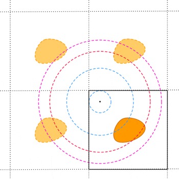However, for problems which are not periodic, despite the compact support of $\tilde{f}$ , a gyroaveraging scheme based on a Fourier series expansion for $\tilde{f}$ can only lead to highly accurate answers under specific conditions. To understand this point, consider the model charge density shown in figure 1. The computational domain is represented by the black box in the lower right corner, and the support of the charge density is shown in orange there. By expanding $\tilde{f}$ in a Fourier basis, one would make the problem periodic, which is represented by the three boxes which are contiguous to the computational domain in figure 1 and represented with dashed lines. Now, consider the four gyroaverages corresponding to different values of $\unicode[STIX]{x1D70C}$ , with common centre the black dot in the upper left corner of the computational domain, and shown in the figure as four dashed circles. The two inner circles, highlighted in blue, give the correct result for the gyroaverage: the average only involves contributions from the true charge density – and no contribution at all for the innermost circle, as it should. However, the two outer circles, highlighted in red, give a false result for the gyroaverage. Along the third circle, the contribution from the true charge density is summed, but so are the contributions from the ‘ghosts’, unphysical charge densities in the contiguous cells. For the outermost circle, corresponding to large $\unicode[STIX]{x1D70C}$ , the average should be zero, but it is not because the ‘ghost’ charge densities contribute to the average.

A possible way to address this issue is to increase the size of the computational domain by padding it with zeroes in such a way that even for the maximum $\unicode[STIX]{x1D70C}$ considered in the simulations, gyrocircles only average the true charge density. This idea is very similar to what is sometimes done to solve Poisson’s equation with a plane wave representation (Genovese et al. Reference Genovese, Deutsch, Neelov, Goedecker and Beylkin2006). It has the clear disadvantage of leading to large computational domains, and therefore significantly more expensive evaluations of the fast Fourier transform (FFT) typically used to calculate the coefficients in the Fourier series.

Now, while a Fourier series expansion leads to the complications discussed above, because it intrinsically implies periodicity for the problem, an expansion on a continuous Fourier basis, i.e. through the Fourier transform, has all the desirable properties for a high-order accurate numerical scheme for gyroaveraging. This is what we discuss in the next section.

Figure 1.

Illustration of the difficulties associated with using a Fourier series representation for computing the gyroaverage of a distribution function $f$ is a non-periodic setting. The computational domain is the box bounded by the continuous lines. The boxes bounded by dashed lines represent some of the boxes induced by the periodicity of the Fourier series representation. The gyroaverage along the blue orbits yield correct results, while the gyroaverage along the red and purple orbits lead to fictitious contributions to the true gyroaverage.

2.3 Fourier and Hankel transform representation

Consider a function $u(\boldsymbol{x},\unicode[STIX]{x1D70C})$ on $\mathbb{R}^{2}\times \mathbb{R}_{{\geqslant}0}$ . The Fourier transform of $u$ with respect to the first two inputs is defined by

The inverse Fourier transform is defined by

Finally, given a real-valued function $u(s)$ defined on $\mathbb{R}_{{\geqslant}0}$ , its Hankel transform of order zero is defined by

where $\text{J}_{0}$ is the Bessel function of the first kind and of order zero. Introducing the gyroaverage at fixed particle position $\boldsymbol{r}=x\boldsymbol{e}_{x}+y\boldsymbol{e}_{y}$ ,

it is well-known that ${\mathcal{F}}\langle f\rangle (\unicode[STIX]{x1D743},\unicode[STIX]{x1D70C},t)=\text{J}_{0}(\unicode[STIX]{x1D70C}\unicode[STIX]{x1D709})({\mathcal{F}}f)(\unicode[STIX]{x1D743},\unicode[STIX]{x1D70C},t)$ . Therefore, we can write

And since we also have the identity

we obtain the desired expression for the only term which needs to be gyroaveraged in the system of equations (2.8)–(2.9):

Note that there is a slight abuse of notation in (2.14)–(2.16) above: in (2.12) we have defined the Hankel transform for functions of a single variable but $({\mathcal{F}}f)$ clearly is not.

Thus, to summarise § 2, we have shown that the gyrokinetic-Poisson system can be rewritten as

All the gyroaveraging operations are contained in the operator ${\mathcal{G}}$ that operates on the function $f$ , which is bounded and has compact support. Furthermore, if $f(X,Y,\unicode[STIX]{x1D70C},t)$ and $\unicode[STIX]{x1D712}(X,Y,\unicode[STIX]{x1D70C},t)$ are known at a given time $t$ , the physical potential $\unicode[STIX]{x1D6F7}(X,Y,t)$ and the number density $n(X,Y,t)$ are given by $\unicode[STIX]{x1D6F7}(X,Y,t)=\unicode[STIX]{x1D712}(X,Y,0,t)$ and $n(X,Y,t)=2\unicode[STIX]{x03C0}{\mathcal{G}}f(X,Y,0,t)$ . In other words, they do not require additional computation, and one just needs to read the values of $\unicode[STIX]{x1D712}(X,Y,\unicode[STIX]{x1D70C},t)$ and $2\unicode[STIX]{x03C0}{\mathcal{G}}f(X,Y,\unicode[STIX]{x1D70C},t)$ corresponding to $\unicode[STIX]{x1D70C}=0$ .

It remains to explain how we discretise $f$ and the operators on the right-hand side of (2.16) in order to evaluate ${\mathcal{G}}f(\boldsymbol{R},\unicode[STIX]{x1D70C},t)$ numerically to high accuracy. This is the purpose of the next section.

3.1 Grid choices

For the design of our numerical scheme, we chose to operate under the constraint that the spatial grid be uniformly spaced. The reason for this is that many of the popular and advanced schemes for both the Vlasov equation and Poisson’s equation are either very difficult to implement on non-uniform grids, or simply do not work on such grids (Shu Reference Shu, Barth and Deconinck1999; Peterson & Hammett Reference Peterson and Hammett2013; Jiang et al. Reference Jiang, Greengard and Bao2014; Vico et al. Reference Vico, Greengard and Ferrando2016). As we will see in §§ 3.2 and 3.4, this constraint leads to computational costs which could have been avoided if we had given ourselves the freedom to use a non-equispaced grid for the spatial variables. Still, even with this constraint and its associated computational cost, the scheme we propose here can be categorised as a fast solver, in the sense that its run-time complexity is $O(K\log K)$ , where $K$ is the number of degrees of freedom in the problem.

In contrast to the spatial grid, we never solve any partial differential equation with respect to either the Fourier space coordinates $(\unicode[STIX]{x1D709}_{x},\unicode[STIX]{x1D709}_{y})$ or the $\unicode[STIX]{x1D70C}$ -coordinate. We take advantage of this fact by using Chebyshev grids for each, which give us access to highly efficient and accurate numerical quadrature schemes.

3.2 The Fourier transform ${\mathcal{F}}$

We start by presenting our method for evaluating ${\mathcal{F}}f$ . For the simplicity of the presentation, we focus on the case in which $f$ depends only on one spatial variable $x$ . The method generalises directly to the two-dimensional tensor grid which we use to compute ${\mathcal{G}}f$ . Consider the function $u$ on $\mathbb{R}$ . Its Fourier transform is

We consider the case in which $u$ is compactly supported on the domain $I=[-a/2,a/2]$ , which is relevant to us, and write $u$ as the exact series

In (3.2), $\mathbf{1}_{I}$ is the indicator function for the interval $I$ , defined by $\mathbf{1}_{I}(x)=1$ if $x\in I$ , and $\mathbf{1}_{I}(x)=0$ otherwise. The Fourier transform of $u$ is then given by

where $\text{sinc}(z)\equiv \sin (\unicode[STIX]{x03C0}z)/(\unicode[STIX]{x03C0}z)$ . We proceed as follows to compute the sum (3.4) in optimal time, with high accuracy, and for values $\unicode[STIX]{x1D709}$ on an arbitrary grid in the Fourier domain. The Fourier coefficients $c_{k}$ are calculated with a straight forward call to the FFT, after discretising $u$ on a uniform grid. The complexity of this operation is $O(N\log N)$ , where $N$ is the number of discretisation points for the $x$ -grid. Once the values of $c_{k}$ are known, we would like to evaluate the sum (3.4) on a $\unicode[STIX]{x1D709}$ -grid which is optimal for the operations which will follow the calculation of ${\mathcal{F}}$ in the evaluation of the full operator ${\mathcal{G}}$ . As mentioned in the previous section, that grid is a non-equispaced Chebyshev grid, which may in addition have different bounds than those naturally induced by the bounds of $I$ in the Fourier transform. To evaluate (3.4), we thus rely on the fast sinc transform (FST) (Greengard et al. Reference Greengard, Lee and Inati2006), which is itself based on the non-uniform fast Fourier transform (NUFFT) (Dutt & Rokhlin Reference Dutt and Rokhlin1993), and which is freely available in a version described in (Greengard & Lee Reference Greengard and Lee2004; Lee & Greengard Reference Lee and Greengard2005). The computational complexity of the FST is $O((N+\hat{N})\log (N+\hat{N}))$ , where $\hat{N}$ is the number of discretisation points for the $\unicode[STIX]{x1D709}$ -grid. For the gyrokinetic-Poisson system (2.17)–(2.18) we are interested in, for which $f$ depends on two spatial variables, this becomes $O((P+\hat{P})\log (P+\hat{P}))$ , where $P\sim N^{2}$ is the total number of spatial grid points and $\hat{P}\sim \hat{N}^{2}$ is the total number of grid points in Fourier space. Since we need to repeat this operation for each value of $\unicode[STIX]{x1D70C}$ , the overall complexity of this step is $O(N_{\unicode[STIX]{x1D70C}}(P+\hat{P})\log (P+\hat{P}))$ , where $N_{\unicode[STIX]{x1D70C}}$ is the number of grid points in velocity space.

Before closing this section, we mention an alternative way of evaluating (3.1) for a compactly supported function $u$ . Since $u$ is compactly supported, it can be viewed as periodic on the domain of integration, so the trapezoidal rule provides a spectrally accurate scheme for the numerical evaluation of the integral (Trefethen & Weideman Reference Trefethen and Weideman2014). The discrete sum resulting from the application of the trapezoidal rule can then be computed with a direct application of the FFT (Pataki & Greengard Reference Pataki and Greengard2011). The issue with this approach is that the number of grid points in real space determines the number of grid points in Fourier space. For most functions of physical interest, the representation in Fourier space is significantly more oscillatory than the representation in real space, so proper resolution in Fourier space requires significant oversampling in real space (Pataki & Greengard Reference Pataki and Greengard2011), which is computationally costly. In contrast, the FST gives us the choice to have a larger number of grid points in Fourier space than the number of grid points we use in real space. Now, since the FST is more expensive than the regular FFT by a constant factor, it can be shown that the run-time complexity of the two approaches is comparable. In our implementations of the scheme we present here, we favour the FST approach because we find the framework in which real space and Fourier space are decoupled elegant, convenient and efficient.

3.3 The Hankel transform ${\mathcal{H}}_{0}$

The next step in the evaluation of ${\mathcal{G}}f$ corresponds to the calculation of the Hankel-like integral

with $\unicode[STIX]{x1D709}=||\unicode[STIX]{x1D743}||$ . Since $\unicode[STIX]{x1D743}$ and $t$ are fixed parameters in this integral, we simplify the notation and consider the computation of the integral

We consider in this work that to the desired numerical accuracy, $\hat{f}$ has compact support in the $\unicode[STIX]{x1D70C}$ -variable. In the context of (3.6), this means that there exists a maximum $\overline{\unicode[STIX]{x1D70C}}$ such that $h=0$ outside the interval $I_{\unicode[STIX]{x1D70C}}=[0,\overline{\unicode[STIX]{x1D70C}}]$ . To compute (3.6) we discretise $I_{\unicode[STIX]{x1D70C}}$ with a Chebyshev grid in $\unicode[STIX]{x1D70C}$ and use Clenshaw–Curtis quadrature, which has geometric convergence for the class of functions we consider here (Trefethen Reference Trefethen2008):

where $N_{\unicode[STIX]{x1D70C}}$ is the number of Chebyshev grid points on the interval $I_{\unicode[STIX]{x1D70C}}$ , the values of $\unicode[STIX]{x1D70C}_{k}$ are the Chebyshev abscissae, and the values of $w_{k}$ are the Clenshaw–Curtis quadrature weights. Now, observe that for fixed computational $\unicode[STIX]{x1D70C}$ - and $\unicode[STIX]{x1D709}$ -grids, the values of $w_{k}\text{J}_{0}(\unicode[STIX]{x1D70C}_{k}\unicode[STIX]{x1D709})\unicode[STIX]{x1D70C}_{k}$ can be precomputed for all $k$ and for all possible values of $\unicode[STIX]{x1D709}$ . Hence, in practice, each individual Hankel integral can be computed as the inner product of one data vector which changes with each time step and one vector of fixed kernel weights. To be more precise, observe that in our case, $h$ is the function ${\mathcal{F}}f$ , which does not only depend on $\unicode[STIX]{x1D70C}$ , but also on $\unicode[STIX]{x1D743}$ and $t$ , as can be seen in (2.14). Letting $h(\unicode[STIX]{x1D743},\unicode[STIX]{x1D70C},t)={\mathcal{F}}f(\unicode[STIX]{x1D743},\unicode[STIX]{x1D70C},t)$ to simplify the notation in the matrices below, all Hankel integrals are computed at once by considering the $N_{\unicode[STIX]{x1D70C}}\times \hat{P}$ matrices $\unicode[STIX]{x1D65D}$ and $\unicode[STIX]{x1D652}$ defined by

and

where $\unicode[STIX]{x1D743}_{j}$ is now viewed as the vector whose components are the coordinates of the $j$ th pair of the $\hat{P}$ Fourier coordinate pairs. Note that $\unicode[STIX]{x1D652}$ is fixed for all time and can be stored after its initial computation. The right-hand side of (2.14), ${\mathcal{H}}_{0}{\mathcal{F}}f(\unicode[STIX]{x1D743},t)$ , is then calculated by computing the entrywise product of $\unicode[STIX]{x1D65D}$ and $\unicode[STIX]{x1D652}$ and summing the columns of that matrix. In mathematical notation, we may write

where $\odot$ represents the Schur product (Davis Reference Davis1962), i.e. entrywise product. The run-time complexity of this operation is $O(N_{\unicode[STIX]{x1D70C}}\hat{P})$ . As a result, when evaluating ${\mathcal{G}}f$ numerically with the method we present here, the total time spent computing Hankel transforms is negligible compared to the total time spent computing forward Fourier transforms.

3.4 The inverse Fourier transform ${\mathcal{F}}^{-1}$

After a straightforward multiplication by $\text{J}_{0}(\unicode[STIX]{x1D70C}\unicode[STIX]{x1D709})$ , all that is left to compute ${\mathcal{G}}f$ is the computation of the inverse Fourier transform ${\mathcal{F}}^{-1}$ . As before, we focus here on the case of the one-dimensional inverse Fourier transform defined by

In principle, this computation can be done with the same numerical tools presented in § 3.2. There are however two key points which we need to revisit. The first point to consider is that we relied on the fact that $u$ was compactly supported (to within the desired numerical accuracy) to reduce the Fourier transform integral to the finite interval $I$ . From the Fourier uncertainty principle (Hardy Reference Hardy1933; Hogan & Lackey Reference Hogan and Lakey2005), it is not clear that the corresponding Fourier transform has numerical compact support on a finite interval of reasonable size. It may first seem as if this observation strongly limits the class of functions for which ${\mathcal{G}}f$ can be accurately computed with our numerical scheme. The functions for which both the Fourier transform and the inverse Fourier transform can be computed without significant loss of accuracy by restricting the quadratures to finite intervals with reasonable sizes are functions which can be represented as a Gaussian distribution function plus a small deviation from the Gaussian behaviour (Hardy Reference Hardy1933; Stein & Shakarchi Reference Stein and Shakarchi2003). However, this turns out to be too pessimistic an estimate in practice. This is because our scheme does not require the computation of the inverse Fourier transform of ${\mathcal{F}}f$ , but instead of $\text{J}_{0}(\unicode[STIX]{x1D70C}\unicode[STIX]{x1D709}){\mathcal{H}}_{0}{\mathcal{F}}f$ . For finite $\unicode[STIX]{x1D70C}$ , $\text{J}_{0}(\unicode[STIX]{x1D70C}\unicode[STIX]{x1D709})$ is a decaying function of $\unicode[STIX]{x1D709}$ , so the (numerical) compact support of $\text{J}_{0}(\unicode[STIX]{x1D70C}\unicode[STIX]{x1D709}){\mathcal{H}}_{0}{\mathcal{F}}f$ is contained within, and typically much smaller than, that of ${\mathcal{F}}f$ . In § 3.5 we provide guidelines for choosing the size $\hat{a}$ of the Fourier domain and the number $\hat{N}$ of the Chebyshev points which we have empirically found to provide accurate results in a robust manner for a wide class of distribution functions, including sub-Gaussian and super-Gaussian distribution functions.

The second point to revisit concerns the numerical method to be used to evaluate (3.11). As we just mentioned, we could rely on the symmetry of the Fourier transform to reuse the methods employed in § 3.2 for the computation of (3.11). This is perfectly acceptable, but since one application of the FST requires the use of approximately four NUFFTs, for a given target accuracy this is not as efficient (Guadagni Reference Guadagni2015) as computing (3.11) directly with the NUFFT through the expression

where the $w_{k}$ are Clenshaw–Curtis weights associated with the Chebyshev grid $\unicode[STIX]{x1D709}_{k}$ we use in Fourier space, the $x_{j}$ are the nodes of the real space equispaced grid. The run-time complexity of the inverse Fourier transform computed in this manner is $O((N+\hat{N})\log (N+\hat{N}))$ . So for a distribution functions which depend on two spatial variables, it is $O((P+\hat{P})\log (P+\hat{P}))$ , with $P\sim N^{2}$ and $\hat{P}\sim \hat{N}^{2}$ , and since this operation has to be done for every possible value of $N_{\unicode[STIX]{x1D70C}}$ , the overall run time complexity of this step is $O(N_{\unicode[STIX]{x1D70C}}(P+\hat{P})\log (P+\hat{P}))$ .

To complete the description of our algorithm, we need to specify how to choose $\hat{a}$ and $\hat{N}$ , since the NUFFT gives us the freedom to choose them independently of $a$ and $N$ . This is the purpose of the next section.

3.5 Size of the computational domain and grid resolution

In what follows, we assume that $\overline{\unicode[STIX]{x1D70C}}$ is the maximum value of $\unicode[STIX]{x1D70C}$ considered in the simulation. In other words, $f(x,y,\unicode[STIX]{x1D70C})$ has (numerical) compact support on $[-a/2,a/2]^{2}\times [0,\overline{\unicode[STIX]{x1D70C}}]$ .

3.6 Summary

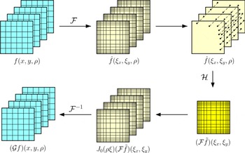
Our numerical scheme for computing ${\mathcal{G}}f$ is summarised in figure 2. In this figure, we omitted for simplicity the time dependence of all the quantities, since the computation of ${\mathcal{G}}f$ is done at fixed $t$ . The parallel planes represent the spatial (in blue) or Fourier (in yellow) grids for different values of $\unicode[STIX]{x1D70C}$ . The Hankel step ${\mathcal{H}}$ collapses the $N_{\unicode[STIX]{x1D70C}}$ planes into a single plane, which contains the data corresponding to the Fourier transform of $\tilde{f}$ . Multiplying ${\mathcal{F}}\tilde{f}$ by $\text{J}_{0}(\unicode[STIX]{x1D70C}\unicode[STIX]{x1D709})$ , we recreate $N_{\unicode[STIX]{x1D70C}}$ panels on which we apply the inverse Fourier transform ${\mathcal{F}}^{-1}$ to obtain the desired ${\mathcal{G}}f$ .

Figure 2.

Graphical representation of the successive steps involved in the numerical evaluation of ${\mathcal{G}}f$ . The lines in each coloured plane correspond to lines of constant $x$ and constant $y$ and we note the equispaced grid for the spatial variables and the Chebyshev grid in Fourier space. The successive planes correspond to different values of the variable $\unicode[STIX]{x1D70C}$ . Since the computation of ${\mathcal{G}}f$ is done at a fixed time $t$ , we omitted the time dependence in all the formulae in this figure.

4.1 Accuracy of our scheme

For the sake of definiteness, in our experiments we put $A=B=15$ . Consistent with what we have already explained, we choose the following fixed interval sizes for the various grids involved in our numerical scheme.

We define the sampling rate of a particular grid to be the number of grid points per unit length. For a particular experiment, the sampling rates for the real space grid, Fourier space grid and gyroradius grid are denoted, respectively, $L_{N}$ , $L_{\hat{N}}$ and $L_{N_{\unicode[STIX]{x1D70C}}}$ . In the language of the previous sections, it follows that $L_{N}=N/a$ , $L_{\hat{N}}=\hat{N}/\hat{a}$ and $L_{N_{\unicode[STIX]{x1D70C}}}=N_{\unicode[STIX]{x1D70C}}/\overline{\unicode[STIX]{x1D70C}}$ .

Let ${\mathcal{G}}f^{\text{ex}}(x,y,\unicode[STIX]{x1D70C})$ denote the exact function in (4.2) and let ${\mathcal{G}}f^{\text{num}}(x,y,\unicode[STIX]{x1D70C})$ denote the numerical approximation to ${\mathcal{G}}f^{\text{ex}}$ obtained by applying our numerical scheme for gyroaveraging to the function $\tilde{f}$ in (4.1). For our purposes, we are concerned with the relative maximum error $\unicode[STIX]{x1D716}_{\text{abs}}$ , defined as

where $(x_{i},y_{j},\unicode[STIX]{x1D70C}_{k})$ is a grid point in $[-3,3]^{2}\times [0,1.55]$ .

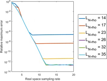
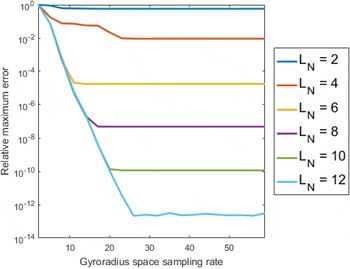
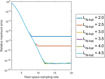
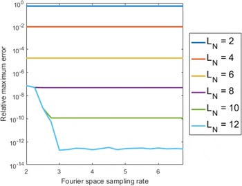
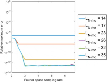
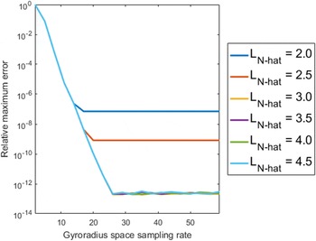
We have calculated and plotted (on a log scale) $\unicode[STIX]{x1D716}_{\text{abs}}$ for a wide range of sampling rates on each grid. In figures 3–8, each pair of side-by-side figures shows $\unicode[STIX]{x1D716}_{\text{abs}}$ for a fixed sampling rate of a particular grid. In figures 3–4 we see $\unicode[STIX]{x1D716}_{\text{abs}}$ for a fixed sampling rate on the real space grid, in figures 5–6 we see $\unicode[STIX]{x1D716}_{\text{abs}}$ for a fixed sampling rate on the Fourier space grid and in figures 7–8 we see $\unicode[STIX]{x1D716}_{\text{abs}}$ for a fixed sampling rate on the gyroradius grid. The fixed sampling rates in each case are those explained and suggested previously. The figures clearly show that with the combined suggested choices $L_{N}=12$ , $L_{\hat{N}}=4.5$ and $L_{N_{\unicode[STIX]{x1D70C}}}=35$ , the error $\unicode[STIX]{x1D716}_{\text{abs}}$ is of the order of approximately $10^{-13}$ . Generally, the error decreases exponentially as we increase all three sampling rates uniformly, which is a hallmark of numerical schemes based on spectral methods.

Figure 3.

Plot of $\unicode[STIX]{x1D716}_{\text{abs}}$ as a function of $L_{\hat{N}}$ and selected values of $L_{N_{\unicode[STIX]{x1D70C}}}$ , for the fixed real sampling rate $L_{N}=12$ .

Figure 4.

Plot of $\unicode[STIX]{x1D716}_{\text{abs}}$ as a function of $L_{N_{\unicode[STIX]{x1D70C}}}$ and selected values of $L_{\hat{N}}$ , for the fixed real sampling rate $L_{N}=12$ .

Figure 5.

Plot of $\unicode[STIX]{x1D716}_{\text{abs}}$ as a function of $L_{N}$ and selected values of $L_{N_{\unicode[STIX]{x1D70C}}}$ , for the fixed Fourier sampling rate $L_{\hat{N}}=4.5$ .

Figure 6.

Plot of $\unicode[STIX]{x1D716}_{\text{abs}}$ as a function of $L_{N_{\unicode[STIX]{x1D70C}}}$ and selected values of $L_{N}$ , for the fixed Fourier sampling rate $L_{\hat{N}}=4.5$ .

Figure 7.

Plot of $\unicode[STIX]{x1D716}_{\text{abs}}$ as a function of $L_{N}$ and selected values of $L_{\hat{N}}$ , for the fixed gyroradius sampling rate $L_{N_{\unicode[STIX]{x1D70C}}}=35$ .

Figure 8.

Plot of $\unicode[STIX]{x1D716}_{\text{abs}}$ as a function of $L_{\hat{N}}$ and selected values of $L_{N}$ , for the fixed gyroradius sampling rate $L_{N_{\unicode[STIX]{x1D70C}}}=35$ .

4.2 Run-time results

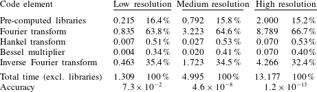
We are also interested in the CPU run time of our code, in particular, the relative run times of the various elements involved (i.e. forward Fourier transform, Hankel transform, Bessel function multiplier and inverse Fourier transform). For this purpose, we have run multiple simulations for selected sampling rates for computing the gyroaverage of the function in (4.1), and we have collected our results in table 1. For each resolution, the left-hand column corresponds to the time elapsed in seconds and the right-hand column to the time elapsed as a percentage of the total time.

We have separated the run-time data for the specific code elements from the run-time data for computing the various libraries in our code (e.g. Hankel transform weights, Chebyshev grid in Fourier space, etc.). The intended purpose of our gyroaveraging code is its use in solving the gyrokinetic-Poisson equations. Thus the gyroaveraging code is run at each time step, and so the pre-computed libraries need be computed only once and not at each time step. Thus when analysing the relative time of the code elements, it is not appropriate to include the time taken to build those libraries. Hence the percentage times reported in table 1 are percentages relative to the total time elapsed excluding the time taken to build the libraries.

Although we show the absolute run-time data, given in seconds, for completeness, their importance and relevance are limited. Indeed, we have implemented our scheme in MATLAB, which is an interpreted language and therefore slower than compiled languages such as Fortran and C for the algorithms we rely on, often by an order of magnitude. Furthermore, our results were obtained by running our code on a single core, and we have not yet explored methods for accelerating our schemes through parallelisation.

In contrast, the conclusions we can make from the relative elapsed times of each code element are instructive and as follows. First, we see that the relative elapsed times are approximately the same for all resolutions. Second, the Hankel transform and Bessel function multiplication together take less than 1 % of the total time. This observation is consistent with the fact observed in § 3 that the complexity of the Hankel transform (i.e. $O(N_{\unicode[STIX]{x1D70C}}\hat{P})$ ) is less than the complexity of the Fourier transforms (i.e. $O(N_{\unicode[STIX]{x1D70C}}(P+\hat{P})\log (P+\hat{P}))$ ). The elapsed time is dominated by the time taken by the Fourier transform and the inverse Fourier transform, with the former taking about twice as long as the latter. This difference in time is due to the use of the FST in the forward transform but not in the inverse transform. Finally, we simply note that the computation of the libraries takes about 16 % as long as one iteration of the gyroaveraging code.

Table 1.

For each set of resolutions and for each code element, the CPU run time is reported in two ways: the time elapsed in seconds and the time elapsed as a percentage of the total time (excluding the time required to pre-compute the necessary libraries). The specific sampling rates used for each resolution were $(L_{N},L_{\hat{N}},L_{N_{\unicode[STIX]{x1D70C}}})=(4,2.5,11)$ for ‘low resolution’, $(L_{N},L_{\hat{N}},L_{N_{\unicode[STIX]{x1D70C}}})=(8,3.5,23)$ for ‘medium resolution’ and $(L_{N},L_{\hat{N}},L_{N_{\unicode[STIX]{x1D70C}}})=(12,4.5,35)$ for ‘high resolution’. The ‘high resolution’ sampling rates are the sampling rates we have suggested in § 3. These data were obtained by averaging the results of 1000 separate simulations of our code in Matlab on a home desktop computer operating on an Intel i7-6700k processor at 4.0 GHz.