1 Introduction
The effects of surface roughness on laminar boundary layers is a long-lasting problem and particularly driven by the increasing demand for economical and sustainable flight. Early observations on isolated, three-dimensional (3-D) roughness elements are summarized in § 1.1 to provide an overview of known experimental and numerical observations. Some of the physical mechanisms, however, are not fully understood, and as a consequence, the definition of the ‘critical’ roughness Reynolds number has been rather ambiguous up to now. Global linear stability theory is a relatively new and promising tool to predict laminar–turbulent transition of certain flows unambiguously. The objective of this experimental investigation is to provide a comparison to recent theoretical advances described in § 1.2.
1.1 Roughness-induced instability
One of the first investigations of 3-D isolated roughness elements was done by Gregory & Walker (Reference Gregory and Walker1956), who visualized a steady horseshoe vortex that wraps around the front side of the roughness and then travels downstream as a pair of counter-rotating, streamwise vortices. They also observed a pair of vortices in the aft recirculation zone which develops into periodic vortex shedding with the shape of a hairpin if the roughness is high enough. This observation was also made by Mochizuki (Reference Mochizuki1961a ,Reference Mochizuki b ) and linked to the rapid laminar–turbulent transition in the roughness wake. Later, hairpin vortices were studied in detail by Acarlar & Smith (Reference Acarlar and Smith1987) who found strong similarity to the turbulence production process in the near-wall transitional boundary layer. Klebanoff, Tidstrom & Sargent (Reference Klebanoff, Tidstrom and Sargent1962) attributed this observation to a Kelvin–Helmholtz (KH) type of instability, which was later substantiated by Klebanoff, Cleveland & Tidstrom (Reference Klebanoff, Cleveland and Tidstrom1992) and more recently by Ergin & White (Reference Ergin and White2006).
Another characteristic feature of 3-D roughness elements is streamwise elongated, steady streaks of alternating high- and low-speed fluid. Such streaks arise from an exchange of momentum of the near- and far-wall boundary layer through streamwise vorticity and can be depicted as a scar being ripped into the boundary layer (Andersson et al. Reference Andersson, Brandt, Bottaro and Henningson2001). The mechanism has been known since early visualizations by Mochizuki (Reference Mochizuki1961a ) and was later denoted the ‘lift-up effect’ by Landahl (Reference Landahl1990). From a theoretical point of view, boundary layer streaks can be linked to transient growth (Reshotko Reference Reshotko2001), which relies on the non-orthogonality of eigenmodes resulting in short-term growth in contrast to the classic modal growth of Tollmien–Schlichting (TS) waves. Andersson, Berggren & Henningson (Reference Andersson, Berggren and Henningson2005) found that the so-called ‘optimal’ disturbances, leading to the maximum transient growth, are steady, streamwise vortices for a flat-plate boundary layer. If the amplitude of the resulting optimal streaks grows larger than 26 % of the free-stream velocity, secondary instabilities can set in (Andersson et al. Reference Andersson, Brandt, Bottaro and Henningson2001). However, White (Reference White2002) found that neither wall-normal disturbance profiles nor the streamwise stations of maximum disturbance growth match between roughness streaks and transient growth theory. Denissen & White (Reference Denissen and White2013) analysed this problem theoretically and with direct numerical simulation (DNS) and confirmed that optimal growth is more present in the mid-wake where exponential growth may have already caused transition. The DNS of Rizzetta & Visbal (Reference Rizzetta and Visbal2007) confirmed earlier findings of strong hairpin vortex shedding downstream of the roughness. Bi-local, or ‘biglobal’ (Theofilis Reference Theofilis2011) stability computations of streamwise planes in the roughness wake have been done by Denissen & White (Reference Denissen and White2013) and Shin, Rist & Krämer (Reference Shin, Rist and Krämer2015). In the work by Shin et al. (Reference Shin, Rist and Krämer2015) the two unstable 2-D modes were either of sinuous or varicose shape, whereas the varicose mode could be associated with hairpin vortex shedding and was thus much more distinct in the water channel experiment than the sinuous mode. Theoretical predictions by bi-local stability theory are promising, but a major shortcoming is the restriction to parallel flows.
Besides understanding the flow topology, many early workers were particularly motivated to identify criteria for laminar–turbulent transition. As already suggested by Schiller (Reference Schiller1932) and advanced by Klanfer & Owen (Reference Klanfer and Owen1953), the roughness Reynolds number
 $Re_{kk}=u_{k}k/\unicode[STIX]{x1D708}$
, where
 $k$
is the roughness height,
 $u_{k}$
the streamwise velocity at the tip of the roughness of the undisturbed boundary layer and
 $\unicode[STIX]{x1D708}$
the kinematic viscosity, is deemed best as a measure for roughness-induced transition. Sometimes the control parameter is also the Reynolds number
 $Re_{k}=U_{e}k/\unicode[STIX]{x1D708}$
based on the boundary layer edge velocity
 $U_{e}$
, but the majority of the literature prefers to use
 $Re_{kk}$
. Based on this parameter, Klanfer & Owen (Reference Klanfer and Owen1953) reanalysed the data of Gregory & Walker (Reference Gregory and Walker1956) and found transition occurring at
 $Re_{kk,tr}=440$
for conical roughness, and similarly, Tani (Reference Tani1961) found
 $500<Re_{kk,tr}<800$
for hemispherical roughness elements with the data of Klebanoff, Schubauer & Tidstrom (Reference Klebanoff, Schubauer and Tidstrom1955). In another study, Tani et al. (Reference Tani, Komoda, Komatsu and Iuchi1962) detected transition in a range of
 $600<Re_{kk,tr}<1000$
. In their attempt to organize early data, von Doenhoff & Braslow (Reference von Doenhoff and Braslow1961) found that
 $Re_{kk,tr}$
is lower for increasing aspect ratios
 $\unicode[STIX]{x1D702}=d/k$
, where
 $d$
is the roughness diameter. They presented a famous transition diagram which is still used in many engineering applications to date. Nevertheless, the spread between published data remains large, most authors accounting differences in roughness shape and experimental detection methods for the observed deviations, but also pressure gradients and free-stream turbulence (FST) (Klebanoff et al.
Reference Klebanoff, Cleveland and Tidstrom1992). In a more recent investigation at the low turbulence wind tunnel at KTH Sweden, Fransson et al. (Reference Fransson, Brandt, Talamelli and Cossu2005) reported a stabilizing effect of cylindrical roughness arrays with respect to TS instability. The upper limit of their technique was determined to be
 $Re_{kk,tr}=422$
with rapid transition when this value was exceeded. Although the published data from the last and present century are extensive and helpful for many purposes, they neither give an unambiguous transition criterion nor explain basic processes that lead to roughness-induced laminar–turbulent transition.
1.2 Global stability theory
Three-dimensional global, or ‘triglobal’ (Theofilis Reference Theofilis2011) linear stability theory (LST) provides global instability modes by solving the linearized Navier–Stokes equations as an eigenvalue problem with a disturbance ansatz in all three spatial directions. This is an advancement from bi-local stability theory, which is restricted to the parallel-flow assumption. Therefore, 3-D global LST is particularly beneficial for highly non-parallel flows such as roughness wakes. One drawback of 3-D global LST is the enormous memory requirement, which often means that numerical techniques such as Krylov subspaces must be used for computability (Bagheri et al.
Reference Bagheri, Akervik, Brandt and Henningson2009). The changeover from a globally stable to unstable system typically occurs when increasing a control parameter such as
 $Re_{kk}$
beyond a certain threshold. Mathematically speaking, this event is a supercritical Hopf bifurcation from a stable fixed point to a limit cycle oscillation. In a physical system the latter state reveals itself as self-sustained, intrinsic system oscillations, independent of external noise. Such a system is often called an oscillator or wavemaker and should be distinguished from an amplifier which only amplifies external noise. Descriptive introductions to nonlinear dynamics and linear stability theory can be found in the book of Manneville (Reference Manneville2004) and the review article by Theofilis (Reference Theofilis2011), respectively.
Closely related classifications are local absolute and convective instabilities. Whereas local absolute instabilities grow temporally at a fixed location, convective instabilities can only grow if they travel in the downstream direction. In this sense, local absolute and global instabilities are similar except for their different spatial extent. Huerre & Monkewitz (Reference Huerre and Monkewitz1990) showed that 3-D global instability can ignite within a reasonably large streamwise extent of local absolute instability and Chomaz, Huerre & Redekopp (Reference Chomaz, Huerre and Redekopp1991) and Monkewitz, Huerre & Chomaz (Reference Monkewitz, Huerre and Chomaz1993) concluded that within the linear and weakly non-parallel approximation, local absolute instability is in general a necessary condition for the existence of 3-D global instability. The restriction of linearity and weak non-parallelism was later abolished for more general conditions as described in the review article by Chomaz (Reference Chomaz2005).
Three-dimensional global stability analyses on roughness elements have been done by Loiseau et al. (Reference Loiseau, Cherubini, Robinet and Leriche2014) who found that the first unstable global mode is varicose (symmetric) for large aspect ratios and sinuous (antisymmetric) for small aspect ratios. Apparently the two modes compete against each other as in the observations by Asai, Minagawa & Nishioka (Reference Asai, Minagawa and Nishioka2002) for pieces of screens inside the boundary layer. However, to our knowledge, there has been no physical experiment on this observation for roughness elements yet. Further, the practical significance of global modes in roughness-induced transition is still unclear, particularly due to the convective nature of the flow (Asai et al. Reference Asai, Minagawa and Nishioka2002; Brandt et al. Reference Brandt, Cossu, Chomaz and Huerre2003) and transiently growing perturbations (Cherubini et al. Reference Cherubini, De Tullio, De Palma and Pascazio2013). As shown by Chomaz (Reference Chomaz2005), transient growth can be considered as a convective instability from a local point of view and as non-normality of the evolution operator from a global point of view. In this work, instead of immersing ourselves in a theoretical analysis, we aim at directly clarifying the role of 3-D global LST and its critical Reynolds number in a physical experiment.
In theory, the significance of the critical Reynolds number is clear: when the growth rate of a mode becomes positive for the first time, the system is unstable. Experimentally, it requires innovative strategies to detect a globally or absolutely unstable flow unambiguously and therefore some successful examples are summarized here. One prominent example is the vortex shedding behind 2-D cylinders. Sreenivasan, Strykowski & Olinger (Reference Sreenivasan, Strykowski, Olinger and Ghia1987) determined the constants of the Landau equation for this flow in the vicinity of the critical Reynolds number and thus showed experimentally that the vortex shedding is due to a Hopf bifurcation as typically encountered when global modes become unstable. For the problem of rotating disc flows, Lingwood (Reference Lingwood1996) detected absolute instability by inducing a perturbation in the form of a wavepacket that spreads in time as it travels outside towards higher Reynolds numbers: the front velocity of the wavepacket remains constant whereas the rear velocity asymptotically approaches zero. Inspired by this work, a similar procedure will be applied here. For the plane sheet flow de Luca (Reference de Luca1999) observed the angle at which disturbances spread from a small wire spanned perpendicular to the plane sheet flow. His criterion for absolute instability was when the disturbance angle approached
 $90^{\circ }$
. A changeover from convective to absolute instability has also been found experimentally in a rotating Hagen–Poiseuille flow by observing the inlet region of the pipe in Shrestha et al. (Reference Shrestha, Parras, Del Pino and Sanmiguel-Rojas2012) and later more quantitatively by measuring wavepacket fronts travelling upstream and downstream during pipe spin-down (Miranda-Barea et al.
Reference Miranda-Barea, Fabrellas-Garcia, Parras and del Pino2016). Gondret et al. (Reference Gondret, Ern, Meignin and Rabaud1999) found global instability in a Hele-Shaw cell; however, their technique can also be hardly applied here. In the case of 3-D roughness in a boundary layer, Kurz & Kloker (Reference Kurz and Kloker2016) showed with DNS that after exposing a roughness of a certain height to controlled disturbances, turbulence appears behind the roughness and even remains after switching off the disturbance source. This indicates the existence of a self-sustained mode; however, this study has been done for a roughness bump in cross-flow and for artificial base flows with selective frequency damping. What has been missing to date is a physical experiment detecting global instability in a 3-D isolated roughness case. Preliminary work has been done by Puckert & Rist (Reference Puckert and Rist2018), where time traces and spectral data strongly support the 3-D global instability from theory for one case. Motivated by this observation, a more extensive study is provided here to extend the predominant belief in the literature that roughness instabilities are of a convective, not absolute nature. Earlier results by Puckert & Rist (Reference Puckert, Rist, Dillmann, Heller, Krämer, Radespiel and Wagner2016) reveal good agreement of the frequencies of the first unstable global mode and vortex shedding in the experiment. Also, the mode shape for larger aspect ratios seems to be in good agreement with the physical observation. However, vortex shedding typically occurs earlier than predicted by theory. Bucci et al. (Reference Bucci, Puckert, Andriano, Loiseau, Cherubini, Robinet and Rist2018) explained this phenomenon by quasi-resonance of a global mode, meaning that background noise can be selectively amplified by the roughness at a frequency identical to the global mode. Pseudospectra analysis revealed that the effect of non-modal growth is rather small. The contradiction in the previous literature is that the roughness seems to act both as an amplifier and as an oscillator. This issue is still to be resolved and addressed in the present work. To be more specific we aim at the following main questions.
(i) Can the critical Reynolds numbers from global LST be confirmed experimentally?
(ii) When is the roughness an amplifier or wavemaker?
(iii) Can both varicose and sinuous modes be found in an experiment?
(iv) What is the physical relevance of global instability?
This paper is structured as follows. In § 2 the facility, experimental methods and procedures are explained, in § 3 a comparison between numerical base flow and experimental mean flow is provided and § 4 introduces a key problem on the transition Reynolds number versus the critical Reynolds number in the literature. This problem is resolved in § 5 with the present experimental data. The difference between amplifier and wavemaker in regard to roughness wakes is presented in § 6. Further, the difficult detection of the sinuous mode in experiments is resolved and also discussed in § 6.
2 Experimental methods
The experimental work of this investigation has been done in the laminar water channel (Laminarwasserkanal, LaWaKa) at the Institute of Aerodynamics and Gasdynamics (IAG), University of Stuttgart. It is a closed-loop facility with a
 $8\times 1.2\times 0.2\,\text{m}^{3}$
test section. Wiegand (Reference Wiegand1996) reported a low turbulence intensity of
 $0.05\,\%$
of the free-stream velocity in the frequency range
 $0.1{-}10~\text{Hz}$
at
 $0.145~\text{ms}^{-1}$
. At low velocities, low-frequency disturbances start to rise due to thermal stratification in the contraction and can be reduced by additional screens in front of the test section: see Puckert, Dieterle & Rist (Reference Puckert, Dieterle and Rist2017). The advantages of this water channel are the great boundary layer length and time scales compared to similar wind tunnels, which allows one to observe phenomena in greater detail both visually and quantitatively. As a drawback, the total measurement time can become huge and thus requires a high level of automation. To deal with this requirement, a 3-axes traverse system has been installed to traverse hot-film probes over the full extent of the test section. Good optical accessibility through the free surface and the glass walls further enable high-quality optical methods such as visualizations (Puckert et al.
Reference Puckert, Subasi, Rist and Gunes2015) and particle image velocimetry (PIV) (Lang, Rist & Wagner Reference Lang, Rist and Wagner2004). A permanently installed flat plate with elliptical leading edge creates a 2-D laminar boundary layer of Blasius-type with a shape factor
 $H_{12}$
deviation of only
 $\pm 3\,\%$
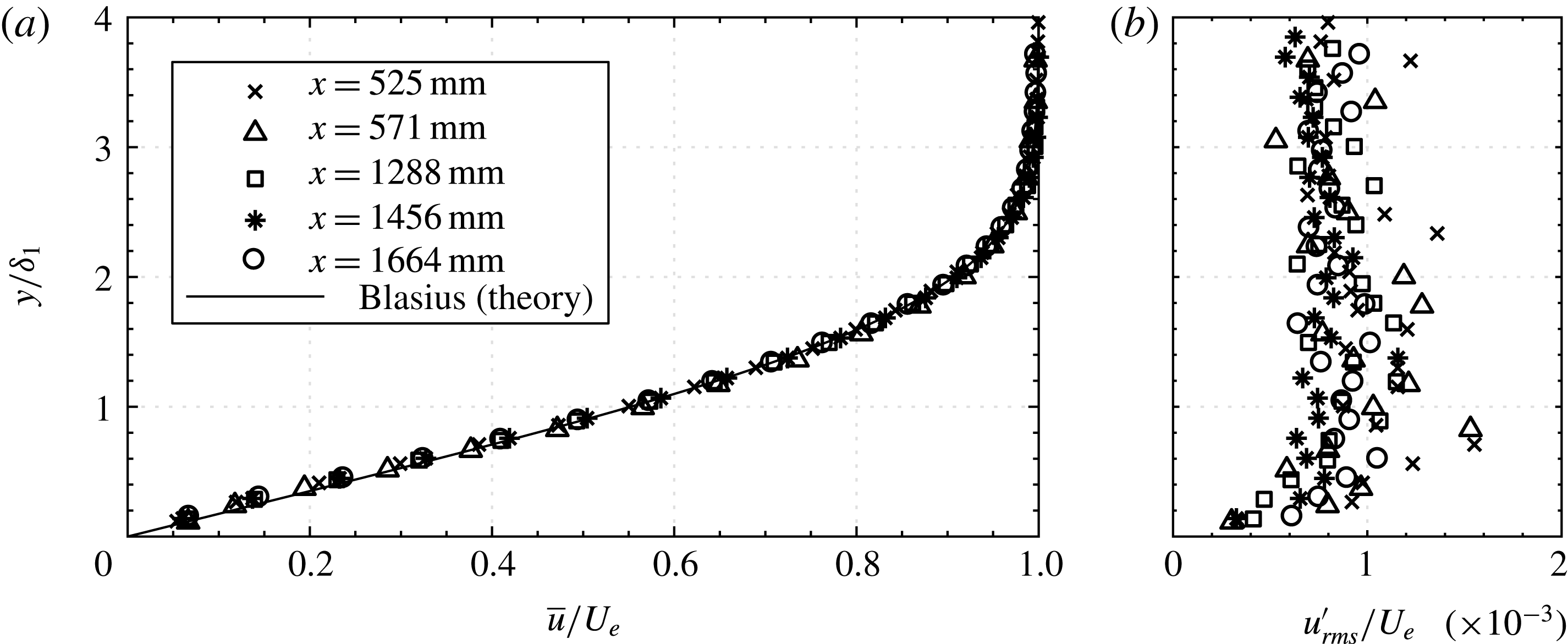
from theory (Wiegand Reference Wiegand1996). A wire mesh at the rear end of the flat plate provides a minor adverse pressure gradient for edge boundary layer suction between the flat plate and side walls. However, this pressure gradient is reduced by the growing boundary layer in the first part of the test section. Therefore, the Blasius equation can be used to describe the experimental velocity profile. This fact is illustrated by figure 1(a), where experimental profiles of different streamwise stations and free-stream velocities are compared to the theoretical profile. The measurement time was 60 s at each position and the experimental data show good agreement with the theoretical Blasius profile. Further, all velocity profiles in this figure are normalized by the theoretical displacement thickness
 $\unicode[STIX]{x1D6FF}_{1}$
based on the exact physical station, thus revealing if virtual origins are necessary or not. For the cases shown here and for the vast majority of experiments such corrections are not necessary; however, the flow quality was regularly monitored to ensure the Blasius assumption was valid. In rare cases virtual origins have been applied as described in Kachanov & Michalke (Reference Kachanov and Michalke1994), but even those are of the order of less than 2 % of the test section length. To enable a reproduction of our experiments in follow-up works, the wall-normal distribution of disturbance velocity root mean square (r.m.s.) is provided in figure 1(b). It can be seen that the disturbance intensity in the free stream is on average approximately
 $0.08\,\%$
for the cases considered here. The spread of measurements is due to the absence of external forcing and the influence of low-frequency disturbances. Spectral data of the turbulence intensity are provided for instance in Bucci et al. (Reference Bucci, Puckert, Andriano, Loiseau, Cherubini, Robinet and Rist2018).
Normalized wall distance
 $y/\unicode[STIX]{x1D6FF}_{1}$
versus (a) experimental mean velocity profiles
 $\bar{u}/U_{e}$
in comparison with theoretical Blasius profile and (b) disturbance velocity profiles
 $u_{rms}^{\prime }/U_{e}$
at various stations from the leading edge.

The roughness elements in this investigation are isolated cylinders with height
 $k$
, diameter
 $d$
and aspect ratio
 $\unicode[STIX]{x1D702}=d/k$
. They are made of stainless steel or brass and remain at any station
 $x_{k}$
solely by their own weight. Except for
 $x_{k}$
, which is measured from the leading edge, the right-handed coordinate system
 $xyz$
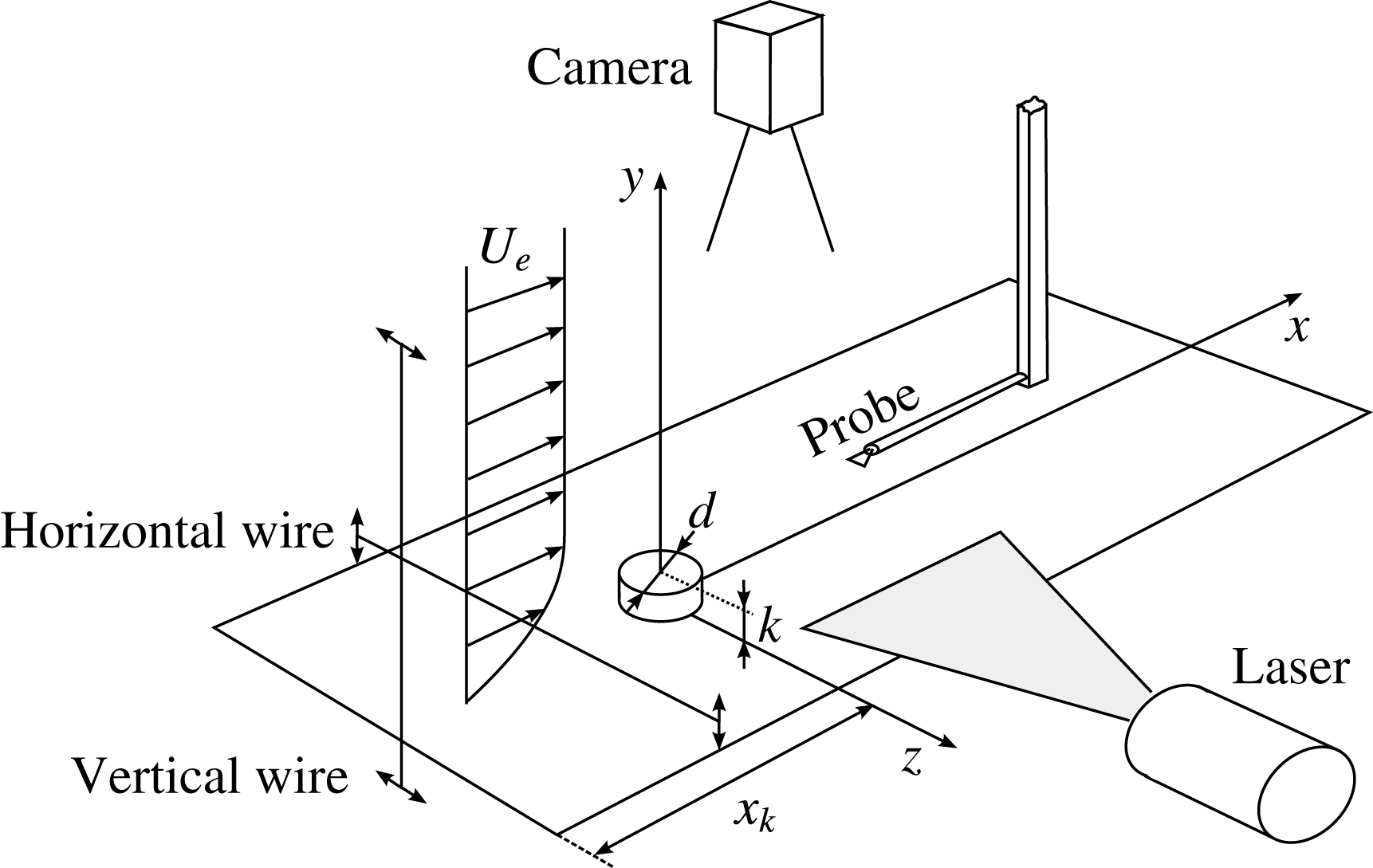
originates at the roughness element as shown in figure 2 and all length scales are normalized with respect to
 $k$
. The boundary layer edge velocity is denoted
 $U_{e}$
and the streamwise velocity at the roughness height is
 $u_{k}$
. In some experiments a classical horizontal vibrating wire is installed upstream of the roughness to force the flow with 2-D TS-like disturbances. The disturbance source is a 0.1 mm stainless steel wire which is moved sinusoidally up and down by two stepper motors connected to one eccentric wheel each. Another type of disturbance generator with spanwise mechanical excitation has been developed and improved according to the design of Shin et al. (Reference Shin, Rist and Krämer2015). Its vertical wire of diameter 1 mm is placed 1–2 cm upstream of the leading edge and is traversed sinusoidally by a linear actuator with an amplitude of 3 cm. In contrast to the horizontal wire, this construction does not introduce disturbances directly into the boundary layer but into the free stream where higher disturbance amplitudes are necessary. Data acquisition is done with a Dantec 55R15 hot-film probe, ‘Streamline’ bridge and an NI 16-bit A/D converter. The measurements can be triggered from one of the two disturbance generators to lock the measurement to the phase of the disturbance. King’s law is used to convert voltage into velocity signals which are decomposed into mean (
 $\bar{u}$
) and fluctuating component (
 $u^{\prime }$
). Digital filtering is applied between 0.1 and 10 Hz, and physical frequencies
 $f$
(Hz) are presented as circular frequencies
 $\unicode[STIX]{x1D714}=2\unicode[STIX]{x03C0}fkU_{e}^{-1}$
when deemed advantageous for a comparison to theory. The particle image velocimetry (PIV) system comprises a Q-switched dual-pulse Nd:YAG laser (Quantel Brilliant Twin W) with a wavelength of 532 nm, an external sequencer and a PCO Sensicam for image acquisition. Seeding is done with
 $4.2~\unicode[STIX]{x03BC}\text{m}$
polyamide particles.
Sketch of the experimental set-up.

3 Base flow comparison
Three-dimensional global linear stability analysis solves the linearized Navier–Stokes equations as an eigenvalue problem pertinent to a base flow of the particular flow field (Taira et al.
Reference Taira, Brunton, Dawson, Rowley, Colonius, McKeon, Schmidt, Gordeyev, Theofilis and Ukeiley2017). Often, the computation of a steady numerical base flow requires techniques such as selective frequency damping (SFD) to artificially settle the flow towards a steady equilibrium as described in Åkervik et al. (Reference Åkervik, Brandt, Henningson, Hœpffner, Marxen and Schlatter2006). This can be done by an extension of the Navier–Stokes equations with an additional feedback term and is therefore difficult to compare with physical flows for which there is no such technique. Further, physical flows may always behave nonlinearly if Reynolds numbers are high enough, thus invalidating the assumptions of LST. In this section, a comparison is done between a numerical base flow with SFD provided by the authors of Loiseau et al. (Reference Loiseau, Cherubini, Robinet and Leriche2014) and our experimental mean flow for the Reynolds number
 $Re_{k}=550$
. In Loiseau et al. (Reference Loiseau, Cherubini, Robinet and Leriche2014), this case is called the ‘Fransson experiment’ according to the intermittency experiment by Fransson et al. (Reference Fransson, Brandt, Talamelli and Cossu2005), and this case is slightly subcritical with respect to global modes.
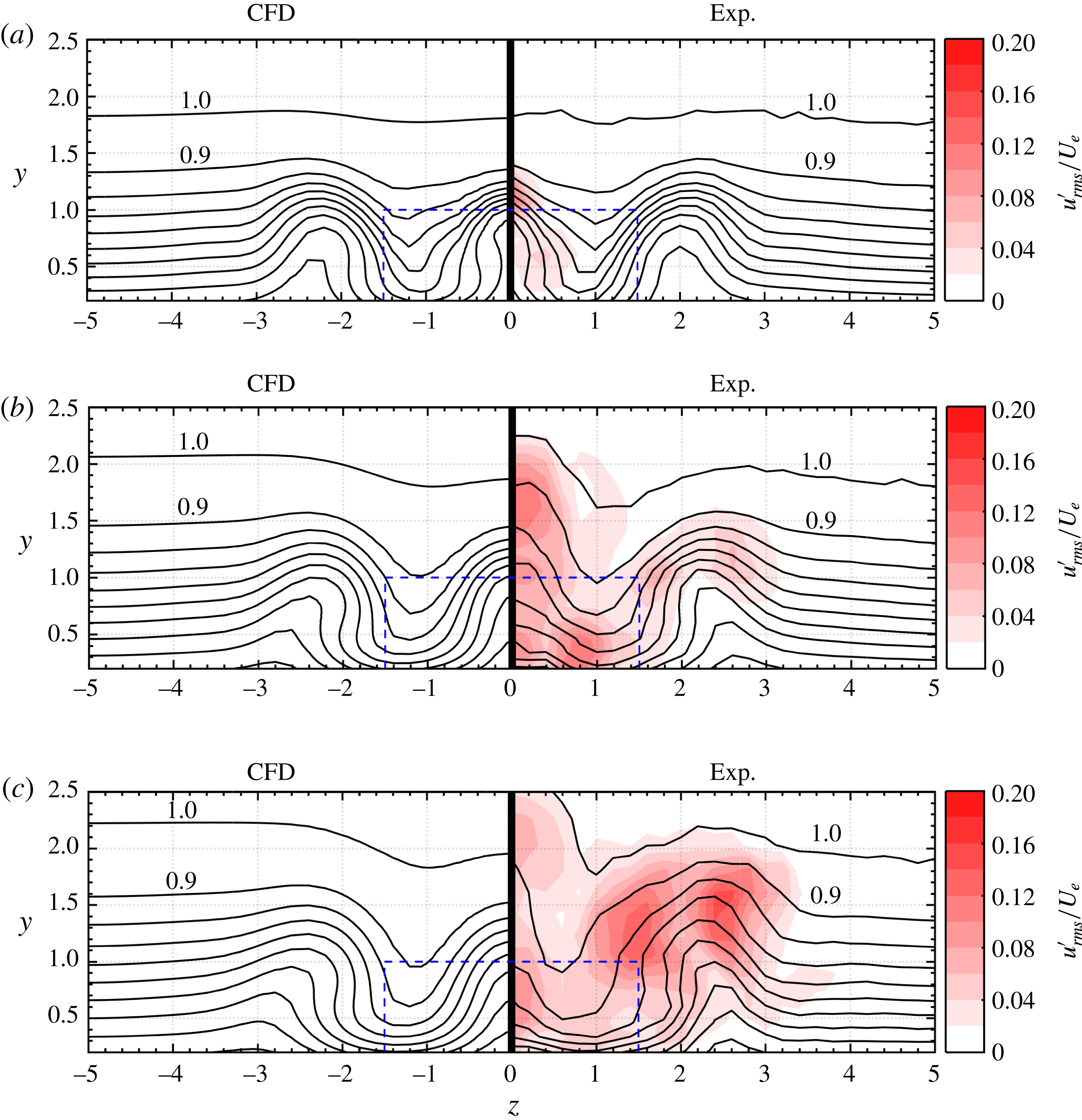
Comparison of numerical base flow kindly provided by Loiseau et al. (Reference Loiseau, Cherubini, Robinet and Leriche2014) on the left versus mean flow from experiments on the right at (a)
 $x=10$
, (b)
 $x=20$
and (c)
 $x=30$
. Contour levels show
 $\overline{u}/U_{e}$
from 0 to 1 in steps of 0.1.
 $Re_{k}=550$
,
 $\unicode[STIX]{x1D702}=3$
and
 $x_{k}=57.1$
(red online). Dashed lines (blue online) indicate roughness dimensions.

Figure 3 shows isolines of the normalized streamwise velocity from the numerical computation (Loiseau et al.
Reference Loiseau, Cherubini, Robinet and Leriche2014) on the left versus the normalized streamwise mean velocity from our experiments on the right at three streamwise slices
 $x=10$
, 20 and 30. Root mean squared (r.m.s.) velocity fluctuations are available from the experiment and are shown as red pseudocolours on the experimental side of the plots. To obtain these graphs, the hot-film has been traversed to
 $61\times 15$
equidistant points in
 $z$
and
 $y$
, respectively, each with 30 s measurement time. The first slice at
 $x=10$
demonstrates great qualitative agreement of both strength and location of velocity streaks resulting from streamwise vorticity induced by the roughness. High-speed streaks can be found where the isolines are closer to the wall, e.g. at approximately
 $z=\pm 1$
. Vice versa, low-speed streaks are regions of lifted isolines, e.g. at the spanwise centre and at approximately
 $z=\pm 2$
–3. In this slice, velocity disturbances are particularly located around the centre low-speed streak which can be attributed to inflection point instabilities of the KH type as explained by Klebanoff et al. (Reference Klebanoff, Cleveland and Tidstrom1992). In the slice
 $x=20$
, the disturbances become significantly stronger and even appear in regions of high shear around the outside low-speed streak at
 $z=2$
–3. In the slice at
 $x=30$
, the intensity of the disturbances in the centre slightly decreases and increases at
 $z=2$
–3 due to high spanwise shear. A quantitative analysis of the data has been done by calculating the mean relative deviation of the experimental flow from the numerical base flow. This yields 8 %, 10 % and 17 % deviation for
 $x=10$
, 20 and 30, respectively. In particular at
 $x=10$
there is good agreement of the velocity isolines whereas the deviations at
 $x=20$
and 30 are due to the absence of SFD in the experiment. Nonlinear interactions account for the distorted mean flow isolines and a comparison at these stations would thus be misleading. The agreement at
 $x=10$
, where nonlinearities are not yet strong enough, is satisfactory, considering the necessary but artificial selective frequency damping in numerical simulations and also the complexity of the experiment regarding facility-specific free-stream turbulence, measurement difficulties and tolerances of geometric and flow parameters. For lower Reynolds numbers the agreement would thus be as good as in figure 3(a). The question to be answered in the following is why there are obvious fluctuations in the experiment although theory predicts global stability!
4 Transition Reynolds number
The set-up of Fransson et al. (Reference Fransson, Brandt, Talamelli and Cossu2005) is reproduced at the LaWaKa to detect the transition Reynolds numbers and to compare with existing results. This case is particularly important because it has more recently been used by Loiseau et al. (Reference Loiseau, Cherubini, Robinet and Leriche2014) to compare to the critical Reynolds number obtained from a global stability analysis. The purpose of this section is to distinguish between global instability in theory and transition in a physical flow, which have been strongly linked in Loiseau et al. (Reference Loiseau, Cherubini, Robinet and Leriche2014). In contrast to these authors, we believe that this link is rather weak. To support our point of view, the transition detection method has to be explained first, followed by a brief verification study on the basis of the Fransson et al. (Reference Fransson, Brandt, Talamelli and Cossu2005) experiment and a comparison to theory. The results are then substantiated with a parameter study for different aspect ratios. The primary parameter in this section is the roughness Reynolds number
 $Re_{kk}$
to be in compliance with many other experimental works in the literature, and in particular with Fransson et al. (Reference Fransson, Brandt, Talamelli and Cossu2005) who used the same parameter but with different nomenclature.
4.1 Intermittency detection
Regarding the transition detection method, an intermittency function
 $\unicode[STIX]{x1D6FE}$
has been computed to detect turbulence as a function of
 $Re_{kk}$
. In contrast to methods using integral quantities like
 $c_{f}$
or
 $H_{12}$
, intermittency does not require
 $y$
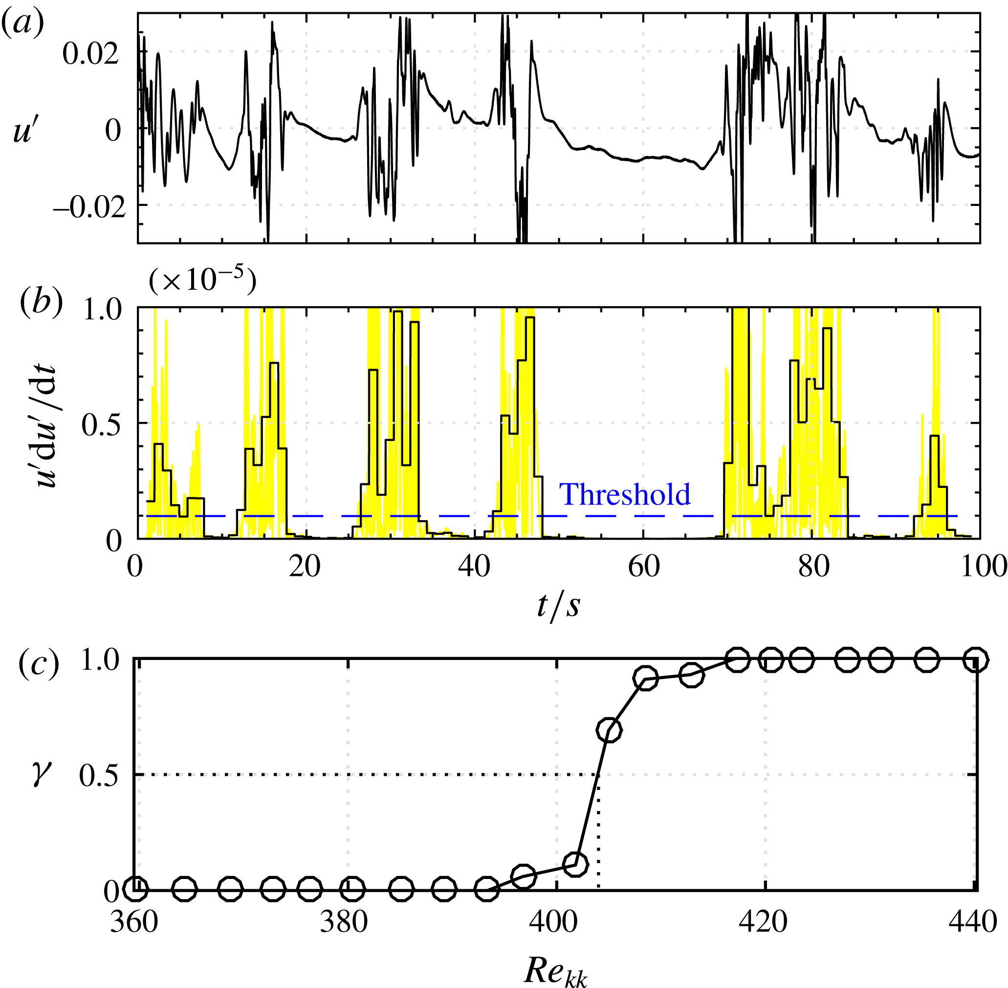
-profiles and is thus very suitable if measurement times are long. The computation follows the work of Zhang et al. (Reference Zhang, Xu, Pollard and Mi2013) and is demonstrated in figure 4. First, the signal
 $u^{\prime }$
in figure 4(a) is multiplied by its derivative
 $\text{d}u^{\prime }/\text{d}t$
to enhance the sensitivity to turbulence. The derivative is determined numerically based on wavelet transforms to smooth noisy experimental data (Luo, Bai & Shao Reference Luo, Bai and Shao2006). The detector function is then averaged into a criterion function every
 $1/100$
times of the signal length and compared to a threshold value which originates from a reference in laminar flow. The reference signal is multiplied by a constant factor in the range 1–10 to allow manual control of the method. These manual adjustments only become necessary when the set-up changes significantly. It has been found that the results do not change significantly as long as reasonable inputs are given. The intermittency function
 $\unicode[STIX]{x1D6FE}$
is the percentage of turbulence to the total signal length and can be estimated by summing up the parts of the signal where the criterion function is greater than the threshold value. An intermittency of 0 % or 100 % represents laminar or turbulent flow, respectively, and an intermittency of 50 % is the criterion to define the transition Reynolds number
 $Re_{kk,tr}$
. This value is considered as the ‘midpoint’ of transition (Halstead et al.
Reference Halstead, Wisler, Okiishi, Walker, Hodson and Shin1995; Stotz et al.
Reference Stotz, Wakelam, Guendogdu and Niehuis2014) and the same criterion has also been used by Fransson et al. (Reference Fransson, Brandt, Talamelli and Cossu2005). To detect this value for a specific configuration,
 $Re_{kk}$
was increased by increasing the free-stream velocity in steps of
 $7.5\times 10^{-4}~\text{m}~\text{s}^{-1}$
and evaluating the signal for each velocity at a fixed downstream station
 $(x,y,z)=(200,1,0)$
, similarly to Fransson et al. (Reference Fransson, Brandt, Talamelli and Cossu2005). Doing this gives illustrations as shown in figure 4(c) where the transition Reynolds number
 $Re_{kk,tr}$
is at
 $\unicode[STIX]{x1D6FE}=0.5$
. The results from this method are confirmed by dye streakline visualizations in a visual check. Further,
 $y$
-profiles have been measured to confirm the Blasius-flow assumption which is necessary to compute
 $Re_{kk}$
as a function of
 $u_{k}$
.
Intermittency computation: (a) streamwise disturbance signal
 $u^{\prime }$
, (b) detector function
 $u^{\prime }\,\text{d}u^{\prime }/\text{d}t$
(yellow online), criterion function (solid black line) and threshold value (dashed line, blue online) and (c) intermittency factor
 $\unicode[STIX]{x1D6FE}$
.

4.2 Transition in the Fransson et al. (Reference Fransson, Brandt, Talamelli and Cossu2005) experiment
The intermittency method was verified for the Fransson et al. (Reference Fransson, Brandt, Talamelli and Cossu2005) experiment with different roughness heights to see if
 $Re_{kk}$
is a general quantity which can be compared to the literature independent of dimensional quantities such as
 $k$
or
 $U_{e}$
. Three different roughness heights
 $k=3.5$
, 5 and 10 mm have been installed with constant
 $x_{k}=57.1$
and
 $\unicode[STIX]{x1D702}=3$
to match the set-up of Fransson et al. (Reference Fransson, Brandt, Talamelli and Cossu2005). Each experiment was done with both isolated elements and one periodic spanwise array of seven elements of the same type with spacing
 $\unicode[STIX]{x0394}z=10$
to investigate if arrays in numerical simulations with symmetry conditions or in experiments such as Fransson et al. (Reference Fransson, Brandt, Talamelli and Cossu2005) behave similarly. Moreover, the effect of hysteresis was investigated by determining the transition Reynolds number for both increasing and decreasing free-stream velocities.
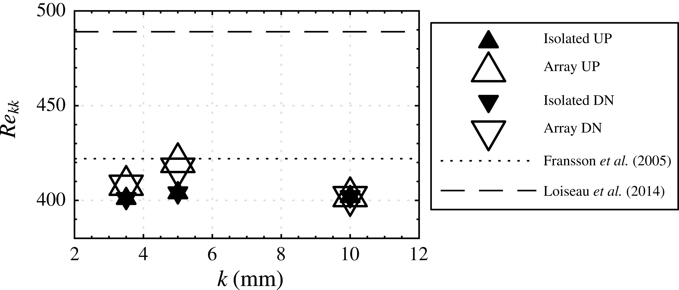
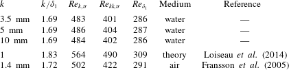
The results of this parameter study are summarized in figure 5 and table 1. Figure 5 shows transition Reynolds numbers of three different roughness heights, isolated elements versus arrays and increasing (‘UP’) versus decreasing (‘DN’) free-stream velocities. Figure 5 shows that none of these variations change the transition Reynolds number significantly. In particular the size of the roughness has no significant impact on transition, and for practical purposes
 $Re_{kk,tr}$
can therefore be considered as a general quantity if other parameters such as
 $k/\unicode[STIX]{x1D6FF}_{1}$
and
 $\unicode[STIX]{x1D702}$
are not changed. The differences between ‘UP’ versus ‘DN’ are negligible and are in agreement with Klebanoff et al. (Reference Klebanoff, Cleveland and Tidstrom1992) who investigated quasi-steady oscillating roughness heights and found no noteworthy hysteresis. Interestingly, the greatest difference seems to be in isolated versus array of roughness elements. Arrays are less prone to transition than isolated elements in four out of six cases. The spanwise periodicity of streaks seems slightly stabilizing, but this effect is within the given measurement accuracy and has not been investigated further. It can be concluded that the transition Reynolds number for the Fransson et al. (Reference Fransson, Brandt, Talamelli and Cossu2005) experiment in this work is
 $Re_{kk,tr}\approx 402$
with an accuracy of
 $\pm 5\,\%$
independent of the choice of
 $k$
,
 $U_{e}$
, isolated element or array. Fransson et al. (Reference Fransson, Brandt, Talamelli and Cossu2005) themselves found
 $Re_{kk,tr}=422$
, which is only
 $5\,\%$
higher than our result. The higher Reynolds number is probably due to the smaller turbulence intensity of the MTL wind tunnel at KTH Sweden and also within the given accuracy of the measurement. Unfortunately, the same cannot be said about the agreement with Loiseau et al. (Reference Loiseau, Cherubini, Robinet and Leriche2014), who found a theoretical critical Reynolds number of
 $Re_{k,c,t}=564$
, equivalent to
 $Re_{kk,c,t}=489$
. This discrepancy is graphically illustrated by the dashed line in figure 5 and is too high to be explained by measurement error. Apparently, transition does not coincide with global instability for this case. Note that Loiseau et al. (Reference Loiseau, Cherubini, Robinet and Leriche2014) reported good agreement with Fransson et al. (Reference Fransson, Brandt, Talamelli and Cossu2005), which may result from a comparison with
 $Re_{\unicode[STIX]{x1D6FF}_{1}}=U_{e}\unicode[STIX]{x1D6FF}_{1}/\unicode[STIX]{x1D708}$
instead of
 $Re_{kk}$
. As already explained in the introduction, we prefer the more established parameter
 $Re_{kk}$
for such a comparison because it is widely used in the literature and incorporates the effect of ‘blockage’ by the roughness more than any other boundary layer parameter.
Comparison of transition Reynolds numbers
 $Re_{kk,tr}$
for different roughness heights
 $k$
with results from the literature.

Verification study with different roughness heights (first three rows) and comparison with the literature (last two rows). In all cases roughness is isolated with
 $\unicode[STIX]{x1D702}=3$
and
 $x_{k}=57.1$
.

4.3 Parameter study
The same comparison has been repeated for the parameter study of Loiseau et al. (Reference Loiseau, Cherubini, Robinet and Leriche2014) with different aspect ratios
 $\unicode[STIX]{x1D702}=3$
, 2, 1 and 0.85. In contrast to the previous comparison, the streamwise station is now variable to obtain a constant height with respect to the displacement thickness
 $k/\unicode[STIX]{x1D6FF}_{1}=1.83$
. Experimentally, this requires us to reposition the roughness element many times manually. Such a procedure is practically difficult when experiments are long and not necessarily required if the boundary layer grows relatively slowly with
 $x$
. Similarly to the well-known parallel-flow assumption in theory, the experimental parameter study has been adapted in order for the experimental circumstances to retain the required level of automation. First, a fixed station
 $x_{k}$
has been determined at which theory predicts the Reynolds number to be critical. Then, only the free-stream velocity has been changed. The fixed station
 $x_{k}$
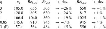
at which the roughness was placed in the experiment is provided in table 2. To distinguish
 $\unicode[STIX]{x1D702}=3$
of the parameter study from the Fransson et al. (Reference Fransson, Brandt, Talamelli and Cossu2005) experiment, the latter case is marked by ‘(F)’ in case of confusion.
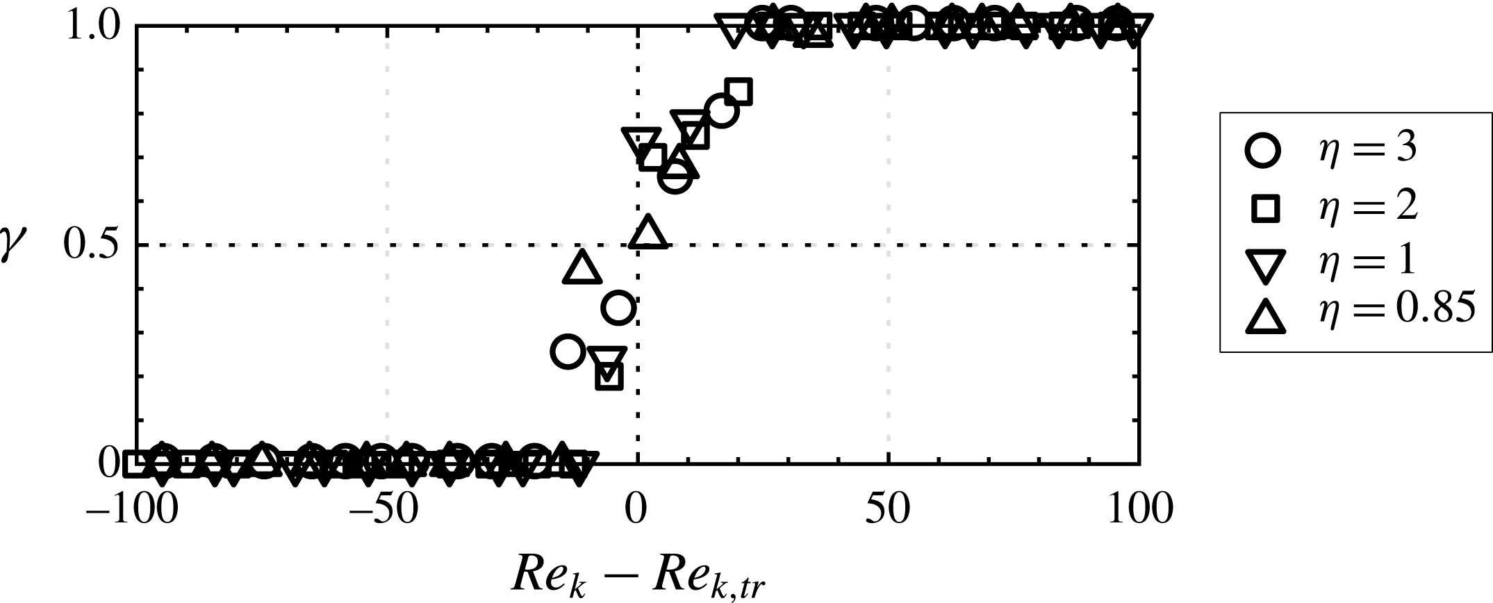
Comparing the transition Reynolds numbers determined as shown in figure 6 with the critical Reynolds numbers from theory confirms that there is again a discrepancy, as in the Fransson et al. (Reference Fransson, Brandt, Talamelli and Cossu2005) experiment. The relative deviation (dev.) between
 $Re_{k,tr}$
and
 $Re_{k,c,t}$
is given in table 2 and is computed with the formula dev.
 $=2\times (Re_{k,tr}-Re_{k,c,t})/(Re_{k,tr}+Re_{k,c,t})\times 100$
. Particularly for large aspect ratios, the relative error is large and reduces with smaller aspect ratio. A possible explanation for this phenomenon is related to the smaller receptivity to free-stream turbulence. More importantly, there is an obvious mismatch between theory and experiments for all cases in this parameter study despite the good agreement between the experimental mean flow and theoretical base flow (see § 3). Therefore, global instability may not be the decisive mechanism for transition at moderate Reynolds numbers and globally critical Reynolds numbers can hardly be compared to transition Reynolds numbers from experiments, contrary to what has been attempted by Loiseau et al. (Reference Loiseau, Cherubini, Robinet and Leriche2014). This attempt has also been done by the present authors in a visual attempt to find transition in Puckert et al. (Reference Puckert, Subasi, Rist and Gunes2015) but without the accuracy of a quantitative measurement technique. The relevance of global instability in roughness-induced transition must be different and the next section aims at shedding light on this apparent discrepancy.
Transitional and critical Reynolds numbers with deviations from theory (Loiseau et al. Reference Loiseau, Cherubini, Robinet and Leriche2014).

Intermittency of different aspect ratios
 $\unicode[STIX]{x1D702}$
.
 $Re_{k,tr}$
is provided in table 2. Probe position
 $(x,y,z)=(200,1,0)$
with 100 s measurement time for each Reynolds number.

5 Critical Reynolds number
The previous detection of transition Reynolds numbers has been done with the probe located in the far wake to measure turbulence without knowing which type of instability was responsible for laminar–turbulent breakdown. However, the critical Reynolds number is defined by the occurrence of the first (exponentially) growing disturbance, here with respect to global instability. It is therefore to be shown in this section if such a mechanism exists for all aspect ratios considered in this work. Measurements have been done closer to the roughness element in the range
 $0<x<40$
, where instability develops first. The probe is traversed within this range in equally spaced increments of
 $\unicode[STIX]{x0394}x=2$
at
 $y=1$
to measure the time traces of
 $u^{\prime }/U_{e}$
at different free-stream velocities (which is equivalent to changing the Reynolds number). The definition of the coordinate system origin at the roughness centre leads to different starting points for the probe, depending on aspect ratio; however, the spatial resolution is the same in all cases. The Reynolds number
 $Re_{k}$
is used instead of
 $Re_{kk}$
to enable a more direct comparison with Loiseau et al. (Reference Loiseau, Cherubini, Robinet and Leriche2014).
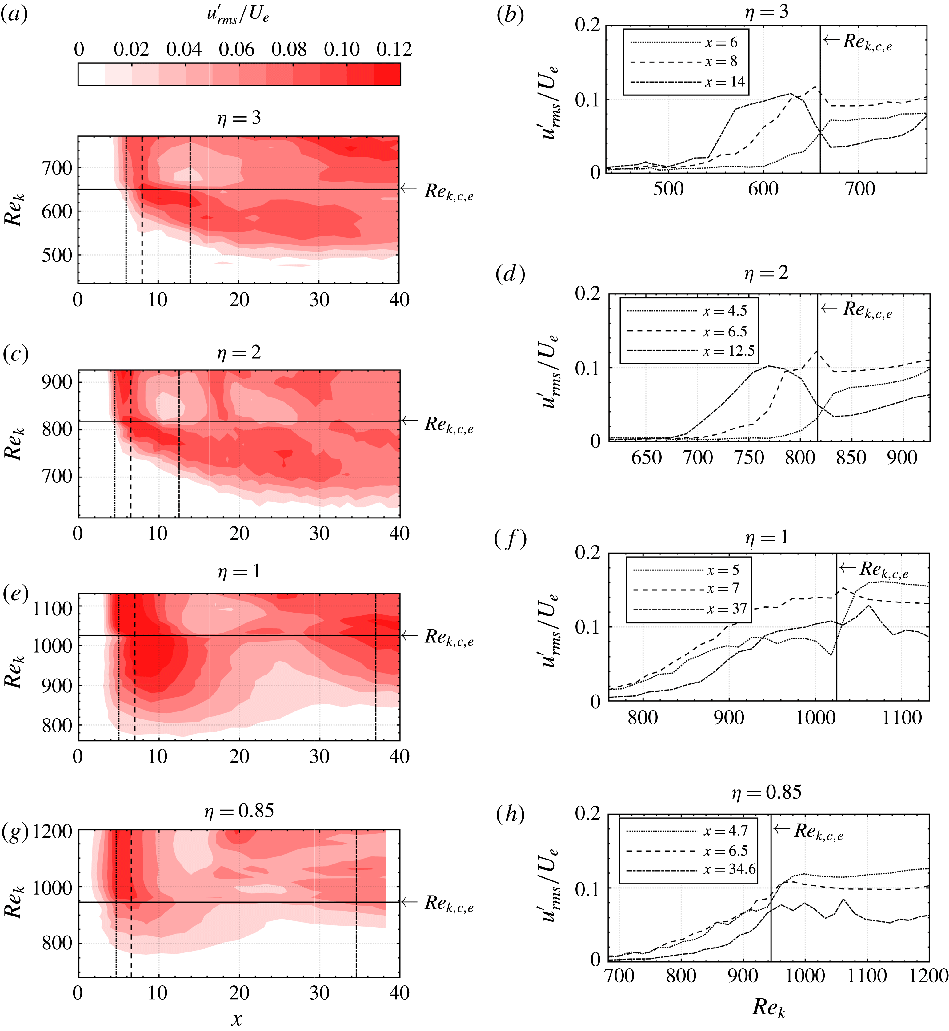
First, the r.m.s. streamwise velocity fluctuations are shown in figure 7(a,c,e,g) for different aspect ratios. In all plots it can be seen that the fluctuation r.m.s. grows with both increasing
 $x$
and
 $Re_{k}$
. When
 $Re_{k}$
is increased beyond the solid lines, the contours become more independent of
 $Re_{k}$
and remain at a constant streamwise station. These changes occur at one particular Reynolds number which will be denoted as the experimental critical Reynolds number
 $Re_{k,c,e}$
, analogous to the theoretical critical Reynolds number
 $Re_{k,c,t}$
. In contrast to
 $Re_{k,c,t}$
, which is the result of numerical–theoretical computations, the experimental critical Reynolds number
 $Re_{k,c,e}$
is a result of physical observation. It may be difficult to find
 $Re_{k,c,t}$
visually from these graphs, and other phenomena which are capable of detecting
 $Re_{k,c,e}$
have been summarized in Puckert & Rist (Reference Puckert and Rist2018). One such phenomenon has been developed to a robust detection method and is applied to the cases considered here. We will return to figure 7 and its right-hand side after a detection of
 $Re_{k,c,e}$
.
(a,c,e,g) Contour plots showing
 $u_{rms}^{\prime }/U_{e}$
for various
 $\unicode[STIX]{x1D702}$
(red online) and (b,d,f,h) line plots at particular streamwise stations indicated by the vertical lines in the left-hand side plots.

To determine the threshold
 $Re_{k,c,e}$
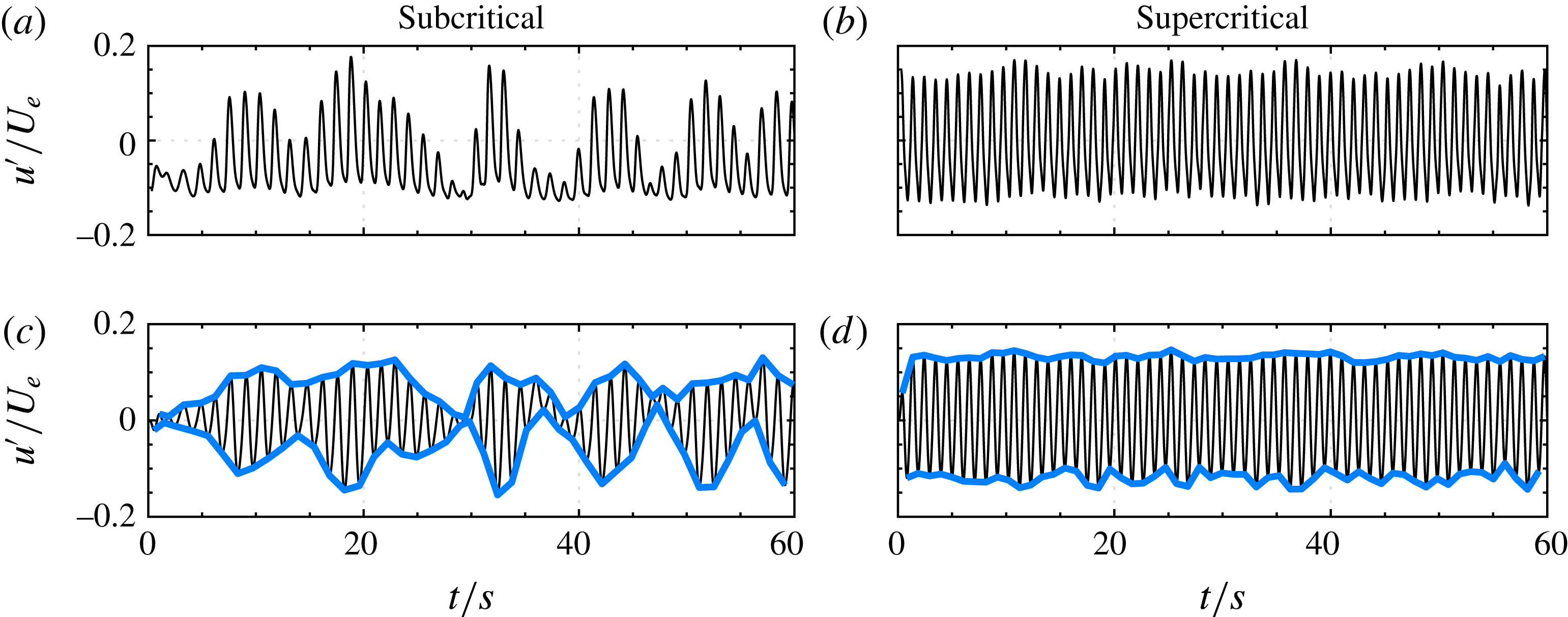
quantitatively, time-dependent fluctuation signals are evaluated. Figure 8(a,b) shows exemplary time traces for the case
 $\unicode[STIX]{x1D702}=3$
at
 $Re_{k}=600$
and 700, respectively. Interestingly, the signal at
 $Re_{k}=600$
fluctuates with somewhat randomly changing amplitudes, whereas the signal at
 $Re_{k}=700$
fluctuates with almost steady amplitude. This observation is exactly what can be expected from the difference between convective and global instability: the signal at
 $Re_{k}=600$
shows a typical shape of convective beatings from amplified unsteady noise that may later develop into intermittent turbulence, whereas the fluctuation amplitudes at
 $Re_{k}=700$
have grown to nonlinear saturation without depending on external noise. In other words, convective and global instability could be distinguished by the amount of envelope fluctuations, which allows for a simple detection of a threshold value. A procedure to determine the envelope functions requires smooth signals. Therefore, low-frequency oscillations, higher harmonics and noise are removed from the signal by bandpass filtering around the fundamental frequency
 $f_{0}$
, which can be determined by fast Fourier transformation. The filter setting was chosen to be 0.1–
 $1.7\times f_{0}$
, but a different choice does not alter the results significantly as long as higher harmonics are removed. Local extrema of the filtered signals can then be easily determined to form an envelope function: see figure 8(c,d). As a last step, the envelope r.m.s. is computed for both upper and lower envelopes and averaged to obtain one measure for the amplitude fluctuation. A high envelope r.m.s. is an indicator for convective instability and when crossing
 $Re_{k,c,e}$
, the envelope r.m.s. drops due to nonlinearly saturated signal amplitudes, most likely from a global instability.
Determination of critical Reynolds number based on envelope fluctuations: (a,b) time trace of
 $u^{\prime }/U_{e}$
and (c,d) filtered time trace with envelopes (blue solid lines).
 $Re_{k}=600$
for (a,c) and 700 for (b,d).

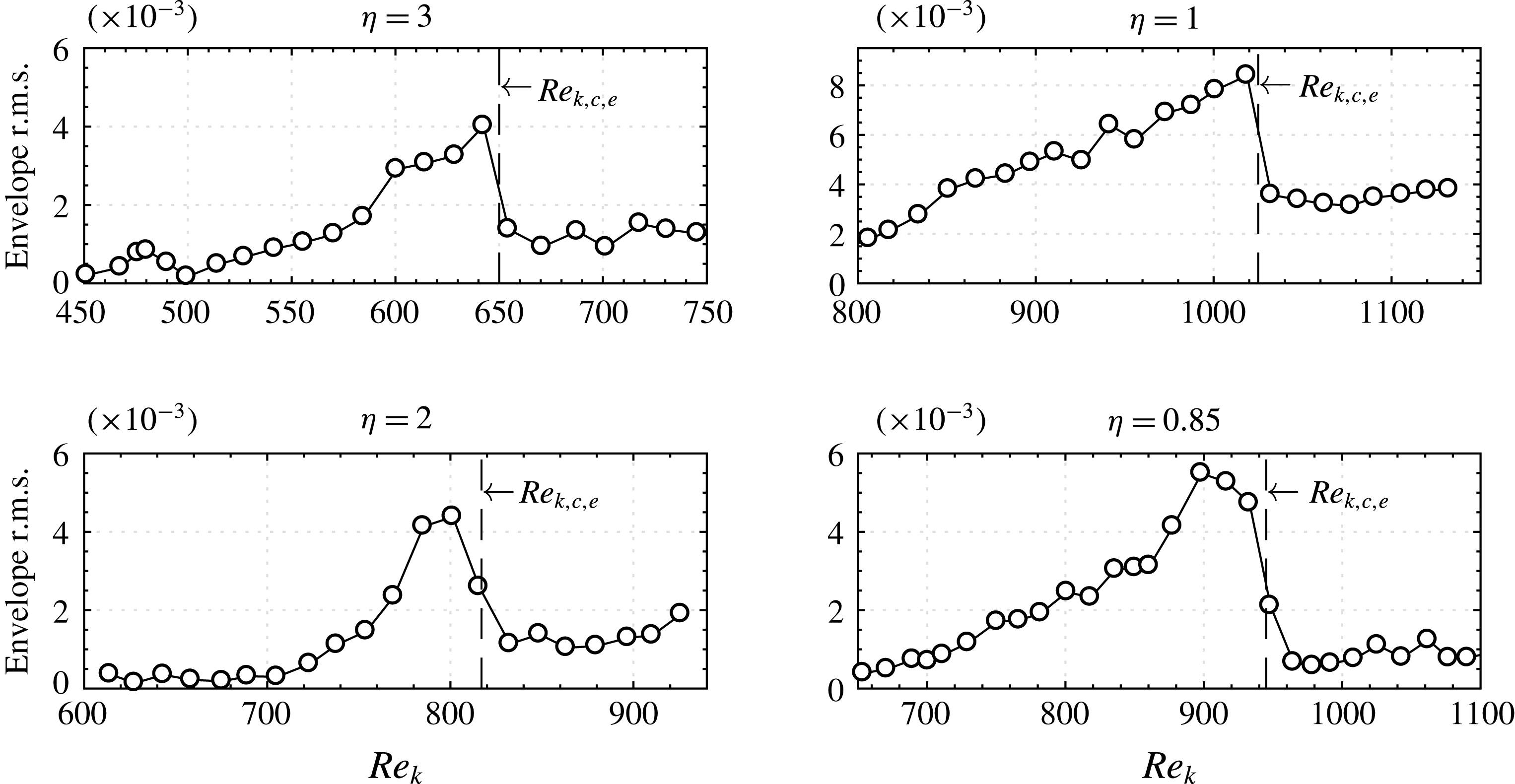
Envelope fluctuation r.m.s. for different aspect ratios.

This procedure has been applied to time traces close to the roughness (
 $x=4$
–7, depending on the aspect ratio) at increasing Reynolds numbers. Results are presented in figure 9, where the envelope r.m.s. is plotted as a function of
 $Re_{k}$
for different aspect ratios. In all cases, the envelope r.m.s. rises initially with increasing
 $Re_{k}$
and then suddenly drops. As already explained, this steep drop can be explained by a changeover of instability mechanism. Similarly to the intermittency threshold, we define the threshold between convective and global instability in the middle of the envelope r.m.s. drop. The experimental critical Reynolds numbers in the contour plots of figure 7 are determined with this procedure. The uncertainty (one standard deviation) is estimated to be
 $\unicode[STIX]{x1D70E}_{Re_{k}}=\pm 15$
and mainly due to measurement errors of
 $U_{e}$
. Minor sources of error are imprecise temperature detection, which has an impact on the kinematic viscosity, manufacturing tolerances of the roughness or local deviations from the Blasius profile.
We now return to figure 7. To illustrate the changeover between convective and global instability further, the fluctuation r.m.s. of the time traces at certain streamwise stations are shown in figure 7(b,d,f,h). The respective streamwise stations are indicated in figure 7(a,c,e,g) with dashed, dash-dotted and dotted lines. For all aspect ratios, the slope of
 $u^{\prime }/U_{e}$
clearly settles to a more constant level beyond
 $Re_{k,c,e}$
, which is again indicated by a solid line in figure 7(b,d,f,h). It can be seen that
 $Re_{k,c,e}$
separates the plots in figure 7 into two distinct regions which are, following nomenclature from theory, denoted by the subcritical and supercritical regime. Plots similar to figure 7 with skewness, kurtosis and intermittency have also been created (not shown), but the r.m.s. remains the most revealing quantity.
 $Re_{k,c,e}$
is not to be confused with the transition Reynolds number, which was introduced in the previous section. In the subcritical regime, background noises from the facility are amplified around and downstream of the roughness, leading to convective disturbance growth, whereas the disturbances in the supercritical regime grow temporally due to a region of self-sustained oscillations. These findings are strong evidence of a global instability in the supercritical regime, in contrast to convective amplification in the subcritical regime.
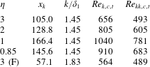
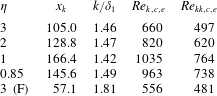
The experimental critical Reynolds numbers obtained through analysis of figures 7 and 9 are compared to the theoretical critical Reynolds numbers in table 2. The case
 $\unicode[STIX]{x1D702}=3$
(F) is from Puckert & Rist (Reference Puckert and Rist2018) and is added for completeness. In all cases, the deviation between experimental and theoretical critical Reynolds number is surprisingly small, particularly when considering all possible errors in the experiment and possible influences of the domain size in the numerical computation. This successful comparison is very strong evidence of a global instability mechanism as predicted theoretically. The experimental detection method with envelopes is fairly simple but powerful to confirm a possible changeover from convective to global instability. Transition detection algorithms as in § 4 or Fransson et al. (Reference Fransson, Brandt, Talamelli and Cossu2005) do not reveal this type of changeover.
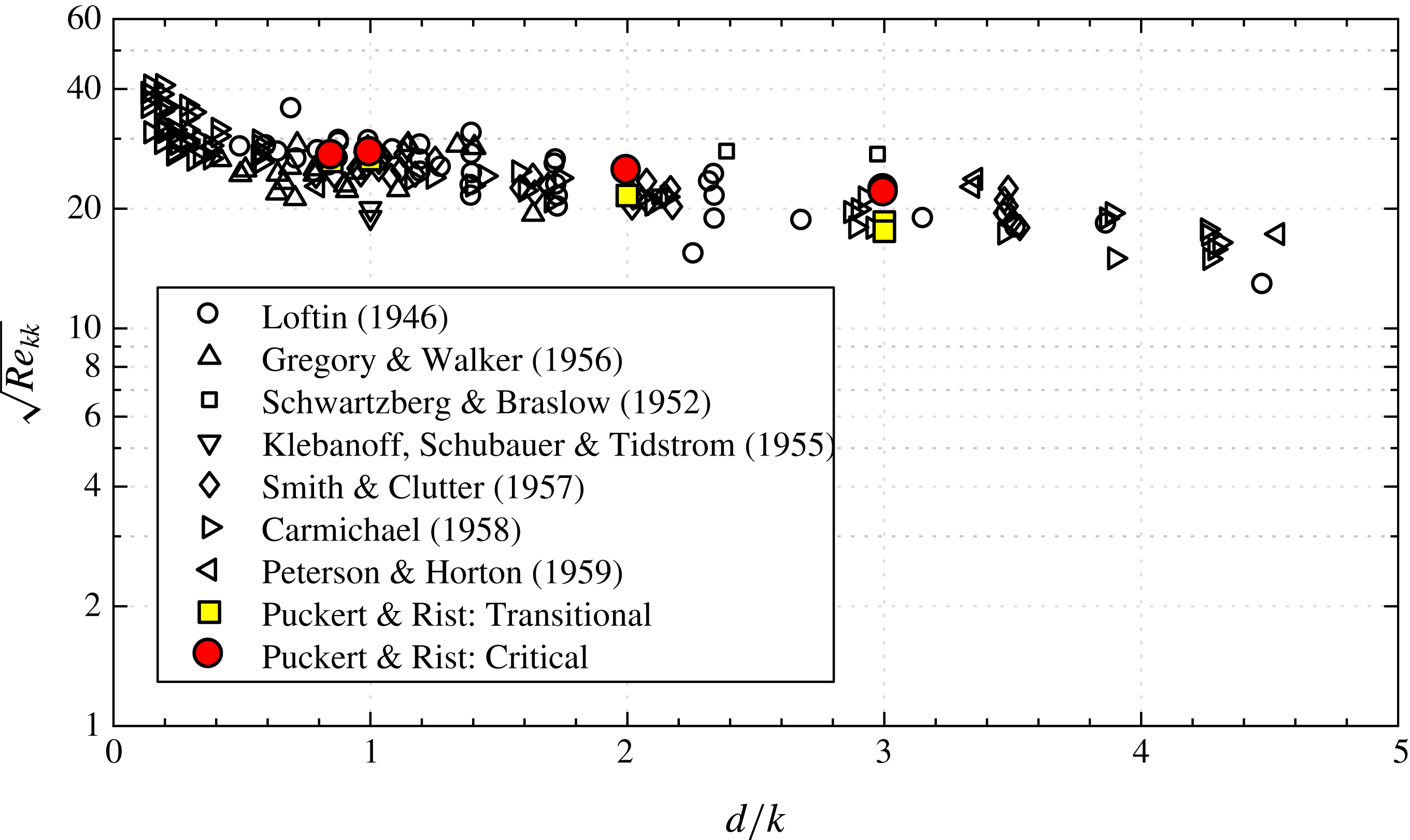
In order to relate the present results to other existing data in the literature, the transition diagram of von Doenhoff & Braslow (Reference von Doenhoff and Braslow1961) has been reproduced in figure 10. The data in this diagram originate from various experimental investigations with different kinds of shapes, isolated elements and arrays of roughness elements from different facilities using different methods. This explains the huge spread of the data but has not reduced the diagram’s popularity in many engineering and scientific applications. Regarding our results, both critical and transition roughness Reynolds numbers from our experiments fit well into this diagram and confirm that our results are in quantitative agreement with the previous literature. The critical Reynolds number is typically higher than the transition Reynolds number and can possibly provide an upper limit when transition occurs at the latest.
Reproduction of the transition diagram by von Doenhoff & Braslow (Reference von Doenhoff and Braslow1961) with critical and transition roughness Reynolds numbers of the present study.

6 Instability mechanism
It has been found that globally unstable oscillations can ignite at the theoretically predicted Reynolds numbers. On the other hand, transition may occur earlier in an experiment before global instability sets in. To understand these two mechanisms, it is helpful to perceive the roughness as an amplifier in the subcritical regime and wavemaker in the supercritical regime. This section will clarify (i) if a linear relation exists between disturbance input and output in the subcritical regime and (ii) if self-sustained modes can cause transition in the supercritical regime. The roughness in the following study has been set up according to the Fransson et al. (Reference Fransson, Brandt, Talamelli and Cossu2005) experiment with
 $\unicode[STIX]{x1D702}=3$
and
 $x_{k}=57.1$
.
6.1 Amplifier
A low subcritical Reynolds number of
 $Re_{k}=430$
was chosen in this experiment to reduce the influence of uncontrolled background noise. The horizontal vibrating wire has been installed at
 $(x,y)=(-7,0.9)$
upstream of the roughness element to introduce controlled disturbances with a forcing frequency of
 $\unicode[STIX]{x1D714}=0.73$
(2 Hz), close to the expected frequency of the stable global mode
 $\unicode[STIX]{x1D714}_{t}=0.8$
at
 $Re_{k}=550$
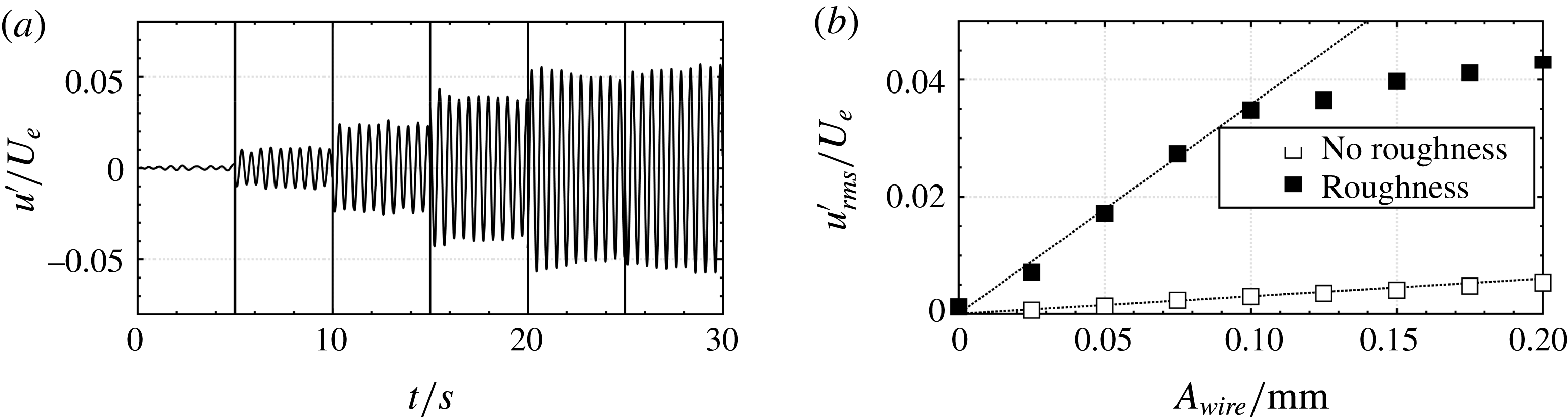
: see Loiseau et al. (Reference Loiseau, Cherubini, Robinet and Leriche2014). This frequency is damped in an undisturbed Blasius boundary layer, but convective amplification may happen in the presence of roughness. Fine mechanical adjustment of the forcing generator’s eccentric wheels has been done to increase the wire oscillation amplitude linearly from 0 to 0.2 mm in steps of 0.025 mm. Figure 11(a) shows 5 s excerpts of the time signals measured at
 $(x,y,z)=(12,1,0)$
for increasing wire oscillation amplitudes. The
 $x$
-position is chosen far enough from the recirculation zone and also far enough from possible transition. From their envelopes it is obvious that the oscillation amplitudes are well controllable by the amplitude of the forcing wire. A more quantitative impression is given in figure 11(b), which shows the fluctuation r.m.s. as a function of wire amplitude for both undisturbed flow and roughness-disturbed flow. In the undisturbed flow, the fluctuation increases linearly with increasing forcing amplitude. This is exactly what is expected from a convective instability that evolves as a wave-like disturbance in the linear regime of the flow:
 $u_{rms}^{\prime }/U_{e}\sim A_{wire}$
where the control parameter is the wire oscillation amplitude
 $A_{wire}$
. The same is true for the roughness-disturbed flow, but linear dependency is only valid up to
 ${\sim}3.5\,\%$
of
 $U_{e}$
. A flow is typically considered linear up to
 $1\,\%$
fluctuation amplitude. However, in practical applications the nonlinear terms can often be neglected even for higher fluctuation amplitudes. The linear relation between forcing amplitude and response amplitude proves that the roughness acts as an amplifier of convective disturbances in the subcritical regime and it can be assumed that the amplification rate is a function of Reynolds number, which has been fixed in this experiment. Here, the controlled disturbances have been amplified by a factor of approximately 12 by the roughness. When the oscillating wire amplitude is further increased and the disturbance amplitude grows beyond
 $3.5\,\%$
of
 $U_{e}$
, nonlinear saturation sets in and the disturbance amplitude increases similarly to a square-root function. Depending on the stability of the downstream boundary layer, this disturbance may develop into turbulence. Variations of frequency lead to similar observations but with different amplification factors.
Forced roughness for
 $(\unicode[STIX]{x1D702},Re_{k})=(3,430)$
with horizontal wire amplitude
 $A_{wire}$
being the control parameter. (a) Time signals with increasing
 $A_{wire}$
every 5 s, (b) r.m.s. of streamwise fluctuation velocities.

6.2 Wavemaker
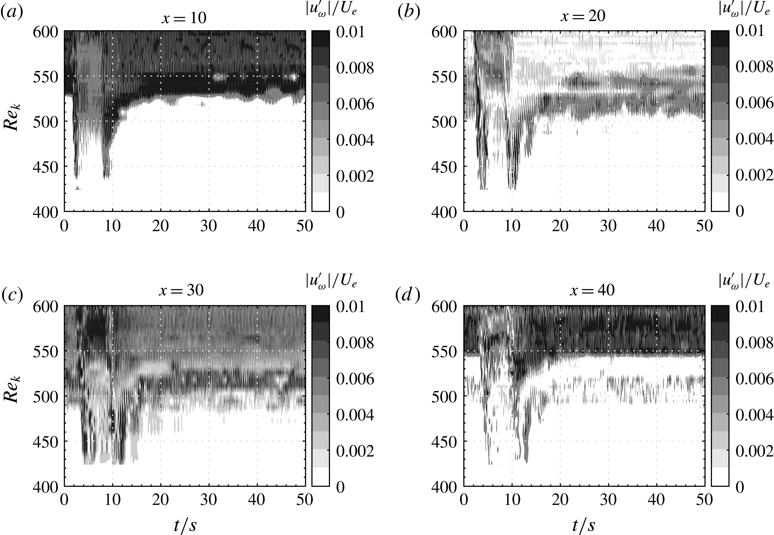
At higher Reynolds numbers, the flow dynamics may change from amplifier to wavemaker due to an unstable self-sustained global mode. If the global instability is purely hydrodynamic without a far-field feedback loop, it necessarily requires a region of local absolute instability within the WKBJ (Wentzel–Kramers–Brillouin–Jeffreys) approximation as shown by Chomaz et al. (Reference Chomaz, Huerre and Redekopp1991) and Monkewitz et al. (Reference Monkewitz, Huerre and Chomaz1993) for general conditions. The region of local absolute instability nurtures a globally unstable mode by shedding upstream and downstream travelling waves, in contrast to local convective instabilities which shed only downstream travelling waves. The temporal evolution of disturbances is investigated here by introducing a wavepacket to the same geometric set-up as previously, but this time the vibrating wire is activated only for the first 6 s and remains off for the remaining 44 s at each measurement point. The probe has been placed at
 $(y,z)=(1,0)$
and four different streamwise stations at
 $x=10$
, 20, 30, 40. The time signals have been recorded five times and ensemble-averaged to reduce random influences. The excitation frequency has been chosen constant at 3 Hz, which is still close to the most receptive frequency expected in the vicinity of the critical Reynolds number, as in the previous section. The higher frequency is due to the higher Reynolds numbers in this experiment. Repeating the acquisition of ensemble-averaged time signals for different Reynolds numbers gives the contour plots of figure 12, where greyscale shows the normalized disturbance magnitudes of ensemble-averaged time signals at different Reynolds numbers. Disturbances in figure 12(a) have peak magnitudes at approximately
 $t=2$
s and 8 s due to transient effects when the wire is switched on and off. The time difference from
 $t=0$
s to 2 s is the time required by the wavepacket to travel from its source to the probe location for the case
 $x=10$
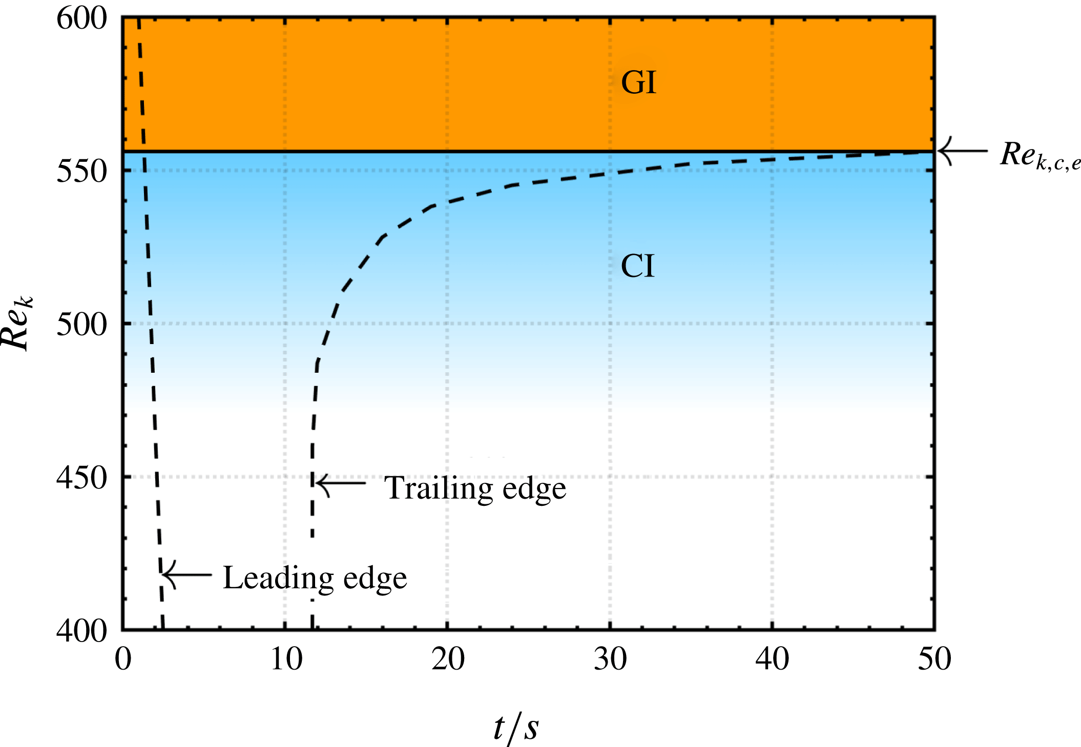
in figure 12(a). At more downstream probe stations, the front and trailing edges of the wavepackets appear at later times, as can be seen in figure 12(a–d), because the wavepackets need to travel over longer distances from their source to the probe. In contrast, the wavepacket front and trailing edges appear earlier when increasing the Reynolds number due to higher convection velocities. Remarkably, the wavepacket trailing edge becomes slower in all plots when the Reynolds number is increased. A similar phenomenon is reported in experiments on rotating disc flows by Lingwood (Reference Lingwood1996) and has been explained by the rise of an absolute instability. The hydrodynamic feedback of upstream and downstream travelling waves is similar here and can be explained by a global instability which is most likely based on a sufficiently large region of absolute instability. The threshold at which this happens has already been detected and the graphs of figure 12 show interesting features at the experimental critical Reynolds number
 $Re_{k,c,e}=556$
. In figure 12(b) the light grey disturbance magnitudes approach this value asymptotically, in (c) there is even a strip of low disturbance magnitude below
 $Re_{k,c,e}=556$
and in (d) this strip becomes thicker, separating the sub- from the supercritical regime most obviously. A precise detection of a threshold is difficult with figure 12, because convective instabilities partially overshadow the changeover to global instability. With this experiment, however, it is shown that the wavepacket trailing edge velocity becomes slower with increasing Reynolds number and is eventually zero or negative. This confirms the existence of a global instability in the dark regions at high Reynolds numbers and convective instability at low Reynolds numbers.
Ensemble-averaged disturbance evolution versus
 $Re_{k}$
at (a)
 $x=10$
, (b)
 $x=20$
, (c)
 $x=30$
and (d)
 $x=40$
.

The coexistence of both convective and global instabilities is schematically drawn in figure 13. In the subcritical regime, convective instabilities (CI) prevail and background noise can be amplified to large amplitudes due to the influence of the roughness. The supercritical regime begins at
 $Re_{k,c,e}$
with a region of global instability (GI). The dashed line symbolizes the evolution of wavepacket leading and trailing edges.
Schematic of instability regions derived from figure 12.

6.3 Varicose versus sinuous mode
It is known from both early and more recent experimental literature that hairpin vortex shedding begins when the Reynolds number is high enough. Hairpin vortices are in general symmetric (varicose) with respect to the streamwise centreline whereas other famous examples of vortex shedding such as the von Kármán street behind 2-D cylinders are antisymmetric (sinuous). In the work of Loiseau et al. (Reference Loiseau, Cherubini, Robinet and Leriche2014), the first unstable global mode is of varicose nature if the roughness aspect ratio is large (
 ${\geqslant}2$
) but sinuous if the aspect ratio is small (1 or below). The agreement for large aspect ratios is good as already shown by Puckert et al. (Reference Puckert, Subasi, Rist and Gunes2015); however, to the authors’ knowledge there is no reported experimental observation of sinuous von Kármán-type vortex shedding behind 3-D roughness elements embedded into a boundary layer. This apparent disagreement with the work of Loiseau et al. (Reference Loiseau, Cherubini, Robinet and Leriche2014) is investigated here by means of PIV.
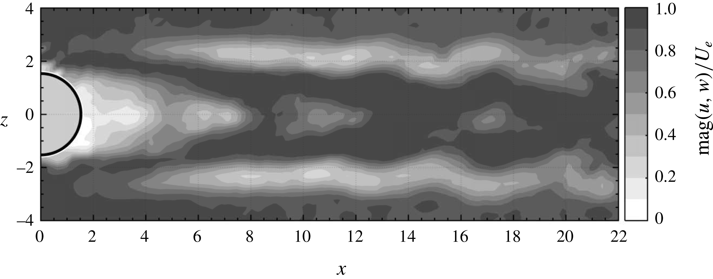
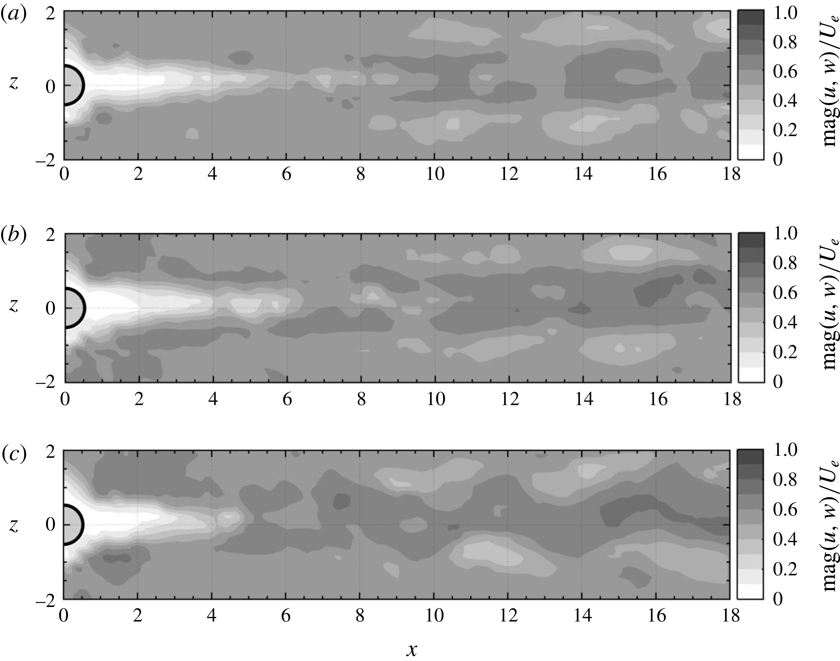
PIV snapshots in the
 $xz$
-plane at the height of the roughness are shown in figures 14 and 15. Greyscale represents the magnitude of the instantaneous in-plane velocity, showing the unsteady streaky wake of the roughness element with the roughness being highlighted light grey for clarity. In the case of a large aspect ratio
 $\unicode[STIX]{x1D702}=3$
(F) (see figure 14), the disturbance symmetry is clearly symmetric with respect to the spanwise centreline. Here, the Reynolds number
 $Re_{k}=700$
is supercritical and thus supports the observation of a leading unstable varicose mode from global LST. However, the symmetric unsteadiness can also be seen for lower Reynolds numbers in the subcritical regime due to amplification of background noise (Puckert & Rist Reference Puckert, Rist, Dillmann, Heller, Krämer, Radespiel and Wagner2016; Bucci et al.
Reference Bucci, Puckert, Andriano, Loiseau, Cherubini, Robinet and Rist2018). Therefore, global and convective instability cannot be clearly distinguished based on mode symmetry for this kind of configuration.
PIV snapshot of the
 $xz$
-plane with
 $\unicode[STIX]{x1D702}=3$
,
 $x_{k}=57.1$
and
 $Re_{k}=700$
.

PIV snapshots of the
 $xz$
-plane with
 $\unicode[STIX]{x1D702}=1$
,
 $x_{k}=166.4$
for (a)
 $Re_{k}=990$
, (b)
 $Re_{k}=1130$
and (c)
 $Re_{k}=1230$
.

Interestingly, this is different for small aspect ratios. Figure 15 shows three snapshots for
 $\unicode[STIX]{x1D702}=1$
at increasing Reynolds numbers. On the one hand, the leading disturbance in figure 15 is clearly symmetric for
 $Re_{k}=990$
(figure 15
a), but on the other hand it becomes antisymmetric for
 $Re_{k}=1230$
(figure 15
c). At an intermediate Reynolds number
 $Re_{k}=1140$
(figure 15
b) the unsteadiness can be understood as a mixture between symmetric and weakly antisymmetric disturbances. Supplementary movie 1, available at https://doi.org/10.1017/jfm.2018.211, demonstrates this changeover even more descriptively. In this experiment, the water channel velocity has been continuously increased to increase the Reynolds number. The free-stream velocity has been measured simultaneously to the PIV measurements with a hot-film probe and with this information, the instantaneous Reynolds number can be provided. The movie shows clearly how the patches of velocity excess and deficit alternate symmetrically in the subcritical regime and antisymmetrically in the supercritical regime. Obviously there must be a changeover in the competition between varicose and sinuous modes when the Reynolds number is increased. Moreover, this changeover occurs close to the theoretical critical Reynolds number
 $Re_{k,c,e}=1040$
and it can be deduced that this observation is due to the unstable global sinuous mode found by Loiseau et al. (Reference Loiseau, Cherubini, Robinet and Leriche2014) for thin aspect ratios. To our knowledge, there has not been any experimental observation of a sinuous disturbance behind isolated roughness elements before, probably due to the strong influence of convective hairpin shedding. At subcritical Reynolds numbers the varicose disturbance dominates because the sinuous global mode is stable. Note that in a physical flow, the two modes coexist and interact nonlinearly with each other. As a result, the sinuous mode can remain hidden in visual observations.
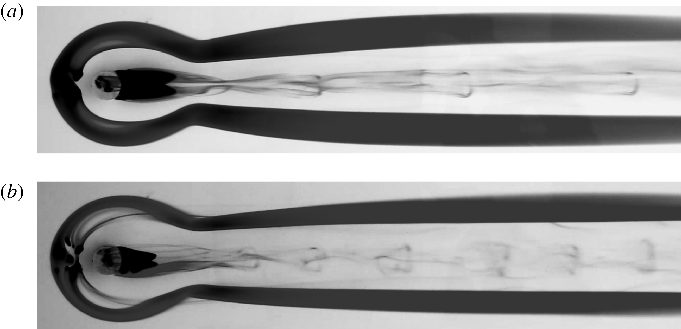
This is demonstrated in figure 16. The pictures show dye streakline visualizations with potassium permanganate around and on top of the roughness with
 $\unicode[STIX]{x1D702}=1$
for two different Reynolds numbers. Hairpin vortices can be seen downstream of the roughness in both the subcritical (figure 16
a) and supercritical regimes (figure 16
b) . Apparently, the varicose hairpin shedding is still active in the supercritical regime despite the globally unstable sinuous mode. Although the basic mechanism of the convective varicose disturbance is different from the global sinuous mode, both disturbances grow to nonlinear saturation at high Reynolds numbers. When the critical Reynolds number is exceeded, the roughness is both amplifier and wavemaker. As a result, there is competition between globally unstable modes from the intrinsic system dynamics and highly amplified external noise. Strong convective growth can outweigh the temporal growth of global modes, and the sinuous oscillation predicted by Loiseau et al. (Reference Loiseau, Cherubini, Robinet and Leriche2014) may thus only dominate in extremely low turbulence environments. When looking closely at the legs of the hairpin vortices in figure 16(b), one can see antisymmetric wiggling submerged in the overall varicose shedding. Similar visualizations have been done for many different roughness elements of various shapes, some of them available in Puckert et al. (Reference Puckert, Subasi, Rist and Gunes2015), and in none of these cases could a clear von Kármán-type vortex shedding be observed. Instead, the shedding seems rather influenced by different modes.
Potassium permanganate visualization of
 $\unicode[STIX]{x1D702}=1$
with (a)
 $Re_{k}=820$
and (b)
 $Re_{k}=1080$
.

The remaining question is whether the stable sinuous mode in the subcritical regime can also be forced similarly to the varicose mode. This is demonstrated in an experiment with symmetric and antisymmetric disturbance sources to force both varicose and sinuous modes. The Reynolds numbers for this experiment are in the subcritical regime and forcing frequencies were chosen according to expected maximum amplification in theory. Either the horizontal or vertical disturbance generator is installed at a time and the goal of this experiment is to demonstrate the sensitivity of the subcritical flow to both varicose and sinuous modes. The roughness with
 $\unicode[STIX]{x1D702}=1$
is again placed at
 $x_{k}=57.1$
and both Reynolds numbers and forcing amplitudes are carefully adjusted to obtain detectable disturbances. The signal-to-noise ratio needs to be as high as possible, but too large Reynolds numbers or forcing amplitudes can lead to uncontrolled vortex shedding which can disturb phase-locked hot-film measurements. It turned out that antisymmetric forcing needs to be much stronger than symmetric forcing due to shear sheltering at the edge of the boundary layer (Hernon, Walsh & McEligot Reference Hernon, Walsh and McEligot2007). Higher excitation amplitudes are thus required.
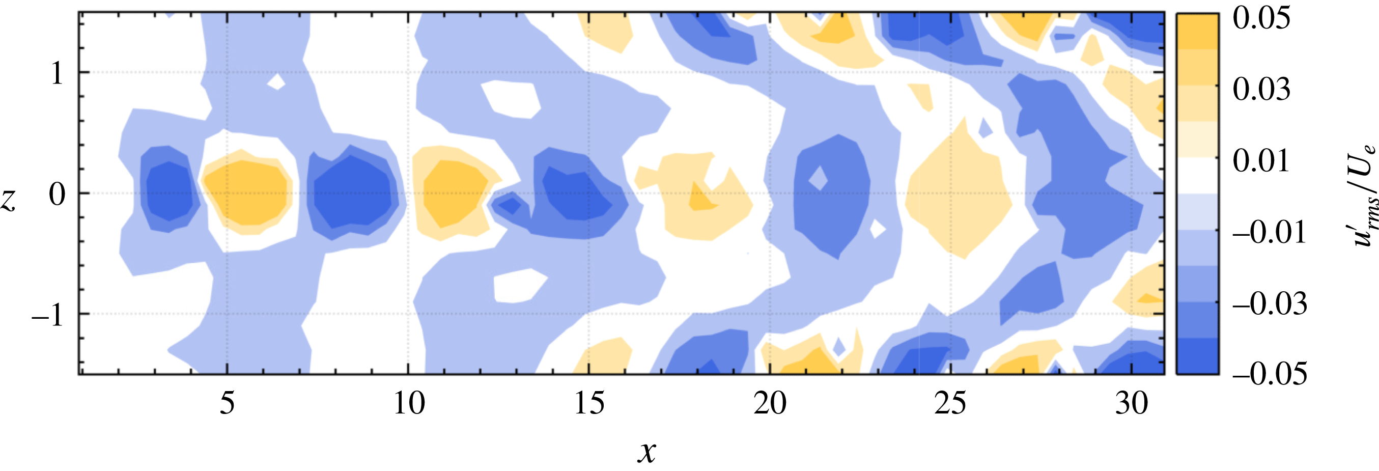
Varicose forcing with
 $f_{f}=0.7~\text{Hz}$
(
 $\unicode[STIX]{x1D714}=0.68$
) at
 $Re_{k}=620$
,
 $\unicode[STIX]{x1D702}=1$
.

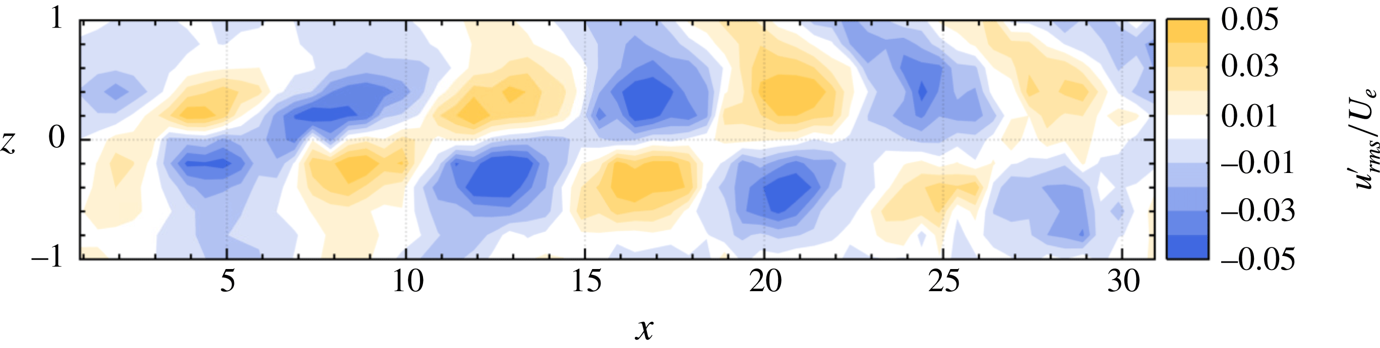
Sinuous forcing with
 $f_{f}=0.65~\text{Hz}$
(
 $\unicode[STIX]{x1D714}=0.56$
) at
 $Re_{k}=694$
,
 $\unicode[STIX]{x1D702}=1$
.

Figures 17 and 18 show the phase-locked measurements in
 $xz$
-slices for the symmetric and antisymmetric forcing, respectively. The spatial resolutions in the
 $x$
and
 $z$
directions are
 $0.5$
and
 $0.25$
, respectively, and the measurement time was 30 s at each position, adding up to a total measurement time of 14 h. Figures 17 and 18 show remarkably well that both sinuous and varicose modes can be forced if parameters are chosen correctly. For the varicose mode this was expected; however, forcing of the sinuous mode is a relatively new technique (see Shin et al.
Reference Shin, Rist and Krämer2015). With this method it could be demonstrated that von Kármán-type instabilities grow when the respective forcing is strong enough. Sinuous modes can thus also develop convectively, similarly to the varicose disturbances which account for hairpin vortex shedding. Although theoretical data of these cases are not at hand, there is qualitative agreement with global mode shapes in Loiseau et al. (Reference Loiseau, Cherubini, Robinet and Leriche2014). Both forced convective instabilities can (quasi-)resonate (Bucci et al.
Reference Bucci, Puckert, Andriano, Loiseau, Cherubini, Robinet and Rist2018) in the roughness wake. The reason for the hairpin vortex shedding in most experimental facilities is therefore due to (i) rather varicose background noise and (ii) higher growth rates of the varicose mode behind the roughness. Nevertheless, the predicted sinuous mode can also be found experimentally with the right environmental conditions.
7 Conclusions
The effects of 3-D cylindrical roughness elements embedded into a laminar boundary layer have been investigated experimentally with particular focus on 3-D global instability. Hot-film measurements revealed that the critical Reynolds number from 3-D global stability theory can also be found experimentally. However, transition does not occur at this critical Reynolds number. Instead, it already begins at lower Reynolds numbers. This is in contrast to what has been reported by Loiseau et al. (Reference Loiseau, Cherubini, Robinet and Leriche2014). It was shown that transition in the subcritical regime is due to convective instabilities whereas the supercritical regime, i.e. beyond the critical Reynolds number, is due to global instability. Further, it could be shown that both sinuous and varicose disturbance modes exist and occur as predicted by theory. For thick roughness elements, the natural disturbances of the unforced flow are symmetric with respect to the spanwise coordinate for both sub- and supercritical conditions, being in agreement with Loiseau et al. (Reference Loiseau, Cherubini, Robinet and Leriche2014). For thin roughness elements, competition between varicose and sinuous modes was found in the proximity of the critical Reynolds number. In the subcritical regime, the unforced flow is disturbed symmetrically by the roughness whereas both antisymmetric wiggling and symmetric hairpin vortices occur in the supercritical regime. This confirms that the roughness is solely an amplifier in the subcritical regime and both amplifier and wavemaker in the supercritical regime. The results from 3-D global LST could be successfully verified in a physical experiment: the mode symmetry and critical Reynolds numbers show good agreement for all the cases studied in this work. As a drawback, the stability of global modes itself is not sufficient yet to fully predict the flow dynamics in highly convective configurations such as in roughness wakes where transient effects can be significant. The critical Reynolds number from theory can thus be understood as a parameter at which instability occurs at the latest.
Acknowledgements
We thank J.-Ch. Robinet, S. Cherubini, J.-Ch. Loiseau and M. A. Bucci for their fruitful cooperation and the anonymous reviewers for their comments. The financial support of the Deutsche Forschungsgemeinschaft (DFG) under reference number RI 680/32-1 is gratefully acknowledged.
Supplementary movie
A supplementary movie is available at https://doi.org/10.1017/jfm.2018.211.
Appendix A. Parameters
Details of the parameter study in § 4.3 are given in table 3 (adapted from the theoretical investigation of Loiseau et al. (Reference Loiseau, Cherubini, Robinet and Leriche2014)). Table 4 provides the corresponding experimental parameters.
Parameters at the critical state in theory (Loiseau et al. Reference Loiseau, Cherubini, Robinet and Leriche2014).

Parameters at the critical state in the experiment.