1 Introduction
Penetrative convection refers to the phenomena that occur whenever convection in a thermally unstable fluid layer penetrates into adjacent stable layers. The unstable fluid layers are often bounded by rigid boundaries in most laboratory experiments on convection. However, stellar convection zones are bounded by stably stratified regions and the understanding of penetration of convection across the interface between stable and unstable layers is of astrophysical importance. For instance, cold plumes from the outer convective zone of the sun penetrate into the upper layers of the tachocline and generate internal gravity waves, this process is thought to play an important role in the turbulent transport of momentum in the tachocline (Dintrans et al. Reference Dintrans, Brandenburg, Nordlund and Stein2005). The observable motions in the outer stable regions of the sun presumably arise from the solar convective zone which is just below them (Leighton Reference Leighton1963). The origin of Jupiter’s zonal winds remains a puzzle and there are two different views: the shallow convection model and the deep convection model (Kong et al. Reference Kong, Zhang, Schubert and Anderson2018). The deep convection model thinks that the zonal flow originates from the penetrative convection that takes place in the deep hydrogen–helium interior (Zhang & Schubert Reference Zhang and Schubert1996, Reference Zhang and Schubert2000). Although Earth’s liquid core is convectively unstable to convection, some studies show that the outermost part of the Earth’s core may be stably stratified (Buffett Reference Buffett2014). The extent of the penetration of convection into the stable layers is important since anomalous depletion of lithium in late stars might be explained if convection penetrates deep enough for the Li–He reaction to occur (Antar Reference Antar1987).
Penetrative convection is usually studied in simplified model problems. Goluskin & van der Poel (Reference Goluskin and van der Poel2016) considered an internally heated fluid layer which is confined between top and bottom plates of equal temperatures. The unstably stratified upper region drives convection that penetrates into the stably stratified lower region. Another commonly used model to study penetrative convection is convection of water near
 $4\,^{\circ }\text{C}$
. Consider a Rayleigh–Bénard convection (RBC) (Ahlers, Grossmann & Lohse Reference Ahlers, Grossmann and Lohse2009; Lohse & Xia Reference Lohse and Xia2010; Chillà & Schumacher Reference Chillà and Schumacher2012) system using water as the working fluid, the temperature of the bottom plate is higher than
 $4\,^{\circ }\text{C}$
while the temperature of the top plate is lower than
 $4\,^{\circ }\text{C}$
. The fluid in the lower layer above the
 $4\,^{\circ }\text{C}$
level is convectively unstable while the upper layer below the
 $4\,^{\circ }\text{C}$
level is gravitationally stable, any convection in the lower, unstable region will penetrate into the stable layer above, and this will lead to the so-called penetrative convection. Convection of water near
 $4\,^{\circ }\text{C}$
was often used as a model problem to study penetrative convection in the past.
The first theoretical work on the subject of penetrative convection considered a layer of water in which the bottom boundary is maintained at
 $0\,^{\circ }\text{C}$
and the top boundary is kept at a temperature larger than
 $4\,^{\circ }\text{C}$
(Veronis Reference Veronis1963). A criterion is built for the onset of instability, and it is demonstrated that the system can become unstable to a finite-amplitude disturbance at values of the Rayleigh number
 $Ra$
less than the critical value of the infinitesimal stability theory. This nonlinear behaviour was later studied by Musman (Reference Musman1968). Moore & Weiss (Reference Moore and Weiss1973) used numerical simulations to extend the small-amplitude solution of penetrative convection to higher
 $Ra$
. Large & Andereck (Reference Large and Andereck2014) experimentally investigate penetrative RBC, they found that the conduction–convection transition is hysteretic in nature, and the flow undergoes secondary transitions to either hexagonal cellular or longitudinal roll states at higher
 $Ra$
. Hu, Li & Wu (Reference Hu, Li and Wu2015) investigated RBC of water near
 $4\,^{\circ }\text{C}$
in a cubical cavity with different thermal boundaries on the side walls and found that there are multiple flow pattern coexisting and that the hysteresis phenomenon occurs during the flow pattern transition.
Most of the previous works are conducted at relatively low
 $Ra$
where the flow is laminar. There are less works devoted to turbulent penetrative convection. Lecoanet et al. (Reference Lecoanet, Le Bars, Burns, Vasil, Brown, Quataert and Oishi2015) studied internal gravity wave excitation by convection of water near
 $4\,^{\circ }\text{C}$
at
 $Ra=5.8\times 10^{7}$
using two-dimensional (2-D) simulations. A recent work (Toppaladoddi & Wettlaufer Reference Toppaladoddi and Wettlaufer2018) investigated 2-D penetrative convection at relatively high Rayleigh numbers
 $10^{6}\leqslant Ra\leqslant 10^{8}$
using the lattice Boltzmann method, where the authors adopted periodic conditions in the horizontal direction with Prandtl numbers of 1 and 11.6. More recently, Couston et al. (Reference Couston, Lecoanet, Favier and Le Bars2018) numerically investigated 2-D penetrative convection with horizontal periodic conditions and found that a periodic, oscillating mean flow spontaneously develops from turbulently generated internal waves. The non-Oberbeck–Boussinesq (NOB) nature of water near
 $4\,^{\circ }\text{C}$
will cause a top–down symmetry breaking, leading to a shift of centre temperature
 $\unicode[STIX]{x1D703}_{c}$
, i.e.
 $\unicode[STIX]{x1D703}_{c}$
will deviate from that of the Oberbeck–Boussinesq (OB) case. This deviation has been investigated in RBC with NOB effects caused by large temperature differences (Zhang, Childress & Libchaber Reference Zhang, Childress and Libchaber1997; Ahlers et al.
Reference Ahlers, Brown, Araujo, Funfschilling, Grossmann and Lohse2006, Reference Ahlers, Araujo, Funfschilling, Grossmann and Lohse2007; Sameen, Verzicco & Sreenivasan Reference Sameen, Verzicco and Sreenivasan2008, Reference Sameen, Verzicco and Sreenivasan2009; Sugiyama et al.
Reference Sugiyama, Calzavarini, Grossmann and Lohse2009; Horn, Shishkina & Wagner Reference Horn, Shishkina and Wagner2013; Horn & Shishkina Reference Horn and Shishkina2014; Weiss et al.
Reference Weiss, He, Ahlers, Bodenschatz and Shishkina2018). However, there is still a lack of systematic studies on the centre temperature
 $\unicode[STIX]{x1D703}_{c}$
in turbulent penetrative RBC of water near
 $4\,^{\circ }\text{C}$
. We try to fill this gap and report a universal relationship of
 $\unicode[STIX]{x1D703}_{c}$
with the density inversion parameter
 $\unicode[STIX]{x1D703}_{m}$
. The ratio of the top and bottom thermal boundary-layer (BL) thicknesses
 $F_{\unicode[STIX]{x1D706}}=\unicode[STIX]{x1D706}_{t}^{\unicode[STIX]{x1D703}}/\unicode[STIX]{x1D706}_{b}^{\unicode[STIX]{x1D703}}$
, the normalized Nusselt number
 $Nu(\unicode[STIX]{x1D703}_{m})/Nu(0)$
and Reynolds number
 $Re(\unicode[STIX]{x1D703}_{m})/Re(0)$
are also found to have universal relationships with
 $\unicode[STIX]{x1D703}_{m}$
which seem to be independent of
 $Ra$
.
The rest of the paper is organized as follows. We first briefly describe the governing equations and numerical methods in § 2. Section 3 presents and discusses the universal relationships of
 $F_{\unicode[STIX]{x1D706}}$
,
 $\unicode[STIX]{x1D703}_{c}$
, normalized Nusselt number
 $Nu(\unicode[STIX]{x1D703}_{m})/Nu(0)$
and normalized Reynolds number
 $Re(\unicode[STIX]{x1D703}_{m})/Re(0)$
with respect to
 $\unicode[STIX]{x1D703}_{m}$
. Finally, we summarize our findings in § 4, and the simulation details are tabulated in the Appendix.
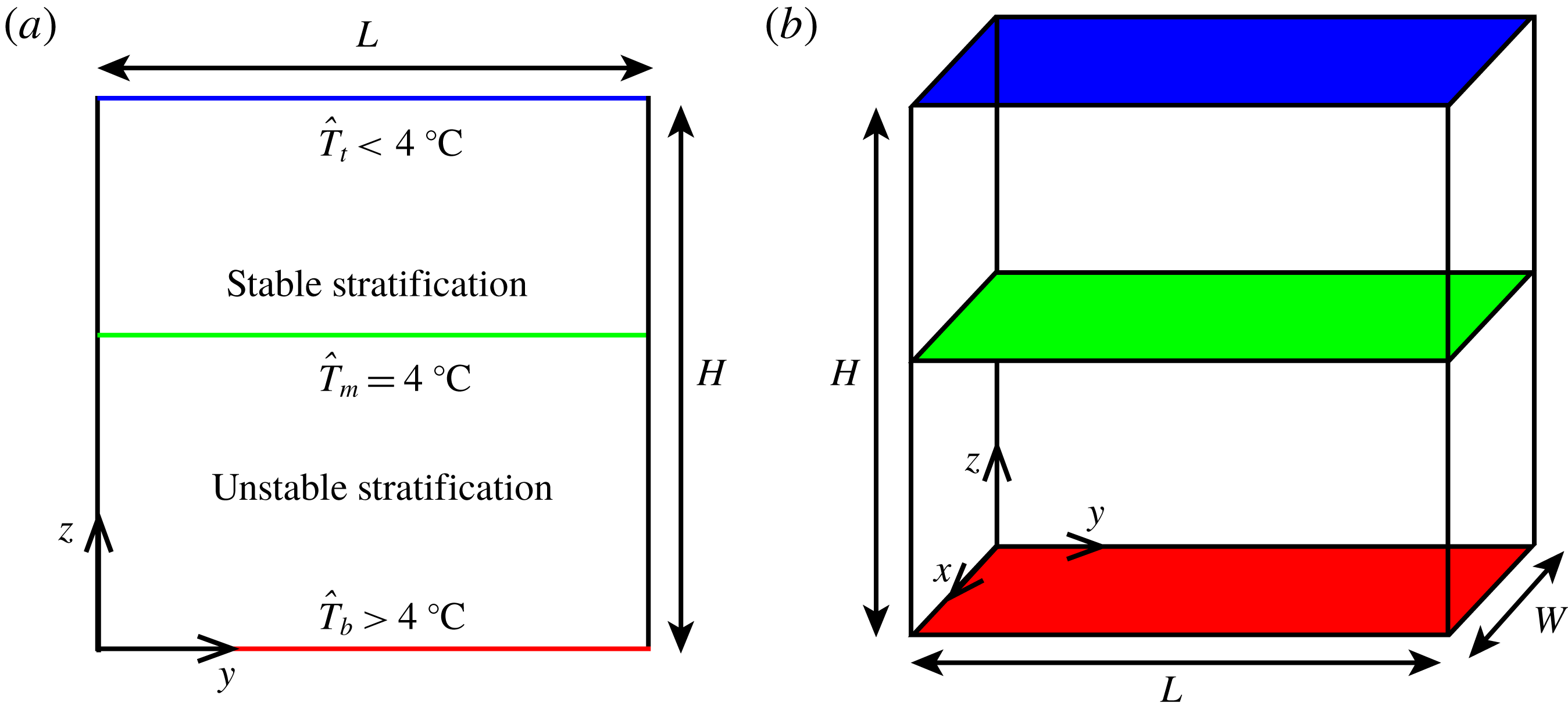
Sketch of (a) 2-D and (b) three-dimensional (3-D) configurations for penetrative Rayleigh–Bénard convection.

2 Numerical procedures
The problem is sketched in figure 1, the temperature of the bottom plate
 $\hat{T}_{b}$
(quantities marked with a circumflex are dimensional) is higher than
 $4\,^{\circ }\text{C}$
while the temperature of the top plate is lower than
 $4\,^{\circ }\text{C}$
. The side walls are insulated. We assume thermophysical properties to be constant except the density in the buoyancy term. The nonlinear relationship of density with temperature for cold water near
 $4^{\circ }$
is described as
 $\hat{\unicode[STIX]{x1D70C}}=\hat{\unicode[STIX]{x1D70C}}_{m}(1-\hat{\unicode[STIX]{x1D6FC}}|\hat{T}-\hat{T}_{m}|^{q})$
(Gebhart & Mollendorf Reference Gebhart and Mollendorf1977), where
 $\hat{\unicode[STIX]{x1D70C}}_{m}\approx 1000~\text{kg}~\text{m}^{-3}$
is the maximum density at the temperature
 $\hat{T}_{m}=4\,^{\circ }\text{C}$
, the isobaric thermal expansion coefficient
 $\hat{\unicode[STIX]{x1D6FC}}=9.30\times 10^{-6}~(\text{}^{\circ }\text{C})^{-q}$
, where
 $q=1.895$
. The dimensionless governing equations of this problem read
 $$\begin{eqnarray}\displaystyle & \displaystyle \unicode[STIX]{x1D735}\boldsymbol{\cdot }\boldsymbol{u}=0 & \displaystyle\end{eqnarray}$$
 $$\begin{eqnarray}\displaystyle & \displaystyle \frac{\unicode[STIX]{x2202}\boldsymbol{u}}{\unicode[STIX]{x2202}t}+\boldsymbol{u}\boldsymbol{\cdot }\unicode[STIX]{x1D735}\boldsymbol{u}=-\unicode[STIX]{x1D735}p+\sqrt{\frac{Pr}{Ra}}\unicode[STIX]{x1D6FB}^{2}\boldsymbol{u}+|\unicode[STIX]{x1D703}-\unicode[STIX]{x1D703}_{m}|^{q}\boldsymbol{e}_{z} & \displaystyle\end{eqnarray}$$
 $$\begin{eqnarray}\displaystyle & \displaystyle \frac{\unicode[STIX]{x2202}\unicode[STIX]{x1D703}}{\unicode[STIX]{x2202}t}+\boldsymbol{u}\boldsymbol{\cdot }\unicode[STIX]{x1D735}\unicode[STIX]{x1D703}=\frac{1}{\sqrt{RaPr}}\unicode[STIX]{x1D6FB}^{2}\unicode[STIX]{x1D703}, & \displaystyle\end{eqnarray}$$
where
 $\boldsymbol{u}$
,
 $\unicode[STIX]{x1D703}$
and
 $p$
are the velocity, temperature and pressure, respectively. For non-dimensionalization, we choose
 ${\hat{H}}$
and
 $\hat{U} =({\hat{g}}\hat{\unicode[STIX]{x1D6FC}}\unicode[STIX]{x0394}\hat{T}^{q}{\hat{H}})^{1/2}$
as reference length and velocity, where
 ${\hat{g}}$
is the gravitational acceleration,
 $\unicode[STIX]{x0394}\hat{T}=\hat{T}_{b}-\hat{T}_{t}$
is the temperature difference. The reference time is free-fall time
 $\hat{t}_{f}={\hat{H}}/\hat{U}$
. Temperature is non-dimensionalized as
 $\unicode[STIX]{x1D703}=(\hat{T}-\hat{T}_{t})/(\hat{T}_{b}-\hat{T}_{t})$
. The three main control parameters are the Prandtl number
 $Pr$
, the Rayleigh number
 $Ra$
, the density inversion parameter
 $\unicode[STIX]{x1D703}_{m}$
and they are defined as
 $$\begin{eqnarray}\displaystyle Pr=\frac{\hat{\unicode[STIX]{x1D708}}}{\hat{\unicode[STIX]{x1D705}}},\quad Ra=\frac{{\hat{g}}\hat{\unicode[STIX]{x1D6FC}}(\hat{T}_{b}-\hat{T}_{t})^{q}{\hat{H}}^{3}}{\hat{\unicode[STIX]{x1D708}}\hat{\unicode[STIX]{x1D705}}},\quad \unicode[STIX]{x1D703}_{m}=\frac{\hat{T}_{m}-\hat{T}_{t}}{\hat{T}_{b}-\hat{T}_{t}}, & & \displaystyle\end{eqnarray}$$
where
 $\hat{\unicode[STIX]{x1D705}}$
is the thermal diffusivity, and
 $\hat{\unicode[STIX]{x1D708}}$
the kinematic viscosity;
 $\unicode[STIX]{x1D703}_{m}$
is an important parameter that describes the density maximum effect, quantifying the location of
 $\hat{T}_{m}$
with respect to wall temperatures
 $\hat{T}_{t}$
and
 $\hat{T}_{b}$
. For
 $\unicode[STIX]{x1D703}_{m}=0$
, the top plate is
 $4\,^{\circ }\text{C}$
, and the situation is quite similar to the OB approximation. For
 $\unicode[STIX]{x1D703}_{m}=1$
, the bottom plate is
 $4\,^{\circ }\text{C}$
, and the flow is in the pure conduction state for any
 $Ra$
. Another control parameter is the aspect ratio. For the 2-D configuration, the aspect ratio is defined as
 $\unicode[STIX]{x1D6E4}=\hat{L}/{\hat{H}}$
. For the 3-D configuration, the dimensionless length is fixed to 1 and the aspect ratio is defined as
 $\unicode[STIX]{x1D6E4}_{3}={\hat{W}}/{\hat{H}}$
.
The governing equations are solved numerically by an in-house code lMn2d/3d (Xia et al. Reference Xia, Wan, Liu, Wang and Sun2016). Since our code has been validated and used to study various convection problem before (Wang et al. Reference Wang, Xu, Xia, Wan and Sun2017; Liu et al. Reference Liu, Xia, Yan, Wan and Sun2018; Wang et al. Reference Wang, Wan, Yan and Sun2018a ,Reference Wang, Xia, Wang, Sun, Zhou and Wan b , Reference Wang, Wan, Yan and Sun2019a ,Reference Wang, Xia, Yan, Sun and Wan b ), we only give its main features here. All spatial terms are discretized using a second-order central difference scheme. Non-uniform grids with clustered points near the walls are used. Time integration is accomplished using an Adams–Bashforth scheme for the nonlinear terms and a Crank–Nicolson scheme for the viscous and diffusion terms. Multi-grid strategy is used to solve the pressure Poisson equation.
The
 $Pr$
is fixed to 11.57 corresponding to water at
 $4\,^{\circ }\text{C}$
. We simulate 2-D cases in the range of
 $10^{7}\leqslant Ra\leqslant 10^{10}$
and 3-D cases for
 $Ra=10^{8}$
and
 $10^{9}$
. Grids which satisfy resolution requirement of direct numerical simulations (DNS) (Shishkina et al.
Reference Shishkina, Stevens, Grossmann and Lohse2010) are used. The details of the main simulations are tabulated in the Appendix. For all the simulations, we generally perform at least 1600 free-fall time units. We waited at least 800 free-fall time units before starting to average in order to ensure all transients have been dissipated, and the
 $Nu$
and
 $Re$
are averaged for at least 800 free-fall time units. For large
 $\unicode[STIX]{x1D703}_{m}$
close to 0.9, longer-time simulations are needed to reach statistically steady state (Toppaladoddi & Wettlaufer Reference Toppaladoddi and Wettlaufer2018). For example, for the 2-D case with
 $Ra=5\times 10^{8},\unicode[STIX]{x1D703}_{m}=0.9,\unicode[STIX]{x1D6E4}=1$
, we preformed 30 000 free-fall time units for the flow to become statistically steady, and another 10 000 free-fall time units are simulated for the time average. The results are also compared with OB cases where we set
 $q=1$
and
 $\unicode[STIX]{x1D703}_{m}=0$
. Note that for the penetrative case with
 $\unicode[STIX]{x1D703}_{m}=0$
, the flow is similar to OB cases, but it cannot fully recover to OB case since
 $q=1.895$
, and the top–bottom symmetry is still broken. For the OB case, the initial conditions are conduction states superposed with a small perturbation added to the temperature, while for the penetrative cases, we generally use fully developed flow fields for the OB cases as initial conditions.
3 Results and discussion
3.1 Flow organization and centre temperature
(a–c) Instantaneous temperature fields superimposed with velocity vectors for
 $Ra=10^{9}$
for 2-D cases with
 $\unicode[STIX]{x1D6E4}=1$
. (d–f) Time-averaged kinetic energy
 $1/2(v^{2}+w^{2})$
distribution superimposed with velocity vectors for
 $Ra=10^{9}$
for 2-D cases with
 $\unicode[STIX]{x1D6E4}=1$
. (g–h) Instantaneous temperature fields for
 $Ra=10^{9}$
for 3-D cases with
 $\unicode[STIX]{x1D6E4}_{3}=1/2$
. (a,d,g) OB. (b,e,h)
 $\unicode[STIX]{x1D703}_{m}=0.4$
. (c,f,i)
 $\unicode[STIX]{x1D703}_{m}=0.8$
. The black lines in (b,c) and white lines in (e,f) denote the location where the temperature is
 $4^{\circ }$
.

Figure 2 shows instantaneous temperature (a–c)/time-averaged kinetic energy
 $0.5(v^{2}+w^{2})$
(d–f) fields superimposed with velocity vectors for 2-D cases with
 $Ra=10^{9},\unicode[STIX]{x1D6E4}=1$
, and instantaneous temperature fields for 3-D cases with
 $Ra=10^{9},\unicode[STIX]{x1D6E4}_{3}=1/2$
(g–i). It is seen that a large-scale circulation (LSC) which spans the whole size of the convection cell exists for the OB cases as shown in figure 2(a,d,g). For the penetrative cases, due to the penetration of the lower hotter unstable fluid layer into the upper stably stratified layer, the temperature in the bulk increases compared to that of the OB cases. For relatively small
 $\unicode[STIX]{x1D703}_{m}$
, the fluid in the lower layer can penetrate into the whole part of the upper layer as shown in figure 2(b,e,h). However, for large
 $\unicode[STIX]{x1D703}_{m}$
, vigorous convection cannot happen in the whole cell, and the flow is stably stratified near the top plate as depicted in figure 2(c,f,i). The convection is very weak near the top plate, and heat is transferred mainly by thermal conduction in this region. This stably stratified temperature field is somewhat similar to the stably stratified angular velocity field in counter-rotating Taylor–Couette flow where Rayleigh-stable zones exist near the outer cylinder (Van Gils et al.
Reference Van Gils, Huisman, Bruggert, Sun and Lohse2011; Ostilla-Mónico et al.
Reference Ostilla-Mónico, Stevens, Grossmann, Verzicco and Lohse2013, Reference Ostilla-Mónico, van der Poel, Verzicco, Grossmann and Lohse2014). The black lines in figure 2(b,c) denote the location where the temperature is
 $4\,^{\circ }\text{C}$
. Some fluctuations are observed due to the interaction between lower convection region and upper stably stratified region. The white lines in figure 2(e,f) also depict the location at which the temperature is
 $4\,^{\circ }\text{C}$
, but in time-averaged sense. It is clearly shown that the fluctuations disappear after time averaging. In figure 2(d–f), one can also observe that the velocity magnitude decreases with increasing
 $\unicode[STIX]{x1D703}_{m}$
.
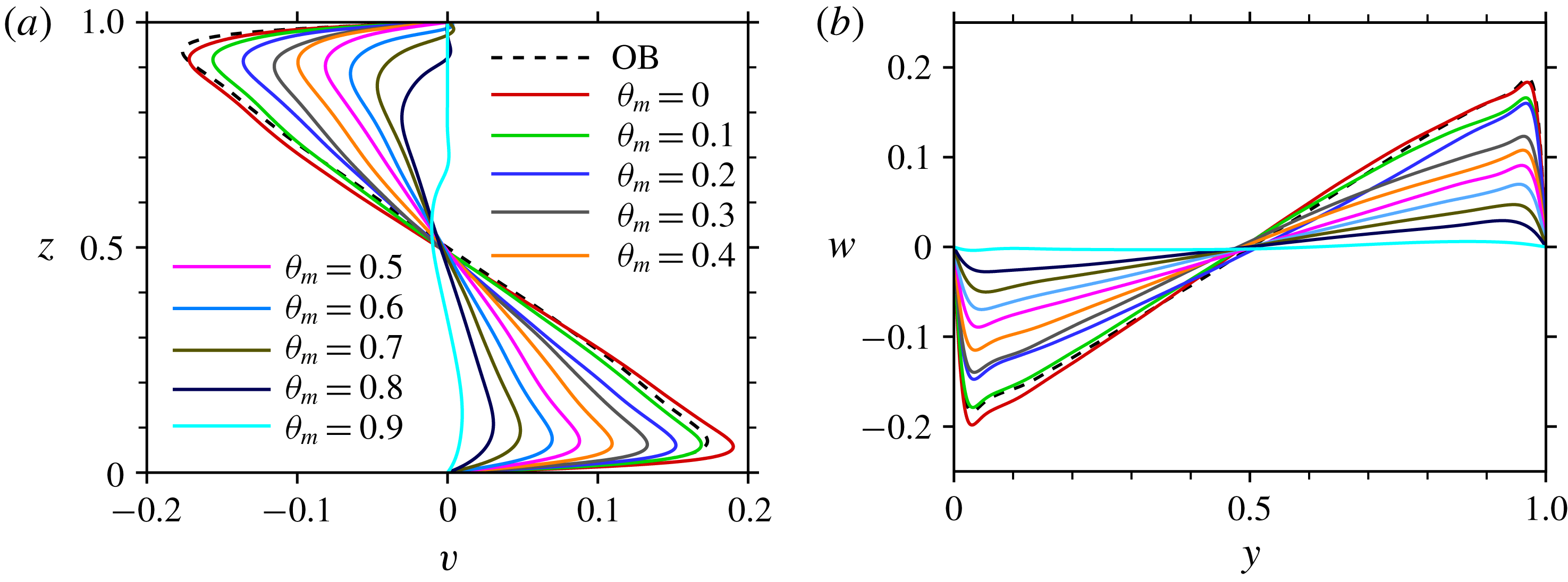
We now quantitatively investigate velocity profiles. Figure 3(a) shows time-averaged horizontal velocity
 $v$
profile at the line
 $y=0.5$
for 2-D cases with
 $Ra=10^{9},\unicode[STIX]{x1D6E4}=1$
. The profile is symmetrical for the OB case. For
 $\unicode[STIX]{x1D703}_{m}=0$
, the profile is very close to the OB case, however, we can see that the peak horizontal velocity near the bottom plate is slightly increased compared to the OB case, while it decreases a little near the top plate. As
 $\unicode[STIX]{x1D703}_{m}$
increases, the fluid motion is obviously weakened, and the horizontal velocity peak decreases monotonically with increasing
 $\unicode[STIX]{x1D703}_{m}$
, the velocity boundary layers that form near the top plate can still be clearly identified for not too large
 $\unicode[STIX]{x1D703}_{m}$
. As
 $\unicode[STIX]{x1D703}_{m}$
increases further to
 $0.7,0.8$
, there is a region where
 $v$
is around 0 near the top plate. This corresponds to the stably stratified flow structure for relative large
 $\unicode[STIX]{x1D703}_{m}$
. For
 $\unicode[STIX]{x1D703}_{m}=0.9$
, there exist flow reversals of the LSC (Sugiyama et al.
Reference Sugiyama, Ni, Stevens, Chan, Zhou, Xi, Sun, Grossmann, Xia and Lohse2010), thus we only average counter-clockwise circulation for this case. It is seen that convection only happens at the lower layer with
 $z$
approximately smaller than 0.7. Figure 3(b) shows the time-averaged vertical velocity
 $w$
profile at the line
 $z=0.5$
. For
 $\unicode[STIX]{x1D703}_{m}=0$
, the profile is also asymmetrical, and the velocity peak is larger than the OB case near the left plate. The vertical velocity peak is also found to decrease with increasing
 $\unicode[STIX]{x1D703}_{m}$
.
Time-averaged velocity profiles for
 $Ra=10^{9}$
for 2-D cases with
 $\unicode[STIX]{x1D6E4}=1$
(a)
 $v$
profile at
 $y=0.5$
for different
 $\unicode[STIX]{x1D703}_{m}$
; (b)
 $w$
profile at
 $z=0.5$
for different
 $\unicode[STIX]{x1D703}_{m}$
.

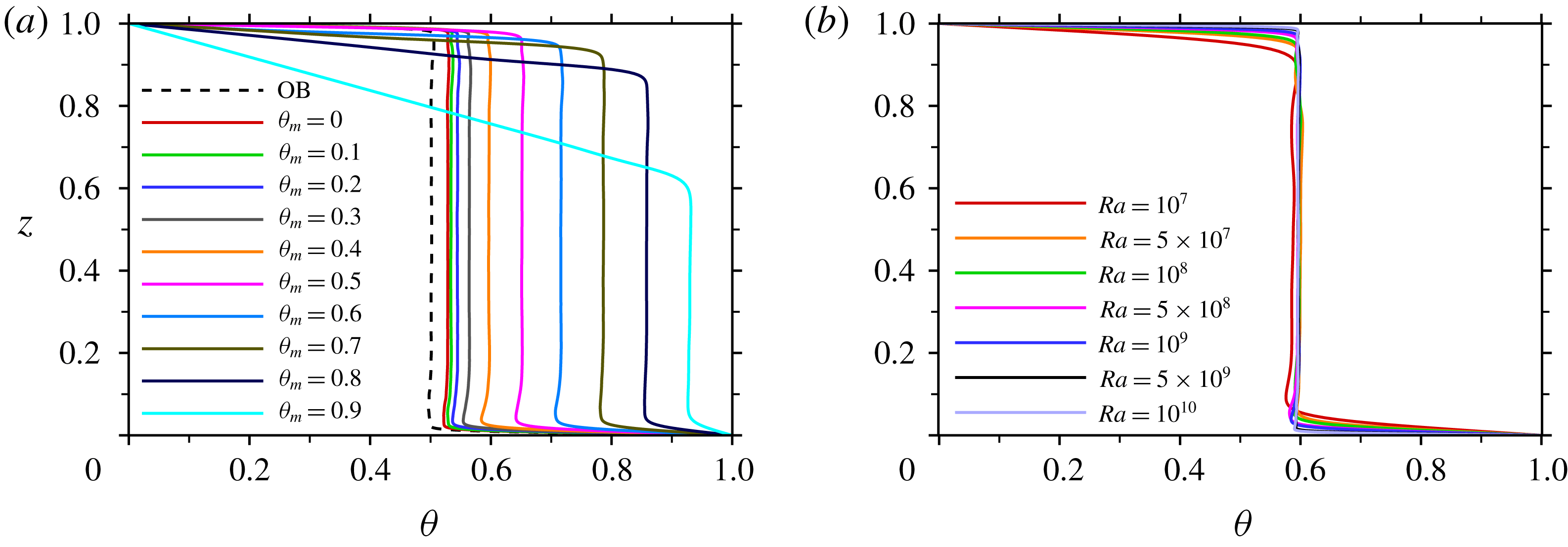
We now investigate thermal boundary layers and centre temperature. In figure 4(a) we show time-averaged temperature profiles at the location of
 $y=0.5$
for the 2-D case with
 $Ra=10^{9},\unicode[STIX]{x1D6E4}=1$
. For the OB case, the temperature at the centre
 $\unicode[STIX]{x1D703}_{c}$
is the arithmetic mean of the top- and bottom-plate temperatures. For
 $\unicode[STIX]{x1D703}_{m}=0$
, it is clearly seen that
 $\unicode[STIX]{x1D703}_{c}$
is enhanced compared to that of the OB case. With increasing
 $\unicode[STIX]{x1D703}_{m}$
, the thermal BLs become thicker and
 $\unicode[STIX]{x1D703}_{c}$
becomes larger. It is also evident that the top BL is thicker than that of the bottom BL. Figure 4(b) shows time-averaged temperature profiles at the location of
 $y=0.5$
for the 2-D cases with
 $\unicode[STIX]{x1D703}_{m}=0.4,\unicode[STIX]{x1D6E4}=1$
. An interesting feature is that, although the thermal BLs become thinner with increasing
 $Ra$
, the bulk temperature is nearly unchanged for all
 $Ra$
.
Time-averaged temperature profiles at
 $y=0.5$
for 2-D cases with
 $\unicode[STIX]{x1D6E4}=1$
for (a)
 $Ra=10^{9}$
with different
 $\unicode[STIX]{x1D703}_{m}$
and (b)
 $\unicode[STIX]{x1D703}_{m}=0.4$
with different
 $Ra$
.

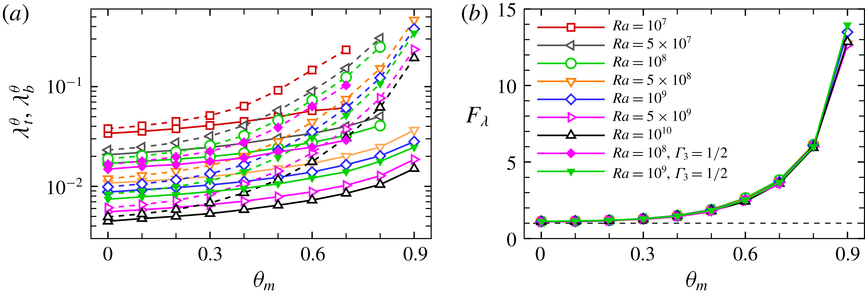
(a) Bottom thermal boundary-layer thickness
 $\unicode[STIX]{x1D706}_{b}^{\unicode[STIX]{x1D703}}$
(solid lines) and top thermal boundary-layer thickness
 $\unicode[STIX]{x1D706}_{t}^{\unicode[STIX]{x1D703}}$
(dashed lines) as a function of
 $\unicode[STIX]{x1D703}_{m}$
for 2-D cases with
 $\unicode[STIX]{x1D6E4}=1$
and 3-D cases with
 $\unicode[STIX]{x1D6E4}_{3}=1/2$
. (b) The ratio of the top and bottom thermal BL thicknesses
 $F_{\unicode[STIX]{x1D706}}=\unicode[STIX]{x1D706}_{t}^{\unicode[STIX]{x1D703}}/\unicode[STIX]{x1D706}_{b}^{\unicode[STIX]{x1D703}}$
as a function of
 $\unicode[STIX]{x1D703}_{m}$
for 2-D cases with
 $\unicode[STIX]{x1D6E4}=1$
and 3-D cases with
 $\unicode[STIX]{x1D6E4}_{3}=1/2$
.

We then quantify the asymmetrical feature of the two thermal BLs. Figure 5(a) illustrates top and bottom thermal BL thicknesses versus
 $\unicode[STIX]{x1D703}_{m}$
for both 2-D cases with
 $\unicode[STIX]{x1D6E4}=1$
and 3-D cases with
 $\unicode[STIX]{x1D6E4}_{3}=1/2$
. The thickness of top thermal BL
 $\unicode[STIX]{x1D706}_{t}^{\unicode[STIX]{x1D703}}$
and bottom thermal BL
 $\unicode[STIX]{x1D706}_{b}^{\unicode[STIX]{x1D703}}$
are defined as (Horn et al.
Reference Horn, Shishkina and Wagner2013)
 $$\begin{eqnarray}\displaystyle \unicode[STIX]{x1D706}_{t}^{\unicode[STIX]{x1D703}}=\frac{\unicode[STIX]{x1D703}_{t}-\unicode[STIX]{x1D703}_{c}}{\unicode[STIX]{x2202}_{z}\langle \unicode[STIX]{x1D703}\rangle _{A,t}|_{z=1}},\quad \unicode[STIX]{x1D706}_{b}^{\unicode[STIX]{x1D703}}=\frac{\unicode[STIX]{x1D703}_{c}-\unicode[STIX]{x1D703}_{b}}{\unicode[STIX]{x2202}_{z}\langle \unicode[STIX]{x1D703}\rangle _{A,t}|_{z=0}}, & & \displaystyle\end{eqnarray}$$
where
 $\unicode[STIX]{x1D703}_{t}=0/\unicode[STIX]{x1D703}_{b}=1$
are the temperatures at the top/bottom plates.
 $\langle \rangle _{A,t}$
denotes average over any horizontal plane (3-D)/line (2-D) and in time. One can clearly see that both the two quantities increase with increasing
 $\unicode[STIX]{x1D703}_{m}$
, and
 $\unicode[STIX]{x1D706}_{t}^{\unicode[STIX]{x1D703}}$
increases more rapidly. Figure 5(b) shows the ratio of the top and bottom thermal BL thicknesses
 $F_{\unicode[STIX]{x1D706}}=\unicode[STIX]{x1D706}_{t}^{\unicode[STIX]{x1D703}}/\unicode[STIX]{x1D706}_{b}^{\unicode[STIX]{x1D703}}$
. It can be seen that
 $F_{\unicode[STIX]{x1D706}}$
is an increasing function of
 $\unicode[STIX]{x1D703}_{m}$
, and it rapidly increases for large
 $\unicode[STIX]{x1D703}_{m}$
near 0.9, due to the fact that the stably stratified flow structures appear for large
 $\unicode[STIX]{x1D703}_{m}$
, as shown in figure 2(c,f), leading to a much thicker thermal BL near the top plate as seen in figure 5(a). One noteworthy feature is that all data sets collapse well on top of each other. It is surprising that
 $F_{\unicode[STIX]{x1D706}}$
has a universal relationship with
 $\unicode[STIX]{x1D703}_{m}$
which seems to be independent of
 $Ra$
, and the universality also holds for the 3-D case. Note that in the present study we only consider the chaotic cases. For relatively small
 $Ra$
and large
 $\unicode[STIX]{x1D703}_{m}$
, chaotic motions disappear, the flow is periodic/quasi-periodic or steady. A pure conduction state without BLs is even obtained for
 $Ra=10^{7}$
and
 $5\times 10^{7}$
with
 $\unicode[STIX]{x1D703}_{m}=0.9$
. Previous studies on NOB convection caused by large temperature differences also found that
 $F_{\unicode[STIX]{x1D706}}$
is practically independent of
 $Ra$
, but increases with increasing temperature difference (Horn et al.
Reference Horn, Shishkina and Wagner2013). Our results demonstrate that this finding also holds for the penetrative RBC, suggesting some similarity between penetrative convection and NOB convection with large temperature differences.
The asymmetrical feature of the thermal BLs will lead to a shift of
 $\unicode[STIX]{x1D703}_{c}$
compared to the OB cases. In previous NOB studies, it was found that
 $\unicode[STIX]{x1D703}_{c}$
increases for water (Ahlers et al.
Reference Ahlers, Brown, Araujo, Funfschilling, Grossmann and Lohse2006; Sugiyama et al.
Reference Sugiyama, Calzavarini, Grossmann and Lohse2009) but decreases for gaseous ethane (Ahlers et al.
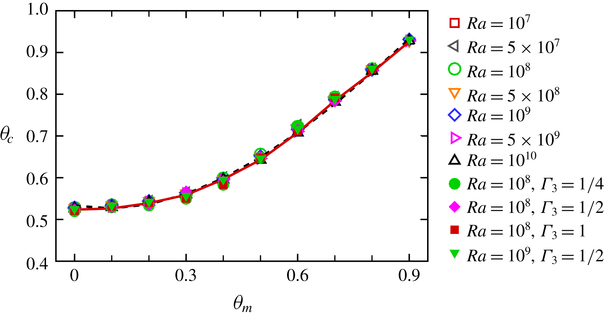
Reference Ahlers, Araujo, Funfschilling, Grossmann and Lohse2007) compared to that of the OB cases. Figure 6 shows
 $\unicode[STIX]{x1D703}_{c}$
as a function of
 $\unicode[STIX]{x1D703}_{m}$
for different
 $Ra$
for both 2-D cases and 3-D cases. An interesting finding is that all the data points can collapse well onto a single curve. As the thermal conductivity is assumed to be constant, the temperature gradients at the bottom and top walls should be equal, and the
 $Nu$
can be simply expressed as
 $Nu=-\unicode[STIX]{x2202}_{z}\langle \unicode[STIX]{x1D703}\rangle _{A,t}|_{z=1}=-\unicode[STIX]{x2202}_{z}\langle \unicode[STIX]{x1D703}\rangle _{A,t}|_{z=0}$
. Based on (3.1), one can obtain
 $$\begin{eqnarray}\displaystyle \unicode[STIX]{x1D703}_{c}=\frac{\unicode[STIX]{x1D706}_{t}^{\unicode[STIX]{x1D703}}}{\unicode[STIX]{x1D706}_{t}^{\unicode[STIX]{x1D703}}+\unicode[STIX]{x1D706}_{b}^{\unicode[STIX]{x1D703}}}. & & \displaystyle\end{eqnarray}$$
Thus
 $1/\unicode[STIX]{x1D703}_{c}=1/F_{\unicode[STIX]{x1D706}}+1$
. The solid red line in figure 6 shows a line segment of
 $\unicode[STIX]{x1D706}_{t}^{\unicode[STIX]{x1D703}}/(\unicode[STIX]{x1D706}_{t}^{\unicode[STIX]{x1D703}}+\unicode[STIX]{x1D706}_{b}^{\unicode[STIX]{x1D703}})$
as a function of
 $\unicode[STIX]{x1D703}_{m}$
calculated at different
 $\unicode[STIX]{x1D703}_{m}$
for
 $Ra=10^{10}$
, the data sets for different
 $Ra$
collapse well onto this curve. The dashed black curve is a polynomial fitting which is expressed as
 $\unicode[STIX]{x1D703}_{c}=0.530-0.133\unicode[STIX]{x1D703}_{m}+0.858\unicode[STIX]{x1D703}_{m}^{2}-0.237\unicode[STIX]{x1D703}_{m}^{3}$
, the data sets for different
 $Ra$
fall well onto this curve.
Centre temperature
 $\unicode[STIX]{x1D703}_{c}$
as a function of
 $\unicode[STIX]{x1D703}_{m}$
for different
 $Ra$
. Hollow symbols for 2-D simulations with
 $\unicode[STIX]{x1D6E4}=1$
, filled symbols for 3-D simulations. The solid line is line segment of
 $\unicode[STIX]{x1D706}_{t}^{\unicode[STIX]{x1D703}}/(\unicode[STIX]{x1D706}_{t}^{\unicode[STIX]{x1D703}}+\unicode[STIX]{x1D706}_{b}^{\unicode[STIX]{x1D703}})$
calculated at different
 $\unicode[STIX]{x1D703}_{m}$
for
 $Ra=10^{10}$
. The dashed line is a polynomial fitting which is expressed as
 $\unicode[STIX]{x1D703}_{c}=0.530-0.133\unicode[STIX]{x1D703}_{m}+0.858\unicode[STIX]{x1D703}_{m}^{2}-0.237\unicode[STIX]{x1D703}_{m}^{3}$
.

Absolute and normalized Nusselt numbers and Reynolds numbers as a function of
 $\unicode[STIX]{x1D703}_{m}$
for 2-D cases with different
 $Ra$
and fixed
 $\unicode[STIX]{x1D6E4}=1$
. (a) Absolute Nusselt number
 $Nu$
. (b) Normalized Nusselt number
 $Nu(\unicode[STIX]{x1D703}_{m})/Nu(0)$
, the red sold line denotes a line segment of
 $(\unicode[STIX]{x1D706}_{t}^{\unicode[STIX]{x1D703}}(0)+\unicode[STIX]{x1D706}_{b}^{\unicode[STIX]{x1D703}}(0))/(\unicode[STIX]{x1D706}_{t}^{\unicode[STIX]{x1D703}}(\unicode[STIX]{x1D703}_{m})+\unicode[STIX]{x1D706}_{b}^{\unicode[STIX]{x1D703}}(\unicode[STIX]{x1D703}_{m}))$
calculated for
 $Ra=10^{10}$
at different
 $\unicode[STIX]{x1D703}_{m}$
, the black dashed line denotes a polynomial fitting of
 $Nu(\unicode[STIX]{x1D703}_{m})/Nu(0)=0.992-0.170\unicode[STIX]{x1D703}_{m}-2.244\unicode[STIX]{x1D703}_{m}^{2}+1.397\unicode[STIX]{x1D703}_{m}^{3}$
. (c) Absolute Reynolds number
 $Re$
. (d) Normalized Reynolds number
 $Re(\unicode[STIX]{x1D703}_{m})/Re(0)$
, the black dashed line denotes a linear fitting of
 $Re(\unicode[STIX]{x1D703}_{m})/Re(0)=0.98-1.046\unicode[STIX]{x1D703}_{m}$
.

3.2 Nusselt number and Reynolds number
We now turn to the heat-transfer properties measured by the Nusselt number
 $Nu$
, and the flow intensity which can be expressed in terms of the Reynolds number
 $Re$
. The
 $Nu$
and
 $Re$
numbers are expressed as:
 $$\begin{eqnarray}\displaystyle Nu=\langle \sqrt{RaPr}u_{z}\unicode[STIX]{x1D703}-\unicode[STIX]{x2202}_{z}\unicode[STIX]{x1D703}\rangle _{A,t},\quad Re=\sqrt{Ra/Pr}U, & & \displaystyle\end{eqnarray}$$
where
 $\langle \rangle _{A,t}$
means average over any horizontal plane (3-D)/line (2-D) and time,
 $U=\sqrt{(\boldsymbol{u}\boldsymbol{\cdot }\boldsymbol{ u})_{y,z,t}}$
. The
 $Nu$
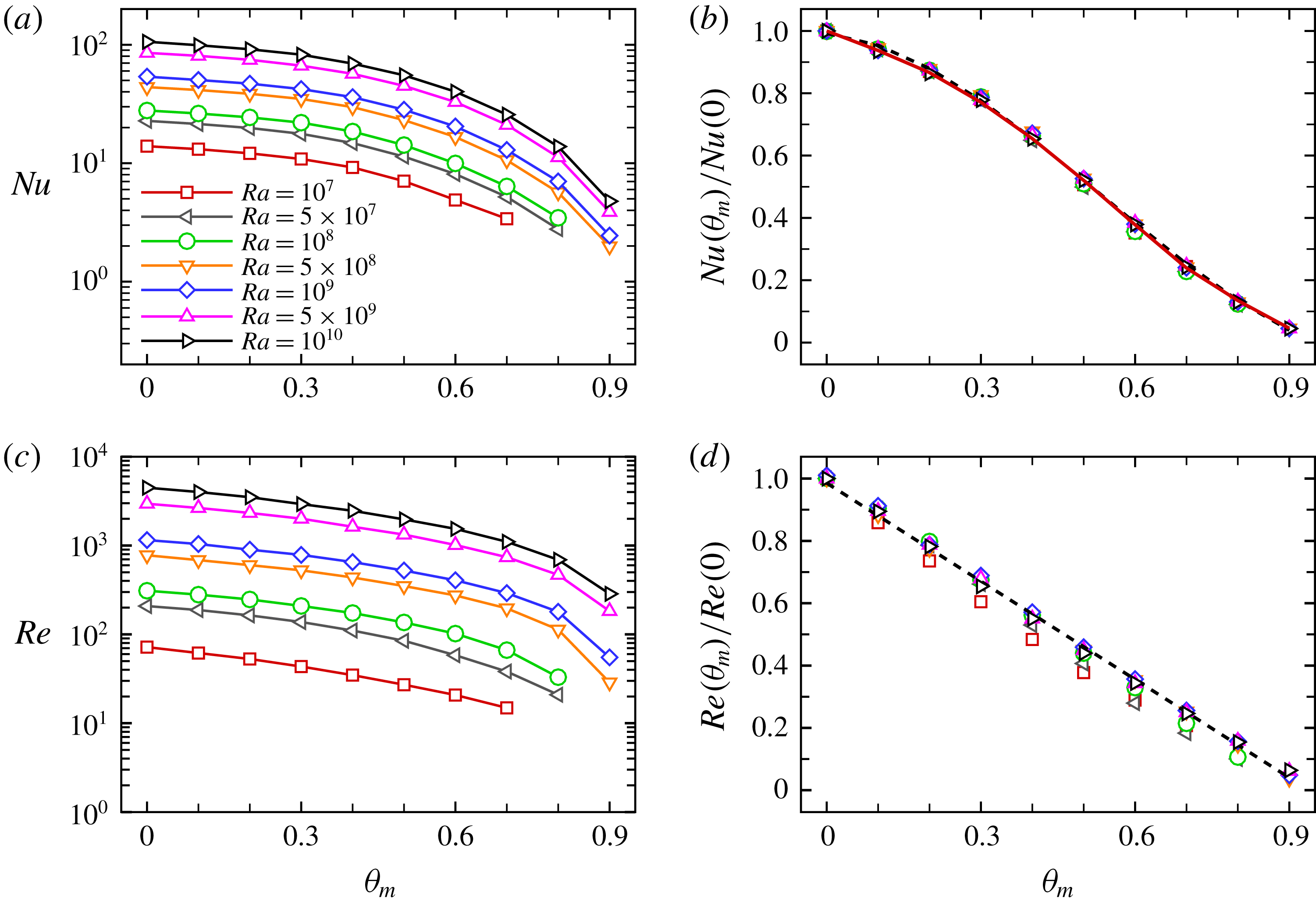
studied here is averaged over the bottom plate. In figure 7, we show the absolute and normalized
 $Nu$
and
 $Re$
as a function of
 $\unicode[STIX]{x1D703}_{m}$
for different
 $Ra$
for 2-D cases with
 $\unicode[STIX]{x1D6E4}=1$
. It is seen from figure 7(a) that
 $Nu$
drops monotonically with increasing
 $\unicode[STIX]{x1D703}_{m}$
. This is because with increasing
 $\unicode[STIX]{x1D703}_{m}$
, the stably stratified flow regimes gradually appear and grow near the top plate, where the flow is mainly dominated by thermal conduction. For the extreme limit
 $\unicode[STIX]{x1D703}_{m}=1$
, the flow should be totally within the conduction regime with
 $Nu=1$
. Figure 7(b) shows the normalized Nusselt number
 $Nu(\unicode[STIX]{x1D703}_{m})/Nu(0)$
as a function of
 $\unicode[STIX]{x1D703}_{m}$
for various
 $Ra$
. We can see that all data sets collapse well onto a single curve. From (3.1), one can obtain
 $Nu(\unicode[STIX]{x1D706}_{t}^{\unicode[STIX]{x1D703}}+\unicode[STIX]{x1D706}_{b}^{\unicode[STIX]{x1D703}})=1$
, and thus
 $$\begin{eqnarray}\displaystyle \frac{Nu(\unicode[STIX]{x1D703}_{m})}{Nu(0)}=\frac{\unicode[STIX]{x1D706}_{t}^{\unicode[STIX]{x1D703}}(0)+\unicode[STIX]{x1D706}_{b}^{\unicode[STIX]{x1D703}}(0)}{\unicode[STIX]{x1D706}_{t}^{\unicode[STIX]{x1D703}}(\unicode[STIX]{x1D703}_{m})+\unicode[STIX]{x1D706}_{b}^{\unicode[STIX]{x1D703}}(\unicode[STIX]{x1D703}_{m})}. & & \displaystyle\end{eqnarray}$$
We note that this relationship is analytically exact (see also Ahlers et al. (Reference Ahlers, Brown, Araujo, Funfschilling, Grossmann and Lohse2006), Horn et al. (Reference Horn, Shishkina and Wagner2013)). The red solid line in figure 7(b) shows a line segment of
 $(\unicode[STIX]{x1D706}_{t}^{\unicode[STIX]{x1D703}}(0)+\unicode[STIX]{x1D706}_{b}^{\unicode[STIX]{x1D703}}(0))/(\unicode[STIX]{x1D706}_{t}^{\unicode[STIX]{x1D703}}(\unicode[STIX]{x1D703}_{m})+\unicode[STIX]{x1D706}_{b}^{\unicode[STIX]{x1D703}}(\unicode[STIX]{x1D703}_{m}))$
as a function of
 $\unicode[STIX]{x1D703}_{m}$
calculated at different
 $\unicode[STIX]{x1D703}_{m}$
for
 $Ra=10^{10}$
. One can see that the data points for other
 $Ra$
values all nicely fall onto this curve. The black dashed curve is a polynomial fit denoted by
 $Nu(\unicode[STIX]{x1D703}_{m})/Nu(0)=0.992-0.170\unicode[STIX]{x1D703}_{m}-2.244\unicode[STIX]{x1D703}_{m}^{2}+1.397\unicode[STIX]{x1D703}_{m}^{3}$
, the data sets for different
 $Ra$
collapse well onto this fitted curve. Figure 7(c) shows the absolute
 $Re$
as a function of
 $\unicode[STIX]{x1D703}_{m}$
for different
 $Ra$
. It is seen that
 $Re$
also decreases monotonically with increasing
 $\unicode[STIX]{x1D703}_{m}$
. The reduction of
 $Re$
can be also qualitatively understood, from the point of view that the appearance of stably stratified flow structures weakens the fluid motion, and in turn the magnitude of
 $Re$
drops considerably. Figure 7(d) plots the normalized Reynolds number
 $Re(\unicode[STIX]{x1D703}_{m})/Re(0)$
as a function of
 $\unicode[STIX]{x1D703}_{m}$
. One can see that
 $Re(\unicode[STIX]{x1D703}_{m})/Re(0)$
roughly drops linearly with increasing
 $\unicode[STIX]{x1D703}_{m}$
, and the data sets can be described well by a linear fitting of
 $Re(\unicode[STIX]{x1D703}_{m})/Re(0)=0.980-1.046\unicode[STIX]{x1D703}_{m}$
. The curve is fitted for the
 $Ra=10^{10}$
data, and only the data sets for relatively low
 $Ra$
(i.e.
 $Ra=10^{7}$
and
 $5\times 10^{7}$
) show some deviations from this fitting.
Absolute and normalized Nusselt numbers and Reynolds numbers as a function of
 $\unicode[STIX]{x1D703}_{m}$
for different
 $\unicode[STIX]{x1D6E4}$
and fixed
 $Ra=10^{8}$
for 2-D simulations. (a) Absolute Nusselt number
 $Nu$
. (b) Normalized Nusselt number
 $Nu(\unicode[STIX]{x1D703}_{m})/Nu(0)$
. (c) Absolute Reynolds number
 $Re$
. (d) Normalized Reynolds number
 $Re(\unicode[STIX]{x1D703}_{m})/Re(0)$
. The dashed lines are the same as figure 7.

Absolute and normalized Nusselt numbers and Reynolds numbers as a function of
 $\unicode[STIX]{x1D703}_{m}$
for 3-D cases with different
 $\unicode[STIX]{x1D6E4}_{3}$
. (a) Absolute Nusselt number
 $Nu$
. (b) Normalized Nusselt number
 $Nu(\unicode[STIX]{x1D703}_{m})/Nu(0)$
. (c) Absolute Reynolds number
 $Re$
. (d) Normalized Reynolds number
 $Re(\unicode[STIX]{x1D703}_{m})/Re(0)$
. The dashed lines are the same as figure 7.

We then investigate the aspect ratio
 $\unicode[STIX]{x1D6E4}$
dependence of
 $Nu$
and
 $Re$
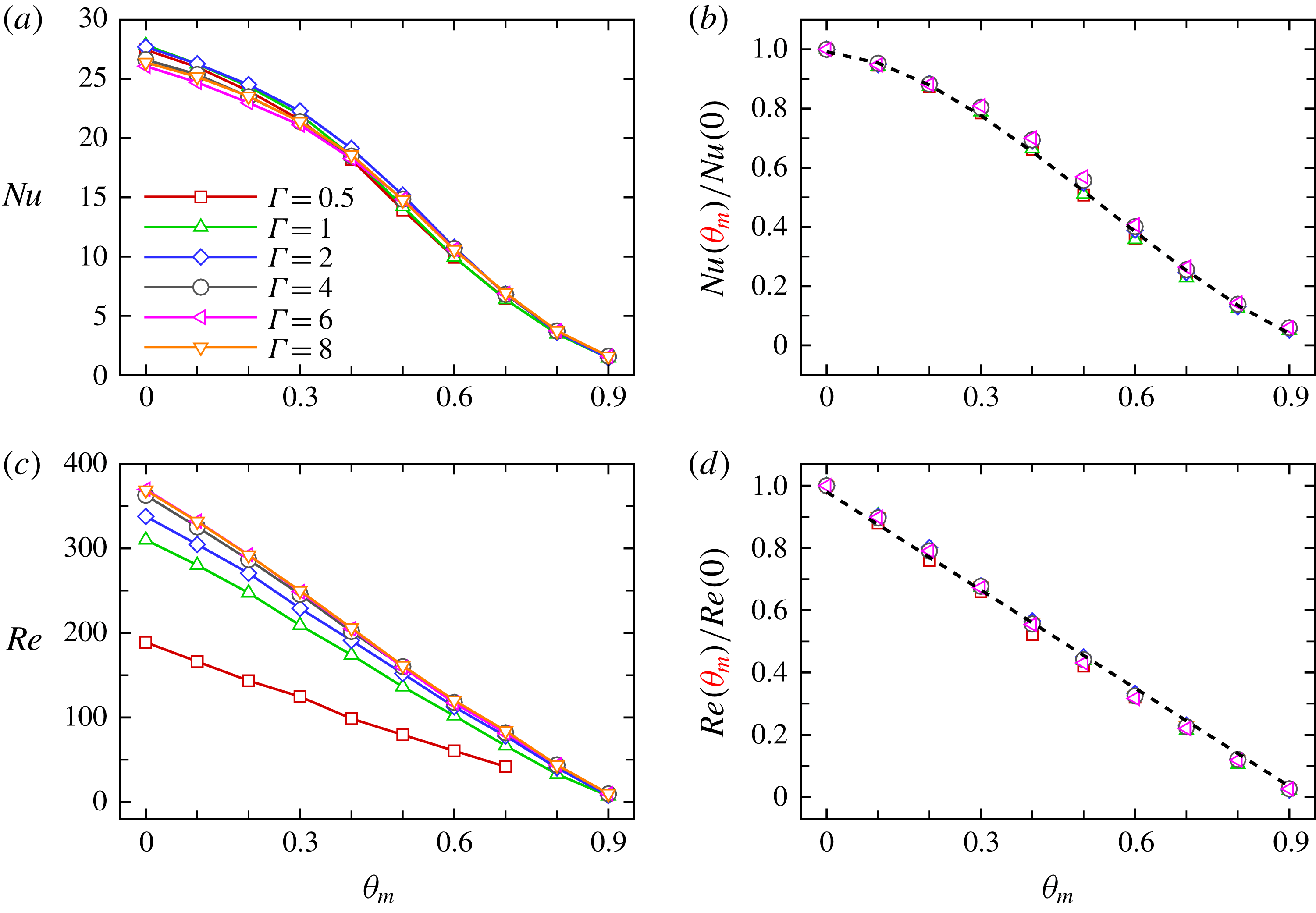
. Figure 8 shows the absolute and normalized
 $Nu$
and
 $Re$
as a function of
 $\unicode[STIX]{x1D703}_{m}$
for different
 $\unicode[STIX]{x1D6E4}$
and fixed
 $Ra=10^{8}$
for 2-D simulations. For large
 $\unicode[STIX]{x1D6E4}$
, it was already found that multiple states with different numbers of convection rolls may exist (Wang et al.
Reference Wang, Wan, Yan and Sun2018a
), and this will lead to different heat-transfer properties. To avoid such possible multiple states from complicating the present problem, we gradually increase
 $\unicode[STIX]{x1D703}_{m}$
using the flow field for smaller
 $\unicode[STIX]{x1D703}_{m}$
as initial conditions. The
 $Nu$
still reduces monotonically with increasing
 $\unicode[STIX]{x1D703}_{m}$
and again the normalized Nusselt numbers for different
 $\unicode[STIX]{x1D6E4}$
collapse well on top of each other, implying the insensitivity of this dependence on
 $\unicode[STIX]{x1D6E4}$
. From figure 8(c), one sees that for all considered
 $\unicode[STIX]{x1D6E4}$
,
 $Re$
decreases linearly with increasing
 $\unicode[STIX]{x1D703}_{m}$
, and drops with decreasing
 $\unicode[STIX]{x1D6E4}$
due to the geometric confinement of the side walls. The normalized Reynolds number
 $Re(\unicode[STIX]{x1D703}_{m})/Re(0)$
for different
 $\unicode[STIX]{x1D6E4}$
also collapse well onto the fitted curve
 $Re(\unicode[STIX]{x1D703}_{m})/Re(0)=0.980-1.046\unicode[STIX]{x1D703}_{m}$
as shown in figure 8(d), suggesting an aspect ratio insensitive feature.
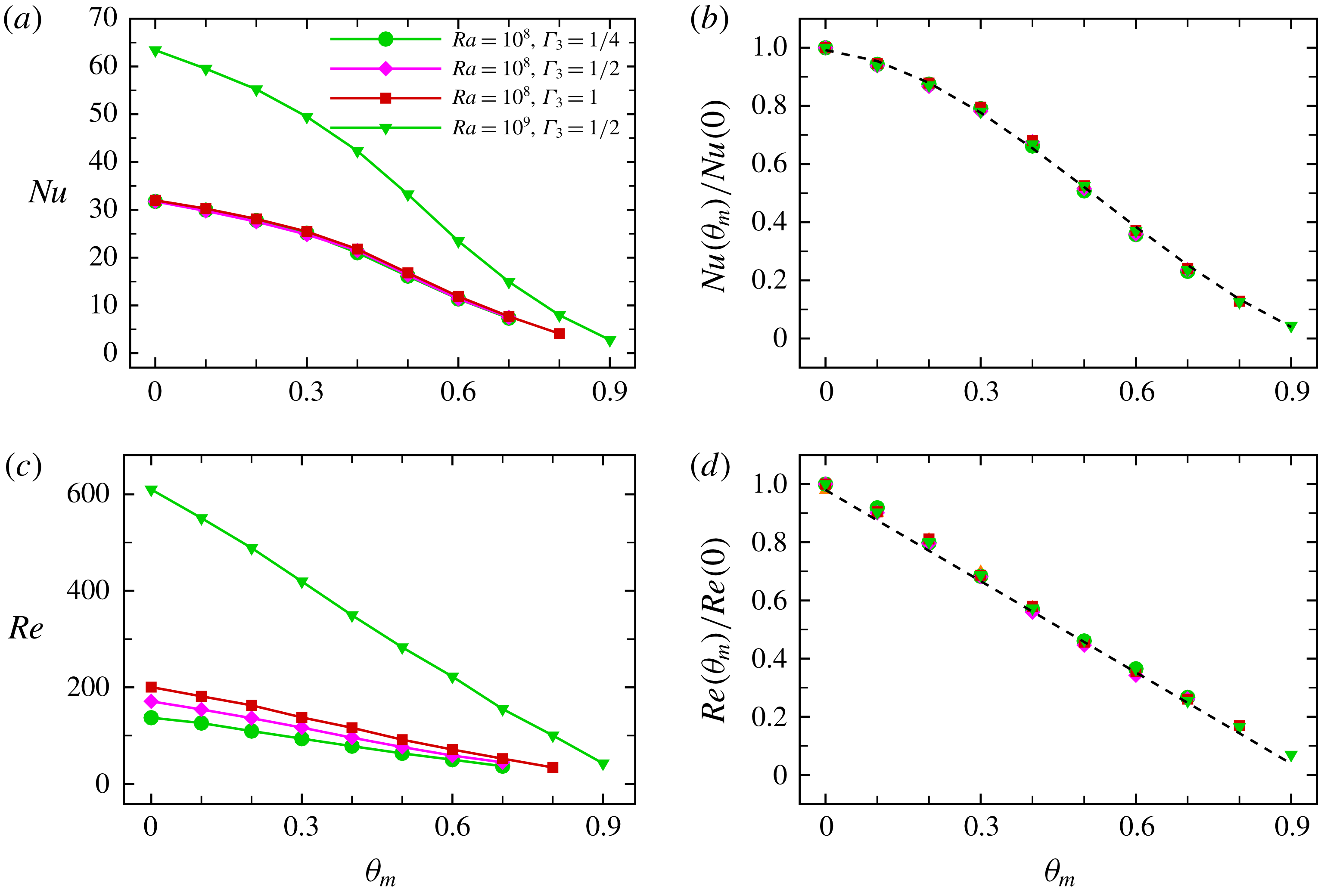
We also show the 3-D results in figure 9 in order to find whether the universal behaviour for normalized Nusselt number and Reynolds number found in two dimensions can be extended to 3-D cases. For
 $Ra=10^{8}$
, we only consider the cases with
 $\unicode[STIX]{x1D6E4}_{3}\geqslant 1/4$
. For smaller
 $\unicode[STIX]{x1D6E4}_{3}$
, where the flow is in the confined (Huang et al.
Reference Huang, Kaczorowski, Ni and Xia2013; Chong et al.
Reference Chong, Huang, Kaczorowski and Xia2015, Reference Chong, Yang, Huang, Zhong, Stevens, Verzicco, Lohse and Xia2017, Reference Chong, Wagner, Kaczorowski, Shishkina and Xia2018) or severely confined regime (Chong & Xia Reference Chong and Xia2016), the flow is laminar for a wide range of
 $\unicode[STIX]{x1D703}_{m}$
, which is not the focus of the present study. We can clearly see in figure 9(a) that the absolute
 $Nu$
is less influenced by
 $\unicode[STIX]{x1D6E4}_{3}$
for all considered
 $\unicode[STIX]{x1D703}_{m}$
, despite the fact that the flow strength is weakened when reducing
 $\unicode[STIX]{x1D6E4}_{3}$
as illustrated in figure 9(c). After normalization, the data for both
 $Nu$
and
 $Re$
again fall onto a single curve as seen in figures 9(b) and 9(d). Thus, we can conclude that the universal behaviour for normalized
 $Nu$
and
 $Re$
can also be found in 3-D configurations.
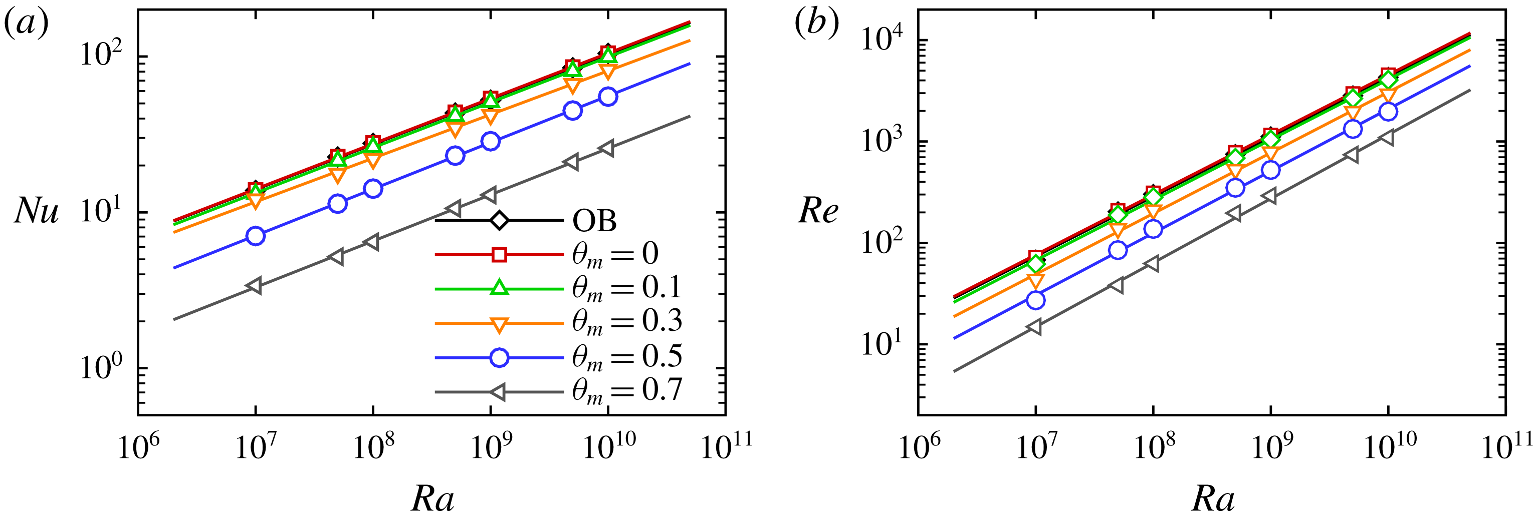
(a) Nusselt number
 $Nu$
and (b) Reynolds number
 $Re$
as a function of
 $Ra$
for different
 $\unicode[STIX]{x1D703}_{m}$
for 2-D simulations.

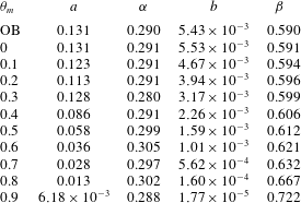
The coefficients of the fitted scalings
 $Nu\sim aRa^{\unicode[STIX]{x1D6FC}}$
and
 $Re\sim bRa^{\unicode[STIX]{x1D6FD}}$
.

We finally discuss the scalings of the
 $Nu$
and
 $Re$
versus
 $Ra$
for different
 $\unicode[STIX]{x1D703}_{m}$
. As mentioned above
 $Nu(\unicode[STIX]{x1D703}_{m})/Nu(0)$
and
 $Re(\unicode[STIX]{x1D703}_{m})/Re(0)$
both have universal relationships with
 $\unicode[STIX]{x1D703}_{m}$
which are independent of
 $Ra$
, and thus the scaling exponents of
 $Nu\sim aRa^{\unicode[STIX]{x1D6FC}}$
and
 $Re\sim bRa^{\unicode[STIX]{x1D6FD}}$
for different
 $\unicode[STIX]{x1D703}_{m}$
should also be expected to be independent of
 $\unicode[STIX]{x1D703}_{m}$
. Figure 10(a) shows a log–log plot of
 $Nu$
versus
 $Ra$
for the OB and penetrative cases with different
 $\unicode[STIX]{x1D703}_{m}$
for 2-D simulations. Detailed exponents and prefactors for all the
 $\unicode[STIX]{x1D703}_{m}$
considered in this work are listed in table 1. For the OB case, the scaling exponent 0.29 is quite close to those obtained in the previous 2-D studies. For example, Johnston & Doering (Reference Johnston and Doering2009) obtained 0.285 for periodic cells with
 $Pr=1$
, Huang & Zhou (Reference Huang and Zhou2013) obtained 0.29 for
 $Pr=10$
for no-slip side walls similar to the present study. Zhang, Zhou & Sun (Reference Zhang, Zhou and Sun2017) obtained
 $0.3\pm 0.02$
for
 $Pr=0.71$
and 5.3 also for no-slip side walls. For penetrative cases all the exponents vary between 0.28 and 0.3 for different
 $\unicode[STIX]{x1D703}_{m}$
, i.e. the scaling exponent does not change much for the penetrative cases. Figure 10(b) shows a log–log plot of
 $Re$
versus
 $Ra$
for 2-D simulations. For the OB case, the scaling exponent 0.59 is also quite close to previous 2-D studies (0.62 for
 $Pr=4.3$
(Sugiyama et al.
Reference Sugiyama, Calzavarini, Grossmann and Lohse2009) and 0.6 for
 $Pr=0.71$
and 5.3 (Zhang et al.
Reference Zhang, Zhou and Sun2017)). For penetrative cases, as listed in table 1, one can see that the scaling exponent for
 $Re$
only deviates from the OB case for large
 $\unicode[STIX]{x1D703}_{m}$
close to 0.9. According to the data listed in table 1, one may come to the conclusion that the scaling exponents are almost unchanged for the penetrative cases for not too large
 $\unicode[STIX]{x1D703}_{m}$
. It is interesting that the scaling exponents are so robust to this density maximum effect despite of the remarkable change of the flow organization as mentioned before.
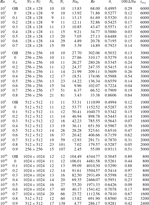
Two-dimensional simulation parameters. The columns from left to right indicate Rayleigh number
 $Ra$
, density inversion parameter
 $\unicode[STIX]{x1D703}_{m}$
(OB cases are also included for comparison), grid resolution, number of grid points in the bottom (
 $N_{b}$
) and top (
 $N_{t}$
) thermal boundary layers, Nusselt number at the bottom plate
 $Nu_{b}$
, Reynolds number
 $Re$
, centre temperature
 $\unicode[STIX]{x1D703}_{c}$
, the difference between Nusselt number at the bottom and top plates (
 $\unicode[STIX]{x0394}Nu=|Nu_{b}-Nu_{t}|/Nu_{b}$
) and the averaging time for the simulations
 $t_{avg}$
. Note that not all the 2-D simulations in this work are listed in this table.

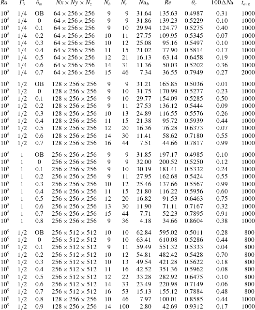
Three-dimensional simulation parameters. The columns from left to right indicate Rayleigh number
 $Ra$
, density inversion parameter
 $\unicode[STIX]{x1D703}_{m}$
(OB cases are also included for comparison), grid resolution, number of grid points in the bottom (
 $N_{b}$
) and top (
 $N_{t}$
) thermal boundary layers, Nusselt number at the bottom plate
 $Nu_{b}$
, Reynolds number
 $Re$
, centre temperature
 $\unicode[STIX]{x1D703}_{c}$
, the difference between Nusselt number at the bottom and top plates (
 $\unicode[STIX]{x0394}Nu=|Nu_{b}-Nu_{t}|/Nu_{b}$
) and the averaging time for the simulations
 $t_{avg}$
.

4 Conclusion
In summary, we have studied penetrative turbulent RBC of water near
 $4\,^{\circ }\text{C}$
using 2-D and 3-D DNS. In the present system, the flow dynamics and heat transport highly depend on an important parameter, i.e. the density inversion parameter
 $\unicode[STIX]{x1D703}_{m}$
. Several universal properties are identified and are found to hold over a wide range of parameters for both two and three dimensions. The ratio of the top and bottom thermal BL thicknesses
 $F_{\unicode[STIX]{x1D706}}$
increases with increasing
 $\unicode[STIX]{x1D703}_{m}$
, and the relationship is found to be independent of
 $Ra$
. Similar to the previous studies for NOB convection caused by large temperature differences, the centre temperature
 $\unicode[STIX]{x1D703}_{c}$
is particularly investigated;
 $\unicode[STIX]{x1D703}_{c}$
is found to be increased compared to that of the OB cases. As
 $\unicode[STIX]{x1D703}_{c}$
is related to
 $F_{\unicode[STIX]{x1D706}}$
with
 $1/\unicode[STIX]{x1D703}_{c}=1/F_{\unicode[STIX]{x1D706}}+1$
,
 $\unicode[STIX]{x1D703}_{c}$
also has a universal relationship with
 $\unicode[STIX]{x1D703}_{m}$
which is valid for both 2-D and 3-D cases. With increasing
 $\unicode[STIX]{x1D703}_{m}$
, both the heat transfer and the flow intensity are substantially weakened. The normalized Nusselt number
 $Nu(\unicode[STIX]{x1D703}_{m})/Nu(0)$
and Reynolds number
 $Re(\unicode[STIX]{x1D703}_{m})/Re(0)$
also have a universal dependence on
 $\unicode[STIX]{x1D703}_{m}$
which seems to be independent of both
 $Ra$
and the aspect ratio
 $\unicode[STIX]{x1D6E4}$
. Finally, the scaling laws of
 $Nu$
and
 $Re$
versus
 $Ra$
are investigated. It is interesting to find that the scaling exponents of
 $Nu\sim Ra^{\unicode[STIX]{x1D6FC}}$
and
 $Re\sim Ra^{\unicode[STIX]{x1D6FD}}$
, i.e.
 $\unicode[STIX]{x1D6FC}\approx 0.29$
and
 $\unicode[STIX]{x1D6FD}\approx 0.59$
, are insensitive to
 $\unicode[STIX]{x1D703}_{m}$
, despite the drastic changes in the flow organization.
Acknowledgements
We wish to thank K. Leong Chong for helpful discussions. This work is supported by National Natural Science Foundation of China under grants (11572314, 11772323, 11621202 and 11825204), and the Fundamental Research Funds for the Central Universities.
Appendix. Simulation details
The details of the main 2-D simulations are listed in table 2 and the 3-D simulations in table 3. In order not to make the tables too long, we only list some of the main cases for 2-D simulations. It can be seen that the differences between
 $Nu$
at the hot and cold plates are generally within 1 %.