1. Introduction
Localised turbulence in subcritical transition of pipe and Couette flows has been shown to be transient in nature, i.e. the turbulence will decay at a finite time with a characteristic mean lifetime at a given Reynolds number,
 $Re$
, and the decay was shown to be stochastic and memoryless (Hof et al. Reference Hof, Westerweel, Schneider and Eckhardt2006; Peixinho & Mullin Reference Peixinho and Mullin2006; Willis & Kerswell Reference Willis and Kerswell2007; Avila et al. Reference Avila, Willis and Hof2010; Borrero-Echeverry et al. Reference Borrero-Echeverry, Schatz and Tagg2010; Shi et al. Reference Shi, Avila and Hof2013). This memoryless transient nature is essential for the analogy between transition to turbulence and directed percolation phase transition (DP) (Hinrichsen Reference Hinrichsen2000; Barkley Reference Barkley2016; Lemoult et al. Reference Lemoult, Shi, Avila, Jalikop, Avila and Hof2016; Shih et al. Reference Shih, Hsieh and Goldenfeld2016; Chantry et al. Reference Chantry, Tuckerman and Barkley2017; Hof Reference Hof2022; Klotz et al. Reference Klotz, Lemoult, Avila and Hof2022; Lemoult et al. Reference Lemoult, Mukund, Shih, Linga, Mathiesen, Goldenfeld and Hof2024), and has been expected to be universal to localised turbulence in all basic shear flows. However, the temporal characteristics of localised turbulence in channel flow remain unclear and debated to date.
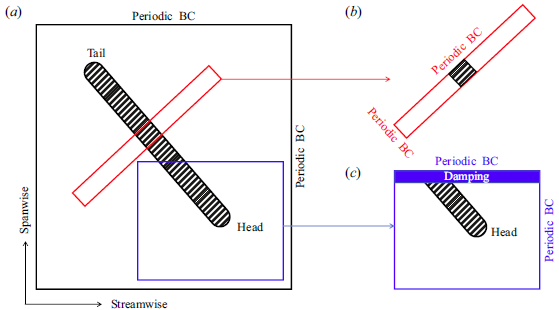
At transitional Reynolds numbers, localised turbulence in channel flow can organise itself into a banded structure obliquely oriented about the streamwise direction (Tsukahara et al. Reference Tsukahara, Seki, Kawamura and Tochio2005; Tuckerman et al. Reference Tuckerman, Kreilos, Shrobsdorff, Schneider and Gibson2014). If the turbulent band is strongly constrained by a narrow periodic dimension along the band (see figure 1 b), effectively resulting in an infinite periodic band (referred to as the quasi-one-dimensional band hereafter), similar memoryless decay was found (Gomé et al. Reference Gomé, Tuckerman and Barkley2020, Reference Gomé, Tuckerman and Barkley2022). However, in a sufficiently large flow domain, a turbulent band becomes fully localised (i.e. with a finite length) by forming an upstream end and a downstream end (Xiong et al. Reference Xiong, Tao, Chen and Brandt2015; Kanazawa Reference Kanazawa2018; Tao et al. Reference Tao, Eckhardt and Xiong2018; Paranjape Reference Paranjape2019; Shimizu & Manneville Reference Shimizu and Manneville2019; Kashyap et al. Reference Kashyap, Duguet and Dauchot2020; Song & Xiao Reference Song and Xiao2020; Xiao & Song Reference Xiao and Song2020a , Reference Xiao and Song b ; Mukund et al. Reference Mukund, Paranjape, Sitte and Hof2021; Marensi et al. Reference Marensi, Yalniz and Hof2023), see figure 1(a) for a sketch. The dynamics at the two ends are asymmetric with turbulence being generated continuously at the downstream end (referred to as head hereafter) and decaying or chipping intermittently at the upstream end (referred to as tail hereafter). The generation of turbulence at the head is through nearly periodic streak and vortex generation (Kanazawa Reference Kanazawa2018; Paranjape Reference Paranjape2019; Xiao & Song Reference Xiao and Song2020a ; Mukund et al. Reference Mukund, Paranjape, Sitte and Hof2021; Marensi et al. Reference Marensi, Yalniz and Hof2023), which was attributed to either an inflectional crossflow instability associated with the local meanflow (Song & Xiao Reference Song and Xiao2020; Xiao & Song Reference Xiao and Song2020a , Reference Xiao and Songb ) or a localised exact coherent structure (Kanazawa Reference Kanazawa2018). This dynamics at the head was shown to be essential for the growth and self-sustaining mechanism of the whole band (Song & Xiao Reference Song and Xiao2020; Mukund et al. Reference Mukund, Paranjape, Sitte and Hof2021; Wu & Song Reference Wu and Song2022; Marensi et al. Reference Marensi, Yalniz and Hof2023) and contributes to the tilt angle selection for the band as well (Zhang & Tao Reference Zhang and Tao2023).
After being seeded, a short band will grow in length
 $l$
initially due to the faster turbulence generation at the head. However, the chipping and decay of turbulence at the tail eventually will limit
 $l$
and keep it finite, which is
 $O(100)$
channel heights at
 $Re\simeq 660$
and increases with
 $Re$
(Kanazawa Reference Kanazawa2018). In this paper,
 $Re$
is based on the half-channel height
 $h$
(will be used as the length unit hereafter), the centreline velocity of the basic laminar flow and the fluid viscosity. Besides the length scale, the time scale of a turbulent band is also large. Above
 $Re\simeq 660$
, it can evolve for approximately
 $10^4$
time units without a sign of decay (Kanazawa Reference Kanazawa2018; Tao et al. Reference Tao, Eckhardt and Xiong2018; Paranjape Reference Paranjape2019; Xiao & Song Reference Xiao and Song2020a
). These two factors require large flow domain and observation time for clarifying the temporal behaviour of a band in either experiments or direct numerical simulations (DNS).
Some studies, from different perspectives, proposed that a turbulent band becomes sustained above a critical
 $Re$
. Kanazawa (Reference Kanazawa2018) proposed
 $Re\simeq 660$
because the exact coherent structure they identified at the head appears at
 $Re\simeq 660$
and is stable. Tao et al. (Reference Tao, Eckhardt and Xiong2018) proposed that a band can become sustained at
 $Re\simeq 700$
via breaking and reconnecting in a computation box with a specific aspect ratio, based on an observation time of
 $10^4$
. Paranjape (Reference Paranjape2019) proposed
 $Re\simeq 650$
because band growth outweighs shrinking on average at higher
 $Re$
whereas it is the opposite otherwise. The observation time in their experiment was
 $O(10^3)$
, which is the largest reported for experiments to our knowledge. Shimizu & Manneville (Reference Shimizu and Manneville2019) proposed
 $Re\approx 700$
by DNS based on an observation time of
 $1.5\times 10^5$
, but the conclusion was drawn for the global turbulent state in a large periodic flow domain rather than for a single turbulent band. In comparison, in the quasi-one-dimensional case, the band is of a lifetime of just
 $O(10^2)$
at
 $Re\simeq 700$
and remains transient up to
 $Re\simeq 1000$
(Gomé et al. Reference Gomé, Tuckerman and Barkley2020), indicating that the full localisation makes a significant difference. If a band indeed becomes sustained at a critical
 $Re$
, it would lead to a completely different transition route to turbulence compared with pipe and Couette flows.
Due to the large length and time scales of fully developed bands, statistical investigation was lacking in previous DNS studies where conclusions were made based on a single or only a few realisations, while it was difficult to achieve long observation times in experiments. To manage a statistical study with sufficiently long observation times, Xu & Song (Reference Xu and Song2022) considered a moderately constrained band by keeping the head while damping the tail (see figure 1
c). This technique allows the authors to fix and control
 $l$
so as to prepare well-controlled initial conditions and reduce costs. In the parameter regime of
 $l\leqslant 70$
and
 $Re\leqslant 675$
, the authors observed memoryless decay and the length-dependent nature of the mean lifetime. The lifetime increases quickly with both increasing
 $l$
and
 $Re$
but remains finite in this parameter regime. For example, the mean lifetime is already larger than
 $10^4$
for
 $Re=655$
with
 $l\approx 70$
and
 $Re=665$
with
 $l\approx 54$
. Decay was also observed in a single run at
 $Re=685$
with
 $l\approx 38$
(survival time
 $O(10^5)$
) and
 $Re=660$
with
 $l\approx 110$
(survival time
 $O(10^4)$
), but statistical studies were not carried out because of the large lifetime. The authors conjectured that a fully developed band is transient by nature and the discrepancies between the reported critical
 $Re$
values for sustained turbulence are possibly attributed to the different observation times and lack of statistics. However, the band lengths considered in Xu & Song (Reference Xu and Song2022) were much shorter than the fully developed ones and were artificially fixed, i.e. the artificial constraint was still rather strong; it is unclear whether a fully developed band with a naturally varying length, due to the intermittent chipping and decay of the turbulence at the tail, is still transient and memoryless. The aim of this paper is to clarify this problem by considering fully developed bands.
Sketches of the flow domains for studying turbulent band in channel flow in numerical simulations. The shaded area represents turbulent region and blank area represents laminar region. (a) The normal computational box with one edge parallel to the streamwise direction. (b) The tilted narrow computational box with the short edge parallel to the band. (c) The normal box with a small damping region, both of which co-move with the head of the band. Periodic boundary conditions (BCs) are imposed as indicated in the figure.

2. Methods
The same numerical method as described in Xu & Song (Reference Xu and Song2022) is used here. Given the low
 $Re$
, 56 Chebyshev grid points and a finite-difference differentiation with a 9-point stencil are used in the wall-normal direction (
 $y$
). Periodic BCs and Fourier spectral methods are used in the streamwise (
 $x$
) and spanwise (
 $z$
) directions, and the grid sizes are
 $h/\Delta x=4.6$
and
 $h/\Delta z=5.5$
in these two directions, respectively. This resolution is comparable to those used in the literature for studying turbulent band at slightly higher Reynolds numbers (Kanazawa Reference Kanazawa2018; Tao et al. Reference Tao, Eckhardt and Xiong2018; Shimizu & Manneville Reference Shimizu and Manneville2019; Kashyap et al. Reference Kashyap, Duguet and Dauchot2020; Marensi et al. Reference Marensi, Yalniz and Hof2023). The time-step size is fixed at
 $\Delta t=0.025$
. This setting assures a decrease of nearly four orders of magnitude in the spectra of the maximum amplitude of the Fourier coefficient of the velocities in the whole domain. A constant mass flux is imposed by dynamically adjusting the driving pressure gradient. More details about the numerical method can be found in Xiao & Song (Reference Xiao and Song2020a
) and Xu & Song (Reference Xu and Song2022).
Following Xu & Song (Reference Xu and Song2022), a computation setting as sketched in figure 1(c) is used in this study. The computation box moves, keeping the head of the band fixed at approximately
 $z=30$
. An average speed of the head was measured every 25 time units and then the speed of the computation box was adjusted accordingly. The streamwise and spanwise sizes are
 $l_x=150$
and
 $l_z=140$
, respectively, the damping region is
 $130\lt z\lt 140$
and the head is located at
 $z=30$
, see figure 2(a). Therefore, the distance between the head and the damping region is
 $L_z=100$
, which sets the maximum of the spanwise length of a band. Correspondingly, the maximum band length is
 $l\approx 160$
given that the tilt angle of a band about the streamwise direction is approximately
 $40^\circ$
in the
 $Re$
regime considered here (Tao et al. Reference Tao, Eckhardt and Xiong2018; Paranjape Reference Paranjape2019; Xiao & Song Reference Xiao and Song2020b
; Zhang & Tao Reference Zhang and Tao2023). Reynolds numbers
 $640$
and
 $630$
are chosen for this study.
The computational box (a) and the distance between the damping region and the tail of a turbulent band (b). In (a), wall-normal velocity fluctuation
 $u_y$
is plotted in the
 $x{-}z$
cutplane at
 $y=-0.5$
. Red colour represents positive and blue represents negative values. The head of the band is fixed at
 $z=30$
and the damping region is between
 $z=130$
and 140. The spanwise distance between the tail and the damping region is denoted as
 $d$
. Panel (b) shows the time series of the distance
 $d$
for a run at
 $Re=640$
. The blue curve is based on
 $u_y$
and the red curve is based on
 $u_x$
. Panel (a) is taken at
 $t=2500$
from the time series shown in (b).

Figure 2(b) shows the spanwise distance
 $d$
between the tail of a rather long-lived band and the damping region at
 $Re=640$
. It can be seen that
 $d$
is considerably larger than zero in a large portion of the time, especially when
 $d$
is measured using the wall-normal velocity fluctuation
 $u_y$
. This indicates that, often, the tail of this band does not reach the damping region, i.e. the computation setting shown in figure 2(a) allows to account for the factor of length variation. The velocity streaks at the tail can reach the damping region more often; see the time windows in which
 $d\approx 0$
based on the streamwise velocity fluctuation
 $u_x$
in figure 2(b). Therefore, the damping region is necessary for damping out these streaks, or a segment of band chipped off so that the head will not be affected by them due to the periodic BC. It should be noted that, in a larger domain without the damping, a band may temporarily get considerably longer than the limit set by our setting (see supplementary movie 1 available at https://doi.org/10.1017/jfm.2025.299). Nevertheless, we will show more quantitatively later in § 3 that this setting allows the band to fully develop in terms of the mean lifetime.
The spanwise speed of the head
 $|c_z|$
(a, c) and the kinetic energy of turbulent velocity fluctuations
 $KE$
(b, d) of a few runs at
 $Re=630$
(a, b) and 640 (c, d). The same computation setting as shown in figure 2(a) is used. The horizontal straight line in (a, c) denotes
 $c_z=0.07$
which can be used as the threshold for determining a decay event.

We use the Reynolds-number-quenching technique to perturb the flow. Specifically, velocity snapshots from long-lived turbulent bands simulated in the same computation setting at
 $Re=645$
, 650 and 660 are used as the initial conditions. This assures that all initial conditions are highly similar. The head has nearly constant streamwise and spanwise travelling speeds during the lifetime of a band, but will slow down when the band starts to decay (Paranjape Reference Paranjape2019; Mukund et al. Reference Mukund, Paranjape, Sitte and Hof2021; Xu & Song Reference Xu and Song2022); see Appendix A for more details about the decay process. Therefore, spanwise speed of the head
 $|c_z|$
is a candidate for the diagnosis of a decay event, see figure 3(a, c). Note that this speed can be negative or positive depending on the orientation of the band. The orientation we chose actually gives a negative speed, i.e. the head moves to the negative
 $z$
direction. However, we will refer to
 $|c_z|$
as the spanwise speed in the following. The traditional diagnosis, the total kinetic energy of the turbulent fluctuations (
 $KE$
), does not serve as well as
 $|c_z|$
at
 $Re=630$
when the lifetime is short (see figure 3
b). Firstly, the decrease of
 $KE$
is less sharp. Secondly, the decrease of
 $|c_z|$
and
 $KE$
are often not synchronised, i.e.
 $KE$
may have not started decreasing when
 $|c_z|$
has already decreased significantly; see the bold green, magenta and black curves in figure 3(a, b). If the decay is to be diagnosed by setting a sufficiently low threshold in
 $KE$
, this time delay could significantly affect the measured lifetime when the lifetime itself is short. Thirdly, a longer decaying band may even have larger kinetic energy than a shorter sustaining band. Therefore,
 $|c_z|$
is chosen as the diagnosis of the decay of a band. Nevertheless,
 $KE$
may work equally well for
 $Re=640$
at which the lifetime is much larger than the above-mentioned time delay (see figure 3
d).
Figure 3 indicates a stochastic behaviour of the decay and sensitive dependence on the initial conditions. Following the method of Avila et al. (Reference Avila, Willis and Hof2010), for a stochastic decay process, the survival rate is defined as
 $S(t)=P\{\mathrm {survival\,time}\geqslant t\}$
and the escape rate can be defined as
 $\kappa =- {1}/{S(t)} {\mathrm {d}S(t)}/{\mathrm {d}t}$
. For a process that only becomes memoryless after a time instance
 $t_0$
, there would be
 $\kappa =\mathrm {const.}$
and consequently
 $S(t)\propto \exp (-\kappa (t-t_0))$
for
 $t\gt t_0$
. Then
 $S(t)$
would correspond to the distribution function of an exponential distribution, and the mean (mathematical expectation) lifetime of the process is given by
 $\tau =1/\kappa$
. In a random experiment,
 $\tau$
can be estimated with the sample mean of the decay time if the population obeys an exponential distribution. The estimation of
 $\kappa$
will simply be taken as the inverse of the estimated
 $\tau$
.
However,
 $t_0$
is not known a priori. In practice, selecting a value arbitrarily, the subsample in which the turbulence survives longer than
 $t_0$
will be used for the estimation. Then,
 $t_0$
is gradually increased and the same procedure is repeated. A
 $t_0$
-independent estimation of
 $\tau$
(also
 $\kappa$
) is supposed to be obtained if the entire subsample has started obeying an exponential distribution. In this case, it is considered that the decay has become memoryless and the turbulent trajectory has entered a chaotic saddle (Faisst & Eckhardt Reference Faisst and Eckhardt2004; Schneider & Eckhardt Reference Schneider and Eckhardt2008; Avila et al. Reference Avila, Willis and Hof2010). In the following, we show the statistics where the estimations are still denoted as
 $\tau$
and
 $\kappa$
.
3. Results
Statistics for
 $Re=640$
are shown in figure 4. It requires setting a proper threshold in
 $|c_z|$
below which the turbulent trajectory is considered to have escaped from the saddle. As the speed
 $|c_z|$
mainly fluctuates between 0.08 and 0.1 during the lifetime (figure 3
c),
 $c_z=0.065$
is used as the threshold for detecting a decay event. Because the survival time is several thousand and the drop in
 $|c_z|$
is sharp during the decay on this time scale, as shown in figure 3(c), different thresholds, say 0.07 and 0.06, do not make a significant difference in our tests.
The damping with
 $L_z=100$
still constrains the band and could still affect the lifetime. Due to the chaotic nature of turbulence, it certainly will affect the lifetime of an individual band, but here we show the saturation of the mean lifetime with respect to
 $L_z$
. Beside
 $L_z=100$
, two lower values of
 $L_z=80$
and 60 are considered to realise two smaller band lengths (recall the definition of
 $L_z$
in figure 2
a). Figure 4(a) shows the survival rate for the three cases. For the shortest case
 $L_z=60$
, corresponding to the band length of
 $l\approx 93$
, the slope of the tail of
 $S$
is significantly larger than the other two cases, indicating a shorter lifetime, in agreement with the size-dependence of the lifetime reported by Xu & Song (Reference Xu and Song2022). It is difficult to conclude whether or not there is a plateau region in
 $\kappa$
with the sample considered. A plateau might be forming after
 $t\approx 1800$
but the data points are rather scattered (see figure 4
b). Nevertheless, straightness can be observed in the tail of the
 $S{-}t$
plot as shown in figure 4(a) and the inset. Using
 $t_0=1825$
, which gives a subsample size of
 $N_s=58$
, we get
 $\tau =436\pm 112$
with
 $95$
% confidence (
 $\pm 1.96/\sqrt {N_s}$
times the sample mean). The exponentials
 $ae^{-\kappa (t-t_0)}$
with these estimations, where
 $a=S(t_0)$
, seem to fit the tail of
 $S$
reasonably well (see figure 4
a and the inset). On the other hand, the slopes of the tails of the other two cases seem to be parallel straight lines in the semilog-scale plot, suggesting exponentially distributed lifetimes and equal mean lifetimes. These can be more quantitatively shown in terms of the escape rate
 $\kappa$
. As figure 4(b) shows, the estimated
 $\kappa$
increases initially with increasing
 $t_0$
but seems to approach a plateau when
 $t_0$
is sufficiently large. Note that the plateau starts at
 $t_0\approx 2300$
for the case of
 $L_z=80$
and at
 $t_0\approx 3500$
for the case of
 $L_z=100$
, indicating large initial transient times for the flow to enter a chaotic saddle from the initial conditions quenched from higher
 $Re$
. For the
 $L_z=80$
case, using
 $t_0=2350$
, we get
 $\tau =1020\pm 277$
with
 $N_s=52$
. For
 $L_z=100$
, the same estimation at
 $t_0=3500$
gives
 $\tau =1160\pm 322$
with
 $N_s=50$
. The corresponding exponentials fit the tail of
 $S$
well (see the lines in figure 4
a). The errorbars in figure 4(b) correspond to these confidence intervals, which overlap to a large extent. The two estimated lifetimes are close and cannot be separated given the current statistical uncertainty, suggesting that the mean lifetimes of a band in these two settings are approximately equal. In fact, if the exceptionally long-lived run in the
 $L_z=100$
case (decay time is
 $12\,000$
, see the point on the far right in figure 4
a which deviates largely from the exponential) was removed, the two lifetimes would be much closer. Both of them are significantly larger than the lifetime of the
 $L_z=60$
case within the statistical uncertainties. Besides, the results indicate that the damping setting
 $L_z$
may influence
 $t_0$
considerably, and the less constrained the turbulence, the larger the
 $t_0$
.
The survival rate
 $S$
as a function of time
 $t$
(a) and the escape rate
 $\kappa$
as a function of
 $t_0$
(b) for
 $Re=640$
. Three values of
 $L_z$
are considered, namely,
 $L_z=100$
(red squares), 80 (blue circles) and 60 (black triangles) to check the variation of
 $\tau$
with the band length. The sample sizes are 152, 151 and 203, respectively. In (a), the black line is
 $0.296e^{-\kappa (t-t_0)}$
with
 $t_0=1825$
and
 $\kappa =0.00292$
, the blue solid line is
 $0.351e^{-\kappa (t-t_0)}$
with
 $t_0=2350$
and
 $\kappa =0.00098$
, and the red dashed line is
 $0.345e^{-\kappa (t-t_0)}$
with
 $t_0=3500$
and
 $\kappa =0.00086$
. The inset shows a zoom-in view of the
 $L_z=60$
and 80 cases.

This observation suggests that, although the mean lifetime was shown to increase with the band length in the relatively short-length regime (Xu & Song Reference Xu and Song2022), the lifetime would saturate at a certain length (at least there is a clear trend of a saturation) such that the variation occurring at the tail of a band does not affect its mean lifetime anymore. The distance
 $L_z=100$
seems sufficiently large for the lifetime study at
 $Re=640$
, which should be large enough for lower Reynolds numbers and is used for the study at
 $Re=630$
also.
The survival rate
 $S$
as a function of time
 $t$
(a) and the escape rate
 $\kappa$
as a function of
 $t_0$
(b) at
 $Re=630$
. The sample size is 215. Three thresholds in
 $c_z$
for detecting the decay are considered, which are 0.07 (blue triangles), 0.065 (black circles) and 0.06 (red squares). The solid line in (a) is
 $0.372e^{-\kappa (t-t_0)}$
with
 $t_0=1025$
and
 $\kappa =0.00357$
, taken from the data shown as black circles in (b).

At
 $Re=630$
, since the survival times of turbulent bands are much shorter than those at
 $Re=640$
, the threshold in
 $c_z$
used to detect a decay event may matter. Given that
 $|c_z|$
mostly fluctuates between 0.08 and 0.1 in the lifetime of a band (see figure 3
a), the values 0.07, 0.065 and 0.06 are considered and the results are compared in figure 5(a). For each threshold, there seems to be an exponential tail after
 $t\simeq 1000$
, which is further evidenced by the appearance of a plateau in the
 $\kappa$
–
 $t_0$
plot at
 $t_0\gt 1000$
. The slopes of the tails of
 $S$
seem to be close to each other, and the plateaus of
 $\kappa$
also seem to overlap roughly. Although there are rather strong scattering of the data in the plateau region, all data fall in the 95
 $\,$
% confidence interval of the
 $\kappa$
estimated at
 $t_0=1025$
for the
 $|c_z|=0.065$
case (see the error bar in figure 5
b). This observation is expected for exponentially distributed lifetime because the lifetime difference caused by different thresholds can be absorbed in
 $t_0$
; consequently, the estimated mean lifetime should not be affected by the specific threshold. Therefore, the time after which the decay becomes memoryless can be estimated to be
 $t_0 \approx 1000$
and the corresponding
 $\kappa \approx 0.0035$
. The exponential with
 $t_0=1025$
and
 $\kappa =0.00357$
(the black line in figure 5
a), which are taken from the estimation using the threshold
 $c_z=0.065$
, seems to fit the corresponding
 $S$
data (black squares) well and parallel to the tails of the other two data sets also. Correspondingly, with the subsample size
 $N_s=78$
, the estimated mean lifetime is
 $\tau \approx 280\pm 62$
with 95 % confidence.
We want to mention that the large scattering in
 $\kappa$
for the
 $(Re, L_z)=(640, 60)$
and
 $Re=630$
cases may not be solely attributed to the sample size because the sample sizes of the
 $(Re, L_z)=(640, 80)$
and
 $(Re, L_z)=(640, 100)$
cases are even smaller, whereas their
 $\kappa$
shows smaller scattering. The large scattering is possibly caused by the relatively short time span of the subsample, i.e. short
 $t-t_0$
, and the relatively low temporal resolution of the lifetime values. Note that in our simulations, head speed was measured every 25 time units so that the temporal resolution of the lifetime is at best 25. It will not be a problem if the time span of the subsample is large because the resolution of the lifetime is small compared with this time span, but may cause large data scattering otherwise. A speed measurement method that can better resolve the lifetime may help ease this problem.
4. Discussion and conclusion
Unlike for turbulent puffs in pipe flow, discrepancies between views on the temporal characteristics of a fully localised turbulent band in channel flow remain to date (Kanazawa Reference Kanazawa2018; Tao et al. Reference Tao, Eckhardt and Xiong2018; Paranjape Reference Paranjape2019; Shimizu & Manneville Reference Shimizu and Manneville2019; Mukund et al. Reference Mukund, Paranjape, Sitte and Hof2021; Xu & Song Reference Xu and Song2022). Through extensive computer simulations, our results, for the first time to our knowledge, showed signs for the memoryless transient characteristic of a localised band as a coherent entity, demonstrating a similarity between a turbulent band and a turbulent puff.
We investigated low Reynolds numbers down to
 $Re=630$
, at which
 $\tau \approx 280$
. This memoryless behaviour likely persists to lower
 $Re$
; however, as
 $Re$
decreases further, it is increasingly difficult to distinguish a trajectory that visits the saddle for a short time from one that simply reverts to the laminar state without entering the saddle. Given the sharp change of
 $\tau$
with respect to
 $Re$
, as shown by Xu & Song (Reference Xu and Song2022) and indicated by the comparison between the
 $\tau$
values for
 $Re=640$
and 630 here, the onset of memoryless decay should be close to
 $Re=630$
. In fact, Mukund et al. (Reference Mukund, Paranjape, Sitte and Hof2021) observed an ageing behaviour of the decay at
 $Re=618$
in experiments. Therefore, we propose that the onset of this memoryless behaviour is in the range of
 $Re\simeq 620-630$
.
Although Xu & Song (Reference Xu and Song2022) showed that the mean lifetime increases quickly with the band length in the relatively short-length regime, here, the result for
 $Re=640$
suggests that there exists a critical length above which the lifetime does not change anymore. In other words, a band starts to exhibit a characteristic mean lifetime only when it has sufficiently developed. However, at
 $Re\gt 640$
, the lifetime will be much larger and the computation cost will be too high for a statistical study to determine this critical length and the corresponding saturated mean lifetime. It seems also challenging for experiments due to the large
 $t_0$
, which, depending on the details of the initial conditions, can be several thousand convective time units and comparable to the maximum achievable observation time in existing channel set-ups (Paranjape Reference Paranjape2019; Mukund et al. Reference Mukund, Paranjape, Sitte and Hof2021). In contrast,
 $t_0$
for turbulent puffs in pipe flow is only approximately one hundred convective time units (Hof et al. Reference Hof, de Lozar, Kuik and Westerweel2008; Schneider & Eckhardt Reference Schneider and Eckhardt2008; Avila et al. Reference Avila, Willis and Hof2010), much smaller than the achievable observation time in usual pipe set-ups. Thus, the mean lifetime can be measured by sufficiently many realisations even though it is also large, thanks to the memorylessness (Hof et al. Reference Hof, Westerweel, Schneider and Eckhardt2006, Reference Hof, de Lozar, Kuik and Westerweel2008; Avila et al. Reference Avila, Willis and Hof2010). The difference in
 $t_0$
in these two flows is probably attributed to the different constraints of the flow by the solid wall: the stronger the constraint, the faster the flow adjusts after quenching so that the smaller the
 $t_0$
. Currently, it seems still difficult to obtain the
 $\tau {-}Re$
relationship in a sufficiently wide
 $Re$
range as for pipe flow. Nevertheless, given that a fully developed turbulent band resembles a turbulent puff in terms of the transient behaviour, as shown here, this memoryless transient characteristic is possibly retained at higher
 $Re$
in channel flow also, i.e. turbulence becomes globally sustained by proliferation outweighing decay as in pipe flow.
On the other hand, the proliferation of a band is more complex and still poorly understood. It can be through longitudinal proliferation (i.e. nucleating a parallel daughter band at the tail, on the upstream side) or through transverse branching (nucleating a daughter band that takes the opposite orientation, on the downstream side) (Paranjape Reference Paranjape2019; Shimizu & Manneville Reference Shimizu and Manneville2019; Mukund et al. Reference Mukund, Paranjape, Sitte and Hof2021; Marensi et al. Reference Marensi, Yalniz and Hof2023). It was reported that the longitudinal proliferation process is band-length-dependent (Mukund et al. Reference Mukund, Paranjape, Sitte and Hof2021), namely, the process is likely history-dependent rather than memoryless, unlike the splitting of a turbulent puff (Avila et al. Reference Avila, Moxey, De Lozar, Avila, Barkley and Hof2011). Meanwhile, there still lacks a quantitative study for the transverse branching. Since history-independent proliferation is also an ingredient of DP, elucidating all these aspects is necessary for understanding the channel flow transition and clarifying its relationship with DP (Hof Reference Hof2022).
Supplementary movies
Supplementary movies are available at https://doi.org/10.1017/jfm.2025.299.
Acknowledgement
The simulations were performed on Tianhe-1(A) at the National Supercomputer Centre in Tianjin.
Funding
The authors acknowledge financial support from the National Natural Science Foundation of China under grant numbers 12272264, 12322209 and 91852105. The work is also supported by The Fundamental Research Funds for the Central Universities, Peking University.
Declaration of interests
The authors declare no conflicting interests.
Appendix A. Decay of a turbulent band
Illustration of the decay of a turbulent band. (a–c) Streamwise velocity perturbation
 $u_x$
visualised in the cut-plane
 $y=-0.5$
at three time instants. The black angle at the head shows the tilt angle of the first high-speed streak (in colour red) about the streamwise direction. (d) The spanwise speed of the head
 $c_z$
and the kinetic energy (scaled by a factor 10) of this run. The three black circles corresponds to time instances shown in (a–c).

The decay process of a much shorter (i.e. much more constrained) turbulent band was reported by Xu & Song (Reference Xu and Song2022), where it was shown that the whole band decayed coherently. Here we show that the decay of a much more extended turbulent band appears to be coherent also. Figure 6 shows the decay of a band at
 $Re=640$
with the
 $L_z=100$
damping setting. At
 $t=1300$
, when
 $c_z\approx -0.082$
, the band has not started decaying. After
 $t=1800$
, the decay process started, signalled by the noticeably reduced tilt angle of the velocity streaks generated at the head and spontaneous decrease of the speed of the head (e.g.
 $c_z\approx -0.05$
at
 $t=1900$
) (see figure 6
b, d). At
 $t=2000$
, the tilt angles of the streaks at the head had decreased further and so did
 $c_z$
. The bulk part of the band does not show a significant change comparing
 $t=1300$
and 1900, but the tail part at
 $t=1900$
became more diffusive, showing reduced coherency, although the band was visually even slightly longer than it was at
 $t=1300$
. The total kinetic energy at
 $t=1900$
was only slightly lower than that at
 $t=1300$
although the decay had already started. At
 $t=2000$
, the tail part broke down further, showing a shrinking tendency from the two ends while the bulk part still looks rather similar to that of a non-decaying band.
Before the band completely decayed, one could observe strong oscillations in
 $c_z$
. This may be attributed to attempts of the band to reform a turbulence-generating head. This can be seen from supplementary movie 2 after
 $t=2000$
. In all of our simulations, once the speed
 $c_z$
drops below the threshold
 $|c_z|\approx 0.07$
, the turbulent band never survived and the flow would relaminarise within approximately 1000 time units. A similar decay process of the turbulence in another run can be seen in supplementary movie 3.
The observation here indicates that the initialisation of the decay is neither due to a band breaking down into pieces nor due to continuous shrinking; instead, the whole band starts to decay as a coherent entity. It appears that the head undergoes a spontaneous decay first and then the whole band decays. Nevertheless, there should be a contribution from the bulk region to the decay of the head because our results showed an influence of the size of the band on the lifetime. So far, the understanding of the detailed mechanism is still poor and further studies are needed to elucidate this problem.