


1 Introduction
With the increasing global mean temperatures over the last decades, the behaviour of marine ice sheets, such as those on Greenland and Antarctica, has become a major topic in climate research. The marine ice sheets are grounded on bedrock below sea level and can lose mass at their edges through a floating ice shelf (Weertman Reference Weertman1957). They may respond sensitively to variations in ocean temperatures at their boundaries (Park et al. Reference Park, Gourmelen, Shepherd, Kim, Vaughan and Wingham2013). Under global climate change, a destabilisation of marine ice sheets (in particular, the West Antarctic Ice Sheet) may lead to enhanced sea level rise (Oppenheimer Reference Oppenheimer1998).
In the theory of marine ice sheet stability, the grounding line position, i.e. the position at which the sheet becomes afloat, is the key quantity (Weertman Reference Weertman1974). A perturbation of the grounding line will lead to enhanced ice growth or loss when the bedrock at the grounding line is sloping upwards in the direction of flow. A grounding line advance, for instance, leads to a broadened ice sheet and hence an increase in total accumulation. The simultaneous decrease in ice thickness at the grounding line prevents the ice flow to balance this increase, allowing the sheet to grow. A positive feedback is activated (Schoof Reference Schoof2012) and the grounding line will be displaced until bed conditions are stabilising again. Gomez et al. (Reference Gomez, Mitrovica, Huybers and Clark2010) showed that gravitational effects of the ice sheet on sea level play a stabilising role in this feedback. For two-dimensional models of a marine ice sheet under a constant accumulation rate, linear stability analyses have shown that grounding lines are only stable in positions where the bedrock slopes downwards sufficiently steeply (Schoof Reference Schoof2012). It was also found that, depending on the shape of the bedrock, multiple steady ice sheet states can exist in these models (Schoof Reference Schoof2007a ).
A recent analysis of the (dynamically stable) Petermann Glacier on Northwest Greenland has shown that strong variability can occur in the grounding line position (Hogg et al. Reference Hogg, Shepherd, Gourmelen and Engdahl2016). Over a period of 19 years, an absolute (spatial) average grounding line migration of 450 m was found, with local excursions up to 7 km. These variations were attributed to small-scale processes (in both space and time), such as ocean tides and localised changes in the ice thickness. The latter were thought to be the dominant factor. These results motivate an investigation into the effects of noise as a representation of small-scale processes in marine ice sheet dynamics. In a unique regime, with only one stable deterministic equilibrium, noise may cause variability in the grounding line position. In a multiple equilibrium regime, noise can lead to transitions between these equilibria. The statistics of grounding line variability and possible transitions are of key interest.
The effect of stochastic noise in the climate forcing on ice stream temporal dynamics was studied in Mantelli, Bertagni & Ridolfi (Reference Mantelli, Bertagni and Ridolfi2016). It was, for example, shown that realistic climate fluctuations are able to induce the coexistence of dynamical behaviour (e.g. steady, transient) that could not be generated by a deterministic system. For other problems in climate dynamics, such as Dansgaard–Oeschger events (Ganopolski & Rahmstorf Reference Ganopolski and Rahmstorf2002) and Arctic sea-ice dynamics (Moon & Wettlaufer Reference Moon and Wettlaufer2017) such stochastic analyses have also lead to novel and useful explanations of the observed variability.
In this paper, we study the dynamics of two-dimensional marine ice sheets using the ‘full model’ in Schoof (Reference Schoof2007a ). We extend the analysis in Schoof (Reference Schoof2007a ) by forcing the marine ice sheet with noise resulting from small-scale variability in the accumulation rate or in sea level. We apply continuation methods to follow deterministic steady solutions of the two-dimensional ice sheet model versus parameters. Next, we apply a recently developed method (Baars et al. Reference Baars, Viebahn, Mulder, Kuehn, Wubs and Dijkstra2017) to determine (Gaussian) probability density functions under small noise amplitudes along the steady state branches. The numerical approach allows us to efficiently analyse stable and unstable steady states, the corresponding grounding line fluxes and the response to noise, in particular stochastic induced transitions between equilibria. These phenomena can be investigated under a range of external conditions and different internal dynamics, including the gravitational effect of ice sheet variations on sea level variability (Gomez et al. Reference Gomez, Mitrovica, Huybers and Clark2010).
In § 2, the formulation of the stochastic extension of the Schoof (Reference Schoof2007a ) model and the numerical methods to compute bifurcation diagrams and probability density functions are presented. Numerical details and comparisons of the methods used are presented in four appendices. In § 3, we study the bifurcation behaviour of the deterministic version of this model, including a linear stability analysis, followed by the behaviour of the stochastic model in § 4. A summary and discussion of the results concludes the paper (§ 5).
2 Methodology
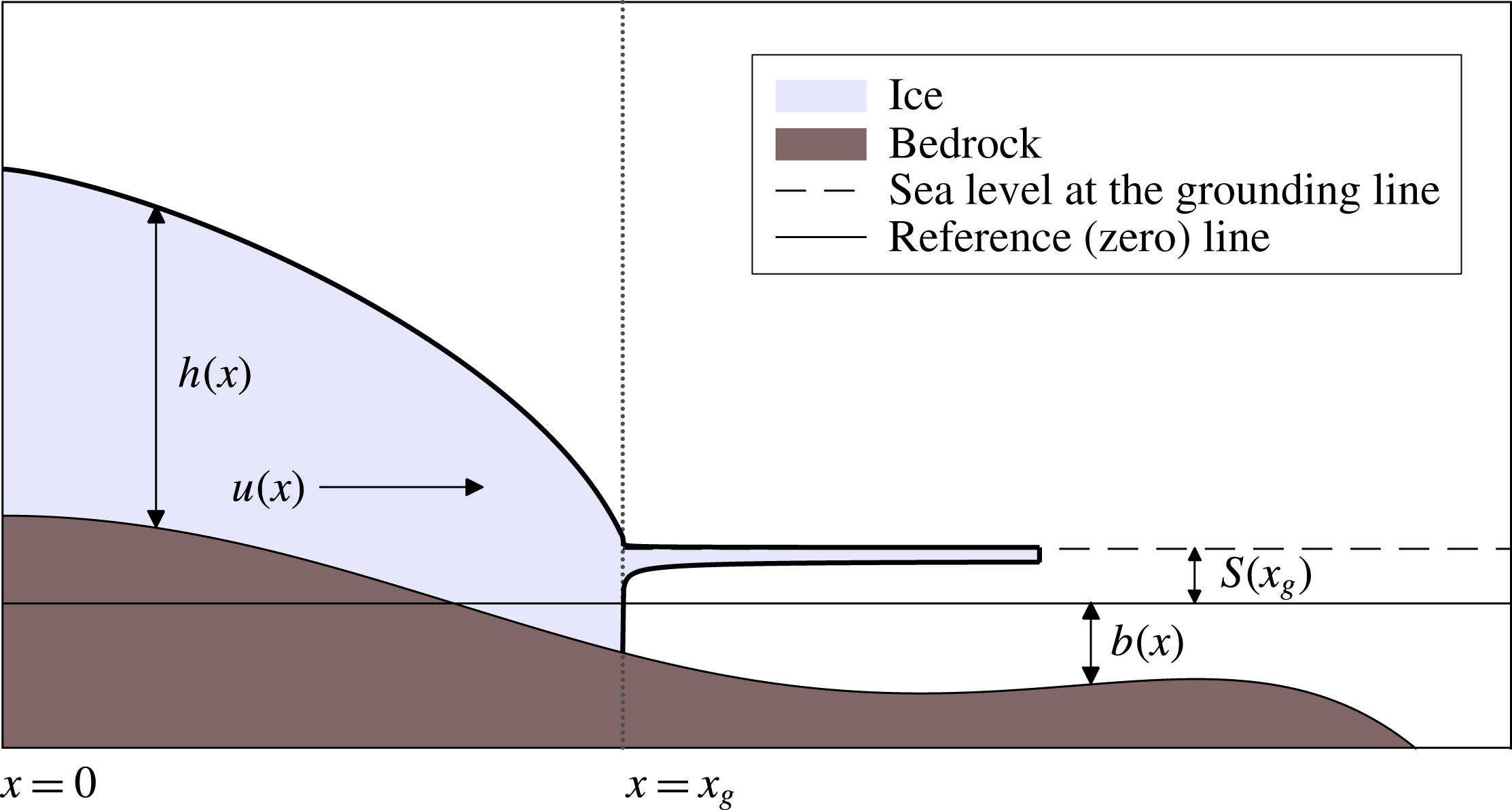
Consider in figure 1 a two-dimensional marine ice sheet situated on a bedrock topography in a Cartesian coordinate system, with a symmetry axis at
 $x=0$
. The grounding line is indicated by
 $x_{g}$
, the ice thickness by
 $h$
, the ice velocity by
 $u$
, the bedrock depth by
 $b$
and the sea level by
 $S$
.
A two-dimensional marine ice sheet. The ice thickness is given by
 $h(x)$
and the horizontal ice velocity by
 $u(x)$
. Up until the grounding line
 $x_{g}$
, the ice sheet rests on the bedrock
 $b(x)$
. At the grounding line the sea level is given by
 $S(x_{g})$
and the ice sheet extends into a floating ice shelf.
2.1 Model
The dynamics of the marine ice sheet is modelled using the shallow-shelf approximation (SSA), which is obtained by simplifying the full Stokes problem for gravity driven ice flow (Greve & Blatter Reference Greve and Blatter2009). The SSA, as implemented in Schoof (Reference Schoof2007a
), is a vertically integrated, two-dimensional model for a rapidly sliding ice sheet, and is used as a benchmark problem for the marine ice sheet intercomparison project (MISMIP) (Pattyn et al.
Reference Pattyn, Schoof, Perichon, Hindmarsh, Bueler, de Fleurian, Durand, Gagliardini, Gladstone and Goldberg2012), see also appendix C. Note that the SSA equations do not capture vertical gradients in horizontal velocity and hence neglect vertical shear. Thus,
 $u$
is a function of horizontal position only. Conservation of mass is expressed by
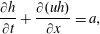 $$\begin{eqnarray}\displaystyle & \displaystyle \frac{\unicode[STIX]{x2202}h}{\unicode[STIX]{x2202}t}+\frac{\unicode[STIX]{x2202}(uh)}{\unicode[STIX]{x2202}x}=a, & \displaystyle\end{eqnarray}$$
where
 $a$
is the accumulation rate. Conservation of momentum is formulated as
 $$\begin{eqnarray}\displaystyle & \displaystyle \frac{\unicode[STIX]{x2202}}{\unicode[STIX]{x2202}x}\left[2A^{-1/n}h\left|\frac{\unicode[STIX]{x2202}u}{\unicode[STIX]{x2202}x}\right|^{(1/n)-1}\frac{\unicode[STIX]{x2202}u}{\unicode[STIX]{x2202}x}\right]-C|u|^{(m-1)}u-\unicode[STIX]{x1D70C}_{i}gh\frac{\unicode[STIX]{x2202}(h-b)}{\unicode[STIX]{x2202}x}=0, & \displaystyle\end{eqnarray}$$
where
 $A$
and
 $n$
are coefficients of Glen’s flow law, a constitutive relation describing the rheology of ice (Greve & Blatter (Reference Greve and Blatter2009), Van der Veen (Reference Van der Veen2013), typically
 $n=3$
). The ice density is given by
 $\unicode[STIX]{x1D70C}_{i}$
,
 $g$
is the gravitational acceleration and the bedrock depth and
 $b$
is taken positive in the downward direction. The consecutive terms in the momentum balance (2.2) represent longitudinal stress, basal shear stress and the driving stress respectively, where
 $C$
and
 $m$
determine the sliding of the ice. Note that the parameters
 $A,n$
and
 $C,m$
have an opposite physical significance: an increase in stress may be induced by an increase in
 $C$
,
 $m$
, and/or a decrease in
 $A$
,
 $n$
.
The left boundary of the domain (
 $x=0$
) is assumed to be located at an ice divide, a location in the ice with zero horizontal velocity. Hence, at the ice divide,
 $u=0$
and symmetry in thickness and bedrock depth requires a zero surface slope
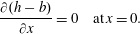 $$\begin{eqnarray}\displaystyle & \displaystyle \frac{\unicode[STIX]{x2202}(h-b)}{\unicode[STIX]{x2202}x}=0\quad \text{at}\,x=0. & \displaystyle\end{eqnarray}$$
There are two boundary conditions at the grounding line
 $x=x_{g}$
. One condition results from ice-shelf equations, with the same assumptions as used in deriving (2.1) and (2.2) (Weertman Reference Weertman1957). From a horizontal integration of shelf flow (Schoof Reference Schoof2007a
) it follows that
 $$\begin{eqnarray}\displaystyle & \displaystyle 2A^{-1/n}\left|\frac{\unicode[STIX]{x2202}u}{\unicode[STIX]{x2202}x}\right|^{(1/n)-1}\frac{\unicode[STIX]{x2202}u}{\unicode[STIX]{x2202}x}=\frac{1}{2}\left(1-{\displaystyle \frac{\unicode[STIX]{x1D70C}_{i}}{\unicode[STIX]{x1D70C}_{w}}}\right)\unicode[STIX]{x1D70C}_{i}gh\quad \text{at}\,x=x_{g}. & \displaystyle\end{eqnarray}$$
The other boundary condition is the flotation requirement:
 $$\begin{eqnarray}\displaystyle & \displaystyle \unicode[STIX]{x1D70C}_{i}h=\unicode[STIX]{x1D70C}_{w}\left(b+S\right)\quad \text{at}\,x=x_{g}, & \displaystyle\end{eqnarray}$$
where
 $S(x_{g})$
is the sea level at the grounding line position.
When an ice sheet melts, the additional water will raise the sea level (eustatic effect). However, the gravitational pull of the reduced ice mass on the water will also decrease, and hence sea level lowers. To determine the sea level
 $S$
due to the loading of the ice and the bedrock, we formally need to solve the sea level equation for this configuration. However, an easier representation was formulated in Gomez et al. (Reference Gomez, Mitrovica, Huybers and Clark2010), who show that sea level
 $S$
can be expressed as a single function of the grounding line position
 $x_{g}$
. In this case, the equation for the mean sea level (constant in
 $x$
) reduces to
 $$\begin{eqnarray}\displaystyle & \displaystyle \frac{\text{d}S}{\text{d}x_{g}}=f(x_{g}), & \displaystyle\end{eqnarray}$$
where
 $f$
is a function of
 $x_{g}$
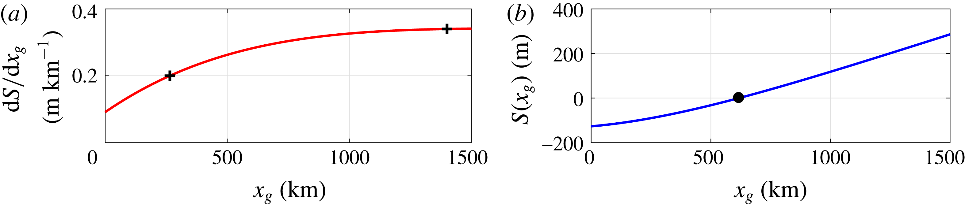
that can be determined from figure 2 in Gomez et al. (Reference Gomez, Mitrovica, Huybers and Clark2010).
(a) Fit of
 $\text{d}S/\text{d}x_{g}$
in Gomez et al. (Reference Gomez, Mitrovica, Huybers and Clark2010). Points corresponding to
 $0.20~\text{m}~\text{km}^{-1}$
at
 $x=265~\text{km}$
and
 $0.34~\text{m}~\text{km}^{-1}$
at
 $x=1400~\text{km}$
are marked with crosses. (b) Sea level as a function of
 $x_{g}$
. For the reference ice sheet we take
 $S(x_{g}=L_{i})=0$
, as is marked with a dot in the graph.
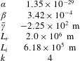
Here we will use a function of the form
 $$\begin{eqnarray}\displaystyle f(x_{g})=-\unicode[STIX]{x1D6FC}(x_{g}-L_{r})^{k}+\unicode[STIX]{x1D6FD}, & & \displaystyle\end{eqnarray}$$
where we choose
 $\unicode[STIX]{x1D6FC}$
,
 $\unicode[STIX]{x1D6FD}$
,
 $L_{r}$
and
 $k$
to fit the results in Gomez et al. (Reference Gomez, Mitrovica, Huybers and Clark2010), see figure 2(a). The coefficients
 $\unicode[STIX]{x1D6FC}$
and
 $\unicode[STIX]{x1D6FD}$
are fixed to match the correct range in sea level changes. The index
 $k$
and constant
 $L_{r}$
are chosen to mimic the nonlinearity of the curve, see table 1 for their values. Hence, the sea level
 $S(x_{g})$
is given by
 $$\begin{eqnarray}\displaystyle & \displaystyle S(x_{g})=-\frac{\unicode[STIX]{x1D6FC}}{k+1}(x_{g}-L_{r})^{k+1}+\unicode[STIX]{x1D6FD}x_{g}+\unicode[STIX]{x1D6FE}, & \displaystyle\end{eqnarray}$$
where
 $\unicode[STIX]{x1D6FE}$
is chosen such that the sea level for the reference solution is zero (see figure 2
b and § 3).
Coefficients for our fit of the gravitational sea level effect (GSLE) in Gomez et al. (Reference Gomez, Mitrovica, Huybers and Clark2010). The initial grounding line position
 $L_{i}$
and deterministic sea level correction
 $\bar{\unicode[STIX]{x1D6FE}}$
are determined after a starting solution with fixed sea level is obtained, see § 3.
We will assume noise in both the accumulation rate
 $a$
and the sea level according to
 $$\begin{eqnarray}\displaystyle a=\bar{a}+\unicode[STIX]{x1D702}_{ac}\unicode[STIX]{x1D701}(t), & & \displaystyle\end{eqnarray}$$
 $$\begin{eqnarray}\displaystyle \unicode[STIX]{x1D6FE}=\bar{\unicode[STIX]{x1D6FE}}+\unicode[STIX]{x1D702}_{sl}\unicode[STIX]{x1D701}(t), & & \displaystyle\end{eqnarray}$$
where the bar indicates the mean quantities,
 $\unicode[STIX]{x1D702}_{ac}$
and
 $\unicode[STIX]{x1D702}_{sl}$
the standard deviation of the accumulation and sea level noise, respectively and
 $\unicode[STIX]{x1D701}(t)$
is a Gaussian white noise process with unit variance, hence with
 $$\begin{eqnarray}\displaystyle E[\unicode[STIX]{x1D701}(t)]=0,\quad E[\unicode[STIX]{x1D701}(t)\unicode[STIX]{x1D701}(s)]=\unicode[STIX]{x1D6FF}(t-s), & & \displaystyle\end{eqnarray}$$
where
 $\unicode[STIX]{x1D6FF}$
is the Dirac delta function. Other parameters can be assumed to have a stochastic component as well. Uncertainty in the grounding line stress, caused for instance by buttressing, may be similarly parameterised (see appendix E).
Details on how the equations are non-dimensionalised and discretised on a staggered one-dimensional grid with spatial index
 $i=1,2,\ldots ,N$
are given in appendix A. The discretised problem can be formulated as a system of stochastic differential–algebraic equations (SDAE):
 $$\begin{eqnarray}\displaystyle \unicode[STIX]{x1D648}(\boldsymbol{x})\,\text{d}\boldsymbol{x}=F(\boldsymbol{x})\,\text{d}t+\unicode[STIX]{x1D63D}\,\text{d}\boldsymbol{W}, & & \displaystyle\end{eqnarray}$$
where
 $\boldsymbol{W}\in \mathbb{R}^{N_{w}}$
is a vector of
 $N_{w}$
independent standard Wiener processes and
 $\unicode[STIX]{x1D63D}\in \mathbb{R}^{(2N+1)\times N_{w}}$
controls the distribution of the noise in the system. Furthermore,
 $\boldsymbol{x}=(\boldsymbol{h},\boldsymbol{u},x_{g})^{\text{T}}\in \mathbb{R}^{2N+1}$
is the state vector, with
 $\boldsymbol{h},\boldsymbol{u}\in \mathbb{R}^{N}$
being the values of
 $h$
and
 $u$
at the grid points.
 $\unicode[STIX]{x1D648}\in \mathbb{R}^{(2N+1)\times (2N+1)}$
is a real-valued matrix with constant diagonal and non-constant off-diagonal coefficients, determined by the dependencies of the discretisation on time derivatives. Non-zero rows in
 $\unicode[STIX]{x1D648}$
correspond to differential equations, whereas the zero rows give a system of algebraic equations, hereafter referred to as ‘algebraic constraints’. Finally,
 $F:\mathbb{R}^{2N+1}\rightarrow \mathbb{R}^{2N+1}$
is a nonlinear operator arising from the spatial discretisation. Explicit expressions for the deterministic components are given by
 $$\begin{eqnarray}\displaystyle \unicode[STIX]{x1D648}=\left[\begin{array}{@{}ccc@{}}\unicode[STIX]{x1D644} & 0 & M_{str}(\boldsymbol{h},x_{g})\\ 0 & 0 & 0\\ 0 & 0 & 0\end{array}\right],\quad F=\left[\begin{array}{@{}c@{}}F_{mass}(\boldsymbol{h},\boldsymbol{u},x_{g})\\ F_{mom}(\boldsymbol{h},\boldsymbol{u},x_{g})\\ F_{flot}(\boldsymbol{h},x_{g})\end{array}\right], & & \displaystyle\end{eqnarray}$$
where
 $\unicode[STIX]{x1D644}\in \mathbb{R}^{N\times N}$
is the identity matrix and
 $M_{str}(\boldsymbol{h},x_{g})\in \mathbb{R}^{N}$
is the discretisation of the left-hand side of (A 16)–(A 21).
 $F_{mass}(\boldsymbol{h},\boldsymbol{u},x_{g})\in \mathbb{R}^{N}$
is given by the right-hand side of (A 16)–(A 21). Similarly,
 $F_{mom}(\boldsymbol{h},\boldsymbol{u},x_{g})\in \mathbb{R}^{N}$
and
 $F_{flot}(\boldsymbol{h},\boldsymbol{u},x_{g})\in \mathbb{R}$
are given by the right-hand sides of the discretised momentum equation and flotation criterion (A 22)–(A 23). Explicit expressions for the noise distributions
 $\unicode[STIX]{x1D63D}$
are given in § 4.
2.2 Pseudo-arclength continuation
The deterministic part of (2.12) gives a problem of the form
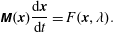 $$\begin{eqnarray}\displaystyle & \displaystyle \unicode[STIX]{x1D648}(\boldsymbol{x})\frac{\text{d}\boldsymbol{x}}{\text{d}t}=F(\boldsymbol{x},\unicode[STIX]{x1D706}). & \displaystyle\end{eqnarray}$$
We explicitly introduce the parameter dependence
 $\unicode[STIX]{x1D706}$
since we are interested in solution branches
 $(\boldsymbol{x},\unicode[STIX]{x1D706})$
satisfying
 $F(\boldsymbol{x},\unicode[STIX]{x1D706})=0$
. For example, the main parameter of interest is the coefficient
 $A$
in Glen’s flow law, which is affected by the external (global mean) temperature. We use a continuation method to compute branches of stable and unstable steady states
 $(\boldsymbol{x},\unicode[STIX]{x1D706})$
, obtain perturbations that describe (de)stabilising mechanisms and identify bifurcations. Here we will give a brief overview of the continuation procedure.
Various continuation techniques exist to trace a stationary solution branch while varying a parameter. An efficient approach is to parameterise a solution branch with a pseudo-arclength parameter
 $s$
(Keller Reference Keller1977), i.e.
 $(\boldsymbol{x}(s),\unicode[STIX]{x1D706}(s))$
, and impose an approximate normalisation condition on the tangent to close the system of equations:
 $\dot{\boldsymbol{x}}^{\text{T}}(\boldsymbol{x}-\boldsymbol{x}_{0})+\dot{\unicode[STIX]{x1D706}}(\unicode[STIX]{x1D706}-\unicode[STIX]{x1D706}_{0})-\unicode[STIX]{x0394}s=0$
, where
 $(\boldsymbol{x}_{0},\unicode[STIX]{x1D706}_{0})$
is an initial known stationary solution,
 $(\dot{\boldsymbol{x}},\dot{\unicode[STIX]{x1D706}})$
the tangent with respect to the arclength parameter at
 $(\boldsymbol{x}_{0},\unicode[STIX]{x1D706}_{0})$
and
 $\unicode[STIX]{x0394}s$
a specified step size.
To find a new point on the solution branch a predictor–corrector method is used. A suitable tangent predictor is given by
 $$\begin{eqnarray}\displaystyle & \displaystyle \boldsymbol{x}^{1}=\boldsymbol{x}_{0}+\unicode[STIX]{x0394}s~\dot{\boldsymbol{x}}, & \displaystyle\end{eqnarray}$$
 $$\begin{eqnarray}\displaystyle & \displaystyle \unicode[STIX]{x1D706}^{1}=\unicode[STIX]{x1D706}_{0}+\unicode[STIX]{x0394}s~\dot{\unicode[STIX]{x1D706}}. & \displaystyle\end{eqnarray}$$
Note that the predicted solution is denoted by
 $(\boldsymbol{x}^{1},\unicode[STIX]{x1D706}^{1})$
, whereas an actual new point on the branch will be denoted by
 $(\boldsymbol{x}_{1},\unicode[STIX]{x1D706}_{1})$
. The correction onto the solution branch is made through the solution of the nonlinear system given by
 $$\begin{eqnarray}\displaystyle & \displaystyle F(\boldsymbol{x},\unicode[STIX]{x1D706})=0, & \displaystyle\end{eqnarray}$$
 $$\begin{eqnarray}\displaystyle & \displaystyle \dot{\boldsymbol{x}}^{\text{T}}(\boldsymbol{x}-\boldsymbol{x}_{0})+\dot{\unicode[STIX]{x1D706}}(\unicode[STIX]{x1D706}-\unicode[STIX]{x1D706}_{0})-\unicode[STIX]{x0394}s=0. & \displaystyle\end{eqnarray}$$
A Newton–Raphson root finding procedure, initialised with the prediction
 $(\boldsymbol{x}^{1},\unicode[STIX]{x1D706}^{1})$
, gives the following iteration:
 $$\begin{eqnarray}\displaystyle \left[\begin{array}{@{}cc@{}}\unicode[STIX]{x1D645} & F_{\unicode[STIX]{x1D706}}\\ \dot{\boldsymbol{x}}^{\text{T}} & \dot{\unicode[STIX]{x1D706}}\end{array}\right]\left[\begin{array}{@{}c@{}}\unicode[STIX]{x0394}\boldsymbol{x}\\ \unicode[STIX]{x0394}\unicode[STIX]{x1D706}\end{array}\right]=\left[\begin{array}{@{}c@{}}-F(\boldsymbol{x}^{k},\unicode[STIX]{x1D706})\\ \unicode[STIX]{x0394}s-\dot{\boldsymbol{x}}^{\text{T}}(\boldsymbol{x}^{k}-\boldsymbol{x}_{0})-\dot{\unicode[STIX]{x1D706}}(\unicode[STIX]{x1D706}^{k}-\unicode[STIX]{x1D706}_{0})\end{array}\right], & & \displaystyle\end{eqnarray}$$
where
 $\unicode[STIX]{x0394}\boldsymbol{x}:=\boldsymbol{x}^{k+1}-\boldsymbol{x}^{k}$
,
 $\unicode[STIX]{x0394}\unicode[STIX]{x1D706}:=\unicode[STIX]{x1D706}^{k+1}-\unicode[STIX]{x1D706}^{k}$
and
 $\unicode[STIX]{x1D645}$
is the Jacobian matrix of
 $F$
. If this iteration converges a new stationary solution
 $(\boldsymbol{x}_{1},\unicode[STIX]{x1D706}_{1})$
has been found. At a fold bifurcation the Jacobian matrix
 $\unicode[STIX]{x1D645}$
will have a zero eigenvalue, yet the system in (2.19) remains non-singular and the continuation is able to trace the solution branch into its unstable domain.
When a stationary solution
 $\bar{\boldsymbol{x}}$
, satisfying
 $F(\bar{\boldsymbol{x}},\unicode[STIX]{x1D706})=0$
has been found, its linear stability can be investigated with a perturbation
 $\bar{\boldsymbol{x}}+\tilde{\boldsymbol{x}}$
and a linearisation around the stationary solution. The evolution of
 $\tilde{\boldsymbol{x}}$
follows from
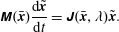 $$\begin{eqnarray}\displaystyle & \displaystyle \unicode[STIX]{x1D648}(\bar{\boldsymbol{x}})\frac{\text{d}\tilde{\boldsymbol{x}}}{\text{d}t}=\unicode[STIX]{x1D645}(\bar{\boldsymbol{x}},\unicode[STIX]{x1D706})\tilde{\boldsymbol{x}}. & \displaystyle\end{eqnarray}$$
See appendix B for details. Solutions of (2.20) are of the form
 $\tilde{\boldsymbol{x}}=\hat{\boldsymbol{x}}~\text{exp}\left(\unicode[STIX]{x1D70E}t\right)$
. Substitution gives a sparse generalised eigenvalue problem that needs to be solved numerically:
 $$\begin{eqnarray}\displaystyle & \displaystyle \unicode[STIX]{x1D70E}\unicode[STIX]{x1D648}(\bar{\boldsymbol{x}})\hat{\boldsymbol{x}}=\unicode[STIX]{x1D645}(\bar{\boldsymbol{x}},\unicode[STIX]{x1D706})\hat{\boldsymbol{x}}. & \displaystyle\end{eqnarray}$$
The stability of a stationary solution depends on the sign of the real part of the eigenvalues, i.e. if we find an eigenvalue with a positive real part the steady solution is unstable.
2.3 Variability under small noise approximation
With the continuation method described above we find linearly stable and unstable steady states
 $\bar{\boldsymbol{x}}$
of the deterministic part in (2.12). Linearising the stochastic equations around a deterministic equilibrium gives
 $$\begin{eqnarray}\displaystyle \unicode[STIX]{x1D648}~\text{d}\tilde{\boldsymbol{x}}=\unicode[STIX]{x1D645}~\tilde{\boldsymbol{x}}~\text{d}t+\unicode[STIX]{x1D63D}~\text{d}\boldsymbol{W}, & & \displaystyle\end{eqnarray}$$
for the perturbation
 $\tilde{\boldsymbol{x}}=\boldsymbol{x}-\bar{\boldsymbol{x}}$
with zero mean
 $\langle \tilde{\boldsymbol{x}}\rangle =0$
.
Now
 $\unicode[STIX]{x1D648}$
is obviously not invertible, but in §§ 4.1 and 4.2 below we will show that for both noise in the accumulation and in the sea level, the problem (2.22) can be written as a multivariate Ornstein–Uhlenbeck (OU) process:
 $$\begin{eqnarray}\displaystyle & \displaystyle \text{d}\boldsymbol{y}={\mathcal{M}}^{-1}{\mathcal{J}}\boldsymbol{y}~\text{d}t+{\mathcal{M}}^{-1}{\mathcal{B}}~\text{d}\boldsymbol{{\mathcal{W}}}, & \displaystyle\end{eqnarray}$$
with modified matrices
 ${\mathcal{M}},{\mathcal{J}},{\mathcal{B}}$
and
 ${\mathcal{W}}$
and a modified state vector
 $\boldsymbol{y}$
, with steady state
 $\bar{\boldsymbol{y}}$
(cf. (4.4) and (4.11)). A stationary covariance matrix
 ${\mathcal{C}}=E[\boldsymbol{y}\boldsymbol{y}^{\text{T}}]$
is obtained from the generalised Lyapunov equation (Gardiner Reference Gardiner2009; Kuehn Reference Kuehn2012; Baars et al.
Reference Baars, Viebahn, Mulder, Kuehn, Wubs and Dijkstra2017)
 $$\begin{eqnarray}\displaystyle & \displaystyle {\mathcal{J}}{\mathcal{C}}{\mathcal{M}}^{\text{T}}+{\mathcal{M}}{\mathcal{C}}{\mathcal{J}}^{\text{T}}+{\mathcal{B}}{\mathcal{B}}^{\text{T}}=0. & \displaystyle\end{eqnarray}$$
Once
 ${\mathcal{C}}$
is computed, the covariance matrix
 $\unicode[STIX]{x1D63E}=E[\boldsymbol{x}\boldsymbol{x}^{\text{T}}]$
can be obtained (Baars et al.
Reference Baars, Viebahn, Mulder, Kuehn, Wubs and Dijkstra2017), which allows the computation of the stationary probability density function, indicated by
 $p(\tilde{\boldsymbol{x}};\bar{\boldsymbol{x}})$
, as (Gardiner Reference Gardiner2009)
 $$\begin{eqnarray}\displaystyle & \displaystyle p(\tilde{\boldsymbol{x}};\bar{\boldsymbol{x}})={\displaystyle \frac{1}{(2\unicode[STIX]{x03C0})^{d/2}}}\mid \unicode[STIX]{x1D63E}\mid ^{-1/2}\text{e}^{-1/2(\tilde{\boldsymbol{x}}-\bar{\boldsymbol{x}})^{\text{T}}\unicode[STIX]{x1D63E}^{-1}(\tilde{\boldsymbol{x}}-\bar{\boldsymbol{x}})}, & \displaystyle\end{eqnarray}$$
where
 $d=2N+1$
is the dimension of the state vector
 $\boldsymbol{x}$
.
One limitation of this approach is that the obtained probability density function is only valid on a subexponential time scale, i.e. before large deviations occur. Secondly, only the local behaviour near the steady state and Gaussian stochastic behaviour of the perturbation state vector are obtained.
3 Results: deterministic model
In this section, we will focus on the steady states of the deterministic model and the existence of multiple equilibrium regimes (§ 3.1). Furthermore, using the linear stability analyses, a novel, more detailed view on the marine ice sheet bifurcation behaviour is presented (§ 3.2). In § 3.3 we will study the impact of the gravitational sea level effect on the stability of the marine ice sheet.
3.1 Bifurcation diagram
We consider the case of constant accumulation
 $a=\bar{a}$
, flat sea level, i.e.
 $S(x_{g})=0$
and a fixed shape of the bedrock
 $b(x)$
given by (Schoof Reference Schoof2007a
):
 $$\begin{eqnarray}\displaystyle & \displaystyle b(x)=-\!\left(729-2184.8\left({\displaystyle \frac{x}{L_{B}}}\right)^{2}+1031.72\left({\displaystyle \frac{x}{L_{B}}}\right)^{4}-151.72\left({\displaystyle \frac{x}{L_{B}}}\right)^{6}\right), & \displaystyle\end{eqnarray}$$
with
 $L_{B}=750\times 10^{3}~\text{m}$
. To obtain a starting solution for the continuation it is possible to use the boundary layer theory developed in Schoof (Reference Schoof2007b
). However, we found that an ice sheet surface profile of the form
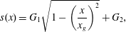 $$\begin{eqnarray}\displaystyle & \displaystyle s(x)=G_{1}\sqrt{1-\left({\displaystyle \frac{x}{x_{g}}}\right)^{2}}+G_{2}, & \displaystyle\end{eqnarray}$$
with
 $x\in [0,x_{g}]$
, is sufficient to give an initial state that will rapidly converge to a stationary (starting) solution using the Newton–Raphson method. The initial ice sheet thickness is then given by
 $h(x)=s(x)+b(x)$
and the initial velocity follows from assuming steady conditions and integrating the continuity equation:
 $$\begin{eqnarray}\displaystyle & \displaystyle u(x)=\frac{\bar{a}\,x}{h(x)}. & \displaystyle\end{eqnarray}$$
A typical height is chosen with
 $G_{1}=3\times 10^{3}$
m and a correction
 $G_{2}$
(in m) is used such that the flotation criterion (2.5) is satisfied:
 $G_{2}=(\unicode[STIX]{x1D70C}_{w}/\unicode[STIX]{x1D70C}_{i}-1)b(x_{g})$
, where we use that the sea level
 $S(x_{g})=0$
at the starting solution. Note that the profile (3.2) contains a steep gradient at the grounding line, which is essential for a converging Newton–Raphson iteration to a starting solution. The continuation in
 $A$
is initialised with a solution at
 $A_{0}=4.6416\times 10^{-24}$
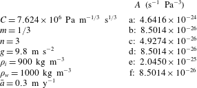
. All other model parameters are given in table 2.
One-parameter bifurcation diagram (a) and solutions (b) with the parameter
 $A$
. The bedrock contains an upward slope which admits multiple steady states for a constant parameter (points b, d and f in panel (a)). Eigenvalue analysis shows two saddle-node bifurcations,
 $L_{1}$
and
 $L_{2}$
: a single eigenvalue crosses the imaginary axis to the positive right half plane at point c and returns to the left half plane at point e. The number of grid-points is
 $N=1600$
; the other parameters are given in table 2.
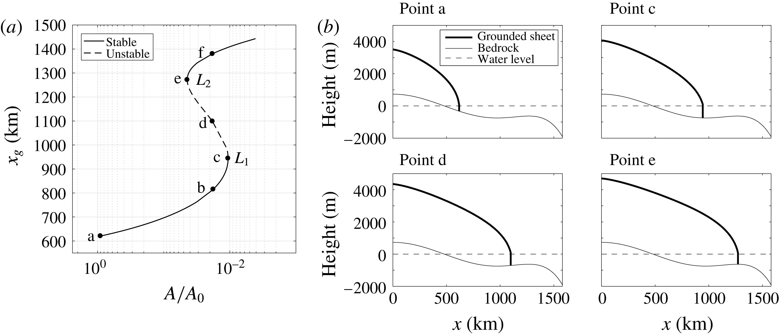
From the steady starting solution at
 $A_{0}$
, a pseudo-arclength continuation traces the solution branch in the direction of decreasing
 $A$
, see figure 3. A decrease in the parameter
 $A$
in the SSA model corresponds to a decrease in temperature and an increase in ice growth. The bifurcation diagram presented reveals the multiple equilibria regime associated with hysteretic behaviour (Schoof Reference Schoof2007a
). For an interval of values of the parameter
 $A$
, three equilibria are distinguished for the case
 $A=8.5014\times 10^{-26}$
, marked with labels b, d and f in figure 3. At point c, an eigenvalue of (2.21) is found to cross the imaginary axis to the right half-plane, coinciding with the annihilation of a stable and an unstable branch in the direction of decreasing
 $A$
. Hence a saddle-node bifurcation is identified (
 $L_{1}$
). At point e, the same eigenvalue returns to the left half-plane through a second saddle-node bifurcation (
 $L_{2}$
). The values of the parameter
 $A$
at the labelled points, including the bifurcations, are shown in table 2.
Parameter values for the experiment in figure 3, similar to the values chosen in Schoof (Reference Schoof2007a ) and Pattyn et al. (Reference Pattyn, Schoof, Perichon, Hindmarsh, Bueler, de Fleurian, Durand, Gagliardini, Gladstone and Goldberg2012).
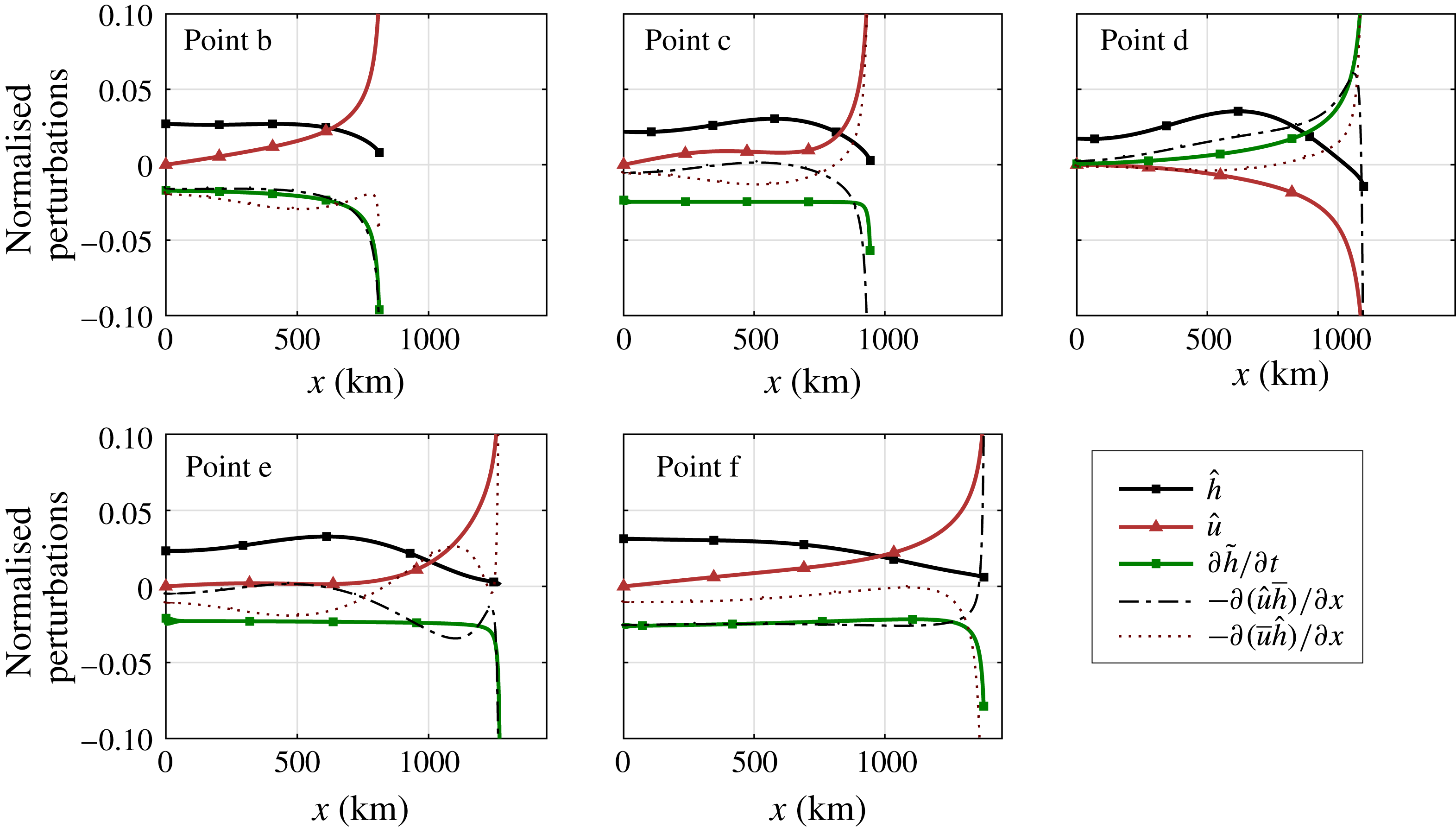
Normalised components of the eigenmode that becomes unstable. The corresponding steady states are located at points b–f, described in figure 3 and table 2. We distinguish between a perturbation pattern related to sheet thickness
 ${\hat{h}}$
and a pattern related to ice velocity
 $\hat{u}$
. The signs of the eigenvectors are taken such that the perturbation in the grounding line is positive. From the eigenvectors and the equilibrium solution we compute a normalised spatial pattern of the evolution
 $\unicode[STIX]{x2202}\tilde{h}/\unicode[STIX]{x2202}t$
, together with normalised components
 $-\unicode[STIX]{x2202}(\hat{u} \bar{h})/\unicode[STIX]{x2202}x$
and
 $-\unicode[STIX]{x2202}(\bar{u}{\hat{h}})/\unicode[STIX]{x2202}x$
.
3.2 Instability mechanism
The advantage of the approach chosen here is that the spatial patterns of perturbations destabilising the marine ice sheet can be determined from the eigenvectors in (2.21). For the unstable equilibrium (point d) in figure 3, it is of interest to examine the eigenmode with a positive growth factor, showing in detail the characteristics of the instability. The eigenvector is made available using (2.21) and is depicted for the steady states (points b–f) in figure 4. The perturbations in thickness and velocity are taken corresponding to a positive grounding line perturbation. Note that a perturbation of the solution vector has the form
 $\hat{\boldsymbol{x}}\text{e}^{\unicode[STIX]{x1D70E}t}=[\hat{\boldsymbol{h}},\hat{\boldsymbol{u}},\hat{x}_{g}]^{\text{T}}\text{e}^{\unicode[STIX]{x1D70E}t}$
, with
 $\hat{x}_{g}$
the scalar grounding line perturbation. An eigenvector with corresponding eigenvalue
 $\unicode[STIX]{x1D70E}>0$
and
 $\hat{x}_{g}<0$
gives the destabilising pattern for unstable ice sheet retreat. By adjusting the sign of the eigenvector, such that
 $\hat{x}_{g}>0$
, we restrict our exposition to destabilising patterns for unstable ice sheet growth.
At the grounding line
 $x_{g}$
, the perturbation of the unstable steady state (point d) shows a slight decrease in ice thickness, while at (points b, c, e and f) a slight increase is observed. In the interior of the ice sheet a relatively large increase in ice thickness is visible for the unstable equilibrium (point d), indicating interior ice growth due to an imbalance between global accumulation and ice flux at the grounding line. That is, the reduced grounding line ice discharge is unable to accommodate the increased accumulation. The resulting interior thickness anomaly is central to the unstable growth/retreat mechanism, as we will see next.
The velocity perturbation at the grounding line shows an increase for stable states and a clear decrease for the unstable state (point d). Together with the negative perturbation in thickness this implies that, at (point d), there must be a decrease in flux
 $uh$
across the grounding line for a positive perturbation
 $\hat{x}_{g}>0$
. An increase in grounding line position implies a rise in global accumulation, hence the reduction in grounding line flux implies a net ice growth, confirming the marine ice sheet instability hypothesis. Note that a similar result holds if we take the perturbation in
 $x_{g}$
negative, giving a net ice loss and a retreat from equilibrium.
The continuation approach allows an efficient computation of flux perturbations using (2.21). From a linear stability analysis of (2.1) with perturbation
 $\tilde{h}=c{\hat{h}},~\tilde{u} =c\hat{u}$
around an equilibrium
 $\bar{h},\bar{u}$
we obtain an evolution equation for the thickness perturbation
 $\tilde{h}$
:
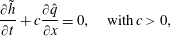 $$\begin{eqnarray}\displaystyle & \displaystyle \frac{\unicode[STIX]{x2202}\tilde{h}}{\unicode[STIX]{x2202}t}+c\frac{\unicode[STIX]{x2202}\hat{q}}{\unicode[STIX]{x2202}x}=0,\quad \text{with}\,c>0, & \displaystyle\end{eqnarray}$$
 $$\begin{eqnarray}\displaystyle & \displaystyle \hat{q}(x)=\hat{u} \bar{h}+\bar{u}{\hat{h}}, & \displaystyle\end{eqnarray}$$
where we neglect higher-order terms. At the unstable steady state (point d) in figure 4, the thickness perturbation (green squares) shows positive growth, whereas the other points show a dampening. These patterns are determined by spatial derivatives of the perturbed advection of the steady thickness
 $\hat{u} \bar{h}$
(black dash-dotted line) and the advected thickness perturbation
 $\bar{u}{\hat{h}}$
(red dotted line). The latter clearly dominates the instability in (point d). Note that at the bifurcation points c and e the components of the perturbation flux have a compensating effect.
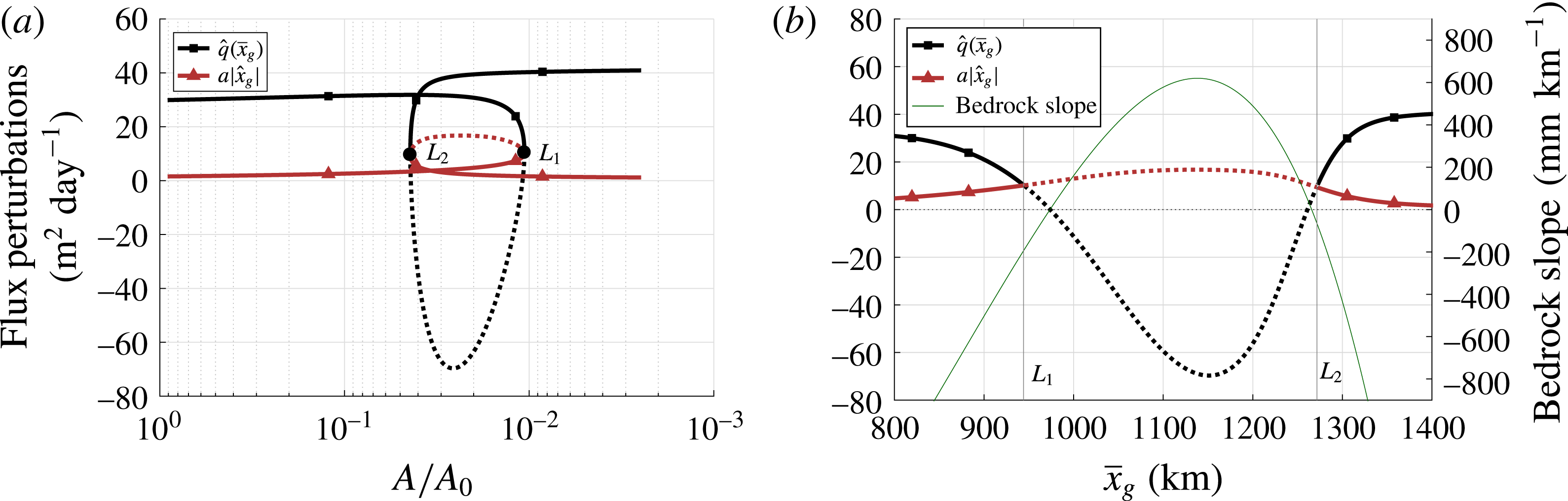
Perturbations in grounding line and accumulation flux against the parameter
 $A$
(a) and as a function of
 $x_{g}$
(b), together with the bedrock slope. The first and second saddle-node bifurcations are marked
 $L_{1}$
and
 $L_{2}$
. Dashed lines correspond to growing perturbations of unstable steady states. The perturbations
 $\hat{q}(\bar{x}_{g})$
and
 $a|\hat{x}_{g}|$
correspond to a positive grounding line perturbation
 $\hat{x}_{g}>0$
. At
 $L_{1}$
and
 $L_{2}$
, the grounding line bedrock slope is
 $-195~\text{mm}~\text{km}^{-1}$
and
 $-65~\text{mm}~\text{km}^{-1}$
respectively. The maximum slope in the unstable regime is
 $620~\text{mm}~\text{km}^{-1}$
. Note that grounding line flux perturbations depend on the steady grounding line position
 $\bar{x}_{g}$
, whereas accumulation flux perturbations depend on the grounding line perturbation
 $\hat{x}_{g}$
.
To investigate how a perturbation changes from stable to unstable through the saddle-node bifurcation
 $L_{1}$
, we compute the accumulation and grounding line fluxes. The steady state
 $(\bar{h},\bar{u})$
gives a balance:
 $$\begin{eqnarray}\displaystyle & \displaystyle \bar{q}(x)=\bar{u}\bar{h}=ax. & \displaystyle\end{eqnarray}$$
In figure 5 we show perturbations of the balance (3.6) at the grounding line. A perturbation in accumulation flux is given by
 $a|\hat{x}_{g}|$
, a grounding line flux perturbation by
 $\hat{q}(\bar{x}_{g})$
in (3.4). The perturbations are plotted against
 $A/A_{0}$
(figure 5
a) and
 $\bar{x}_{g}$
(figure 5
b), together with the bifurcation points and the bedrock slope. At the first saddle-node bifurcation
 $L_{1}$
, the flux
 $\hat{q}(x_{g})$
becomes smaller than the accumulation
 $a|\hat{x}_{g}|$
. Beyond this point, a change in accumulation due to
 $\hat{x}_{g}$
is not balanced by the grounding line flux and, hence, the perturbation
 $\tilde{\boldsymbol{x}}$
changes from damped to growing. At
 $L_{2}$
,
 $\hat{q}(x_{g})$
becomes greater than
 $a|\hat{x}_{g}|$
and the mode is damped again.
In figure 5(b) we also plot the bedrock slope, taken positive when the bed elevation increases with
 $x_{g}$
, that is
 $$\begin{eqnarray}\displaystyle & \displaystyle r_{bed}=-b^{\prime }(x_{g}), & \displaystyle\end{eqnarray}$$
with
 $b(x)$
as in (3.1). Note that the sign switch in
 $\hat{q}(x_{g})$
coincides with the sign switch in the bedrock slope. The grounding line flux will increase for a positive
 $\hat{x}_{g}$
between the bifurcation
 $L_{1}$
and the point of zero bedrock slope, but, since the change is less than the change in accumulation, the ice sheet will grow. Thus, figure 5 confirms that an eigenvalue of the ‘full model’ in Schoof (Reference Schoof2007a
) becomes positive when
 $$\begin{eqnarray}\displaystyle & \displaystyle a|\hat{x}_{g}|-\hat{q}(x_{g})>0. & \displaystyle\end{eqnarray}$$
Using a continuation of steady states with the original SSA equations, we find that the flux perturbations and their relative magnitude fully describe the instability mechanism, confirming the analysis in Schoof (Reference Schoof2012), but without the need for asymptotic expansions. In addition, the eigenvectors reveal destabilising interior patterns with, most interestingly, interior thickness anomalies and their advection. These turn out to play a major role in the growth and retreat of the ice sheet.
3.3 Gravitational sea level effect
Next, instead of a fixed
 $S(x)=0$
, we use the gravitational sea level effect (GSLE) formulation given by (2.8). With the added sea level we repeat the continuation in the parameter
 $A$
(§ 3.1). The new bifurcation diagram is shown in figure 6(a) (red triangles). The width of the multiple equilibria regime has decreased significantly and the bifurcations have shifted in the direction of decreasing
 $A$
. The same grounding line advance now requires a greater decrease in
 $A$
compared to the fixed sea level case. The parameter difference between the saddle-node bifurcations with fixed sea level is
 $|A_{L_{2}}-A_{L_{1}}|/A_{0}=3.34\times 10^{-2}$
; for the variable sea level case we find
 $|A_{S_{2}}-A_{S_{1}}|/A_{0}=3.18\times 10^{-3}$
. Here we denote the parameter values at the bifurcations
 $L_{1},L_{2},S_{1}$
and
 $S_{2}$
with
 $A_{L_{1}},A_{L_{2}},A_{S_{1}}$
and
 $A_{S_{2}}$
respectively. The unstable regime has a horizontal extent of approximately 326 km in the fixed sea level case; for the variable sea level case we find 248 km.
(a) Bifurcation diagrams in the parameter
 $A$
. Fixed sea level bifurcation diagram (black) and bifurcation diagram with variable sea level (red). (b) Accumulation and grounding line flux perturbations as a function of
 $x_{g}$
for variable sea level, together with the bedrock slope and the resulting effective topographical slope. The first and second saddle-node bifurcations are marked
 $L_{1}$
(
 $S_{1}$
) and
 $L_{2}$
(
 $S_{2}$
) for fixed (variable) sea level. Dashed lines correspond to (perturbations of) unstable steady states.
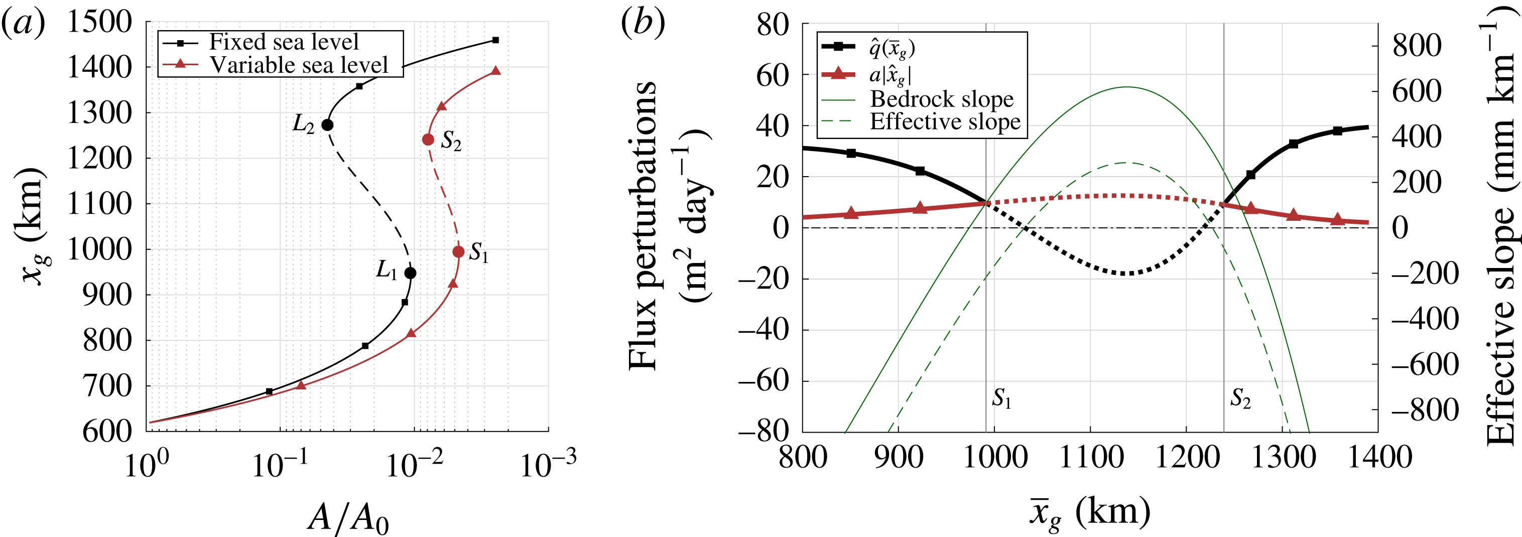
Changes in the instability mechanism due to the presence of a varying sea level are investigated using the eigenvectors from the linear stability analysis (2.21). In figure 6(b), the perturbation in flux intersects the perturbation in accumulation at
 $S_{1}$
and the ice sheet state becomes unstable. At the second saddle-node bifurcation
 $S_{2}$
the reverse occurs. Both sign switches in bedrock slope are now located in the stable regime. This confirms that, for our choice of sea level response, a reverse bed slope is reduced from a sufficient to a necessary condition for the instability mechanism.
In figure 6(b) we also plot the effective topographic slope, taken positive when the bed elevation increases with
 $x_{g}$
, that is
 $$\begin{eqnarray}\displaystyle & \displaystyle r_{eff}=-(b^{\prime }(x_{g})+S^{\prime }(x_{g})). & \displaystyle\end{eqnarray}$$
Similar to the fixed sea level case, there is a direct correspondence between the grounding line flux perturbation and the effective topography. Note also that the magnitudes of the fluxes in the unstable regime are strongly affected by the magnitude of the slope. Hence, the dampening effect of the added variable sea level acts through the response of the unstable flux perturbations to the significantly decreased effective slope, in agreement with the analysis in Gomez et al. (Reference Gomez, Mitrovica, Huybers and Clark2010). Whether the dampening extends to the stochastic case is explored in the next section.
4 Stochastic variability
In this section, we present the results for the stochastic model with a variable (GSLE) sea level. In §§ 4.1 and 4.2, we consider separate noise in the accumulation rate and sea level amplitude and in § 4.3 we study the variability due to both types of noise on a deterministically stable ice sheet. Finally, in § 4.4 we consider the transition probabilities between different ice sheet states in multiple equilibrium regimes.
4.1 Additive noise in the accumulation rate
The linearised system of SDAEs (cf. (2.22)) that arises when adding noise to the accumulation
 $a$
is given by
 $$\begin{eqnarray}\displaystyle \unicode[STIX]{x1D648}\,\text{d}\tilde{\boldsymbol{x}}=\unicode[STIX]{x1D645}\tilde{\boldsymbol{x}}~\text{d}t+\left[\begin{array}{@{}c@{}}B_{a}\\ 0\\ 0\\ \end{array}\right]\text{d}\boldsymbol{W},\quad \text{with}~\tilde{\boldsymbol{x}}=\left[\begin{array}{@{}c@{}}\tilde{\boldsymbol{h}}\\ \tilde{\boldsymbol{u}}\\ \tilde{x}_{g}\end{array}\right]\text{ and}~\unicode[STIX]{x1D648}=\left[\begin{array}{@{}ccc@{}}\unicode[STIX]{x1D644} & 0 & M_{str}\\ 0 & 0 & 0\\ 0 & 0 & 0\end{array}\right], & & \displaystyle\end{eqnarray}$$
where
 $\unicode[STIX]{x1D645}$
denotes the Jacobian matrix. As the accumulation is taken uniform over the sheet, the additive noise is integrated with respect to a one-dimensional Wiener process, that is,
 $N_{w}=1$
and
 $B_{a}\in \mathbb{R}^{N}$
with elements
 $(B_{a})_{i}=\unicode[STIX]{x1D702}_{ac}$
, where
 $\unicode[STIX]{x1D702}_{ac}$
(
 $\text{my}^{-1}$
) determines the noise amplitude and is taken at 10 % of the accumulation constant.
The matrix
 $\unicode[STIX]{x1D648}$
in the left-hand side of (4.1) is not invertible. In order to achieve a problem of the form (2.23), we need to bring
 $\unicode[STIX]{x1D648}$
in block-diagonal form and eliminate the system of algebraic equations. The transformation
 $\tilde{\boldsymbol{x}}=\unicode[STIX]{x1D64D}\boldsymbol{z}$
with
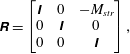 $$\begin{eqnarray}\displaystyle \unicode[STIX]{x1D64D}=\left[\begin{array}{@{}ccc@{}}\unicode[STIX]{x1D644} & 0 & -M_{str}\\ 0 & \unicode[STIX]{x1D644} & 0\\ 0 & 0 & \unicode[STIX]{x1D644}\end{array}\right], & & \displaystyle\end{eqnarray}$$
gives a system of SDAEs in a more convenient form:
 $$\begin{eqnarray}\displaystyle \left[\begin{array}{@{}cc@{}}\unicode[STIX]{x1D644} & 0\\ 0 & 0\end{array}\right]\left[\begin{array}{@{}c@{}}\text{d}\,\boldsymbol{z}_{1}\\ \text{d}\,\boldsymbol{z}_{2}\end{array}\right]=\left[\begin{array}{@{}cc@{}}\unicode[STIX]{x1D645}_{11} & \unicode[STIX]{x1D645}_{12}\\ \unicode[STIX]{x1D645}_{21} & \unicode[STIX]{x1D645}_{22}\end{array}\right]\unicode[STIX]{x1D64D}\left[\begin{array}{@{}c@{}}\boldsymbol{z}_{1}\\ \boldsymbol{ z}_{2}\end{array}\right]\text{d}t+\left[\begin{array}{@{}c@{}}B_{a}\\ 0\end{array}\right]\text{d}\boldsymbol{W}, & & \displaystyle\end{eqnarray}$$
where the second row combines the algebraic constraints and provides an expression for
 $\boldsymbol{z}_{2}$
in terms of
 $\boldsymbol{z}_{1}$
. Substituting this expression in the first row eliminates
 $\boldsymbol{z}_{2}$
from (4.3) (Baars et al.
Reference Baars, Viebahn, Mulder, Kuehn, Wubs and Dijkstra2017) and gives an OU-process in
 $\boldsymbol{z}_{1}$
:
 $$\begin{eqnarray}\displaystyle & \displaystyle \text{d}\boldsymbol{z}_{1}=\unicode[STIX]{x1D64E}\boldsymbol{z}_{1}\,\text{d}t+B_{a}\,\text{d}\boldsymbol{W},\quad \text{with}\,\unicode[STIX]{x1D64E}=\tilde{\unicode[STIX]{x1D645}}_{11}-\tilde{\unicode[STIX]{x1D645}}_{12}\tilde{\unicode[STIX]{x1D645}}_{22}^{-1}\tilde{\unicode[STIX]{x1D645}}_{21},\tilde{\unicode[STIX]{x1D645}}=\unicode[STIX]{x1D645}\unicode[STIX]{x1D64D}. & \displaystyle\end{eqnarray}$$
The associated Lyapunov problem with
 $\unicode[STIX]{x1D655}_{11}=E[\boldsymbol{z}_{1}\boldsymbol{z}_{\mathbf{1}}^{\text{T}}]$
is given by
 $$\begin{eqnarray}\displaystyle S\unicode[STIX]{x1D655}_{11}+\unicode[STIX]{x1D655}_{11}S^{\text{T}}+B_{a}B_{a}^{\text{T}}=0. & & \displaystyle\end{eqnarray}$$
A solution to (4.5) is obtained using the RAILS solver (Baars et al.
Reference Baars, Viebahn, Mulder, Kuehn, Wubs and Dijkstra2017). To obtain the blocks
 $\unicode[STIX]{x1D655}_{12},\unicode[STIX]{x1D655}_{21}$
and
 $\unicode[STIX]{x1D655}_{22}$
, the algebraic constraints in (4.3) are used. The full covariance matrix of the perturbation
 $\tilde{\boldsymbol{x}}$
is then given by
 $$\begin{eqnarray}\displaystyle \unicode[STIX]{x1D63E}=E[\tilde{\boldsymbol{x}}\tilde{\boldsymbol{x}}^{\text{T}}]=E[\unicode[STIX]{x1D64D}\boldsymbol{z}\,\boldsymbol{z}^{\text{T}}\unicode[STIX]{x1D64D}^{\text{T}}]=\unicode[STIX]{x1D64D}\unicode[STIX]{x1D655}\unicode[STIX]{x1D64D}^{\text{T}}. & & \displaystyle\end{eqnarray}$$
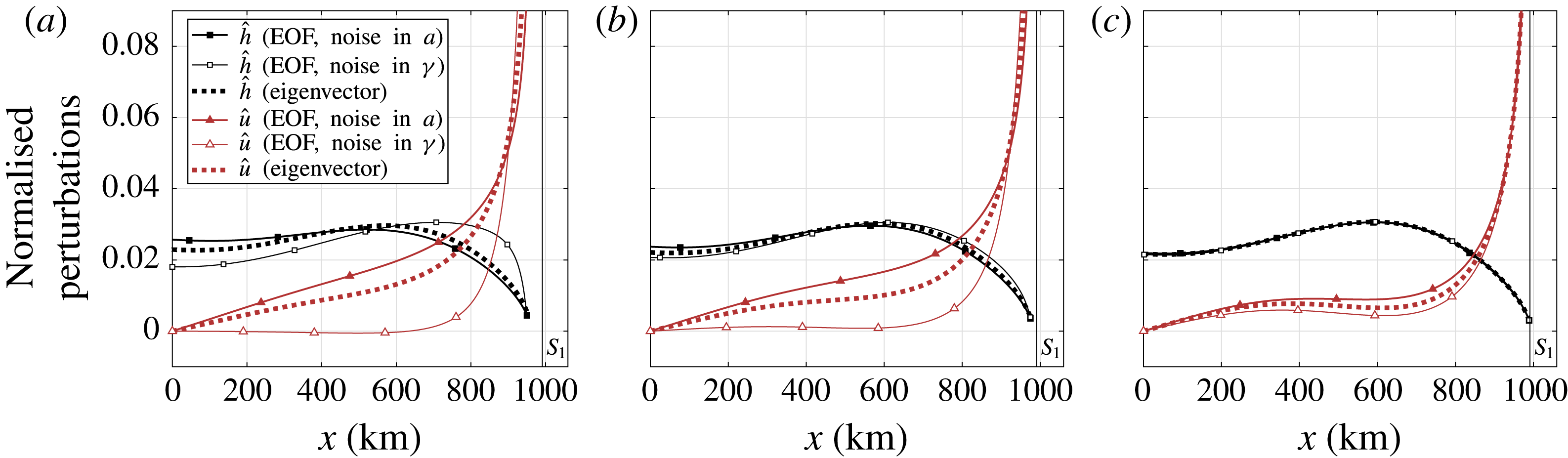
The first empirical orthogonal function (EOF), i.e. the dominant eigenvector corresponding to the rightmost eigenvalue of the covariance matrix, is shown in figure 7 (closed markers) for three stable equilibria with their grounding line at points
 $P_{1}=40.96~\text{km}$
,
 $P_{2}=16.384~\text{km}$
and
 $P_{3}=2048~\text{m}$
to the left of the grounding line position at
 $S_{1}$
. Noise is added to the accumulation with standard deviation
 $\unicode[STIX]{x1D702}_{ac}=\bar{a}/10~\text{my}^{-1}$
. The position of the equilibria and the explained variance of the EOFs are given in table 3. In the case of noise in accumulation, the EOFs correspond very well to the eigenvectors of the linear stability problem (dotted in figure 7).
First empirical orthogonal functions (EOF) for grounding lines at points
 $P_{1}$
(left),
 $P_{2}$
(centre) and
 $P_{3}$
(right) to the left of the first saddle-node bifurcation
 $S_{1}$
, together with the dominant eigenvector of the Jacobian matrix corresponding to the rightmost eigenvalue (dotted). Noise is added to the uniform accumulation with standard deviation
 $\unicode[STIX]{x1D702}_{ac}=\bar{a}/10~\text{my}^{-1}$
(closed markers) or to the sea level at the grounding line with
 $\unicode[STIX]{x1D702}_{sl}=1~\text{m}$
(open markers). The separate components corresponding to thickness (black squares) and velocity (red triangles) are normalised and their sign is taken according to a positive grounding line perturbation
 $\tilde{x}_{g}>0$
. The explained variances of the EOFs at
 $P_{1}$
,
 $P_{2}$
and
 $P_{3}$
are given in table 3.
Horizontal position of the points
 $P_{1}$
,
 $P_{2}$
and
 $P_{3}$
. The grounding line at the bifurcation
 $S_{1}$
is positioned at 991.261 km from the origin. The explained variance (scaled rightmost eigenvalue) corresponding to each EOF,
 $\unicode[STIX]{x1D70E}_{expl}^{2}$
, is given for noise in accumulation and noise in sea level (see also figure 8).

4.2 Additive noise in sea level
Another source of variability is the sea level at the grounding line
 $S(x_{g})$
. In the model, the sea level enters through the flotation condition (2.5). Adding noise to the sea level gives a system of SDAEs, where the stochastic forcing appears in the algebraic constraints. Using the transformation
 $\tilde{\boldsymbol{x}}=R\boldsymbol{z}$
and again combining the algebraic constraints, we find:
 $$\begin{eqnarray}\displaystyle \left[\begin{array}{@{}cc@{}}\unicode[STIX]{x1D644} & 0\\ 0 & 0\end{array}\right]\left[\begin{array}{@{}c@{}}\text{d}\boldsymbol{z}_{1}\\ \text{d}\boldsymbol{z}_{2}\end{array}\right]=\left[\begin{array}{@{}cc@{}}\unicode[STIX]{x1D645}_{11} & \unicode[STIX]{x1D645}_{12}\\ \unicode[STIX]{x1D645}_{21} & \unicode[STIX]{x1D645}_{22}\end{array}\right]\unicode[STIX]{x1D64D}\left[\begin{array}{@{}c@{}}\boldsymbol{z}_{1}\\ \boldsymbol{ z}_{2}\end{array}\right]\text{d}t+\left[\begin{array}{@{}c@{}}0\\ B_{s}\end{array}\right]\text{d}\boldsymbol{W}. & & \displaystyle\end{eqnarray}$$
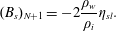
The noise forcing now enters through the flotation condition and is determined via
 $B_{s}\in \mathbb{R}^{(N+1)}$
, with elements
 $$\begin{eqnarray}\displaystyle & \displaystyle (B_{s})_{i}=0,\quad i=1,\ldots ,N-1, & \displaystyle\end{eqnarray}$$
 $$\begin{eqnarray}\displaystyle & \displaystyle (B_{s})_{N}=-\frac{1}{2}\left(1-{\displaystyle \frac{\unicode[STIX]{x1D70C}_{i}}{\unicode[STIX]{x1D70C}_{w}}}\right)\unicode[STIX]{x1D70C}_{w}g\unicode[STIX]{x1D702}_{sl}, & \displaystyle\end{eqnarray}$$
 $$\begin{eqnarray}\displaystyle & \displaystyle (B_{s})_{N+1}=-2\frac{\unicode[STIX]{x1D70C}_{w}}{\unicode[STIX]{x1D70C}_{i}}\unicode[STIX]{x1D702}_{sl}. & \displaystyle\end{eqnarray}$$
The final two entries of
 $B_{s}$
follow directly from incorporating sea level noise in the two discretised right boundary conditions in appendix A, specifically (A 23) and (A 24), where the stochastic terms are separated to give the entries in
 $B_{s}$
. Eliminating
 $\boldsymbol{z}_{2}$
gives an OU-process in
 $\boldsymbol{z}_{1}$
:
 $$\begin{eqnarray}\displaystyle & \displaystyle \text{d}\boldsymbol{z}_{1}=\unicode[STIX]{x1D651}\boldsymbol{z}_{1}\,\text{d}t+\tilde{B}_{s}\,\text{d}\boldsymbol{W},\quad \text{with}~\unicode[STIX]{x1D651}=\tilde{\unicode[STIX]{x1D645}}_{11}-\tilde{\unicode[STIX]{x1D645}}_{12}\tilde{\unicode[STIX]{x1D645}}_{22}^{-1}\tilde{\unicode[STIX]{x1D645}}_{21},\tilde{B}_{s}=-\tilde{\unicode[STIX]{x1D645}}_{12}\tilde{\unicode[STIX]{x1D645}}_{22}^{-1}B_{s}. & \displaystyle\end{eqnarray}$$
The covariance matrix of the perturbation
 $\tilde{\boldsymbol{x}}$
is subsequently found by solving
 $$\begin{eqnarray}\displaystyle & \displaystyle \unicode[STIX]{x1D651}\unicode[STIX]{x1D655}_{11}+\unicode[STIX]{x1D655}_{11}V^{\text{T}}+\tilde{B}_{s}\tilde{B}_{s}^{\text{T}}=0, & \displaystyle\end{eqnarray}$$
computing the remaining blocks in
 $\unicode[STIX]{x1D655}$
using the algebraic constraints in (4.7) and computing
 $\unicode[STIX]{x1D63E}=\unicode[STIX]{x1D64D}\unicode[STIX]{x1D655}\unicode[STIX]{x1D64D}^{\text{T}}$
. The first EOF is plotted in figure 7 (open markers), again for stable equilibria at
 $P_{1}$
,
 $P_{2}$
and
 $P_{3}$
. The standard deviation for noise in sea level is taken
 $\unicode[STIX]{x1D702}_{sl}=1~\text{m}$
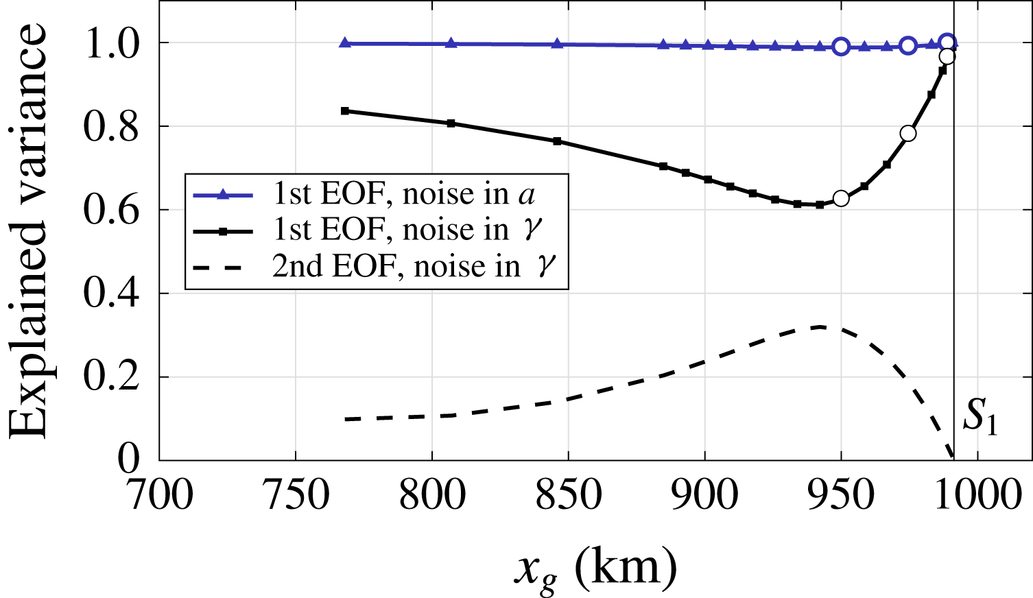
. For each EOF in figure 7, the corresponding explained variance is given by the solid lines in figure 8. An additional (dashed) eigenvalue curve in figure 8 shows the explained variance of the second dominant EOF for sea level noise.
Explained variance of EOFs due to noise in accumulation and sea level, i.e. rightmost eigenvalues of the covariance matrices, scaled with the total sum of the eigenvalues (trace). The open circles mark the points
 $P_{1}$
,
 $P_{2}$
,
 $P_{3}$
from left to right. Two eigenvalues are plotted for noise in sea level, as the variability is influenced by a second mode to the left of the first bifurcation
 $S_{1}$
.
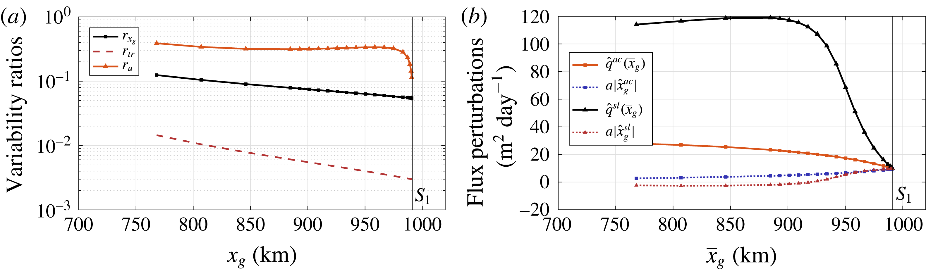
(a) Ratio of the grounding line standard deviation due to noise in sea level
 $\unicode[STIX]{x1D70E}_{x_{g}}^{sl}$
and noise in accumulation rate
 $\unicode[STIX]{x1D70E}_{x_{g}}^{ac}$
, for several points along the branch before the first saddle-node bifurcation
 $S_{1}$
. The noise amplitudes are
 $\unicode[STIX]{x1D702}_{ac}=\bar{a}/10~\text{my}^{-1}$
and
 $\unicode[STIX]{x1D702}_{sl}=1~\text{m}$
. Ratios of the total variability and the ratios for velocity variability at the grounding line are plotted as well. (b) Flux perturbations at the steady grounding line, computed from the first EOF for both noise in accumulation rate and noise in sea level at several points along the branch before the first bifurcation.
The structure of the sea level noise induced EOFs is noticeably different from the eigenvector patterns of the Jacobian matrix, in particular at points
 $P_{1}$
and
 $P_{2}$
(left and centre panel in figure 7). Overall, the explained variance of the dominant EOF at the three positions is considerably less than in the accumulation case. The difference between the EOFs of both noise types is due to the spatial noise distribution in the Ornstein–Uhlenbeck process. The noise in accumulation is distributed homogeneously, whereas the noise in sea level is applied with a spatial pattern given by
 $-\tilde{\unicode[STIX]{x1D645}}_{12}\tilde{\unicode[STIX]{x1D645}}_{22}^{-1}B_{s}$
. With this spatial pattern a second EOF is excited that competes with the dominant EOF before the bifurcation, see figure 8.
4.3 Unique regime: stochastic variability
With the availability of covariance matrices at any stable steady state, we can investigate the effect of the two distinct noise sources on the grounding line variability. In figure 9(a), we plot the ratio of the grounding line standard deviations
 $\unicode[STIX]{x1D70E}_{x_{g}}$
due to noise in sea level and accumulation rate:
 $$\begin{eqnarray}\displaystyle r_{x_{g}}=\unicode[STIX]{x1D70E}_{x_{g}}^{sl}/\unicode[STIX]{x1D70E}_{x_{g}}^{ac}. & & \displaystyle\end{eqnarray}$$
Next to the grounding line noise response, we are interested in the total induced variability and hence depict the ratio of the covariance matrix traces
 $$\begin{eqnarray}\displaystyle r_{tr}=\mathop{\sum }_{i}(\unicode[STIX]{x1D70E}_{i}^{sl})^{2}/\mathop{\sum }_{i}(\unicode[STIX]{x1D70E}_{i}^{ac})^{2},\quad i=1,\ldots ,2N+1, & & \displaystyle\end{eqnarray}$$
where
 $\unicode[STIX]{x1D70E}_{i}^{2}$
is the dimensional variance of every state vector component. The ratio of the velocity standard deviations at the grounding line are given as well:
 $$\begin{eqnarray}\displaystyle r_{u}=\unicode[STIX]{x1D70E}_{u_{N}}^{sl}/\unicode[STIX]{x1D70E}_{u_{N}}^{ac}. & & \displaystyle\end{eqnarray}$$
The quantities are plotted along the bifurcation diagram up to the saddle-node bifurcation
 $S_{1}$
. For our amplitude choices
 $\unicode[STIX]{x1D702}_{ac}$
,
 $\unicode[STIX]{x1D702}_{sl}$
, the effect of noise in the accumulation rate on the variability in the grounding line position is considerably greater than that due to sea level noise, in agreement with the analysis in Hogg et al. (Reference Hogg, Shepherd, Gourmelen and Engdahl2016). In the vicinity of the saddle-node bifurcation, the ratio
 $r_{u}$
shows a local maximum due to sea level variability. As the total dimensional variability is mainly determined by the grounding line variance, the effect is not present in the ratio
 $r_{tr}$
.
The noise induced perturbations in grounding line flux and accumulation are computed from the relevant EOFs and plotted in figure 9(b). The sea level induced maximum in
 $r_{u}$
is related to the difference in noise induced flux perturbations
 $\hat{q}(x_{g})$
, which directly depend on the ice thickness at the grounding line. The flux perturbation under sea level variability
 $\hat{q}^{sl}(x_{g})$
remains large, close to the bifurcation, compared to its accumulation counterpart
 $\hat{q}^{ac}(x_{g})$
.
Note that the fluxes calculated from the EOF due to noise in accumulation mimic the perturbations in figure 6(b), since this mode follows the eigenvectors of the Jacobian matrix. Furthermore, analogous to the results in figures 5 and 6(b) and Schoof (Reference Schoof2007a ), we find that, at the bifurcation, the noise induced accumulation and grounding line flux perturbations behave according to the instability mechanism (Schoof Reference Schoof2012), with equality at the bifurcation.
Recall that figure 6 shows a significant change in the multiple equilibria regime when a GSLE is represented in the model. Using the Lyapunov techniques described in the previous section we can now investigate the stochastic properties of the different model configurations. For every computed stable point in the bifurcation diagram we solve the Lyapunov equation and determine the variances for noise in the accumulation rate and noise in the sea level variability. The results are shown in figures 10 and 11.
Comparison of the model statistics without (black) and with a gravitational sea level effect GSLE (red), with additive noise in the accumulation. (a) Grounding line standard deviation
 $\unicode[STIX]{x1D70E}_{x_{g}}$
at every stable point in the bifurcation diagram, where
 $L_{1},S_{1}$
and
 $L_{2},S_{2}$
mark the first and second bifurcation encountered when decreasing
 $A$
. (b) Grounding line flux standard deviation
 $\unicode[STIX]{x1D70E}_{uh}$
. (c) Overlay of the data in (a), such that the bifurcation points lie on the dashed line. (d) Overlay of the data in (b).
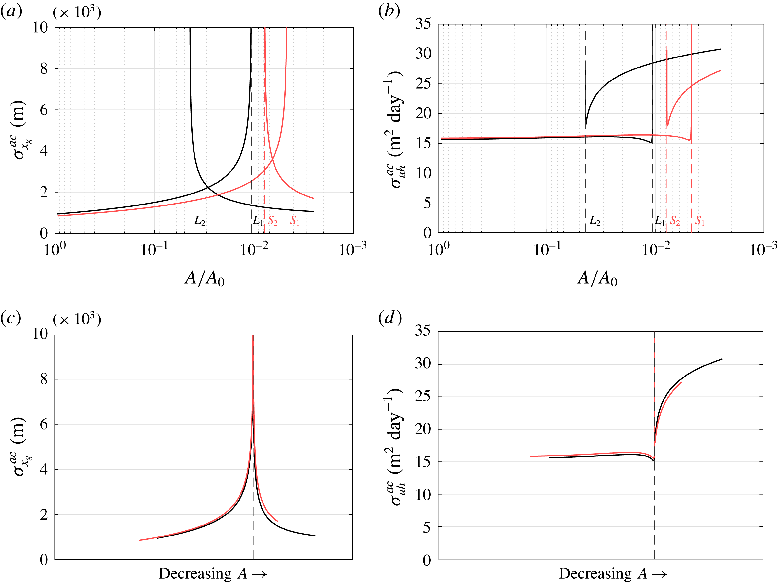
The introduction of a sea level equation causes a slight change in the stochastic properties under noise in accumulation rate. In general, as the multiple equilibria regime is shifted and decreased, an ice sheet will have a smaller grounding line variance and grounding line position for the same parameter value
 $A$
(cf. figure 6). Hence, the adaptation of the effective topographic slope causes the sheet to become more resilient under noise.
The standard deviations of the grounding line flux shown in figures 10(b) and 10(d) are computed from
 $$\begin{eqnarray}\displaystyle \displaystyle \unicode[STIX]{x1D70E}_{uh}^{2}=\text{Var}(uh) & = & \displaystyle \text{Var}((\bar{u}+\tilde{u} )(\bar{h}+\tilde{h}))\end{eqnarray}$$
 $$\begin{eqnarray}\displaystyle & {\approx} & \displaystyle \bar{h}^{2}~\text{Var}(\tilde{u} )+\bar{u}^{2}~\text{Var}(\tilde{h})+2\bar{h}\bar{u}~\text{Cov}(\tilde{u} ,\tilde{h}),\end{eqnarray}$$
where we distinguish between steady (
 $\bar{u},\bar{h}$
) and stochastic components (
 $\tilde{u} ,\tilde{h}$
), and ignore higher-order terms. The variability in flux shows a decrease just before a bifurcation, followed by a drastic increase at the bifurcations. This in contrast to the grounding line variability, which shows a steady increase when approaching a bifurcation. The overlay of the bifurcations in figure 10(c,d) shows a lack of qualitative differences in the stochastic properties. However, for both model configurations we find a major asymmetry in the flux variability around the bifurcations, a feature that is not present in the grounding line variability.
Comparison of the model statistics without (black) and with a gravitational sea level effect GSLE (red), with additive noise at the sea level. (a) Standard deviation
 $\unicode[STIX]{x1D70E}_{x_{g}}$
at every stable point in the bifurcation diagram, where
 $L_{1},S_{1}$
and
 $L_{2},S_{2}$
denote the first and second bifurcation encountered when decreasing
 $A$
. (b) Standard deviation of the grounding line flux
 $\unicode[STIX]{x1D70E}_{uh}$
. (c) Overlay of the data in (a), the bifurcations lie on the dashed line. (d) Overlay of the data in (b).
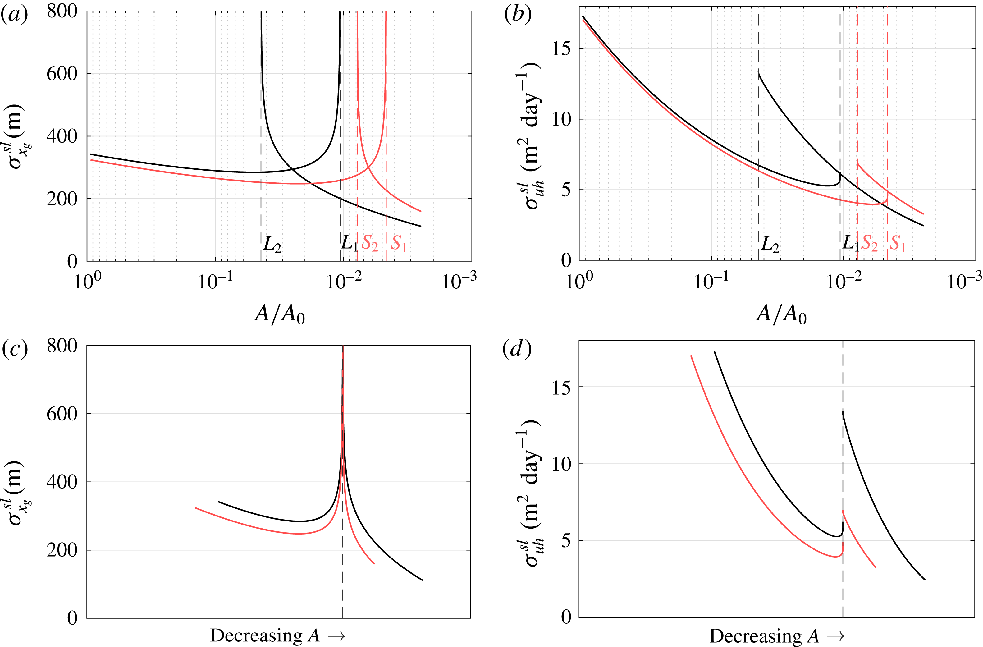
The difference in variances between the models with the two different sea level representations in the case of noise in sea level are more pronounced. Both grounding line and flux variance show a decreasing trend as the sheet becomes larger under decreasing
 $A$
, see figures 11(a) and 11(b). An ice sheet will vary less under sea level noise as its size increases. The overlays in figures 11(c) and 11(d) show that the adaptation of the effective topographic slope causes a significant additional damping, which cannot be solely due to a difference in sheet size, since at
 $A/A_{0}\sim 1$
the sheets are equal in size for both model configurations. As noise in sea level is applied at the grounding line, the model response is likely to be more sensitive to changes in slope than the response to noise in accumulation. Note that, again, an asymmetry is present in the flux variability.
In general, the results in figures 10 and 11 show typical grounding line variabilities ranging from
 $\mathit{O}(100~\text{m})$
for noise in sea level, to
 $\mathit{O}(1000~\text{m})$
for noise in accumulation, depending on the dynamical regime. A continuation of steady states accompanied by the solution of the Lyapunov equations enables a straightforward separation of variability sources. This may be useful to explain observed grounding line migration (Hogg et al.
Reference Hogg, Shepherd, Gourmelen and Engdahl2016), as will be elaborated in the discussion below.
4.4 Multiple equilibria: transition probabilities
For noise in accumulation we find roughly the same variability with a GSLE equation as in the case without such a representation. In contrast, variability due to noise in sea level is clearly dampened by the added GSLE equation. Here, the adaptation of the topographic slope appears to not only dampen the growth of perturbations, but also reduce the spread of the probability distributions along the branch. In figure 6, however, the distance between the stable branches is reduced in the GSLE configuration. This could have an effect on noise induced transitions in the multiple equilibrium regime, which we will investigate in this section. Although there is less sea level induced variability in the GSLE configuration, a smaller spatial distance between high (
 $2N+1$
) dimensional ellipsoidal confidence regions may indicate higher transition probabilities (Kuehn Reference Kuehn2012).
These confidence ellipsoids are determined by the probability density functions (PDFs) and indicate, with a certain confidence, where a state may be during a transient computation. The distance between ellipsoids associated with equilibria at different branches, but with the same parameter value, provides information about the relative frequency of noise induced transitions (Kuehn Reference Kuehn2012). Hence, calculating the distance between ellipsoids can be worthwhile when transient computations are expensive. Note, however, that such confidence regions are limited to representing the PDF under the assumption of linearised dynamics according to (2.22). For more information about these ellipsoids, see for instance Cowan (Reference Cowan1998).
Assuming we have computed a stable deterministic steady state
 $(\bar{\boldsymbol{x}},A)$
and the associated covariance matrix
 $\unicode[STIX]{x1D63E}$
, then the confidence ellipsoid can be represented as
 $$\begin{eqnarray}\displaystyle & \displaystyle E=\big\{\boldsymbol{x}\in \mathbb{R}^{2N+1}:\boldsymbol{v}^{\text{T}}\boldsymbol{x}\leqslant \boldsymbol{v}^{\text{T}}\bar{\boldsymbol{x}}+\sqrt{\boldsymbol{v}^{\text{T}}\tilde{\unicode[STIX]{x1D63E}}\boldsymbol{ v}}~\forall ~\boldsymbol{v}\in \mathbb{R}^{2N+1}\big\}, & \displaystyle\end{eqnarray}$$
where
 $\tilde{\unicode[STIX]{x1D63E}}=Q_{\unicode[STIX]{x1D6FC}}\unicode[STIX]{x1D63E}$
is the positive semi-definite shape matrix associated with the confidence ellipsoid and
 $Q_{\unicode[STIX]{x1D6FC}}=3239$
is a scalar that can be obtained from the
 $\unicode[STIX]{x1D712}^{2}$
-distribution for a confidence level
 $1-\unicode[STIX]{x1D6FC}=0.683$
(Cowan Reference Cowan1998).
To determine the distance
 $d$
between ellipsoids, a convex minimisation problem of the form
 $$\begin{eqnarray}\displaystyle & \displaystyle -d=\min _{\Vert \boldsymbol{v}\Vert _{2}=1}\left(-\boldsymbol{v}^{\text{T}}\bar{\boldsymbol{x}}_{1}+\sqrt{\boldsymbol{v}^{\text{T}}\tilde{\unicode[STIX]{x1D63E}_{1}}\boldsymbol{ v}}+\boldsymbol{v}^{\text{T}}\bar{\boldsymbol{x}}_{2}+\sqrt{\boldsymbol{v}^{\text{T}}\tilde{\unicode[STIX]{x1D63E}_{2}}\boldsymbol{ v}}\right) & \displaystyle\end{eqnarray}$$
is solved. Here
 $\bar{\boldsymbol{x}}_{1}$
is an equilibrium at one branch and
 $\bar{\boldsymbol{x}}_{2}$
the equilibrium at the other branch, for the same parameter value
 $A$
.
 $\tilde{\unicode[STIX]{x1D63E}_{1}}=Q_{\unicode[STIX]{x1D6FC}}\unicode[STIX]{x1D63E}_{1}$
and
 $\tilde{\unicode[STIX]{x1D63E}_{2}}=Q_{\unicode[STIX]{x1D6FC}}\unicode[STIX]{x1D63E}_{2}$
are the respective shape matrices.
Distance patterns between the ellipsoids, calculated for the case without GSLE (black) and the case with GSLE (red), for noise at the accumulation (solid line) and at the sea level (dashed line). The noise amplitudes for the different sources (
 $\unicode[STIX]{x1D702}_{ac}$
,
 $\unicode[STIX]{x1D702}_{sl}$
) are amplified according to the amplifications in the transient results (see figure 13).
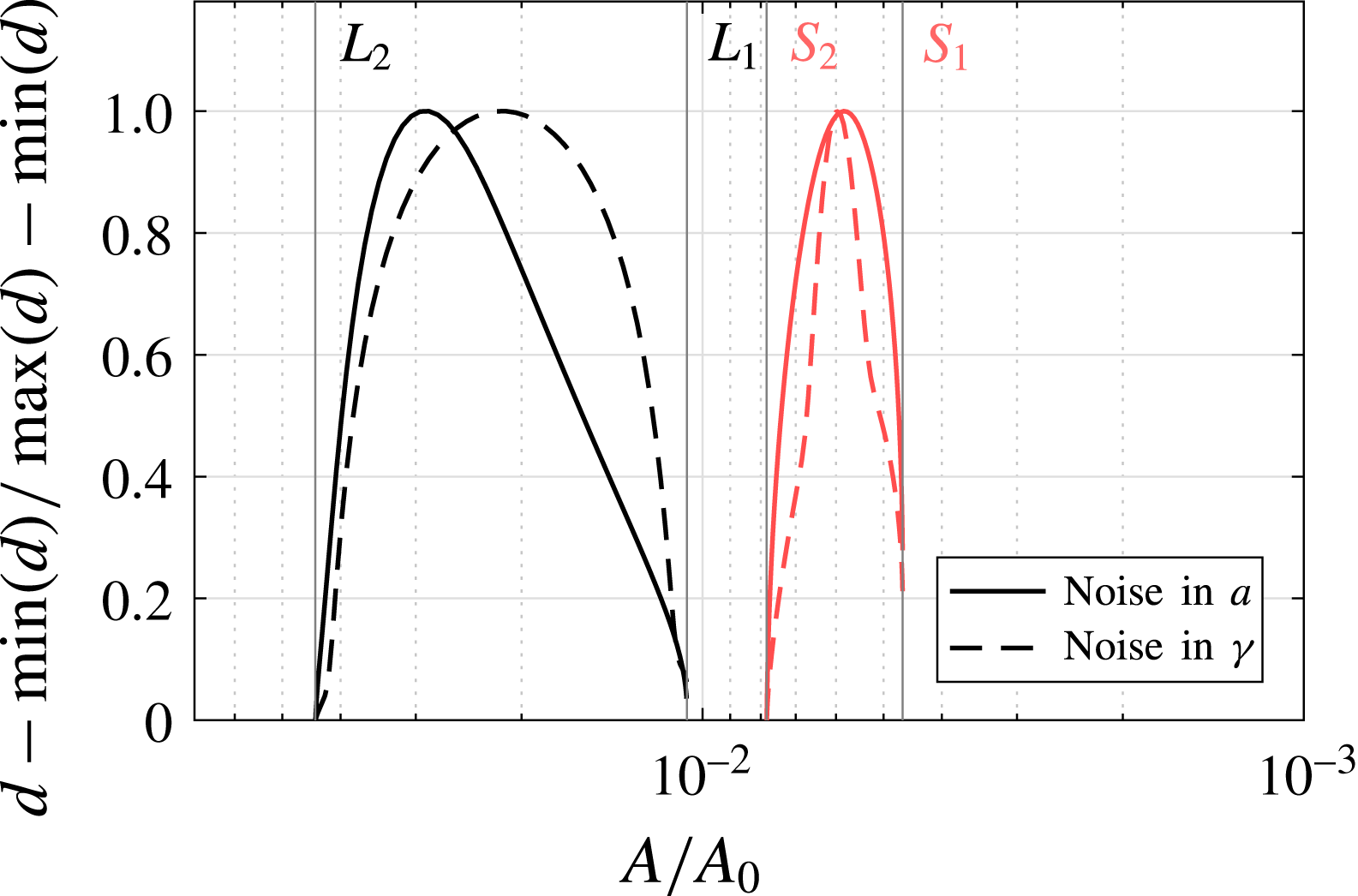
The results in figure 12 show that the distance between the ellipsoids is clearly reduced when approaching a bifurcation point, leading to larger transition probabilities (Kuehn Reference Kuehn2012). The shapes of the distances reveal asymmetries between the bifurcations. The case without GSLE shows a slight minimum at
 $L_{2}$
. The case with GSLE has a similar, but more pronounced asymmetry with a minimum distance at
 $S_{2}$
.
The main drawback of the ellipsoid distance computation is that it is based on local dynamical and stochastic behaviour of the model, combined with the global distance between branches. Possible nonlinear processes that affect the noise induced perturbations are, at best, only partially represented. Moreover, to compare the different model configurations, we restrict ourselves to normalised distance patterns in figure 12. Actual distance values have little meaning and serve merely as a test function for transition probabilities (Kuehn Reference Kuehn2012).
To verify the relative transition frequencies that the ellipsoid distances in figure 12 suggest, we perform transient computations using a backward Euler–Maruyama scheme, a well-established time integration technique for systems of SDAEs. Here, the deterministic part of (2.12) is treated implicitly, whereas the stochastic part is integrated explicitly with respect to a Brownian path. For a transition count we define a transition as a trajectory
 $\unicode[STIX]{x1D703}(t)$
from the upper branch to the lower branch and vice versa, similar to the definition in Kuehn (Reference Kuehn2012). Let
 $\boldsymbol{p}^{u}$
and
 $\boldsymbol{p}^{l}$
denote steady states in the upper and lower branch respectively and define some small tolerance
 $\unicode[STIX]{x1D70C}$
. A trajectory is counted as a transition from the upper to the lower branch
 $T^{u\rightarrow l}$
when it reaches a neighbourhood of
 $\boldsymbol{p}^{l}$
,
 $||\unicode[STIX]{x1D703}(t)-\boldsymbol{p}^{l}||_{2}<\unicode[STIX]{x1D70C}$
, after visiting a neighbourhood of
 $\boldsymbol{p}^{u}$
,
 $||\unicode[STIX]{x1D703}(t)-\boldsymbol{p}^{u}||_{2}<\unicode[STIX]{x1D70C}$
, within some time
 $T_{e}$
.
 $T^{l\rightarrow u}$
is defined similarly. In order to get a reliable number of transitions, we need to multiply the standard deviations
 $\unicode[STIX]{x1D702}_{ac},\unicode[STIX]{x1D702}_{sl}$
by amplification factors
 $f_{ac},f_{sl}$
, respectively. In the case of noise in the accumulation we choose
 $f_{ac}=5$
, for the sea level noise we choose
 $f_{sl}=20$
. The results are shown in figures 13(a) and 13(b).
Sum of the transitions from the upper to the lower branch and vice versa, relative to the total number of transients
 $N_{trans}$
, i.e.
 $(\#T^{u\rightarrow l}+\#T^{l\rightarrow u})/N_{trans}$
. (a) Transitions under noise in accumulation with GSLE (red) and without GSLE (black), using a backward Euler–Maruyama time integration with time step
 $\unicode[STIX]{x0394}t=1000~y$
, end time
 $T_{e}=100\,000~y$
and amplified standard deviation
 $f_{ac}\unicode[STIX]{x1D702}_{ac}$
,
 $f_{ac}=5$
. (b) Transitions under noise in sea level with GSLE (red) and without GSLE (black), with amplified noise
 $f_{sl}\unicode[STIX]{x1D702}_{sl}$
,
 $f_{sl}=20$
. The total number of transient experiments for each point on the branch is
 $N_{trans}=960$
. A neighbourhood is defined in terms of grounding line positions, where the tolerance is chosen to be
 $\unicode[STIX]{x1D70C}=10~\text{km}$
.
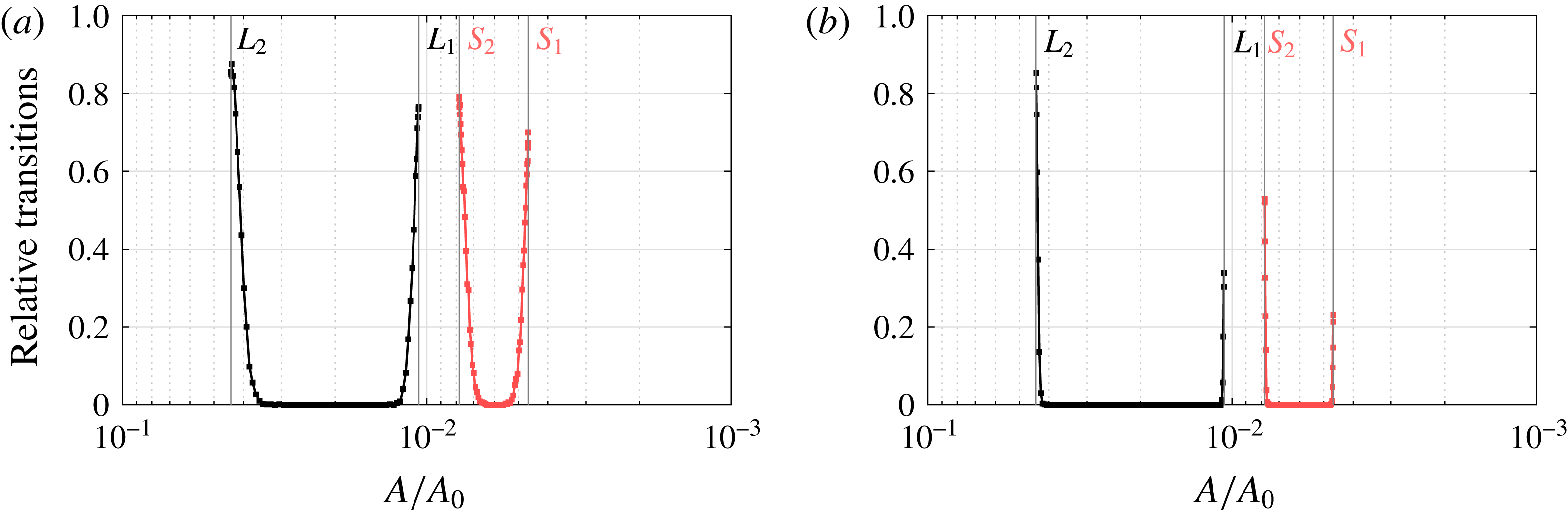
Although the distance between the probability distributions shows a decrease, this is not sufficient to compensate for the decrease in variability. Hence, the number of transitions is significantly reduced in the model with GSLE. This holds for both noise in accumulation rate (figure 13 a) and noise in sea level (figure 13 b), although the reduction of variability is more drastic in the sea level noise case.
From the results in figure 13 we may conclude that it is more likely to travel from the upper branch (large sheet) to the lower branch (small sheet) than vice versa, which holds for both noise types. The asymmetry in figure 12 for both model configurations is similar. As described above, the same asymmetry can be found in the flux variability. Figures 10(d) and 11(d) show that the flux variability near
 $L_{2}(S_{2})$
at the upper branch is generally higher than at the lower branch near
 $L_{1}(S_{1})$
, which is likely due to the weaker effective topographical slope at
 $L_{2}(S_{2})$
.
5 Summary and discussion
Even dynamically stable marine ice sheets display substantial variability in their grounding lines (Hogg et al.
Reference Hogg, Shepherd, Gourmelen and Engdahl2016). In this paper, we have investigated the stochastic variability of marine ice sheets in a two-dimensional model with a specific bed topography (Schoof Reference Schoof2007a
). The deterministic model already has an interesting behaviour with unique regimes and a multiple equilibrium regime. The back-to-back saddle-node bifurcation diagram is associated with the traditional stationary marine ice sheet instability (Schoof Reference Schoof2012). The changes in the parameter
 $A$
in Glen’s flow law, used as control parameter, are interpreted here as changes in external conditions such as the mean atmospheric temperature over the ice sheet.
As far as we know this is the first study where the bifurcation diagrams of such two-dimensional marine ice sheet models have been explicitly computed using continuation methods. The continuation approach allows the computation of eigenvectors of the steady states in the multiple equilibrium regime, at both stable and unstable branches. With this information it was possible to validate and extend findings based on the boundary layer theory in Schoof (Reference Schoof2007a
) and Schoof (Reference Schoof2012). In figure 4(d), for instance, the eigenvectors at the unstable branch confirm the mechanism at the grounding line as explained in Schoof (Reference Schoof2007a
), but also reveal the associated behaviour in the interior of the ice sheet. A positive eigenvalue was shown to be associated with the instability criterion (Schoof Reference Schoof2012) for the full problem. The advected thickness perturbation (the term
 $\bar{u}{\hat{h}}$
, where
 $\bar{u}$
is the steady state velocity and
 ${\hat{h}}$
the ice thickness perturbation) turns out to dominate the instability process.
We also showed that the representation of the gravitational sea level effect as used in Gomez et al. (Reference Gomez, Mitrovica, Huybers and Clark2010) leads only to a shift in the bifurcation diagram and a slight decrease in the width of the hysteresis characterising the multiple equilibrium regime. From this perspective, it does not add any new dynamics to the marine ice sheet system, but only quantitatively modifies the stability properties of the states. The mechanism of destabilisation is also similar to that of the flat sea level case and the growth of perturbations can be connected to an ‘effective’ topography slope.
The main innovation in this work, however, is the analysis of the response of the marine ice sheet to small amplitude stochastic noise in accumulation rate and sea level. Under linearised dynamics of the perturbations, the covariance matrix can be determined from a Lyapunov equation that was solved efficiently using the RAILS method (Baars et al. Reference Baars, Viebahn, Mulder, Kuehn, Wubs and Dijkstra2017). Here we have restricted our analysis to additive noise, but elaborate accumulation noise distributions are easily studied using the Lyapunov approach. In the unique regime of the ice sheet, it is found that the variability induced by the sea level noise is much smaller than that due to the accumulation rate. The order of magnitude (for typical noise levels) is of the order of 100 m grounding line variations for sea level noise and 1000 m for noise in the accumulation.
There are only very limited data available on grounding line migration (e.g. 19 years in Hogg et al. (Reference Hogg, Shepherd, Gourmelen and Engdahl2016)). In addition, the two-dimensional model here is highly idealised, with only one bed topography and also one particular parameterisation to represent the gravitational effect on sea level. Hence, only a qualitative comparison between the model results and observations can be made. Our results indicate that accumulation noise can induce grounding line excursions of the observed magnitude and that noise in sea level variations plays only a minor role, in agreement with the analysis in Hogg et al. (Reference Hogg, Shepherd, Gourmelen and Engdahl2016).
One important effect that has been neglected in the analysis of this paper is that of buttressing, i.e. stresses exerted on the ice sheet due to floating ice. The reason is that, in the two-dimensional model context, such an ice-shelf buttressing effect is absent (Gudmundsson Reference Gudmundsson2012). However, in reality (and in three-dimensional models), this effect can clearly be important. To estimate the magnitude of buttressing effects within our model context, we propose a stochastic parameterisation of these inherently three-dimensional effects in appendix E. The results in appendix E show that grounding line variations of the order of 1000 m are already obtained for a buttressing variability of 2 % of the full stress regime (from fully buttressed to unbuttressed). Hence, short-term variations in ice thickness and variations in ice-shelf buttressing may both play an important role in real grounding line migrations (Hogg et al. Reference Hogg, Shepherd, Gourmelen and Engdahl2016). As ice-shelf break-up may give a change of up to 100 % of the stress regime, a standard deviation of 2 % is not unthinkable. It is thus necessary to find a realistic estimate of temporal buttressing variability using, for instance, the approach in Fürst et al. (Reference Fürst, Durand, Gillet-Chaulet, Tavard, Rankl, Braun and Gagliardini2016). Future work could then use the Lyapunov approach to further extend the comparison of the effect of noise sources on grounding line variability.
Having determined the extent of the equilibrium regime, we studied the transition probabilities between both states using transient simulations and distances between confidence ellipsoids. We find that, for both accumulation and sea level noise types, it is more likely to jump from a large ice sheet state to a small ice sheet state than vice versa. Grounding line flux variability shows a related asymmetry, likely due to differences in local bedrock slope and/or global ice sheet extent. Although more work is needed to study the robustness of these results to different bed topographies, it can be anticipated that the parameter range of the transition regime will depend only on the local ‘effective’ topographic slope at the grounding line. The possibility of stochastic induced transitions (in multiple equilibrium regimes of marine ice sheets) adds another aspect of possible rapid climate changes which may have occurred in the past and which may occur in the future.
Acknowledgements
We would like to thank H. Goelzer for insightful discussions. Furthermore, we would like to thank the two anonymous referees for their helpful and thorough reviews, which have improved the manuscript considerably. T.E.M. and H.A.D. acknowledge support by the Netherlands Earth System Science Centre (NESSC), financially supported by the Ministry of Education, Culture and Science (OCW), grant no. 024.002.001. S.B. and F.W.W. acknowledge support from the Mathematics of Planet Earth research program, project number 657.000.007, which is financed by the Netherlands Organisation for Scientific Research (NWO).
Appendix A. Non-dimensional equations and numerical implementation
A.1 Non-dimensional equations
The first difficulty one encounters is the unknown right boundary of the problem given by the grounding line position
 $x_{g}$
. As discussed in Schoof (Reference Schoof2007a
) and Vieli & Payne (Reference Vieli and Payne2005), a moving grid approach can be used to track
 $x_{g}$
. Using a transformation
 $z=x/x_{g}$
, we are able to map the original domain
 $x\in [0,x_{g}]$
onto the fixed domain
 $z\in [0,1]$
. As a result, the problem now has three unknowns:
 $h$
,
 $u$
and
 $x_{g}$
. The differential operators are transformed using the chain rule:
 $$\begin{eqnarray}\displaystyle & \displaystyle \frac{\unicode[STIX]{x2202}}{\unicode[STIX]{x2202}t}=\frac{\unicode[STIX]{x2202}}{\unicode[STIX]{x2202}\unicode[STIX]{x1D70F}}\frac{\unicode[STIX]{x2202}\unicode[STIX]{x1D70F}}{\unicode[STIX]{x2202}t}+\frac{\unicode[STIX]{x2202}}{\unicode[STIX]{x2202}z}\frac{\unicode[STIX]{x2202}z}{\unicode[STIX]{x2202}t}=\frac{\unicode[STIX]{x2202}}{\unicode[STIX]{x2202}\unicode[STIX]{x1D70F}}-\frac{z}{x_{g}}\frac{\text{d}x_{g}}{\text{d}t}\frac{\unicode[STIX]{x2202}}{\unicode[STIX]{x2202}z}, & \displaystyle\end{eqnarray}$$
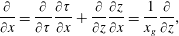 $$\begin{eqnarray}\displaystyle & \displaystyle \frac{\unicode[STIX]{x2202}}{\unicode[STIX]{x2202}x}=\frac{\unicode[STIX]{x2202}}{\unicode[STIX]{x2202}\unicode[STIX]{x1D70F}}\frac{\unicode[STIX]{x2202}\unicode[STIX]{x1D70F}}{\unicode[STIX]{x2202}x}+\frac{\unicode[STIX]{x2202}}{\unicode[STIX]{x2202}z}\frac{\unicode[STIX]{x2202}z}{\unicode[STIX]{x2202}x}=\frac{1}{x_{g}}\frac{\unicode[STIX]{x2202}}{\unicode[STIX]{x2202}z}, & \displaystyle\end{eqnarray}$$
where
 $z$
and
 $\unicode[STIX]{x1D70F}$
denote the independent variables in the transformed domain. Since we only transform in space we have that
 $\unicode[STIX]{x1D70F}=t$
. The transformations of (2.1)–(2.5) are given by (A 3)–(A 7):
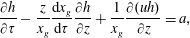 $$\begin{eqnarray}\displaystyle & \displaystyle \frac{\unicode[STIX]{x2202}h}{\unicode[STIX]{x2202}\unicode[STIX]{x1D70F}}-\frac{z}{x_{g}}\frac{\text{d}x_{g}}{\text{d}\unicode[STIX]{x1D70F}}\frac{\unicode[STIX]{x2202}h}{\unicode[STIX]{x2202}z}+\frac{1}{x_{g}}\frac{\unicode[STIX]{x2202}(uh)}{\unicode[STIX]{x2202}z}=a, & \displaystyle\end{eqnarray}$$
 $$\begin{eqnarray}\displaystyle & \displaystyle \frac{1}{x_{g}^{(1/n)+1}}\frac{\unicode[STIX]{x2202}}{\unicode[STIX]{x2202}z}\left[2A^{-1/n}h\left|\frac{\unicode[STIX]{x2202}u}{\unicode[STIX]{x2202}z}\right|^{1/n-1}\frac{\unicode[STIX]{x2202}u}{\unicode[STIX]{x2202}z}\right]-\unicode[STIX]{x1D63E}|u|^{(m-1)}u-\frac{\unicode[STIX]{x1D70C}_{i}gh}{x_{g}}\frac{\unicode[STIX]{x2202}(h-b)}{\unicode[STIX]{x2202}z}=0, & \displaystyle\end{eqnarray}$$
 $$\begin{eqnarray}\displaystyle & \displaystyle \frac{\unicode[STIX]{x2202}(h-b)}{\unicode[STIX]{x2202}z}=u=0\quad \text{for}~z=0, & \displaystyle\end{eqnarray}$$
 $$\begin{eqnarray}\displaystyle & \displaystyle \unicode[STIX]{x1D70C}_{i}h=\unicode[STIX]{x1D70C}_{w}(b+S)\quad \text{for}~z=1, & \displaystyle\end{eqnarray}$$
 $$\begin{eqnarray}\displaystyle & \displaystyle 2A^{-1/n}\frac{1}{x_{g}^{1/n}}\left|\frac{\unicode[STIX]{x2202}u}{\unicode[STIX]{x2202}z}\right|^{(1/n)-1}\frac{\unicode[STIX]{x2202}u}{\unicode[STIX]{x2202}z}=\frac{1}{2}\left(1-\frac{\unicode[STIX]{x1D70C}_{i}}{\unicode[STIX]{x1D70C}_{w}}\right)\unicode[STIX]{x1D70C}_{i}gh\quad \text{for}~z=1. & \displaystyle\end{eqnarray}$$
To improve numerical accuracy the equations are non-dimensionalised. Let
 $$\begin{eqnarray}\displaystyle h=h_{0}\tilde{h},\quad b=h_{0}\tilde{b},\quad S=h_{0}\tilde{S},\quad x_{g}=x_{0}\tilde{x}_{g},\quad u=u_{0}\tilde{u} ,\quad \unicode[STIX]{x1D70F}=\frac{x_{0}}{u_{0}}\tilde{\unicode[STIX]{x1D70F}}, & & \displaystyle\end{eqnarray}$$
with typical thickness
 $h_{0}=1\times 10^{3}~\text{m}$
, horizontal extent
 $x_{0}=1\times 10^{5}$
m and typical velocity
 $u_{0}=1~\text{m}~\text{day}^{-1}$
. Substituting these expressions in (A 3) gives
 $$\begin{eqnarray}\displaystyle & \displaystyle \frac{u_{0}h_{0}}{x_{0}}\left(\frac{\unicode[STIX]{x2202}\tilde{h}}{\unicode[STIX]{x2202}\tilde{\unicode[STIX]{x1D70F}}}-\frac{z}{\tilde{x}_{g}}\frac{\text{d}\tilde{x}_{g}}{\text{d}\tilde{\unicode[STIX]{x1D70F}}}\frac{\unicode[STIX]{x2202}\tilde{h}}{\unicode[STIX]{x2202}z}+\frac{1}{\tilde{x}_{g}}\frac{\unicode[STIX]{x2202}(\tilde{u} \tilde{h})}{\unicode[STIX]{x2202}z}\right)=a\Leftrightarrow \frac{\unicode[STIX]{x2202}\tilde{h}}{\unicode[STIX]{x2202}\tilde{\unicode[STIX]{x1D70F}}}-\frac{z}{\tilde{x}_{g}}\frac{\text{d}\tilde{x}_{g}}{\text{d}\tilde{\unicode[STIX]{x1D70F}}}\frac{\unicode[STIX]{x2202}\tilde{h}}{\unicode[STIX]{x2202}z}+\frac{1}{\tilde{x}_{g}}\frac{\unicode[STIX]{x2202}(\tilde{u} \tilde{h})}{\unicode[STIX]{x2202}z}=\tilde{a}, & \displaystyle\end{eqnarray}$$
with
 $\tilde{a}=x_{0}/u_{0}h_{0}a$
. Similarly, the non-dimensionalised version of (A 4) is given by
 $$\begin{eqnarray}\displaystyle \frac{c_{1}}{\tilde{x}_{g}^{(1/n)+1}}\frac{\unicode[STIX]{x2202}}{\unicode[STIX]{x2202}z}\left[2A^{-1/n}\tilde{h}\left|\frac{\unicode[STIX]{x2202}\tilde{u} }{\unicode[STIX]{x2202}z}\right|^{(1/n)-1}\frac{\unicode[STIX]{x2202}\tilde{u} }{\unicode[STIX]{x2202}z}\right]-c_{2}|\tilde{u} |^{(m-1)}\tilde{u} -c_{3}~\unicode[STIX]{x1D70C}_{i}g\frac{\tilde{h}}{\tilde{x}_{g}}\frac{\unicode[STIX]{x2202}(\tilde{h}-\tilde{b})}{\unicode[STIX]{x2202}z}=0, & & \displaystyle\end{eqnarray}$$
where we introduce new constants
 $$\begin{eqnarray}\displaystyle c_{1}=\frac{1}{C}\frac{h_{0}}{x_{0}}\left(\frac{u_{0}}{x_{0}}\right)^{1/n},\quad c_{2}=u_{0}^{m}\quad \text{and}\quad c_{3}=\frac{1}{C}\frac{h_{0}^{2}}{x_{0}}. & & \displaystyle\end{eqnarray}$$
Finally, at the boundaries we obtain
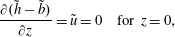 $$\begin{eqnarray}\displaystyle & \displaystyle \frac{\unicode[STIX]{x2202}(\tilde{h}-\tilde{b})}{\unicode[STIX]{x2202}z}=\tilde{u} =0\quad \text{for}~z=0, & \displaystyle\end{eqnarray}$$
 $$\begin{eqnarray}\displaystyle & \displaystyle \unicode[STIX]{x1D70C}_{i}\tilde{h}=\unicode[STIX]{x1D70C}_{w}\left(\tilde{b}+\tilde{S}\right)\quad \text{for}~z=1, & \displaystyle\end{eqnarray}$$
 $$\begin{eqnarray}\displaystyle & \displaystyle 2~c_{4}~A^{-1/n}\frac{1}{\tilde{x}_{g}^{1/n}}\left|\frac{\unicode[STIX]{x2202}\tilde{u} }{\unicode[STIX]{x2202}z}\right|^{(1/n)-1}\frac{\unicode[STIX]{x2202}\tilde{u} }{\unicode[STIX]{x2202}z}=\frac{1}{2}\left(1-\frac{\unicode[STIX]{x1D70C}_{i}}{\unicode[STIX]{x1D70C}_{w}}\right)\unicode[STIX]{x1D70C}_{i}g\tilde{h}\quad \text{for}~z=1, & \displaystyle\end{eqnarray}$$
with
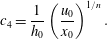 $$\begin{eqnarray}\displaystyle & \displaystyle c_{4}=\frac{1}{h_{0}}\left(\frac{u_{0}}{x_{0}}\right)^{1/n}. & \displaystyle\end{eqnarray}$$
A.2 Numerical implementation
From here on we omit the tildes and assume the unknowns are non-dimensional. As in Schoof (Reference Schoof2007a
), the domain
 $z\in [0,1]$
is discretised using a staggered grid with a fixed mesh-width:
 $\unicode[STIX]{x0394}z=1/(N-1/2)$
. The left boundary is taken at the vertex
 $i=1$
and the right boundary at the cell centre
 $i=N+1/2$
. Thus, for
 $i=1,2,\ldots ,N$
, we have vertices at
 $z_{i}=\unicode[STIX]{x0394}z(i-1)$
and cell centres at
 $z_{i+1/2}=\unicode[STIX]{x0394}z(i-1/2)$
. The discretised solution values for ice thickness are located at the vertices
 $h_{i}$
, while the values for ice velocity are positioned at the cell centres
 $u_{i+1/2}$
. Hence, the subscript
 $(i+1/2)$
denotes an existing location for the velocity unknowns.
The transformed and non-dimensionalised continuity equation (A 9) is discretised using a central difference for the stretching and an upwind discretisation for the flux:
 $$\begin{eqnarray}\displaystyle & \displaystyle \frac{\text{d}h_{i}}{\text{d}\unicode[STIX]{x1D70F}}-\frac{z_{i}}{x_{g}}\left(\frac{h_{i+1}-h_{i-1}}{2\unicode[STIX]{x0394}z}\right)\frac{\text{d}x_{g}}{\text{d}\unicode[STIX]{x1D70F}}=-\frac{h_{i}(u_{i+1/2}+u_{i-1/2})-h_{i-1}(u_{i-1/2}+u_{i-3/2})}{2x_{g}\unicode[STIX]{x0394}z}+a_{i}. & \displaystyle \nonumber\\ \displaystyle & & \displaystyle\end{eqnarray}$$
At the left boundary symmetry requires
 $$\begin{eqnarray}\displaystyle & \displaystyle (h_{2}-h_{0})/(2\unicode[STIX]{x0394}z)=0\quad \text{(central)}, & \displaystyle\end{eqnarray}$$
 $$\begin{eqnarray}\displaystyle & \displaystyle (h_{1}-h_{0})/\unicode[STIX]{x0394}z=0\quad \text{(upwind)}, & \displaystyle\end{eqnarray}$$
 $$\begin{eqnarray}\displaystyle & \displaystyle u_{3/2}+u_{1/2}=0,\quad u_{5/2}+u_{-1/2}=0. & \displaystyle\end{eqnarray}$$
Using these expressions we can resolve the dependence on the unknowns at non-existent grid points
 $h_{0},u_{-1/2},u_{1/2}$
. For
 $i=1$
and
 $i=2$
, mass conservation is therefore given by
 $$\begin{eqnarray}\displaystyle & \displaystyle (i=1)\quad \frac{\text{d}h_{1}}{\text{d}\unicode[STIX]{x1D70F}}=-\frac{h_{1}(u_{3/2}+u_{5/2})}{2x_{g}\unicode[STIX]{x0394}z}+a_{1}, & \displaystyle\end{eqnarray}$$
 $$\begin{eqnarray}\displaystyle & \displaystyle (i=2)\quad \frac{\text{d}h_{2}}{\text{d}\unicode[STIX]{x1D70F}}-\frac{z_{2}}{x_{g}}\left(\frac{h_{3}-h_{1}}{2\unicode[STIX]{x0394}z}\right)\frac{\text{d}x_{g}}{\text{d}\unicode[STIX]{x1D70F}}=-\frac{h_{2}(u_{5/2}+u_{3/2})}{2x_{g}\unicode[STIX]{x0394}z}+a_{2}. & \displaystyle\end{eqnarray}$$
Note that at the rightmost vertex (
 $i=N$
), the right-hand side of the discretised mass conservation (A 16) does not contain any dependencies on non-existent grid points. On the left-hand side we will need to use a one-sided difference for the stretching term.
Define
 $\unicode[STIX]{x0394}u_{i}:=u_{i+1/2}-u_{i-1/2}$
. The momentum conservation (A 10) is discretised using central differences:
 $$\begin{eqnarray}\displaystyle 0 & = & \displaystyle \frac{2~c_{1}~A^{-1/n}}{(x_{g}\unicode[STIX]{x0394}z)^{1+1/n}}\left[h_{i+1}|\unicode[STIX]{x0394}u_{i+1}|^{1/n-1}\unicode[STIX]{x0394}u_{i+1}-h_{i}|\unicode[STIX]{x0394}u_{i}|^{1/n-1}\unicode[STIX]{x0394}u_{i}\right]\nonumber\\ \displaystyle & & \displaystyle -\,c_{2}~{|u_{i+1/2}|}^{m-1}u_{i+1/2}-\left(\frac{h_{i}+h_{i+1}}{2}\right)\frac{c_{3}~\unicode[STIX]{x1D70C}_{i}g}{x_{g}\unicode[STIX]{x0394}z}[h_{i+1}-b_{i+1}-h_{i}+b_{i}].\end{eqnarray}$$
At the left boundary we let
 $\unicode[STIX]{x0394}u_{1}=2u_{3/2}$
. At the right boundary we impose the following discretisation of (A 14) with a substituted flotation condition
 $\unicode[STIX]{x1D70C}_{i}h_{N}=\unicode[STIX]{x1D70C}_{w}(b_{N}+S_{N})$
(cf. (A 13)):
 $$\begin{eqnarray}\displaystyle & \displaystyle 0=2A^{1/n}{\displaystyle \frac{c_{4}}{(x_{g}\unicode[STIX]{x0394}z)^{1/n}}}|\unicode[STIX]{x0394}u_{N}|^{1/n-1}(\unicode[STIX]{x0394}u_{N})-\frac{1}{2}\left(1-{\displaystyle \frac{\unicode[STIX]{x1D70C}_{i}}{\unicode[STIX]{x1D70C}_{w}}}\right)\unicode[STIX]{x1D70C}_{w}g(b_{N}+S_{N}). & \displaystyle\end{eqnarray}$$
The discretisation contains
 $N$
unknown
 $h_{i}$
,
 $N$
unknown
 $u_{i+1/2}$
and an unknown grounding line position
 $x_{g}$
. To achieve a closed system of
 $2N+1$
equations, the flotation criterion at the cell centre
 $z_{N+1/2}$
is prescribed using an extrapolation of the thickness, which gives the closing requirement:
 $$\begin{eqnarray}\displaystyle & \displaystyle 0=3h_{N}-h_{N-1}-2\frac{\unicode[STIX]{x1D70C}_{w}}{\unicode[STIX]{x1D70C}_{i}}(b_{N}+S_{N}). & \displaystyle\end{eqnarray}$$
Appendix B. Linearisation of the model
Linearising (2.14) with a perturbation
 $\tilde{\boldsymbol{x}}$
around a stationary point
 $\bar{\boldsymbol{x}}$
gives
 $$\begin{eqnarray}\displaystyle & \displaystyle \unicode[STIX]{x1D648}(\bar{\boldsymbol{x}}+\tilde{\boldsymbol{x}})\frac{\text{d}(\bar{\boldsymbol{x}}+\tilde{\boldsymbol{x}})}{\text{d}t}=F(\bar{\boldsymbol{x}},\unicode[STIX]{x1D706})+\unicode[STIX]{x1D645}(\bar{\boldsymbol{x}},\unicode[STIX]{x1D706})\tilde{\boldsymbol{x}}, & \displaystyle\end{eqnarray}$$
which is equivalent to
 $$\begin{eqnarray}\displaystyle & \displaystyle \big(\unicode[STIX]{x1D648}(\bar{\boldsymbol{x}}+\tilde{\boldsymbol{x}})-\unicode[STIX]{x1D648}(\bar{\boldsymbol{x}})\big)\frac{\text{d}\tilde{\boldsymbol{x}}}{\text{d}t}+\unicode[STIX]{x1D648}(\bar{\boldsymbol{x}})\frac{\text{d}\tilde{\boldsymbol{x}}}{\text{d}t}=\unicode[STIX]{x1D645}(\bar{\boldsymbol{x}},\unicode[STIX]{x1D706})\tilde{\boldsymbol{x}}. & \displaystyle\end{eqnarray}$$
Using (2.13a,b ) we find that
 $$\begin{eqnarray}\displaystyle & \displaystyle \big(\unicode[STIX]{x1D648}(\bar{\boldsymbol{x}}+\tilde{\boldsymbol{x}})-\unicode[STIX]{x1D648}(\bar{\boldsymbol{x}})\big){\displaystyle \frac{\text{d}\tilde{\boldsymbol{x}}}{\text{d}t}}=\left[\begin{array}{@{}c@{}}\big(M_{str}(\bar{\boldsymbol{x}}+\tilde{\boldsymbol{x}})-M_{str}(\bar{\boldsymbol{x}})\big){\displaystyle \frac{\text{d}\tilde{x}_{g}}{\text{d}t}}\\ 0\\ 0\end{array}\right]\!, & \displaystyle\end{eqnarray}$$
where
 $\tilde{x}_{g}$
is the grounding line component of the perturbation. A linearisation of
 $M_{str}$
around
 $\bar{\boldsymbol{x}}$
shows that
 $$\begin{eqnarray}\displaystyle & \displaystyle \big(M_{str}(\bar{\boldsymbol{x}}+\tilde{\boldsymbol{x}})-M_{str}(\bar{\boldsymbol{x}})\big)\frac{\text{d}\tilde{x}_{g}}{\text{d}t}=\frac{\text{d}}{\text{d}\boldsymbol{ x}}M_{str}(\bar{\boldsymbol{x}})\tilde{\boldsymbol{x}}\frac{\text{d}\tilde{x}_{g}}{\text{d}t}. & \displaystyle\end{eqnarray}$$
As (B 4) is
 $\mathit{O}(\tilde{\boldsymbol{x}}^{2})$
, we can neglect this term and (B 2) reduces to (2.20).
Appendix C. MISMIP comparison
In the marine ice sheet intercomparison project MISMIP (Pattyn et al. Reference Pattyn, Schoof, Perichon, Hindmarsh, Bueler, de Fleurian, Durand, Gagliardini, Gladstone and Goldberg2012), numerical marine ice sheet models are compared and verified using the boundary layer result in Schoof (Reference Schoof2007a ). We perform a similar comparison using Model B in Schoof (Reference Schoof2007a ), where
 $$\begin{eqnarray}\displaystyle & \displaystyle C\frac{(ax_{g})^{m+1}}{\unicode[STIX]{x1D70C}_{i}g~h(x_{g})^{m+2}}-A\left(\frac{\unicode[STIX]{x1D70C}_{i}g(1-\unicode[STIX]{x1D70C}_{i}/\unicode[STIX]{x1D70C}_{w})}{4}\right)^{n}h(x_{g})^{n+1}=0 & \displaystyle\end{eqnarray}$$
is solved for
 $x_{g}$
to obtain a steady state grounding line ((20) in Schoof (Reference Schoof2007a
)). Figure 14(a) shows the grounding line advance for a marine ice sheet grounded on a bedrock given by
 $$\begin{eqnarray}\displaystyle & \displaystyle b(x)=720-778.5\times \frac{x}{750~\text{km}}; & \displaystyle\end{eqnarray}$$
the same linear profile as used in Schoof (Reference Schoof2007a ) and Pattyn et al. (Reference Pattyn, Schoof, Perichon, Hindmarsh, Bueler, de Fleurian, Durand, Gagliardini, Gladstone and Goldberg2012). In figure 14(b) the relation between grounding line flux and grounding line thickness is compared with the theoretical boundary layer result.
(a) Grounding line advance for decreasing
 $A$
. (b) Grounding line ice flux versus grounding line thickness. The numerical moving grid (MG) implementation is compared against the boundary layer theory result, for 800, 1600 and 3200 grid points.
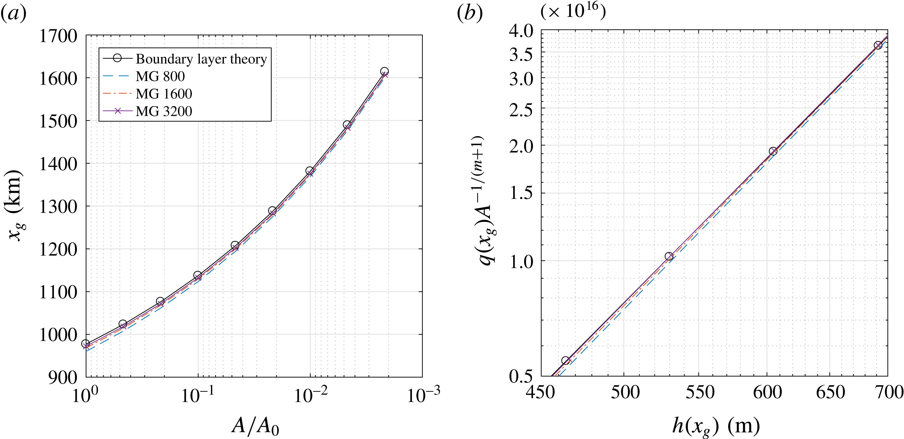
The experiments are similar in set-up to figures 3 and 4 in Pattyn et al. (Reference Pattyn, Schoof, Perichon, Hindmarsh, Bueler, de Fleurian, Durand, Gagliardini, Gladstone and Goldberg2012). The moving grid implementation used here appears to be in good agreement with the boundary layer flux formula. According to Schoof (Reference Schoof2007a ), grounding line flux depends on grounding line ice thickness through a power law, of which the exponent is given by the slope in figure 14(b). The numerical results show a good approximation of the correct slope. Hence, both the grounding line advance and the power law behaviour of the flux are well represented by our implementation.
Grounding line advance throughout the multiple equilibria regime. The moving grid (MG) implementation is again compared against boundary layer theory, for 800, 1600 and 3200 grid points.
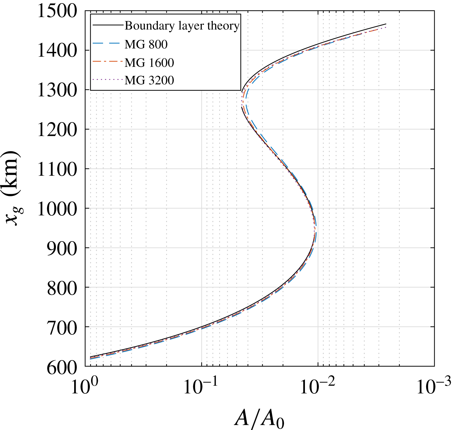
For a final comparison we repeat the computation of the multiple equilibria regime in figure 3 for several grid sizes, see figure 15. The grounding line advance is again compared to boundary layer theory, with a bedrock profile that is now given by (3.1). The grounding line computed using our moving grid implementation is used as initial guess for the Newton iteration solving (C 1). The results show that the computed grounding line advance is again in good agreement with boundary layer theory, with progressively better approximations for increasing grid sizes. The order of this convergence is explored in appendix D. We conclude that the resolution chosen in this paper (1600 grid points) is more than adequate to capture the correct steady state grounding line migration and multiple equilibria regime.
Appendix D. Numerical accuracy of bifurcation points
The results of a convergence experiment are shown in table 4. Let the error in the approximated bifurcation point
 $A_{N}$
be proportional to a power of the mesh width:
 $$\begin{eqnarray}\displaystyle & \displaystyle A_{N}=A+\unicode[STIX]{x1D6FC}(\unicode[STIX]{x0394}z)^{\unicode[STIX]{x1D6FD}}, & \displaystyle\end{eqnarray}$$
where
 $A$
denotes the parameter value at the true bifurcation point and
 $\unicode[STIX]{x1D6FC}$
and
 $\unicode[STIX]{x1D6FD}$
are constants. We define a difference between subsequent mesh halvings
 $D_{N}:=A_{N}-A_{N/2}$
and let
 $\unicode[STIX]{x0394}z\approx 1/N$
. Then the ratio between consecutive differences only depends on the power
 $\unicode[STIX]{x1D6FD}$
:
 $$\begin{eqnarray}\displaystyle & \displaystyle R_{N}=\frac{D_{N/2}}{D_{N}}=\frac{A_{N/2}-A_{N/4}}{A_{N}-A_{N/2}}=\frac{(1/2)^{\unicode[STIX]{x1D6FD}}-1}{(1/4)^{\unicode[STIX]{x1D6FD}}-(1/2)^{\unicode[STIX]{x1D6FD}}}. & \displaystyle\end{eqnarray}$$
From table 4 we suspect
 $R_{N}\rightarrow 2$
as
 $N$
becomes large, corresponding to
 $\unicode[STIX]{x1D6FD}=1$
. The scheme must therefore be of first order accuracy, which is likely due to the first-order upwind discretisation in the continuity equation (A 16). Unfortunately, the upwind discretisation of the ice flux is essential to the stability of the scheme. Hence, it might be worthwhile to consider a higher-order upwind scheme in (A 16).
Convergence of the first bifurcation (point c in figure 3).
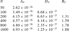
Appendix E. Variability due to noise in buttressing
Temporal variability in buttressing can be interpreted as parameterising a collection of geometric effects, e.g. the occurrence of pinning points and embayments, the creation of ice rumples and the opening of cracks and crevasses. Buttressing has been neglected in our stochastic analyses thus far, as the effect is absent in one horizontal dimension (Gudmundsson Reference Gudmundsson2012). It is possible, however, to introduce a stochastic buttressing coefficient as a parameterisation of an essentially three-dimensional geometric effect.
The influence of buttressing enters through a simple adaptation
 $\unicode[STIX]{x1D703}$
of the grounding line stress (Schoof Reference Schoof2007a
). We let
 $\unicode[STIX]{x1D703}=\bar{\unicode[STIX]{x1D703}}+\unicode[STIX]{x1D702}_{bt}\unicode[STIX]{x1D701}(t)$
, with mean
 $\bar{\unicode[STIX]{x1D703}}$
and standard deviation
 $\unicode[STIX]{x1D702}_{bt}$
. This leads to a multiplicative noise term in the boundary condition (2.4):
 $$\begin{eqnarray}\displaystyle & \displaystyle 2A^{-1/n}\left|\frac{\unicode[STIX]{x2202}u}{\unicode[STIX]{x2202}x}\right|^{1/n-1}\frac{\unicode[STIX]{x2202}u}{\unicode[STIX]{x2202}x}=\frac{\unicode[STIX]{x1D703}}{2}\left(1-\frac{\unicode[STIX]{x1D70C}_{i}}{\unicode[STIX]{x1D70C}_{w}}\right)\unicode[STIX]{x1D70C}_{i}gh\quad \text{at}~x=x_{g}, & \displaystyle\end{eqnarray}$$
where
 $\unicode[STIX]{x1D703}=0$
(
 $\unicode[STIX]{x1D703}=1$
) corresponds to a fully (un)buttressed ice sheet. A linearisation of (E 1) gives a problem with additive noise that we can solve using the elimination approach in § 4.1:
 $$\begin{eqnarray}\displaystyle & \displaystyle 2A^{-1/n}\left|\frac{\unicode[STIX]{x2202}u}{\unicode[STIX]{x2202}x}\right|^{1/n-1}\frac{\unicode[STIX]{x2202}u}{\unicode[STIX]{x2202}x}=\frac{1}{2}\left(1-\frac{\unicode[STIX]{x1D70C}_{i}}{\unicode[STIX]{x1D70C}_{w}}\right)\unicode[STIX]{x1D70C}_{i}g(\bar{\unicode[STIX]{x1D703}}h+\bar{h}\unicode[STIX]{x1D702}_{bt}\unicode[STIX]{x1D701}(t)), & \displaystyle\end{eqnarray}$$
where
 $\bar{h}$
is the equilibrium thickness. Note that we locally introduce a stochastic term that is proportional to the steady grounding line thickness. This leads to an inhomogeneous noise distribution over the ice sheet, similar to the distribution of sea level variability, but now with a significantly larger amplitude.
Standard deviation
 $\unicode[STIX]{x1D70E}_{x_{g}}$
(in m) for five different noise sources at three distinct parameter values, and with a gravitational sea level effect GSLE (cf. the red curves in figures 10–11). The variability due to noise in accumulation (
 $\unicode[STIX]{x1D70E}_{x_{g}}^{ac}$
) and noise in sea level height (
 $\unicode[STIX]{x1D70E}_{x_{g}}^{sl}$
), is compared against variability due to noise in the buttressing coefficient
 $\unicode[STIX]{x1D70E}_{x_{g}}^{bt}$
, with several choices for the standard deviation
 $\unicode[STIX]{x1D702}_{bt}=0.01,0.02,0.04$
.

In table 5 the grounding line standard deviations
 $\unicode[STIX]{x1D70E}_{x_{g}}$
are compared for different noise sources at distinct parameter values
 $A/A_{0}$
, using variable (GSLE) sea level boundary conditions. The standard deviations for accumulation and sea level noise are again
 $\unicode[STIX]{x1D702}_{ac}=\bar{a}/10~\text{my}^{-1}$
and
 $\unicode[STIX]{x1D702}_{sl}=1~\text{m}$
, as in the previous experiments. Since variability in buttressing is not well constrained by observations (Fürst et al.
Reference Fürst, Durand, Gillet-Chaulet, Tavard, Rankl, Braun and Gagliardini2016), we use several choices for the standard deviation
 $\unicode[STIX]{x1D702}_{bt}=0.01,0.02,0.04$
, i.e. fractions of the stress regime from fully buttressed to fully unbuttressed ice sheets. The mean buttressing is taken at
 $\bar{\unicode[STIX]{x1D703}}=1$
, in order to maintain the same dynamical regime that is used in the other noise studies.
The results in table 5 indicate the relative importance of the different noise sources we apply. We find that a variability of only 2 % of the full range of stress conditions induces a noise response of the same order as 10 % variability in accumulation rate. The effect of uncertainty in the buttressing coefficient can therefore not be neglected. More precise measures of temporal buttressing variability are necessary to make a more thorough comparison.


 Open access

