Implications
There is demand for tools to estimate (co)variance matrices with a large number of traits. Different methods to produce large (co)variance matrices were examined using eventing data Great Britain. Two methods that combined sub-matrices from bivariate analyses, as well as an alternative, which performed a 12-trait multivariate analysis using data augmentation and imputation, were found to be appropriate.
Depending on the trait, heritability estimates were 7.2% to 17.1% for dressage, 8.9% to 22.6% for show jumping and 1.3% to 3.9% for cross-country, indicating that genetic progress can be made by selection in the population. Genetic correlations between grades for dressage and show jumping were positive, high and significant, ranging from 0.59 to 0.99, indicating that selection for one grade within these disciplines also selects for other grades.
Introduction
Eventing is the equestrian sport in which the horse and rider compete in each of the three individual competition disciplines – show jumping, dressage and cross-country. Internationally, genetic evaluations for performance in sport horses tend to focus on the individual disciplines of show jumping and dressage, for which many studbooks produce annual breeding value estimates. Genetic evaluations for eventing competition are rare. Langlois (Reference Langlois1980) and most recently Ricard and Chanu (Reference Ricard and Chanu2001) performed evaluations in the French population, the latter using earnings and ranks of the overall competition, and Kearsley et al. (Reference Kearsley, Woolliams, Coffey and Brotherstone2008) performed an evaluation in the horse population of Great Britain (GB), using penalty points, and analysing individual disciplines and an overall trait. The heritability of overall competition in the French population was 0.11/0.17 (annual results; natural log of earnings per number of starts and per number of places, respectively) and 0.07 (rank in each event; Ricard and Chanu, Reference Ricard and Chanu2001). The heritability in the GB population was 0.09 to 0.11 for dressage, 0.08 to 0.23 for show jumping, 0.02 to 0.03 for cross-country and 0.05 for overall competition, using the performance measure of penalty points in a single competition (Kearsley et al., Reference Kearsley, Woolliams, Coffey and Brotherstone2008). These estimates for the show jumping and dressage phases were similar to those derived from evaluations of the individual disciplines.
In GB eventing competition data, there are 12 traits for the combinations of discipline (3) and grade (4; which are, in order of increasing ability, pre-novice, novice, intermediate and advanced). The overall performance in a competition is based on a sum of the scores for the individual disciplines. Ideally, genetic evaluations would be based on a 12-trait model. To enable this, genetic parameters for each of the discipline-grades and correlations between them would need to be estimated. Separate breeding values for each of the 12 competition-grades could then be predicted for each horse. These would be available for all traits, or could be combined into an aggregate index, for example, for each discipline, or for the competition overall. The production of 12 traits, or an index based on these, is of interest as it allows flexibility depending on the breeding goals. For example, breeders may have a particular interest in breeding for a specific level of competition, that is, advanced for the professional rider, or novice for the amateur rider, or the interest may be in producing a horse for competing in one or more of the disciplines.
Genetic evaluations for sport horses typically estimate variance components using residual maximum likelihood (REML), and then predict breeding values using best linear unbiased prediction (BLUP). Most BLUP programs require estimated (co)variance matrices that are positive definite. When the whole matrix is being estimated directly, this frequently results in non-positive definite matrices (negative eigenvalues), and the probability of this increases as the number of traits increases (Hill and Thompson, Reference Hill and Thompson1978). This can be avoided by imposing constraints to keep the matrix positive definite. However, to cope with the computational demands of estimating (co)variance matrices for a large number of traits, often (co)variance matrices are calculated for subsets of the traits, and the estimates are then combined. Again, this frequently results in non-positive definite matrices, and particular methods are required to combine the sub-matrices and produce a positive definite full matrix. Such methods include Mantysaari (Reference Mantysaari2004), which uses a random regression model modified to use a rank-deficient sire (co)variance matrix, Wall et al. (Reference Wall, White, Coffey and Brotherstone2005), which introduced a method based on the Cholesky decomposition, minimising the Frobenius distance (Higham, Reference Higham2002; Sorensen et al., Reference Sorensen, Pong-Wong, Windig and Woolliams2002), among others (Knol and Ten Berge, Reference Knol and Ten Berge1989). A disadvantage of this approach is that combining sub-matrices to form a full (co)variance matrix does not make best use of the available information. Alternatives to REML include Bayesian methods, such as Markov Chain Monte Carlo (MCMC) simulation, which has been used in horse populations (Stock et al., Reference Stock, Hoeschele and Distl2007). A comparison of Bayesian methods and REML is discussed in detail in Misztal (Reference Misztal2008). A feature of MCMC is that it is suitable for multivariate analysis, but may be slow to compute (Misztal, Reference Misztal2008).
This study was driven by the need to develop comprehensive genetic evaluations of horses competing in eventing competitions in GB using the information from all 12 traits in a multivariate fashion. However, the problems encountered in obtaining a positive definite 12 × 12 (co)variance matrix prompted the study to include a comparison of different methodologies.
Material and methods
Data
Competition results, from 1999 to early 2008, were obtained from British Eventing, the body regulating the sport in GB. Results from GB competitors competing in national and international competitions were included. The performance traits used were the penalty point scores for each of the three individual disciplines. Penalty points were converted to normal scores within the competition class, using the method of Kearsley et al. (Reference Kearsley, Woolliams, Coffey and Brotherstone2008), adapted from Royston (Reference Royston1982). The better performing horses were awarded fewer penalty points, and thus a negative Normal score represented a better performance than a positive score. The competition class grouped competitors competing against each other at the same event and covers the standard of the competition, date, location and related temporary environmental factors such as weather. The transformation of penalty points to Normal scores achieved a distribution closer to the Normal, with a zero mean score for each competition class. Horses less than 4 years old were excluded, and horses 20 years or older were grouped into a single age group.
The ability-grade combinations were as follows: dressage pre-novice (DP), dressage novice (DN), dressage intermediate (DI), dressage advanced (DA), show jumping pre-novice (SJP), show jumping novice (SJN), show jumping intermediate (SJI), show jumping advanced (SJA), cross-country pre-novice (XCP), cross-country novice (XCN), cross-country intermediate (XCI) and cross-country advanced (XCA). In the following discussion, those 12 combinations were the 12 traits.
The dressage phase is always performed first, followed by either show jumping or cross-country, depending on the nature of the event. Therefore, the dressage data represented the full number of competition records; subsequent exclusions during the latter phases resulted in slightly less records for them. Records where penalty points did not follow this pattern of performance-related exclusion were removed.
Horses and riders often appear in multiple grades in the data set as a whole. Conversely, some horses may not have competed in all (i.e. the latter) phases of competition because of exclusions, or within every grade; however, because of genetic connections between animals (in this case limited to connections within half-sib groups) and genetic associations between grades and disciplines, breeding values can be predicted for all horses at all grades and disciplines. The rider was considered an important source of variation (Kearsley et al., Reference Kearsley, Woolliams, Coffey and Brotherstone2008) and is estimable because riders are associated with more than one horse (mean number of horses per rider = 2.8), and horses are also commonly associated with more than one rider (mean number of riders per horse = 1.7). Riders have been recorded consistently since 1999; data before this time where rider was intermittently recorded were excluded. The sire of competing horses was available from British Eventing, and was generally well recorded. Sires were recorded by name, however, with no other unique identifiers. Data were cleaned manually, conservatively grouping sire names where they were considered to be the same animal. Variance components were estimated using a data set reduced in size to include sires with either (i) 30 or more individual progeny competing in either pre-novice or novice grades or (ii) any progeny in intermediate or advanced grades.
Models
The basic model was a sire model with mixed linear effects, fitted within each discipline-grade:

The fixed effects were gender of the horse (‘gender’: stallion, geldings and mares), the age of the horse at the time of competition fitted as linear and quadratic covariates and competition class (‘class’). Random effects were the additive genetic effect of the sire (‘sire’), the rider (‘rider’), the permanent environment of the horse (‘horse’) and the residual error (e). The random effects of the sire, rider, horse and residual error were assumed to be normally distributed with (co)variance matrices Σ sire⊗I, Σ rider⊗I, Σ horse⊗I and Σ e⊗I.
Owing to computational constraints, it was impossible to perform a standard 12-trait multivariate analysis for the full model, and thus three alternative methods were used to estimate the 12 × 12 (co)variance matrices. The relationship between traits was assumed to be unstructured, that is, there were no specified correlations between grades.
Method 1
A method called data augmentation was used to perform a 12-trait multivariate analysis. This data augmentation is based on work by Thompson (Reference Thompson1994) and Clayton and Rasbash (Reference Clayton and Rasbash1999) where computational requirements are reduced, using data with hierarchically nested random effects, by repeatedly fitting sub-models in an overlapping series, with each sub-model being fitted in turn to data adjusted for effects not in the current sub-model. In an iteration of the full model, an internal iteration of each sub-model is performed. This greatly reduces the computational requirements. Fixed and random effects are updated as they are re-estimated. A simplified form of Gibbs sampling is used to add noise to the updated estimates at each step, thus preventing bias in the estimated effects. For random effects, the noise added to each solution is taken as a sample from a normal distribution with a variance equal to the prediction error variance of that solution; for fixed effects, the noise is sampled from a normal distribution with variance equal to the square of the standard error. The calculations were carried out in a development version of ASReml 3 (Gilmour et al., Reference Gilmour, Gogel, Cullis and Thompson2009).
For example, if the two sub-models are: (1) y − Zu = Xβ + e and (2) y − Xβ = Zu + e, where y is a vector of phenotypic observations, u and β are vectors of random and fixed effects respectively, e is a vector of residual errors, Z and X are design matrices allocating observations to random and fixed effects, the process is as follows:
-
(i) For model 1, assume u is 0, estimate and add noise to β.
-
(ii) For model 2, augment the data by subtracting Xβ using an imputed value of β from (i), estimate u and variances and add noise to u.
-
(iii) For model 1, augment the data y by subtracting Zu using an imputed value of u from estimate of u from (ii), estimate and add noise to β.
-
(iv) Repeat (ii) and (iii), for total number of iterations.
-
(v) Exclude burn-in iterations, and calculate averages of estimates.
In this analysis, the full model was split into four sub-models. These were: (1) the fixed effect of class within discipline and grade, (2) the random effect of sire within discipline and grade, (3) the random effect of rider within discipline and grade and (4) the random effect of horse within discipline and grade. The fixed effects of gender within discipline and grade and age (linear) and age (quadratic) within discipline and grade were included in all sub-models. A burn-in period of 60 iterations was allowed, and 500 iterations were executed. Residual error covariances were fixed at zero because, as a simplification, it was assumed that there was no covariance between discipline-grades for the remaining un-explained variance. (Co)variance matrices for each random effect were estimated as the average overall iterations excluding the burn-in period, making a total of 440 iterations.
The 12-trait multivariate model (before division into sub-models) was

where y is a matrix of responses and dg is the factor indicating discipline-grade. The fixed effects were gender of the horse (‘gender’), age of horse at the time of competition (polynomial, linear and quadratic) and competition class (‘class’). Random effects were the additive genetic effect of the sire (‘sire’), the rider (‘rider’), the permanent environment of the horse (‘horse’) and the residual error (e). The random effects sire, rider, horse and residual error were assumed to be normally distributed with (co)variance matrices Σ sire⊗I, Σ rider⊗I, Σ horse⊗I and Σ e⊗I. The estimated matrices were constrained to be positive definite by performing an expectation-maximisation update if the average information REML update generated a non-positive definite matrix.
The analysis gives solutions plus their standard errors for all fixed and random effects. Unfortunately, as yet no standard errors are available for estimates of variance components; therefore, estimates of standard errors from the bivariate analyses were used (see section ‘Methods 2a/2b’ below). The standard errors from the various models are unlikely to differ much, and we might expect the standard errors from a 12-trait analysis to be lower than the standard errors obtained if only 2 of the 12 traits were included in the analysis. For this model, standard errors of correlations between traits are approximate.
Methods 2a/2b
A series (66) of bivariate analyses, for every possible pair of discipline-grade traits, was run using ASReml. Two distinct methods were then used to combine the series of 2 × 2 sub-matrices from each strata (sire, horse, rider) into the 12 × 12 covariance matrices.
Method 2a: For each of the 66 bivariate analyses, three pairs of observations were sampled from a multivariate Normal distribution defined by the 2 × 2 covariance matrix. These were analysed in a 12-trait multivariate analysis using ASReml, where the only fixed effect in the model was a separate mean for each of the 66 bivariate analyses. At least three samples were required to ensure that the resulting (co)variance matrix matched the (co)variance matrix from the bivariate analysis. This is an extension of Wall et al. (Reference Wall, White, Coffey and Brotherstone2005), designed to ensure that a mean could be fitted in the final model.
Method 2b: The average (co)variance values for the 66 bivariates were calculated as simple means. To convert these average (co)variance matrices into positive definite matrices, they were decomposed to give the eigenvalues and eigenvectors. Negative eigenvalues were changed to 1 × 10⁻¹⁰ and the matrices were re-composed. This method is a simplification of more complex methods that minimise the Frobenius distance between the original estimate and the final positive definite estimate (Higham, Reference Higham2002; Sorensen et al., Reference Sorensen, Pong-Wong, Windig and Woolliams2002), that is, equivalent to computing the positive definite matrix that is best fitting by least squares (Knol and Ten Berge, Reference Knol and Ten Berge1989). Standard errors of correlations were not accounted for in the process.
Thus, three methods were used to produce the positive definite 12 × 12 (co)variance matrices, suitable for BLUP estimation of breeding values. To estimate the effect of fixed effects for Methods 2a/2b, the results from the 66 bivariates were averaged.
Calculation of functions of variance components
Heritabilities (h
2), repeatabilities (r
2) and fractions of variance due to permanent environment (c
2) and rider (w
2) were calculated as functions of the various components using the phenotypic variance defined as  . The functions were calculated as
 and
 where is the total variance,
 is the sire variance,
 is the residual horse variance,
 is the rider variance and
 is the residual variance.
Results
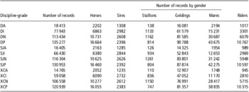
Table 1 summarises the data set, giving the number of records, horses, sires, number of records by horse gender and number of riders for each discipline-grade in the data set.
Number of records, horses, sires, number of records by horse gender and number of riders for each discipline-grade in the data set (the total number of horses, sires and riders was 19829, 3017 and 11841, respectively)

DA = dressage advanced; DI = dressage intermediate; DN = dressage novice; DP = dressage pre-novice; SJA = show jumping advanced; SJI = show jumping intermediate; SJN = show jumping novice; SJP = show jumping pre-novice; XCA = cross-country advanced; XCI = cross-country intermediate; XCN = cross-country novice; XCP = cross-country pre-novice.
Comparison of models
The computing resources required by the data augmentation method were extremely small compared with the bivariate methods. Overall, fitting the data augmentation model took ∼7 h, compared with ∼4 h for each of the 66 bivariates (i.e. 264 h in total). All runs were performed on a computer with a 2.4 GHz clock speed. The bivariate analyses were each allowed up to 4 GB of memory and the data augmentation method up to 8 GB. The differences in the (co)variances and solutions produced by the three methods were used to compare models.
Phenotypic variance
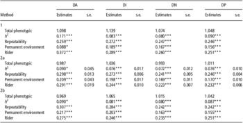
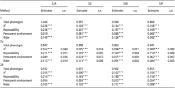
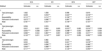
As the trait was a normal score (mean 0, standard deviation 1), the phenotypic variance is expected to be ⩽1, depending on class sizes. Estimates of the total phenotypic variance for the three methods are shown in Tables 2 to 4. Estimates from all methods were close to the anticipated value of 1. Estimates from the data augmentation method had a greater range over the disciplines, compared with the bivariate methods, and tended to be higher within the more advanced grades.
Functions of variance components for dressage as estimated by the three methods

DA = dressage advanced; DI = dressage intermediate; DN = dressage novice; DP = dressage pre-novice.
*P < 0.05, **P < 0.01, ***P < 0.001.
Functions of variance components for show jumping as estimated by the three methods

SJA = show jumping advanced; SJI = show jumping intermediate; SJN = show jumping novice; SJP = show jumping pre-novice.
*P < 0.05, **P < 0.01, ***P < 0.001.
Functions of variance components for cross-country as estimated by the three methods

XCA = cross-country advanced; XCI = cross-country intermediate; XCN = cross-country novice; XCP = cross-country pre-novice.
*P < 0.05, **P < 0.01, ***P < 0.001.
Heritabilities
Heritability estimates for the 12 traits, as estimated by the different methods, are given in Tables 2 to 4 for the individual disciplines.
Irrespective of the method of analysis, heritabilities were significantly >0 for all traits excluding the higher grades in cross-county. Show jumping showed the greatest heritability, followed by dressage and then cross-country.
From Method 1, the advanced grade of all disciplines had the highest heritability (Tables 2 to 4). This was particularly true for dressage (17.1%) and show jumping (22.6%). The remaining grades of dressage were very consistent (8.0% to 9.0%). For show jumping, pre-novice grade had the lowest heritability (10.6%). Note that the higher heritability estimates were associated with both higher phenotypic and higher genetic variance.
Comparing Methods 2a and 2b, the differences were slight, with the greatest absolute difference in heritability estimates being 1.5%, and because the standard error of the estimate was 0.9% this was likely to have been a chance occurrence. The standard errors were taken as averages over the bivariate analyses. Given this small difference, only Method 2a will be described more fully.
The pattern of magnitudes of heritability across disciplines and grades was similar to Method 1, with show jumping having the highest heritability (8.9% to 16.2%), followed by dressage (7.2% to 9.0%) and then cross-country (0.3% to 1.4%) and estimates of heritability tending to be greatest in advanced grade.
Repeatabilities
Repeatability estimates, which are the proportion of phenotypic variance explained by the horse genetics and the horse's permanent environment combined, represent the upper limit to the heritability. These are also given in Tables 2 to 4. Methods 2a and 2b were in good agreement. Estimates from Method 2a were highest for dressage, 24.1% to 29.8%, followed by show jumping, 15.8% to 21.0%, with cross-country being the lowest again (8.5% to 9.8%).
Although the pattern was similar for Method 1, there were differences: for dressage at advanced grade, the estimate was lower compared with the bivariates; for show jumping at advanced and intermediate grades, the estimates were higher; and for all grades of cross-country, estimates were slightly higher. However, there is no evidence to suggest that these differences are statistically significant.
Horse's permanent environmental variance
The proportion of phenotypic variance explained by the permanent environment of the horse is given in Tables 2 to 4. The permanent environmental variance is the variance due to environmental effects that have consistently influenced the horse's performance, such as long-term training, stabling, any early-life influences and also, in this analysis, the maternal effects that cannot be identified, as dams were unknown. Estimates were again very similar between Methods 2a/2b. For Method 2a, the permanent environment accounted for 16.9% to 20.9% of phenotypic variance in dressage compared with 4.9% to 7.5% in show jumping and 6.6% to 8.7% in cross-country. The large estimate for the influence of permanent environment on dressage performance compared with show jumping explains why the repeatability is estimated to be greater for dressage, yet its heritability appeared smaller.
For Method 1, estimates were consistent with Methods 2a/2b, with the exception of advanced grades in dressage and show jumping, which were noticeably smaller. For dressage, estimates ranged from 8.8% to 18.9% and for show jumping from 16.9% to 24.6%.
Rider variances as a proportion of total variance
The estimates of variance due to the rider were very similar when estimated by Methods 2a and 2b. The maximum absolute difference in the estimates was 2.7% of total phenotypic variance (standard error on rider variance was 0.6%). The proportion of variance due to the rider, as estimated by Method 2a, was 22.3% to 29.1% for dressage, 8.4% to 11.3% for show jumping and 9.2% to 12.0% for cross-country. Estimates by Method 1 tended to be greater in magnitude than Method 2a/2b estimates.
Genetic correlations
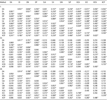
Genetic correlations are presented in Table 5. Correlations within grades were all significant. For dressage, these ranged from 0.783 to 0.946; for show jumping, from 0.803 to 0.954; and for cross-country, from 0.358 to 0.698. There was a clear pattern that correlations between sequential grades were higher than those between more distant grades. Results from Methods 2a and 2b were very similar. For both methods, genetic correlations between the grades were significantly different from zero for dressage and show jumping, positive and high (for dressage 0.59 to 0.99, for show jumping 0.74 to 0.99). For cross-country, there is a need for greater caution as genetic correlations between the grades were only significantly different from zero between novice and pre-novice, with an estimate of 0.75. This provides evidence that for dressage and show jumping, and at least within lower grades of cross-country, within the discipline, the same loci (or loci in linkage disequilibrium) are predominantly responsible for performance at the different grades.
Horse (below diagonal) and genetic (above diagonal) correlation matrices for the 12 traits, as estimated by the three different methods

DA = dressage advanced; DI = dressage intermediate; DN = dressage novice; DP = dressage pre-novice; SJA = show jumping advanced; SJI = show jumping intermediate; SJN = show jumping novice; SJP = show jumping pre-novice; XCA = cross-country advanced; XCI = cross-country intermediate; XCN = cross-country novice; XCP = cross-country pre-novice.
*Correlation significantly greater than zero (P < 0.05); figures in italics were estimated at the boundary and no standard errors were available.
For Method 1, correlations between disciplines were largely significant. Between show jumping and dressage, significant correlations ranged from 0.011 to 0.385, but estimated correlations between cross-country and other disciplines appeared more heterogeneous in sign ranging from −0.163 to 0.093 for dressage. By contrast, from Methods 2a and 2b between-discipline correlations were largely not significant, but also of varied sign and magnitude. Correlations between the lower grades of dressage and show jumping were statistically significant, positive but low, and a low significant correlation between show jumping and XCP and XCN was found. Estimates for dressage and cross-country were indicative of there being negative correlations of moderate magnitude. For Method 2b, comparing the genetic correlation matrix before and after bending (considering only estimates that were significantly different from zero in the positive definite matrix), the average absolute change was 0.054.
Horse and rider correlations
Correlations for the horse (representing the permanent environment and 3 × the sire genetic component) between grades and within disciplines were all significant and generally high (Table 5). Rider correlations are in Table 6.
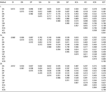
Rider correlation matrices for the 12 traits, as estimated by the three different methods

DI = dressage intermediate; DA = dressage advanced; DN = dressage novice; DP = dressage pre-novice; SJA = show jumping advanced; SJI = show jumping intermediate; SJN = show jumping novice; SJP = show jumping pre-novice; XCA = cross-country advanced; XCI = cross-country intermediate; XCN = cross-country novice; XCP = cross-country pre-novice.
Correlations other than those in italics were significantly greater than zero (P < 0.05); figures in italics were estimated at the boundary and no standard errors were available.
From Model 1, correlations between disciplines were largely significant, although low/moderate. Correlations between show jumping and cross-country were slightly higher than between other disciplines. Rider correlations were all significant. Within-discipline correlations were very high. Between-discipline correlations were moderate/high, although slightly lower between dressage and cross-country compared with the other disciplines.
By Method 2b, horse correlations within disciplines were 0.64 or more for dressage, but showed a greater range of 0.36 to 0.96 for show jumping and 0.10 to 0.80 for cross-country. The correlation structures were clearly banded, with high or moderate correlations observed between adjacent grades, lower correlations between grades once removed and lowest between pre-novice and advanced. Significant correlations between disciplines were positive but low. In general, rider correlations, both within and between disciplines, were significant. Within-discipline correlations were high, and between-discipline correlations were generally moderate.
Comparison of correlation estimates between Method 2a and Method 1
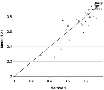
Figure 1 shows a more detailed comparison of methods restricted to estimates that were within discipline and statistically different from 0 (based on s.e.). The genetic correlations, once away from 1, showed more scatter, probably because of their greater sampling error. The horse correlations, comprising both the genetic and permanent environment, were broadly in agreement between the methods, with no evidence of consistent bias. For the rider correlations, again there was no evidence of a consistent bias between methods.
Estimates of correlations within grades for the genetic (black), horse (white) and rider (grey) effects plotted for Method 1 v. 2a. Only correlations where standard errors indicated that values were significantly different from zero are included.

Between-discipline correlations were different (not shown). There was a consistent trend for Method 1 to estimate genetic correlations or horse correlations that were larger than for Method 2a (with the comparison restricted to those that were judged to be statistically significant). The same was true for rider correlations, with the exception of correlations including some of the more advanced grades, where estimates by Method 2a were often higher than Method 1.
Fixed effects of gender and age
For the effects of gender, for all models, there were generally significant gender effects for dressage, but not for the other disciplines. For dressage, stallions and geldings performed significantly better than mares in most grades. For show jumping, estimates were in general not significant, but stallions performed better than mares and mares performed better than geldings. For cross-country, by Method 1, geldings performed better than mares, and mares better than stallions. For the Methods 2a and 2b, there were no discernable differences for cross-country.
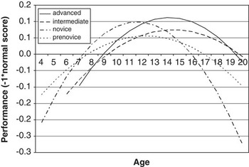
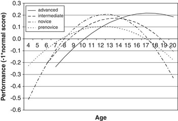
For all models and all traits, there was a significant quadratic association between performance and age, indicating a curvilinear increase in performance with age. Figures 2 to 4 illustrate the change in performance with age, using example results from the bivariate analyses. As might be predicted, performance in the more advanced grades peaked at a later age. For all disciplines, similar patterns were observed, although between disciplines peak performance between grades varied and was least pronounced in show jumping.
Performance with age for each grade of dressage.

Performance with age for each grade of show jumping.

Performance with age for each grade of cross-country.

Discussion
There is a demand for tools to estimate (co)variance matrices for a large number of traits in an acceptable time frame. The current test day model used by the dairy cattle industry in the United Kingdom requires a 27 × 27 (co)variance matrix, and other industries may desire even larger matrices. For example, a BLUP with 100 traits would be ideal for the silvicultural objectives of Skogforsk (the Forestry Research Institute of Sweden; B. Andersson, personal communication, December 2010). A rapid analysis would enable easy re-estimation of (co)variance matrices, rather than the current situation where in many genetic evaluation systems, due to computing overheads, the (co)variance components are not re-estimated regularly and BLUP estimated breeding values (EBVs) are being produced based on variance components compiled using ad hoc methods from old data. Therefore, any method offering an advance in such methodology would have important applications.
We compared three methods of producing large (co)variance matrices for genetic evaluations, using a data set of results from eventing competitions in the United Kingdom. Two methods that combined smaller sub-matrices from bivariate analyses were investigated: (i) Method 2a, a novel method based on Wall et al. (Reference Wall, White, Coffey and Brotherstone2005) that generates samples of each bivariate distribution to perform a multivariate analysis and obtain a positive definite 12 × 12 (co)variance matrix and (ii) Method 2b, spectral decomposition of the matrix of mean results replacing negative eigenvalues with positive values to obtain a positive definite (co)variance matrix. The latter is likely to be relatively well applied in practice. The two ‘bivariate’ methods, differing only in the way that the bivariate matrices were combined, gave, in this case, very similar results for functions of variance components. Method 1 was the novel data augmentation function in ASReml. The multivariate nature of Method 1 will result in greater accuracy (with the increase in accuracy determined by the absolute differences between the residual and genetic correlations between traits).
(Co)variance estimates and functions of variance components produced by the three methods were in general similar. Correlation estimates were more often significant for Method 1, which may be partially due to the fact that standard errors for these values were approximate values.
As the trait was a normal score (mean 0, standard deviation 1), the variance of each trait would be expected to be ⩽1, depending on class sizes. In the data augmentation analysis, the increase in phenotypic variance with grade within a discipline could be explained by the fact that Method 1 was a 12-trait analysis, with information on performance at all grades included and thus the analysis at least partly accounts for selection between grades, as well as producing more accurate variance component estimates. It would also be feasible to obtain phenotypic variances >1 when analysing heritable traits with substantial inbreeding with a pedigree of many generations in depth. However, in this analysis, it was only possible to use a sire model that makes no allowances for inbreeding.
No formal comparison of the fits of the models could be performed. The three methods produced largely consistent results. Methods 2a and 2b are suitable for implementation and will produce large, positive definite (co)variance matrices, but require large computing resources. Method 1 produced results that were generally consistent with Methods 2a and 2b. Method 1 enables the production of large (co)variance matrices in a computationally efficient way, and harvests the full benefits of a multivariate analysis. Differences in variance component estimates between Methods 1 and 2a/2b may be due to the increased accuracy of Method 1, a result of the multivariate nature of the analysis.
The heritability estimates for the dressage phase of the competition are comparable with estimates for the individual competition discipline in GB, which were 0.15 (s.e. 0.018) when breed is not accounted for (Stewart et al., Reference Stewart, Woolliams and Brotherstone2010), and also with international estimates. For example, heritabilities ranging from 0.10 to 0.20 have been estimated in various breeds (see Huizinga and Van Der Meij, Reference Huizinga and Van Der Meij1989; Ricard et al., Reference Ricard, Bruns and Cunningham2000; Ducro et al., Reference Ducro, Koenen, van Tartwijk and van Arendonk2007; Janssens, Reference Janssens2008; Olsson et al., Reference Olsson, Näsholm, Strandberg and Philipsson2008). Similarly, heritability estimates for show jumping are comparable to international estimates for competition data, ranging from 0.10 (Hanoverian, Trakehner, Oldenburg; Janssens, Reference Janssens2008) through 0.20 in Dutch Warmbloods (Huizinga and Van Der Meij, Reference Huizinga and Van Der Meij1989) to 0.27 in the Swedish Warmblood (Olsson, Reference Olsson, Näsholm, Strandberg and Philipsson2008).
The genetic variation detected in the analysis for cross-country was low and to some extent it may be masked by greater environmental variance. Improved pedigree data may help to elucidate the genetic variation further. However, our results indicate that in a selection programme, the greatest genetic gain can be achieved in show jumping, followed by dressage, and that little gain will be made in cross-country. Therefore, a breeding programme designed to select for eventing competition performance in GB will be best suited to select for the show jumping or dressage phases of the competition. Even if this were considered as a phenotypic selection rather than a selection for breeding, performance at lower grades was a poorer predictor of performance at high grade for cross-country than for show jumping or dressage. At present in the United Kingdom, the situation in practice is directly contrary to this, as breeders of eventing horses tend to consider cross-country performance as the primary selection aim (J. Rogers, personal communication, May 2010). This traditional practice is derived from the origins of the discipline that originated in the Military and was dominated by cross-country. Greater weighting was placed on cross-country, with requirements for dressage and show jumping lower. The dressage phase was aimed at increasing the control the rider has over the horse, and the show jumping phase was used to test the recovery of the horse after a cross-country competition. More recently, because of international influences, the regulation of the discipline has changed. A lower weight has been given to cross-country, which is judged to be too dangerous and less and less conforming to animal welfare regulations. This has changed the type of horses needed to compete in this discipline.
Within the disciplines of dressage and show jumping, correlations between the grades were high, indicating that the same loci (or loci in linkage disequilibrium) are responsible for performance at the different grades, and therefore selection for performance in one grade also selects for performance in another grade. Analogous correlations between the grades for cross-country were estimated by Method 1 as significantly different from zero but more moderate; results by Methods 2a/2b were harder to estimate partly due to a lack of genetic variance detected, particularly in the higher grades.
Overall, the results from the data augmentation method indicate that selection for performance in dressage will improve performance in show jumping and that performance in show jumping will improve performance in cross-country. There was an indication that selection for dressage merit would reduce the merit for cross-country. Higher correlations between the lower grades may be due to general traits that jointly affect performance in both, that is, an amateur horse that is athletic and with good temperament should have good ability, at lower levels of competition, in all disciplines. However, at the highest grade of competition these effects are less apparent, where more specific traits, such as the gaits and jumping, have more influence on performance.
Variance components due to the horse and rider were considered separate random effects. This was possible because of the fact that one rider often rode multiple horses, and that many horses were ridden by multiple riders. If the latter were not true, different treatments of the rider effect within the model could be considered. For instance, a hierarchical model (of horse within rider) could be used. Alternatively, rider could have been included as a fixed effect.
Gender effects for show jumping and particularly dressage found indication of an advantage for stallions. Given that stallions are a selection of the male population retained for breeding, this is understandable. However, gender effects were often not significant. It was surprising that no gender effect was detected for cross-country, as there is clear evidence of an advantage for males as evidenced for racing (Entin, Reference Entin2008).
The analysis was restricted to a sire model, and thus genetic connections were limited (restricted to within half-sib groups). Although this was sufficient to proceed with the analysis, the precision of the estimates of variance components and EBVs will have been reduced, with this reduction reflected in the standard errors. Assortative mating was not accounted for, possibly inflating the sire variance component, and overestimating EBVs for superior sires (and underestimating for inferior sires). Selection and inbreeding were also not accounted for. In horse populations, the assumption of random mating rarely holds. Selection has been practised over time and non-random mating occurs, in that superior horses tend to be mated as do inferior horses, and there may be specialised breeding for the different disciplines. Another potential problem is the selection of horses present in the data. The consequence of this will be to reduce heritability estimates.
The breeding objective for the British sport horse is to cater for both professional elite levels of competition and riders, as well as amateur riders. Traits such as athleticism, soundness, rideability and conformation suitable for competing in a range of disciplines, including dressage, show jumping and eventing, are required. The data augmentation 12-trait analysis enables all traits to be considered in the analysis, and thus the accuracy of breeding values is maximised. The results for the analysis suggest that there are positive genetic correlations between dressage and show jumping and show jumping and eventing, indicating that selection for one discipline will also enhance performance in another. However, correlations between eventing and dressage were sometimes negative. The British sport horse has made its name in eventing competition, and thus selection for this discipline may reduce performance in dressage.
There is little literature assessing genetic correlations between adult competition disciplines; instead, data tend to be sourced from young horse tests. Internationally, estimates for genetic correlations between dressage and show jumping related traits at young horse tests are generally low and mixed (either positive or negative), although correlations between canter and jumping tend to be higher than correlations between the other gaits and jumping (Thorén Hellsten et al., Reference Thorén Hellsten, Viklund, Koenen, Ricard, Bruns and Philipsson2006). This study adds some evidence to this area, indicating that simultaneous selection for both dressage and show jumping may hinder genetic progress for the disciplines individually.
Twelve breeding values for each of the discipline-grade traits are now available. These can be combined into an index for overall competition performance, with weightings depending on the breeding purpose. In breeding for elite levels of competition, performance at the more advanced grades is important. However, a main aim of sport horse breeding in the United Kingdom is to produce horses for amateur and young riders, which constitute the vast majority of the riding and competing population, and for which traits such as temperament and general ability have most influence. The accuracy of the breeding values at lower and intermediate levels of competition is likely to be higher, as the accuracy of breeding values is dependent on the number of records. At advanced grade, a horse may compete far less than at lower grades (possibly only four times per year), resulting in fewer records and hence lower accuracies for advanced breeding values.
In conclusion, this work investigated three methods of estimating large (co)variance matrices. Two of these methods, based upon bivariate analysis, are computing intensive but reliable and appropriate for implementation at present. The third method (using data augmentation) requires far fewer computing resources, is much quicker to run, and will be valuable in the future for the production of large (co)variance matrices.
Acknowledgements and funding
The authors would like to thank BBSRC, British Equestrian Federation (BEF) and Biosciences KTN for funding and British Eventing for providing data. This work has made use of the resources provided by the Edinburgh Compute and Data Facility (ECDF; http://www.ecdf.ed.ac.uk/). The ECDF is partially supported by the eDIKT initiative (http://www.edikt.org.uk).