1 Introduction
The logarithmic region (log layer) of the boundary layer is a subject of significant interest in the study of wall-bounded turbulent flows. However, the region only exists for relatively large Reynolds numbers when there is a layer sufficiently separated from both the wall and the free stream to not be directly affected by either viscosity
 $\unicode[STIX]{x1D708}$
or the boundary layer depth
 $\unicode[STIX]{x1D6FF}$
(Pope Reference Pope2000). The characteristic scales in the logarithmic region are the shear or friction velocity
 $U_{\unicode[STIX]{x1D70F}}$
and the wall-normal distance
 $z$
(see e.g. Prandtl Reference Prandtl1925; von Kármán Reference von Kármán1931; Townsend Reference Townsend1976). The characteristic Reynolds number in this case is the friction Reynolds number
 $Re_{\unicode[STIX]{x1D70F}}=\unicode[STIX]{x1D6FF}U_{\unicode[STIX]{x1D70F}}/\unicode[STIX]{x1D708}$
.
In the past few decades, there has been the development of new laboratory-scale facilities capable of reaching
 $Re_{\unicode[STIX]{x1D70F}}\sim O(10^{4}{-}10^{5})$
which has allowed for the study of the logarithmic region and scaling behaviour across at least a decade of
 $Re_{\unicode[STIX]{x1D70F}}$
(see e.g. Smits, McKeon & Marusic Reference Smits, McKeon and Marusic2011; Marusic et al.
Reference Marusic, Monty, Hultmark and Smits2013). These facilities include, in decreasing order of
 $Re_{\unicode[STIX]{x1D70F}}$
, the Princeton Superpipe (Zagarola et al.
Reference Zagarola, Smits, Orszag and Yakhot1996), the US Navy’s William B. Morgan Large Cavitation Channel (Etter et al.
Reference Etter, Cutbirth, Ceccio, Dowling and Perlin2005) and the Melbourne wind tunnel (Nickels et al.
Reference Nickels, Marusic, Hafez and Chong2005). While the laboratory-scale facilities can reach velocities comparable to large-scale systems, a key limitation is the restriction of the boundary layer depth to less than
 $\unicode[STIX]{x1D6FF}\sim O$
(1 m). The boundary layer – and as a result the log layer – is orders of magnitude smaller than many natural and engineered systems.
One such system is the atmospheric surface layer (ASL), where the surface layer designation indicates the bottom portion of the planetary boundary layer. The surface layer depth is typically of the order
 $\unicode[STIX]{x1D6FF}=O$
(100 m), and the planetary boundary layer extends to 1 km (Stull Reference Stull1988; Kaimal & Finnigan Reference Kaimal and Finnigan1994). Within the surface layer, Coriolis effects are negligible, and the Reynolds shear profile is approximately constant (Sutton Reference Sutton1953). The behaviour above the ASL poses complications not present for laboratory free-stream conditions, but turbulence within the surface layer is primarily driven by mechanical shear when thermal conditions are neutrally stable. Under neutral conditions, the surface layer exhibits logarithmic behaviour in the mean velocity throughout its depth
 $\unicode[STIX]{x1D6FF}$
(Kaimal & Finnigan Reference Kaimal and Finnigan1994).
The flow qualities in the ASL – shear-driven, constant shear stress, logarithmic mean velocity profile – create the potential for the ASL to be studied as a canonical very-high-
 $Re$
boundary layer with an extensive log layer. However, this characterization only holds when the temperature profile is neutrally stratified. When a significant temperature gradient is present, as is often the case in the diurnal temperature cycle, conditions are either thermally unstable (convective) or stable and turbulence is respectively enhanced or dampened by buoyancy effects (Stull Reference Stull1988). Weather effects pose additional challenges to studying atmospheric turbulence. Time-varying mean wind conditions make it difficult to define turbulent fluctuations and to distinguish the largest turbulent flow scales from weather-related mesoscales.
In an attempt to study turbulent boundary layers at the atmospheric scale, two notable field stations have been established in quasi-smooth wall environments: the Surface Layer Turbulence and Environmental Science Test (SLTEST) site in the salt flats of Utah (Metzger & Klewicki Reference Metzger and Klewicki2001; Metzger, McKeon & Holmes Reference Metzger, McKeon and Holmes2007) and the Qingtu Lake Observation Array (QLOA) on a dry lake bed in western China (Wang & Zheng Reference Wang and Zheng2016). Both facilities use a vertical and a spanwise array of hot-wire and sonic anemometers. By considering only periods of near-neutral stability and through careful treatment of data, studies at these facilities have shown canonical boundary layer profiles in first- and second-order statistics (Hutchins et al. Reference Hutchins, Chauhan, Marusic, Monty and Klewicki2012; Wang & Zheng Reference Wang and Zheng2016). The point measurements have also led to numerous insights, primarily related to large-scale turbulent motions (Guala, Metzger & McKeon Reference Guala, Metzger and McKeon2011; Wang & Zheng Reference Wang and Zheng2016). However, the study of turbulent structures at these facilities is ultimately limited by the spatial resolution determined by the spacing between anemometers.
An attractive option for improving the spatial resolution of field-scale measurements is the use of particle image velocimetry (PIV). This technique has been applied at the SLTEST facility using upwind generated smoke or fog as seeding particles (Hommema & Adrian Reference Hommema and Adrian2003; Morris et al.
Reference Morris, Stolpa, Slaboch and Klewicki2007). For this case the analysis is constrained to the near-wall region and the flow seeding is non-uniform. In a major advancement of field-scale PIV, recent studies at the Eolos field facility in Minnesota have validated the use of snow particles as tracers for super-large-scale PIV (SLPIV) (Hong et al.
Reference Hong, Toloui, Chamorro, Guala, Howard, Riley, Tucker and Sotiropoulos2014; Toloui et al.
Reference Toloui, Riley, Hong, Howard, Chamorro, Guala and Tucker2014). The spatial domain, illuminated by a light sheet, can reach heights above 100 m (Hong et al.
Reference Hong, Dasari, Wu and Liu2017). The SLPIV technique has high spatial resolution relative to field point measurements in two directions. Compared with laboratory-scale PIV, the spatial resolution is coarse when scaled in inner wall units (
 $\unicode[STIX]{x1D708}/U_{\unicode[STIX]{x1D70F}}$
), but is finer when scaled in outer units (
 $\unicode[STIX]{x1D6FF}$
) and provides an unprecedented number of measurement points within the logarithmic region. SLPIV thus allows the opportunity to spatially investigate coherent structures in the very-high-
 $Re$
ASL. In the present work, we report new SLPIV velocity measurements in the logarithmic region of the ASL in a fully rough environment.
With the new measurements, we seek to provide insight into the ongoing research of coherent structures populating turbulent flows. Probably the most controversial and well-studied coherent structure is the hairpin vortex, a horseshoe-shape vortex with legs originating near the wall and a forward-inclined arch. Hairpin vortices were first theorized over 60 years ago by Theodorsen (Reference Theodorsen1952) and received limited support in the intervening years (see e.g. Offen & Kline Reference Offen and Kline1974). Strong experimental support for hairpin vortices came from Head & Bandyopadhyay (Reference Head and Bandyopadhyay1981), who identified hairpin vortices organized in packets. Packets of hairpin vortices have since become an area of extensive research (Adrian Reference Adrian2007). The structure of these vortex packets has been studied in experiments (Adrian, Meinhart & Tomkins Reference Adrian, Meinhart and Tomkins2000b ; Christensen & Adrian Reference Christensen and Adrian2001; Ganapathisubramani, Longmire & Marusic Reference Ganapathisubramani, Longmire and Marusic2003; Tomkins & Adrian Reference Tomkins and Adrian2003; Ganapathisubramani et al. Reference Ganapathisubramani, Hutchins, Hambleton, Longmire and Marusic2005; Wu & Christensen Reference Wu and Christensen2006; Dennis & Nickels Reference Dennis and Nickels2011; Herpin et al. Reference Herpin, Stanislas, Foucaut and Coudert2013) and numerical simulations (Zhou et al. Reference Zhou, Adrian, Balachandar and Kendall1999; Wu & Moin Reference Wu and Moin2009; Lee & Sung Reference Lee and Sung2011). The packets are believed to exist in a hierarchy and evolve through mechanisms including self-induction, lift-up and merging (Adrian Reference Adrian2007). Packet size is believed to increase with wall-normal distance, but the quantification of hairpin packet wall-normal trends is often limited by the small logarithmic layer thickness achieved in laboratory settings.
More generally, ramp-like structures share the same broad characteristics as hairpin packets – namely their forward inclination – without necessarily distinguishing individual vortices. Ramp-like structures have been confirmed statistically by identifying inclined two-point correlations for wall-bounded flows including rough wall boundary layers (Volino, Schultz & Flack Reference Volino, Schultz and Flack2007; Guala et al. Reference Guala, Tomkins, Christensen and Adrian2012; Squire et al. Reference Squire, Morrill-Winter, Hutchins, Marusic, Schultz and Klewicki2016a ). Correlation analysis with ramp-like structures has been extended to atmospheric flows using the aforementioned anemometer point measurements (Guala et al. Reference Guala, Metzger and McKeon2011; Chauhan et al. Reference Chauhan, Hutchins, Monty and Marusic2012; Hutchins et al. Reference Hutchins, Chauhan, Marusic, Monty and Klewicki2012; Liu, Bo & Liang Reference Liu, Bo and Liang2017) and fog generated PIV (Hommema & Adrian Reference Hommema and Adrian2003; Morris et al. Reference Morris, Stolpa, Slaboch and Klewicki2007). In particular, Hutchins et al. (Reference Hutchins, Chauhan, Marusic, Monty and Klewicki2012) observed inclinations up to their highest measurement point at 30 m and signatures of hairpin vortices in spanwise velocity correlations. While this indicates the extent of ramp-like structures may not scale with inner wall units, the proper scaling relationship is yet unproven.
Another research thrust within the study of coherent structures is the presence of thin internal shear layers throughout the boundary layer (Eisma et al.
Reference Eisma, Westerweel, Ooms and Elsinga2015; de Silva, Hutchins & Marusic Reference de Silva, Hutchins and Marusic2016; Chini et al.
Reference Chini, Montemuro, White and Klewicki2017). The shear layers have been classified as or associated with hairpin vortex packets (Head & Bandyopadhyay Reference Head and Bandyopadhyay1981), vortex clusters (del Álamo et al.
Reference del Álamo, Jiménez, Zandonade and Moser2006) and vortical fissures (Priyadarshana et al.
Reference Priyadarshana, Klewicki, Treat and Foss2007). The thickness of these layers consistently scales with the Taylor microscale
 $\unicode[STIX]{x1D706}_{T}$
in smooth wall boundary layer flows (Eisma et al.
Reference Eisma, Westerweel, Ooms and Elsinga2015; de Silva et al.
Reference de Silva, Philip, Hutchins and Marusic2017) as well as in other turbulent flows (Ishihara, Kaneda & Hunt Reference Ishihara, Kaneda and Hunt2013; Hunt et al.
Reference Hunt, Ishihara, Worth and Kaneda2014; Wei et al.
Reference Wei, Elsinga, Brethouwer, Schlatter and Johansson2014).
For wall-bounded flows, the internal shear layers provide a boundary for regions of uniform streamwise momentum (Meinhart & Adrian Reference Meinhart and Adrian1995; Adrian et al.
Reference Adrian, Meinhart and Tomkins2000b
), referred to as uniform momentum zones (UMZs). UMZs have been identified in flat-plate boundary layers using streamwise–wall-normal PIV measurements with a field of view spanning
 $x>\unicode[STIX]{x1D6FF}$
in both directions (Adrian et al.
Reference Adrian, Meinhart and Tomkins2000b
; de Silva et al.
Reference de Silva, Hutchins and Marusic2016; Laskari et al.
Reference Laskari, de Kat, Hearst and Ganapathisubramani2018) and have been observed for other turbulent flows such as channel flows (Kwon et al.
Reference Kwon, Philip, de Silva, Hutchins and Monty2014), uniform shear flows (Vanderwel & Tavoularis Reference Vanderwel and Tavoularis2011) and homogeneous shear flows (Dong et al.
Reference Dong, Lozano-Durán, Sekimoto and Jiménez2017). Meinhart & Adrian (Reference Meinhart and Adrian1995) showed the boundary layer to be populated by UMZs separated by the internal shear layers with strong vorticity. Adrian et al. (Reference Adrian, Meinhart and Tomkins2000b
) related UMZs to the streamwise alignment of hairpin vortices. The hairpin vortices are responsible for multiple ejection events within the same packet, and the packets are separated by relatively larger sweep events (Adrian Reference Adrian2007). Ejections (
 $Q$
2) and sweeps (
 $Q$
4) refer to strong Reynolds shear stress events, i.e. large
 $-uw$
, where the
 $Q$
classification is based on the
 $u$
–
 $w$
quadrant with streamwise velocity
 $u$
and wall-normal velocity
 $w$
. (Wallace, Eckelmann & Brodkey Reference Wallace, Eckelmann and Brodkey1972). In a more recent study utilizing higher
 $Re_{\unicode[STIX]{x1D70F}}$
data, Laskari et al. (Reference Laskari, de Kat, Hearst and Ganapathisubramani2018) related
 $Q$
2 and
 $Q$
4 events to the instantaneous number of UMZs populating the boundary layer. The same study noted UMZ durations to generally be shorter than the large- and very-large-scale motions (LSM and VLSM, respectively) which have lengths
 ${>}\unicode[STIX]{x1D6FF}$
and are typically identified through spectral analysis (see e.g. Guala, Hommema & Adrian Reference Guala, Hommema and Adrian2006; Balakuma & Adrian Reference Balakuma and Adrian2007; Smits et al.
Reference Smits, McKeon and Marusic2011). Other findings regarding the characteristic size and scaling of UMZs include those of de Silva et al. (Reference de Silva, Hutchins and Marusic2016), who showed the UMZ thickness to increase with decreasing momentum deficit.
Closely related to hairpin packets and UMZs is the attached eddy model (AEM) by Perry and co-workers (see e.g. Perry & Chong Reference Perry and Chong1982; Perry & Marusic Reference Perry and Marusic1995). Based on the attached eddy hypothesis (AEH) of Townsend (Reference Townsend1976), the AEM models the boundary layer as a random superposition of representative eddies with specific wall-normal properties. The representative eddy was originally the hairpin vortex (Perry & Chong Reference Perry and Chong1982). The model has since been updated by Marusic (Reference Marusic2001) to incorporate packets of hairpins, where the eddy includes the hairpin vortices and a low-momentum UMZ beneath the vortex heads (Woodcock & Marusic Reference Woodcock and Marusic2015). Using a hairpin packet and UMZ pair as the representative eddy has been shown to reproduce both flow statistics and UMZ characteristics (Woodcock & Marusic Reference Woodcock and Marusic2015; de Silva et al. Reference de Silva, Hutchins and Marusic2016). However, as noted above there is limited experimental support for the behaviour of packets far from the wall.
In the present work, we first provide evidence for the presence of the mentioned features – ramp-like vortex structures, internal shear layers and UMZs – in the fully rough ASL. We then explore the properties and scaling of these features, ultimately providing new suggestions for their dynamic roles in rough wall-bounded flows. The paper is arranged into the following sections: § 2 describes the field site and methodology for the experiment. Section 3 overviews site conditions and the velocity profiles. Evidence of ramp-like structures is provided in § 4. We describe the temporal tracking of UMZs in § 5. The relationship between tracked vortices, outlined in appendix A, and UMZ interfaces is detailed in § 6. Finally, we discuss the results in the context of boundary layer dynamics in § 7.
1.1 Terminology
To avoid confusion for the reader, we reserve certain terms for the specific purposes defined here. A vortex (i.e. a region of strong rotation) is ‘prograde’ if the direction of rotation is consistent with the mean shear (negative vorticity). In the opposite case the vortex is ‘retrograde’ (positive vorticity). The term ‘vortex structure’ is used to describe a group of two or more vortices in close proximity relative to the field of view. The intention is not to introduce a new term to the literature, rather it is to avoid adherence to any existing model structure such as the hairpin vortex packet (Adrian Reference Adrian2007) or vortex cluster (del Álamo et al. Reference del Álamo, Jiménez, Zandonade and Moser2006). Following Jiménez (Reference Jiménez2018), ‘eddy’ describes a statistically representative turbulent flow state such as the representative eddy of the AEH or the energy-containing eddy. Following the AEH, a structure is ‘attached’ if its size is influenced by the presence of the wall such that the size increases with wall-normal distance (Townsend Reference Townsend1976).
With regard to variable nomenclature, we use the coordinate system with
 $x(u)$
,
 $y(v)$
and
 $z(w)$
referring to the streamwise, spanwise and wall-normal directions (velocities), respectively. For velocities, lowercase lettering indicates instantaneous values and uppercase lettering indicates time-averaged values. For other variables, overbars (
 $\overline{~\cdot ~}$
) indicate time-averaged values and angled brackets (
 $\langle \cdot \rangle$
) indicate spatial and ensemble averages. The superscript ‘
 $+$
’ indicates inner wall normalization, i.e.
 $U^{+}=U/U_{\unicode[STIX]{x1D70F}}$
and
 $z^{+}=zU_{\unicode[STIX]{x1D70F}}/\unicode[STIX]{x1D708}$
. We use the subscript ‘
 $umz$
’ to indicate UMZ properties, the subscript ‘
 $i$
’ to indicate UMZ interface properties and the subscript ‘
 $\unicode[STIX]{x1D714}$
’ to indicate vortex properties. The terms ‘interface’, ‘edge’ and ‘boundary’ are used interchangeably to describe the outer edge of UMZs. The terms ‘height’ and ‘wall-normal distance’ are also used interchangeably.
2 Methodology
2.1 Field site
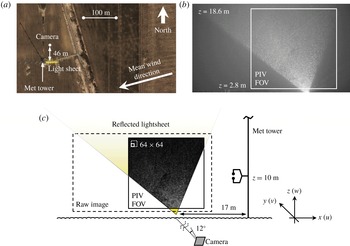
The field measurements were collected at the University of Minnesota Eolos Wind Research Field Station in Rosemount, Minnesota. The field deployment occurred in the early morning of 11 December 2016 between 00:30 and 02:00 central standard time. The area surrounding the measurement site is primarily flat farmland with trees and sparse two-storey buildings farther away. At the time of the deployment, the farmland was harvested such that the soil was overturned and short, cut vegetation protruded through the snow cover. The roughness of the overturned soil was evident through the shallow snow cover. Upwind of the measurement location, there is a shallow ditch with shrubs 100 m away followed by 1 km of flat farmland. The approximate height of the shrubs is less than 1 m. A meteorological (met) tower is situated 17 m downwind of the imaging field. Aside from the met tower, the nearest downstream obstruction is a row of trees 200 m away. An aerial view of the site is shown in figure 1(a).
(a) Google Earth aerial image of the field site with enhanced brightness and contrast. (b) Example unfiltered image frame. (c) Schematic of the field deployment where the image within the cropped field of view (FOV) is an example background-subtracted frame.

Measurements from the met tower are used here to supplement the SLPIV results. The 130 m tall met tower has three CSAT3 sonic anemometers (heights
 $z=10$
, 30 and 80 m) and six cup-and-vane anemometers (heights
 $z=7$
, 27, 52, 77, 102 and 126 m). The sonic anemometers measure velocity in three directions as well as temperature at 20 Hz. The 1 Hz cup-and-vane anemometers are each paired with temperature and relative humidity sensors. Figure 1(c) shows the met tower and lowest sonic anemometer position with respect to the imaging set-up. Further details on the site and met tower are given in Hong et al. (Reference Hong, Toloui, Chamorro, Guala, Howard, Riley, Tucker and Sotiropoulos2014) and Toloui et al. (Reference Toloui, Riley, Hong, Howard, Chamorro, Guala and Tucker2014).
2.2 Particle image velocimetry
To illuminate the snow particles, we created a reflected lightsheet as shown in figure 1(c) using a 5 kW searchlight and a curved reflective panel. The lightsheet is approximately 0.3 m thick at its base and 0.4 m thick through the field of view (FOV). The lightsheet width (in
 $x$
) also increases with height (in
 $z$
), creating a non-rectangular imaging field. The lightsheet was oriented with the anticipated mean wind direction based on weather forecasts and current conditions measured by the met tower. The alignment of the sheet with respect to the mean wind is discussed further in § 3.1.1.
To achieve the desired FOV, the camera was tilted
 $12^{\circ }$
from the horizontal at a standoff distance of 46 m as shown in figure 1(a). Using a 50 mm Nikon lens, the Nikon D600 CMOS camera acquired full high-definition (2.1 megapixel) images at a 30 Hz frame rate. An example unfiltered image is shown in figure 1(b). Three image sets were captured, each approximately 15 min in duration.
The camera height, inclination and standoff distance determine the centre of the FOV, namely its height and its object distance from the camera. The magnification and corresponding pixel resolution at the FOV centre were calculated using the object distance and the thin lens formula, yielding a 17
 $\text{mm}~\text{pixel}^{-1}$
resolution. The pixel resolution is related to the magnification through the camera sensor resolution. Due to the inclination of the camera, the object distance from the camera to the lightsheet plane increases with increasing height, resulting in non-uniform magnification and resolution values. The FOV extent was determined based on the known FOV centre position and the resolution throughout the FOV. Following Toloui et al. (Reference Toloui, Riley, Hong, Howard, Chamorro, Guala and Tucker2014), the images were corrected to achieve a uniform 17
 $\text{mm}~\text{pixel}^{-1}$
resolution with the FOV centre as the anchored reference point. The pixel resolution and the FOV height was confirmed using a reference object with a known size and position at the FOV bottom. Despite the confirmation, we estimate the uncertainty in the calibrated resolution to be 0.7
 $\text{mm}~\text{pixel}^{-1}$
, assuming conservative uncertainties of 2 m in the camera standoff distance and
 $1^{\circ }$
in the tilt angle.
Following the magnification correction, the images were pre-processed using minimum intensity background subtraction and were masked to exclude non-illuminated areas, resulting in filtered images such as the inset image of figure 1(c). PIV cross-correlations on the filtered images were executed using an iterative adaptive correlation scheme (Nemes et al.
Reference Nemes, Jacono, Blackburn and Sheridan2015). The interrogation windows were
 $64\times 64~\text{pixel}^{2}$
in the first pass and
 $32\times 32~\text{pixel}^{2}$
in the second pass, with each pass employing 50 % overlap. The resulting vector field spacing is
 $\unicode[STIX]{x0394}x=0.27$
m. With a surface layer depth of order
 $\unicode[STIX]{x1D6FF}\sim O$
(100 m), the spatial resolution normalized in outer wall units is
 $\unicode[STIX]{x0394}x/\unicode[STIX]{x1D6FF}\sim 10^{-3}$
. This resolution is finer than previous field studies using met-mounted anemometers, and is also an improvement compared to many previous laboratory studies. The unprecedented resolution allows us to analyse the instantaneous structure of the log layer in novel ways which will be presented in the following sections.
Outlier vectors were detected and replaced using the criteria of Westerweel & Scarano (Reference Westerweel and Scarano2005). To exclude regions where the percentage of rejected vectors exceeded 10 %, the field of view was cropped to the extents shown in figure 1(b). To mitigate any effects of pixel locking which can bias UMZ analysis (de Silva et al. Reference de Silva, Hutchins and Marusic2016), we applied histogram equalization in post-processing following Roth & Katz (Reference Roth and Katz2001). We performed the equalization separately for each position in the vector field (Hearst & Ganapathisubramani Reference Hearst and Ganapathisubramani2015).
We estimate the measurement uncertainty of the velocity vectors considering separately the
 $0.7~\text{mm}~\text{pixel}^{-1}$
resolution uncertainty and a nominal pixel displacement uncertainty of 0.2 pixels, leading to
 $0.1~\text{m}~\text{s}^{-1}$
uncertainty for each vector. We estimate the statistical uncertainty using 95 % confidence bounds. We calculate the total uncertainty as the magnitude of the measurement and statistical uncertainties. Uncertainty ranges for parameters such as
 $U_{\unicode[STIX]{x1D70F}}$
are discussed in the text and reflected in later figures using error bars.
The PIV results yield a non-zero mean wall-normal velocity due to the settling velocity of the snow
 $W_{s}$
. The true mean wall-normal velocity is assumed to be zero such that the measured mean velocity is equal to the settling velocity
 $W=W_{s}\approx 1.3~\text{m}~\text{s}^{-1}$
. Instantaneous velocities are then decomposed from the settling velocity as
 $w(x,z)=w_{piv}(x,z)-W_{s}(z)$
and the resulting velocities are treated as the turbulent fluctuations.
2.3 Snow particles as passive tracers
While the properties of snow particles as PIV flow tracers have been discussed for previous snow SLPIV experiments (Hong et al.
Reference Hong, Toloui, Chamorro, Guala, Howard, Riley, Tucker and Sotiropoulos2014; Toloui et al.
Reference Toloui, Riley, Hong, Howard, Chamorro, Guala and Tucker2014), the quality of snow particles is dependent on weather conditions. We therefore revisit the discussion here in consideration of the specific deployment conditions. Using digital in-line holography (see Nemes et al.
Reference Nemes, Dasari, Hong, Guala and Coletti2017) and fresh snow samples from the ground for verification, we identified the snowflakes as individual ice crystals in the shape of plates. The hexagonal prism is the most basic ice crystal structure, and these prisms form plates when the preferential growth direction favours the hexagonal face (Pruppacher & Klett Reference Pruppacher and Klett1997). Plates occur when temperatures are within the range
 $-9\,^{\circ }\text{C}$
to
 $-22\,^{\circ }\text{C}$
(Pruppacher & Klett Reference Pruppacher and Klett1997), which is consistent with the air temperature
 $-10^{\circ }$
to
 $-11\,^{\circ }\text{C}$
measured by the met tower during the deployment. Images and sizes of 196 snowflakes were captured using the holography. The average size of the crystals is described by the face diameter
 $D_{p}=0.61$
mm and the thickness
 $H_{p}=0.25$
mm.
Various models exist to estimate the bulk density of ice crystals. Most models follow a power law relationship
 $\unicode[STIX]{x1D70C}_{p}=aD_{p}^{b}$
, where
 $a=$
100 to 200,
 $b=-0.9$
to
 $-1$
,
 $D_{p}$
is the diameter in mm and
 $\unicode[STIX]{x1D70C}_{p}$
is the bulk density in
 $\text{kg}~\text{m}^{-3}$
(Brandes et al.
Reference Brandes, Ikeda, Zhang, Schönhuber and Rasmussen2007). Using the suggested values for
 $a$
and
 $b$
from three recent references, our estimated bulk density is
 $\unicode[STIX]{x1D70C}_{p}=167$
, 213 or 281
 $\text{kg}~\text{m}^{-3}$
(Heymsfield et al.
Reference Heymsfield, Bansemer, Schmitt, Twohy and Poellot2004; Brandes et al.
Reference Brandes, Ikeda, Zhang, Schönhuber and Rasmussen2007; Thompson et al.
Reference Thompson, Field, Rasmussen and Hall2008, respectively). We assume the true density was within the range of these estimates, and use the limits to approximate the uncertainty bounds as
 $\unicode[STIX]{x1D70C}_{p}=167$
–281
 $\text{kg}~\text{m}^{-3}$
.
To estimate the response time of the snow particles, we apply the standard Stokes drag relationship with a correction for finite particle Reynolds number
 $Re_{p}=W_{s}D_{p}/\unicode[STIX]{x1D708}$
. The corrected formula is
 $\unicode[STIX]{x1D70F}_{p}=\unicode[STIX]{x1D70C}_{p}D_{p}^{2}/18\unicode[STIX]{x1D707}(1+0.15Re_{p}^{0.687})$
, where
 $\unicode[STIX]{x1D707}$
is the dynamic viscosity of air (Crowe et al.
Reference Crowe, Schwarzkopf, Sommerfeld and Tsuji1998). The drag correction assumes a solid spherical particle. This assumption can underestimate the snowflake drag and overestimate the particle response time as suggested by Nemes et al. (Reference Nemes, Dasari, Hong, Guala and Coletti2017). However, in the absence of an accurate drag coefficient estimate, we use the corrected drag formula above and treat the formula as conservative. We also assume the hexagonal face is always normal to the flow such that the projected area is maximized. Based on the average measured snow settling velocity and the density range given above, the particle Reynolds number is
 $Re_{p}=62$
and the range of particle response time is
 $\unicode[STIX]{x1D70F}_{p}=0.056$
–0.095 s.
For the flow time scale, the limiting case relevant to the PIV calculations is
 $\unicode[STIX]{x1D70F}_{f}=l/\unicode[STIX]{x1D70E}_{u}$
, where
 $l=0.54$
m is the final interrogation window size and
 $\unicode[STIX]{x1D70E}_{u}=0.6~\text{m}~\text{s}^{-1}$
is the maximum measured streamwise root-mean-square (r.m.s.) velocity. The limiting measurement time scale is therefore
 $\unicode[STIX]{x1D70F}_{f}=0.9$
s. The corresponding particle Stokes number range is
 $St=\unicode[STIX]{x1D70F}_{p}/\unicode[STIX]{x1D70F}_{f}=0.06$
–0.11, making the snow particles reasonable tracers for our selected interrogation window size. Later results provide further verification of the snow particle traceability: the SLPIV measurement capture well the first- and second-order velocity statistics, and the values of
 $\unicode[STIX]{x1D70E}_{u}$
from the SLPIV and sonic anemometer measurements at
 $z=10$
m match to within 6 %.
3 Site conditions and velocity profiles
3.1 Atmospheric effects
The primary challenge in studying atmospheric turbulence is identifying and accounting for meteorological scales and other weather effects. These effects, discussed in the sub-sections below, include time-varying mean wind conditions and thermal stability.
3.1.1 Wind direction
The reflected lightsheet was aligned with the mean wind direction at the onset of the deployment, but changes in the direction resulted in mean out-of-plane velocities. With the lightsheet oriented at
 $90^{\circ }$
(clockwise from north), the average wind directions listed in table 1 result in misalignments of
 $16^{\circ }$
,
 $18^{\circ }$
and
 $13^{\circ }$
for the respective SLPIV data periods. A time series of the wind direction from 1 Hz met tower measurements at
 $z=7$
m is shown in figure 2(a).
Extended time series of atmospheric conditions as measured by 1 Hz met tower sensors. (a) A 1-min moving average of the wind direction
 $\unicode[STIX]{x1D6FD}$
relative to the lightsheet orientation at
 $z=7$
m. (b) Horizontal wind speed
 $U$
space–time contour. (c) Virtual potential temperature
 $\unicode[STIX]{x1D703}_{v}$
space–time contour. The three SLPIV data periods are outlined by the numbered boxes. The contour plots in (b,c) were interpolated from 10-min moving averages at the six measurements altitudes shown in the vertical axes. The blue dashed lines in (b,c) represent the top height of the SLPIV FOV.

Overview of atmospheric conditions during the three SLPIV measurement periods. Wind speed
 $U$
and direction
 $\unicode[STIX]{x1D6FD}$
are averages for the period listed based on 20 Hz sonic anemometer measurements at
 $z=10$
m. The local flux Richardson values
 $R_{f}$
are based on measurements at the listed heights.

To quantify possible out-of-plane effects on the PIV correlations, we consider here the wind direction and speed listed in table 1 for data set 2, which has the largest misalignment between the lightsheet and the mean wind. The mean wind speed and
 $18^{\circ }$
misalignment result in a
 $1.4~\text{m}~\text{s}^{-1}$
out-of-plane velocity. Based on the 0.4 m thickness of the lightsheet and 30 Hz sampling rate, the mean expected residence time of particles in the lightsheet is 8 frames. We do not expect particles entering and exiting the lightsheet plane to significantly impact the correlations because a majority of particles remain in the plane for numerous frames.
To calculate velocity statistics, we rotated the met tower measurements into the mean wind direction. We also projected the SLPIV streamwise velocities onto the mean wind direction to compensate for misalignment. As an example, the compensation for the mean velocity of SLPIV data set 2 is an approximate 5 % increase:
 $\cos (18^{\circ })^{-1}=1.05$
. The mean velocity projection uses the fact that the corrected mean spanwise velocity is zero. The projection is applied only for the velocity profiles in this section (§ 3). The results of our later analysis rely on turbulence statistics and instantaneous vector values for which we cannot assume the corrected spanwise component to be zero. Rather than attempt any projection, results after § 3 are based on the original lightsheet orientation. We acknowledge that the misalignment may underestimate streamwise-oriented statistics up to 5 % and we incorporate this effect in our estimated uncertainties.
3.1.2 Convergence
We use statistical convergence to evaluate variations in the mean wind conditions and the duration of the SLPIV data periods. Statistics will not converge if either the mean conditions change (i.e. non-stationarity) or if an insufficient number of very-large-scale turbulent events are recorded. Figure 3 depicts the statistical convergence for the three data periods using sonic anemometer measurements at
 $z=10$
m. The slowly increasing mean velocities in figure 3(a), most noticeably for data sets 2 and 3, indicate slowly varying wind conditions. To account for the increasing mean, the streamwise velocity fluctuations of the met tower and SLPIV data are calculated by subtracting a linear slope from the velocity series rather than a single time-averaged mean.
Statistical convergence of the velocity variances, based on the linear detrending, are shown in figure 3(b–d). The streamwise and wall-normal variances in figure 3(b,c) are well converged. The effect of large-scale motions on the Reynolds shear stress is visible in figure 3(d), where the average value for
 $-\overline{uw}$
is still fluctuating after 10 min. While the shear stress data do not appear fully converged due to the limited number of large-scale events, the changes in
 $-\overline{uw}$
for data set 1 are less than 4 % in the final two minutes of the acquisition period.
Convergence of velocity statistics for SLPIV data periods 1 (—
 $\!$
—), 2 (– –) and 3
 $(\cdots )$
based on sonic anemometer measurements at
 $z=10$
m projected onto the mean wind direction. (a) The mean velocity
 $U$
. (b) The streamwise variance
 $\overline{uu}$
. (c) The wall-normal variance
 $\overline{ww}$
. (d) The Reynolds shear stress
 $-\overline{uw}$
.

3.1.3 Thermal stability
Met tower measurements were used to estimate the thermal stability with the local flux Richardson number
 $R_{f}$
. The flux Richardson number is the ratio of buoyancy production to shear production of turbulence and is defined as
 $$\begin{eqnarray}R_{f}=\frac{{\displaystyle \frac{g}{\overline{\unicode[STIX]{x1D703}_{v}}}}\overline{w\unicode[STIX]{x1D703}_{v}}}{\overline{uw}{\displaystyle \frac{\unicode[STIX]{x2202}U}{\unicode[STIX]{x2202}z}}},\end{eqnarray}$$
where
 $g$
is the gravitational constant and
 $\unicode[STIX]{x1D703}_{v}$
is the virtual potential temperature in Kelvin. The virtual potential temperature is the temperature that dry air at standard atmospheric pressure must have to equal the density of air described by a given temperature, moisture content and pressure. Removing the effects of moisture and pressure allows for
 $\unicode[STIX]{x1D703}_{v}$
to replace density in the buoyancy production term above (Stull Reference Stull1988). In the log layer, the mean shear is
 $\unicode[STIX]{x2202}U/\unicode[STIX]{x2202}z=U_{\unicode[STIX]{x1D70F}}/\unicode[STIX]{x1D705}z$
, where
 $\unicode[STIX]{x1D705}$
is the von Kármán constant. The flux Richardson number is then equivalent to the Monin–Obukhov stability parameter
 $\unicode[STIX]{x1D701}=z/L$
near the surface (i.e.
 $z=10$
m), where
 $L$
is the Obukhov length
 $L=-U_{\unicode[STIX]{x1D70F}}^{3}\overline{\unicode[STIX]{x1D703}_{v}}/\unicode[STIX]{x1D705}g\overline{w\unicode[STIX]{x1D703}_{v}}$
based on surface measurements. To estimate
 $R_{f}$
, we approximated the turbulent virtual potential heat flux as
 $\overline{wT}$
. The heat and momentum fluxes were estimated using detrended 20 Hz sonic anemometer measurements. The average virtual potential temperature
 $\overline{\unicode[STIX]{x1D703}_{v}}$
was calculated using 1 Hz temperature, pressure and relative humidity measurements. Determination of the shear velocity
 $U_{\unicode[STIX]{x1D70F}}$
is described in § 3.2.
When the magnitude of
 $R_{f}$
at the surface is small (
 $|R_{f}|=|\unicode[STIX]{x1D701}|\lesssim 0.1$
, Högström, Hunt & Smedman Reference Högström, Hunt and Smedman2002), buoyancy effects are considered negligible and the surface layer stability is classified as near-neutral. For larger
 $R_{f}$
values the surface layer is either stable (
 $R_{f}>0$
) or unstable (
 $R_{f}<0$
).
The resulting
 $R_{f}$
values at the three sonic anemometer heights are given in table 1. The values are consistent with the potential temperature
 $\unicode[STIX]{x1D703}_{v}$
space–time contour in figure 2(c): stability conditions at the surface are near-neutral where
 $\unicode[STIX]{x2202}\unicode[STIX]{x1D703}_{v}/\unicode[STIX]{x2202}z$
is flatter.
 $\unicode[STIX]{x2202}\unicode[STIX]{x1D703}_{v}/\unicode[STIX]{x2202}z$
becomes increasingly negative with increasing height and the
 $R_{f}$
values indicate increasing stability. Despite indications of near-neutral stability at the surface, we acknowledge potential effects of a weakly stable surface layer. The
 $R_{f}(z)$
trends appear consistent between the three data periods, but the effects of stability may not be equal. The space–time contour of wind speed in figure 2(b) shows an extended period of relatively constant (low-pass filtered) wind speed at the second measurement height (
 $z=27$
m) between 23:00 and 01:00 local time. Beginning at 01:00, wind speed increases as motions of the order of 45–60 min are apparent in the contours throughout the remainder of the morning. These motions, possibly gravity waves associated with stable surface layers, appear to propagate down to the
 $z=27$
m measurement height. From the visual evidence in figure 2(b) we therefore identify a higher potential for thermal stability effects in SLPIV data sets 2 and 3.
3.2 The rough wall log layer
3.2.1 Velocity mean
The log layer, more formally known as the inertial sublayer or logarithmic region, occurs above the roughness sublayer for rough wall boundary layers. The mean streamwise velocity
 $U$
follows the profile
 $$\begin{eqnarray}U^{+}=\frac{1}{\unicode[STIX]{x1D705}}\log z^{+}+A-\unicode[STIX]{x0394}U^{+},\end{eqnarray}$$
where
 $A$
is the smooth wall constant and
 $\unicode[STIX]{x0394}U^{+}$
is the roughness function;
 $\unicode[STIX]{x0394}U^{+}$
describes the bulk velocity deficit due to surface roughness. In a series of experiments with sandpaper roughness, Nikuradse (Reference Nikuradse1933) developed the relationship
 $$\begin{eqnarray}\unicode[STIX]{x0394}U^{+}=\frac{1}{\unicode[STIX]{x1D705}}\log k_{s}^{+}+A-A_{FR},\end{eqnarray}$$
where
 $k_{s}^{+}$
is the equivalent sand grain roughness normalized in inner wall units and
 $A_{FR}=8.5$
is the fully rough constant. Equation (3.3) is true regardless of the roughness geometry if the flow conditions are within the fully rough regime (
 $k_{s}^{+}\gtrsim 70$
, Jiménez Reference Jiménez2004). The value of
 $k_{s}$
does not represent the physical roughness, but is rather the sand grain size required to achieve an equivalent
 $\unicode[STIX]{x0394}U^{+}$
. The relationship between
 $k_{s}$
and the physical roughness length
 $k$
is dependent on the roughness geometry.
Combining (3.2) and (3.3) yields the alternate form
 $U^{+}=\unicode[STIX]{x1D705}^{-1}\log z/k_{s}+A_{FR}$
for fully rough conditions. The common form of the mean velocity equation in micrometeorology is
 $U^{+}=\unicode[STIX]{x1D705}^{-1}\log z/z_{o}$
, where the aerodynamic roughness length
 $z_{o}$
is related to the equivalent roughness as
 $z_{o}=0.033k_{s}$
for fully rough conditions.
 $z_{o}$
describes the wall-normal displacement of the log layer due to surface roughness.
 $\unicode[STIX]{x0394}U$
and
 $z_{o}$
therefore both characterize the effect of roughness, with
 $\unicode[STIX]{x0394}U$
displacing velocity and
 $z_{o}$
displacing the wall-normal position.
To compare our velocity profiles with theory, we use the velocity statistics projected onto the mean wind direction. As discussed, we subtract the snow settling from the SLPIV vertical velocities and linearly detrend the horizontal velocities to estimate turbulent fluctuations. The compensated mean velocity profile for the three data sets, following the form of (3.2), is shown in figure 4(a). Profiles from rough wall wind tunnel studies (Krogstad, Antonia & Browne Reference Krogstad, Antonia and Browne1992; Flack, Schultz & Connelly Reference Flack, Schultz and Connelly2007; Schultz & Flack Reference Schultz and Flack2007; Squire et al. Reference Squire, Morrill-Winter, Hutchins, Schultz, Klewicki and Marusic2016b ; Morrill-Winter et al. Reference Morrill-Winter, Squire, Klewicki, Hutchins, Schultz and Marusic2017) as well as atmospheric studies at the SLTEST (Kunkel & Marusic Reference Kunkel and Marusic2006; Hutchins et al. Reference Hutchins, Chauhan, Marusic, Monty and Klewicki2012) and QLOA (Wang & Zheng Reference Wang and Zheng2016) facilities are included for reference. Additional atmospheric measurements from met-mounted anemometers (Clarke et al. Reference Clarke, Dyer, Brokk, Reid and Troup1971; Tieleman Reference Tieleman2008) are also included.
Normalized streamwise mean velocity profiles for the three data sets compared with selected results of laboratory (grey filled symbols) and atmospheric (black filled symbols) studies. The wall-normal position is normalized using (a) inner wall units and (b) the aerodynamic roughness length. Reference lines in (a) for smooth wall (– –), transition to fully rough (—
 $\!$
—) and the present data
 $(\cdots )$
have slope
 $\unicode[STIX]{x1D705}^{-1}$
where
 $\unicode[STIX]{x1D705}=0.39$
. Symbols for the SLPIV (black), sonic (red) and cup (blue) data are defined in table 2. Every fourth SLPIV data point is shown for clarity. Transparent points are outside the region exhibiting log–linear behaviour.

For the current data, we observe the expected log–linear increase in mean velocity up to approximately
 $z=70$
m. The log–linear range is captured by the SLPIV (black markers), sonic anemometers (red) and cup and vane anemometers (blue). The upper limit of the range is somewhat arbitrary due to the low spatial resolution of the met tower. The fully rough cases shown in figure 4(a), including the current data, are re-plotted in figure 4(b) with the wall-normal position normalized by
 $z_{o}$
. Only the fully rough cases are included here because
 $z_{o}$
can be calculated directly from the
 $k_{s}$
values reported in the cited literature for fully rough studies.
The parameters used to normalize our velocity profiles, namely the shear velocity
 $U_{\unicode[STIX]{x1D70F}}$
and roughness parameters, are listed in table 2. Separate values of
 $U_{\unicode[STIX]{x1D70F}}$
for each data set were determined manually by collapsing the velocity profiles of the three sets and aligning the slope of the mean velocity with
 $\unicode[STIX]{x1D705}^{-1}$
as shown in figure 4(a). The selection of the
 $U_{\unicode[STIX]{x1D70F}}$
values also considered the theoretical Reynolds shear stress peak
 $-\overline{uw}_{max}^{+}\approx 1$
. A least-squares fit of the profiles was not employed to define
 $U_{\unicode[STIX]{x1D70F}}$
due to the fact that multiple profiles and conditions were considered simultaneously. Because we considered the Reynolds shear stress in the determination of
 $U_{\unicode[STIX]{x1D70F}}$
, we approximated the
 $\pm 0.03~\text{m}~\text{s}^{-1}$
(10 %) uncertainty bounds for
 $U_{\unicode[STIX]{x1D70F}}$
based on the experimental and convergence uncertainty for
 $-\overline{uw}_{max}$
.
With
 $U_{\unicode[STIX]{x1D70F}}$
defined for each data set, a single value for the aerodynamic roughness length
 $z_{o}$
(
 $k_{s}$
) was determined. Because the conditions are well within the fully rough regime,
 $z_{o}$
and
 $k_{s}$
depend only on the surface geometry and do not change between data sets.
 $z_{o}$
was calculated using a nonlinear least-squares fit of all the mean velocity data points up to
 $z=70$
m to achieve the alignment shown in figure 4(b). The excellent collapse of the data along the theoretical line validates the values of
 $U_{\unicode[STIX]{x1D70F}}$
and
 $z_{o}$
(
 $k_{s}$
) for both our data and the cited studies.
Surface scaling parameters for the field site characterized by farmland with overturned soil, shallow snow cover and protruding vegetation. The conversion
 $z_{o}=0.033k_{s}$
for fully rough flows is used. The approximated Reynolds number uses a surface layer depth uncertainty range
 $\unicode[STIX]{x1D6FF}=70$
–200 m.

3.2.2 Velocity variance
The conceptual arguments of Townsend (Reference Townsend1976) lead to the profiles for the second-order velocity statistics. Specifically, the streamwise variance profile in the log layer is
 $\overline{u^{2}}^{+}=B_{1}-A_{1}\log (z/\unicode[STIX]{x1D6FF})$
where
 $A_{1}$
and
 $B_{1}$
are constants, and the wall-normal variance profile is
 $\overline{w^{2}}^{+}=C_{1}$
where
 $C_{1}$
is a constant (Townsend Reference Townsend1976). The Reynolds shear stress profile is
 $-\overline{uw}^{+}\approx 1$
. Verification of the velocity profile equations and the values for the constant parameters has been the subject of many studies, including those summarized in Marusic et al. (Reference Marusic, Monty, Hultmark and Smits2013). Certain constants, including
 $B_{1}$
, are expected to be dependent on the surface roughness (Squire et al.
Reference Squire, Morrill-Winter, Hutchins, Schultz, Klewicki and Marusic2016b
).
The variance profiles for the three data sets are shown in figure 5 with the same literature results as the mean velocity included for comparison. We observe the expected log–linear decrease in streamwise variance beginning at
 $z=5.5$
m (
 $z^{+}=2.2\times 10^{5}$
). Together with the agreement between our mean velocity profiles and (3.2) up to
 $z=70$
m, the log–linear behaviour of
 $\overline{u^{2}}^{+}$
suggests a log layer from
 $z=5.5$
to 70 m. Points outside this range are shown with transparency in figures 4 and 5.
Turbulent velocity profiles normalized with inner wall units for the three data sets and selected literature results. (a) The streamwise variance
 $\overline{uu}^{+}$
. (b) The wall-normal variance
 $\overline{ww}^{+}$
. (c) The Reynolds shear stress
 $\overline{uw}^{+}$
. Literature symbols are defined in the figure 4 legend. Symbols for the SLPIV (black) and sonic (red) data are defined in table 2. Every fourth SLPIV data point is shown for clarity. Transparent points are outside the region exhibiting log–linear behaviour.

The peak values in each of the variances profiles of figure 5 are also in agreement with the previous literature. In particular, the streamwise variance in figure 5(a) and wall-normal variance in figure 5(b) are consistent with other field measurements. A noteworthy deviation from the theoretical profile is the decline in Reynolds shear stress seen in figure 5(c). We discuss this discrepancy and provide a more precise extent of the canonical log layer in § 7.4.
Velocity statistics computed for the SLPIV and sonic anemometer are in close agreement for the mean velocity, but the turbulence estimated by the sonic is lower. Compared to the SLPIV r.m.s. velocities at
 $z=10$
m, the sonic anemometer streamwise r.m.s velocity is
 $0.1~\text{m}~\text{s}^{-1}$
(6 %) lower and the wall-normal r.m.s. velocity is almost
 $0.3~\text{m}~\text{s}^{-1}$
(27 %) lower for data set 1. The large wall-normal r.m.s. velocity difference may be responsible for the difference in Reynolds shear stress. The CSAT3 sonic anemometers have a sample volume almost three times smaller in each direction than the SLPIV vector spacing, but the sampling frequency is 50 % slower. At
 $z=10$
m, more than 95 % of turbulent energy is at frequencies lower than the 10 Hz maximum frequency that the sonic can resolve (based on sonic velocity spectra extrapolated to the Kolmogorov scale using a
 $-5/3$
power law fit). The lower sampling frequency of the sonic also cannot explain the discrepancy between the underestimates of the streamwise and wall-normal r.m.s. velocities (0.1 versus
 $0.3~\text{m}~\text{s}^{-1}$
lower than SLPIV, respectively). The discrepancy may be explained by a combination of the snow precipitation and icing conditions (Makkonen, Lehtonen & Helle Reference Makkonen, Lehtonen and Helle2001), the non-orthogonality of the sonic anemometer (Frank, Massman & Ewers Reference Frank, Massman and Ewers2013) and the flow distortion from the met tower mast mount (Grant & Watkins Reference Grant and Watkins1989). Each of these has been shown to produce underestimates and errors in the vertical velocity measurements. Despite the potential underestimation of variances by the sonic anemometers, we see strong agreement between the normalized SLPIV data and literature values for the turbulence profiles.
3.3 Surface roughness
From the parametrization of the velocity profiles described in the previous section, the estimated aerodynamic roughness length for the site is
 $z_{o}=0.04$
m. This value is within the expected range
 $z_{o}=0.01$
–0.05 m for farmland (Stull Reference Stull1988; Garratt Reference Garratt1994). Because the snow cover was shallow and had not concealed the underlying roughness, the surface asperities from the overturned soil account for some of the aerodynamic roughness. The roughness values
 $\unicode[STIX]{x0394}U^{+}$
and
 $z_{o}$
then correspond to a combination of the asperities and protruding vegetation, where the vegetation is consistent with early wheat of roughness height
 $h=0.4$
m (Raupach, Antonia & Rajagopalan Reference Raupach, Antonia and Rajagopalan1991).
From the velocity variance profiles in figure 5, the far-wall variance peak occurs around
 $z=5.5$
m. The near-wall peak would be below the field of view, but is very likely not present due to destruction by the roughness elements (Grass Reference Grass1971; Schultz & Flack Reference Schultz and Flack2007; Squire et al.
Reference Squire, Morrill-Winter, Hutchins, Schultz, Klewicki and Marusic2016b
). The region below the far-wall peak is presumed to be the roughness sublayer. The peak occurs somewhat beyond the
 $3h$
(
 ${\approx}2$
m) and 5
 $k_{s}$
(
 ${\approx}3.6$
m) limits suggested by Flack et al. (Reference Flack, Schultz and Connelly2007), but the sublayer extent depends on the specific roughness geometry and the agreement is reasonable considering the disparity in flow scales between the present work and the cited study.
3.4 Length scales
To characterize the smallest flow scales, we assume production and dissipation are of the same order and use 10 m as a nominal height within the SLPIV field of view. The resulting Kolmogorov length scale is
 $\unicode[STIX]{x1D702}=(\unicode[STIX]{x1D708}/\unicode[STIX]{x1D716})^{1/4}\approx 0.7$
mm.
The surface layer depth
 $\unicode[STIX]{x1D6FF}$
is largely unknown for the Eolos field site. Because the surface layer definition is analogous to the logarithmic region of the conventional boundary layer (see § 1), a conservative estimate for the depth is
 $\unicode[STIX]{x1D6FF}_{min}\approx 70$
m, the approximate height at which the mean velocity deviates from log–linear behaviour in figure 4. We can also estimate the depth following the traditional laboratory-scale definition which uses the free-stream condition. Because the free-stream velocity is not reached by the top of the met tower (
 $z=130$
m) based on the mean velocities in figure 4, we choose a nominal maximum estimate
 $\unicode[STIX]{x1D6FF}_{max}\approx 200$
m. The SLPIV measurements are well within the log layer regardless of the uncertainty range
 $\unicode[STIX]{x1D6FF}=70$
–200 m. The Reynolds number range resulting from the
 $\unicode[STIX]{x1D6FF}$
estimate is
 $Re_{\unicode[STIX]{x1D70F}}\approx 2{-}5\times 10^{6}$
, which is comparable to other atmospheric studies (Kunkel & Marusic Reference Kunkel and Marusic2006; Hutchins et al.
Reference Hutchins, Chauhan, Marusic, Monty and Klewicki2012; Wang & Zheng Reference Wang and Zheng2016).
3.5 Data selection
For the remainder of the manuscript, we focus our analysis on data set 1; results presented in later sections are for data set 1 only. We prioritize set 1 due to the abundance of data (
 ${\approx}$
25 000 SLPIV frames per set) and observed variations in the site conditions. Set 1 has the steadiest conditions with respect to potential thermal stability effects (see figure 2(b) and § 3.1.3) and time-varying mean wind conditions (see figure 3(a) and § 3.1.2). Further, velocity variance profiles for set 1 (figure 5) exhibit the least variability near the top of the SLPIV field (
 $z^{+}\approx 5\times 10^{5}$
). We therefore infer data set 1 to most closely represent a canonical rough wall boundary layer.
4 Evidence of ramp-like structures
4.1 Visual evidence: vector fields
With the relatively fine two-dimensional spatial resolution of the current data set, we use instantaneous vector fields to identify the same structural features seen in previous laboratory-scale PIV studies. In particular, we replicate here the visual realization of Adrian et al. (Reference Adrian, Meinhart and Tomkins2000b
) to detect spanwise vortices in the streamwise–wall-normal plane. An example realization from an SLPIV frame in data set 1 is shown in the figure 6(a) vector field. To highlight the vortices and make their circular core apparent, we subtracted a convective velocity
 $U_{c}$
approximately equal to the local velocity of the vortices. The vector field shares the same signatures as the hairpin vortices in figures 10 and 11 of Adrian et al. (Reference Adrian, Meinhart and Tomkins2000b
): the vortices are at the head of a forward-inclined shear layer. The shear layer and vortices are being convected at the same speed. The shear layer separates a
 $Q$
2 (ejection) event from below and a
 $Q$
4 (sweep) event from above. The shear layer and the aligned spanwise vortices are inclined approximately
 $35^{\circ }$
from the horizontal. To more clearly identify the vortices, figure 6(b) shows a colour plot of the two-dimensional swirling strength
 $\unicode[STIX]{x1D706}_{ci}$
, where the sign of
 $\unicode[STIX]{x1D706}_{ci}$
is based on the out-of-plane vorticity
 $\unicode[STIX]{x1D714}_{y}$
. The regions of negatively signed swirl indicate prograde vortices. A movie showing the time evolution of the figure 6(a) vector field is included in the supplementary materials (see supplementary movie https://doi.org/10.1017/jfm.2018.759).
Realization of a vortex structure having the signature of a hairpin vortex packet with four vortex heads along an inclined shear layer. (a) Vortex signatures with elements labelled as in figure 11 of Adrian et al. (Reference Adrian, Meinhart and Tomkins2000b
). (b) Identification of the vortex heads by the swirling strength
 $\unicode[STIX]{x1D706}_{ci}$
. (c) Visualized zones of uniform momentum following figure 14 of Adrian et al. (Reference Adrian, Meinhart and Tomkins2000b
). (d) Normalized histogram of streamwise velocities for vectors within the dashed box of (c). Quiver plot reference frames in (a,c) use the convective velocity
 $W_{c}=-1~\text{m}~\text{s}^{-1}$
and the listed
 $U_{c}$
. The shear layer line in (a–c) is a contour of
 $u=3.75~\text{m}~\text{s}^{-1}$
, the minimum occurrence velocity as seen in (d).

Given the presence of multiple vortex heads along the single shear layer in figure 6(a), the signature resembles the hairpin vortex packet rather than the individual hairpin vortex. The hairpin packet signature has been observed for rough wall boundary layers in previous laboratory-scale studies (see e.g. Volino et al.
Reference Volino, Schultz and Flack2007; Hong, Katz & Schultz Reference Hong, Katz and Schultz2011). Despite the striking similarities between the vortex structure and a hairpin packet in the
 $x{-}z$
plane, we lack the necessary out-of-plane measurements to definitively remark on the three-dimensional shape of the vortex structure. We therefore limit our interpretation of figure 6(a,b) to an inclined vortex structure extending up to
 $z=12$
m and having features similar to hairpin packets previously observed in laboratory studies.
4.2 Statistical evidence: two-point correlations
Similar to the many studies cited in the introduction, we employ the two-point correlation here to assess the statistical importance of the inclined vortex structures. We look specifically at correlations of the streamwise velocity fluctuations. For a given reference height
 $z_{ref}$
, the two-point correlation
 $\unicode[STIX]{x1D70C}_{uu}$
is defined at each height
 $z$
and streamwise separation distance
 $r_{x}$
as
 $$\begin{eqnarray}\unicode[STIX]{x1D70C}_{uu}(r_{x},z,z_{ref})=\frac{\langle u^{\prime }(x,z_{ref})u^{\prime }(x+r_{x},z)\rangle }{\unicode[STIX]{x1D70E}_{u}(z_{ref})\unicode[STIX]{x1D70E}_{u}(z)},\end{eqnarray}$$
where
 $\unicode[STIX]{x1D70E}_{u}$
is the streamwise r.m.s. velocity and brackets (
 $\langle \cdot \rangle$
) indicate the average correlation across each
 $x$
position at the reference height. The resulting correlation contours for four reference heights are shown in figure 7. The well-correlated regions are elongated along the streamwise direction and inclined at a shallow angle from the horizontal, both indicative of the statistical persistence of the ramp-like structures in our flow.
Two-point correlations of the streamwise velocity fluctuations
 $\unicode[STIX]{x1D70C}_{uu}$
for four reference heights: (a)
 $z_{ref}=5$
m, (b)
 $z_{ref}=10$
m, (c)
 $z_{ref}=13$
m and (d)
 $z_{ref}=16$
m. The thick line indicates the inclination angle
 $\unicode[STIX]{x1D6FE}$
of the contours. Contour lines start at
 $\unicode[STIX]{x1D70C}_{uu}=0.9$
and decrease in 0.1 intervals.

To determine the inclination angle
 $\unicode[STIX]{x1D6FE}$
of the spatial correlation, we fitted ellipses to each contour (using finer contour intervals than shown in figure 7), identified the major axis edge points for each ellipse, and used a least-squares linear fit to form a line through all the major axis points. A similar method was employed by Volino et al. (Reference Volino, Schultz and Flack2007). The line resulting from the linear fit and the line angle
 $\unicode[STIX]{x1D6FE}$
are included in figure 7. The uncertainty bounds given for each inclination angle represent the 95 % confidence interval of the fitted slope. The
 $\unicode[STIX]{x1D6FE}=12^{\circ }$
and
 $13^{\circ }$
inclination angles at lower positions (
 $z_{ref}=5$
m and 10 m, respectively) are in excellent agreement with the
 $10^{\circ }$
to
 $15^{\circ }$
range of numerous literature (see e.g. Adrian et al.
Reference Adrian, Meinhart and Tomkins2000b
; Volino et al.
Reference Volino, Schultz and Flack2007; Dennis & Nickels Reference Dennis and Nickels2011; Guala et al.
Reference Guala, Metzger and McKeon2011; Liu et al.
Reference Liu, Bo and Liang2017). This agreement further confirms that the signature of ramp-like structures is qualitatively similar, at least in the inclination, across a range of scales independent of surface roughness (Volino et al.
Reference Volino, Schultz and Flack2007; Squire et al.
Reference Squire, Morrill-Winter, Hutchins, Marusic, Schultz and Klewicki2016a
).
Farther from the wall, at
 $z_{ref}=13$
m and 16 m in figure 7(c,d), the elongated shape of the correlations is maintained, but we observe a decrease in the inclination angle. Volino et al. (Reference Volino, Schultz and Flack2007) observed a similar flattening in their outer region (
 $z/\unicode[STIX]{x1D6FF}>0.7$
) entirely above the wall-attached structures, but other studies found an increase in
 $\unicode[STIX]{x1D6FE}$
with increasing
 $z$
(Dennis & Nickels Reference Dennis and Nickels2011; Hutchins et al.
Reference Hutchins, Chauhan, Marusic, Monty and Klewicki2012; Squire et al.
Reference Squire, Morrill-Winter, Hutchins, Marusic, Schultz and Klewicki2016a
) due to a bulging of the structures (Dennis & Nickels Reference Dennis and Nickels2011). The discrepancy of our findings with the latter studies may be due to methodology. In Hutchins et al. (Reference Hutchins, Chauhan, Marusic, Monty and Klewicki2012) and Squire et al. (Reference Squire, Morrill-Winter, Hutchins, Marusic, Schultz and Klewicki2016a
), the inclination of higher positions is based on the shape of low-correlation contour lines conditional to a
 $z_{ref}$
nearer the wall (see e.g. figure 11 of Hutchins et al. (Reference Hutchins, Chauhan, Marusic, Monty and Klewicki2012)). In figure 11 of Dennis & Nickels (Reference Dennis and Nickels2011), a higher local
 $z_{ref}$
was used, but the increased inclination is mainly apparent from the tails of the correlation contours away from the reference point. Considering our field of view is restricted relative to the observed extent of the vortex structure in figure 6, we may not have sufficient separation distances to capture the statistical signature of the bulged structures.
We purposefully avoided normalizing the distances in figures 6 and 7 because the size scaling behaviour of ramp-like structures is not yet fully understood. The example inclined vortex structure in figure 6 and the region with
 $\unicode[STIX]{x1D6FE}=10^{\circ }$
–
 $15^{\circ }$
correlation inclinations in figure 7 both extend to
 $z\approx 10$
m, which normalizes in inner wall units to
 $z^{+}\sim O(10^{5})$
and in outer wall units to
 $z/\unicode[STIX]{x1D6FF}\sim O(10^{-1})$
. The wall-normal extent of the ramp-like structures is further discussed in § 7.4.
4.3 Inclined vortex structures and zones of uniform momentum
Another important feature of inclined vortex structures such as the realization in figure 6 is that the corresponding shear layer provides a boundary for UMZs (Meinhart & Adrian Reference Meinhart and Adrian1995; Adrian et al.
Reference Adrian, Meinhart and Tomkins2000b
). To reveal the distinct momentum regions separated by the shear layer in figure 6(a), we subtracted a new convective velocity
 $U_{c}$
equal to the speed of the low-momentum region. The vector field resulting from the new
 $U_{c}$
value is shown in figure 6(c). The vector field clearly shows a low- and high-momentum region below and above the shear layer, respectively. These regions can be identified statistically using a histogram of the streamwise velocities in the vector field (Adrian et al.
Reference Adrian, Meinhart and Tomkins2000b
). To avoid selection bias in our non-rectangular SLPIV field, we limit the vectors contributing to the histogram to the rectangular area outlined by the dashed box in figure 6(c). A histogram of the vectors within the dashed box is shown in figure 6(d). The speed of the zones is represented by the modes of the histogram distribution, called the modal velocities (Adrian et al.
Reference Adrian, Meinhart and Tomkins2000b
; de Silva et al.
Reference de Silva, Hutchins and Marusic2016). The edge of the zones, i.e. the shear layer, is represented statistically by the minimum occurrence velocity in the histogram. The strong instantaneous
 $\unicode[STIX]{x2202}u/\unicode[STIX]{x2202}z$
values defining the shear layer results in a limited number of vectors with velocities between the two velocity modes representing the zone speeds. The contour line representing the shear layer in figure 6(a–c) corresponds to the minimum occurrence velocity. UMZs are analysed in greater detail in the following section.
5 Tracking zones of uniform momentum
5.1 Histogram construction
To track the properties of UMZs, the two-dimensional representation in figure 6(c,d) must be extended to the temporal domain. The primary consideration is the extent of the velocity field used to construct each histogram, both in terms of scaling and statistical convergence. Limiting the histogram contributions to a rectangular field as shown in figure 6(c) results in 8 (streamwise) columns which span the 59 (vertical) rows. A single frame is not sufficient to properly converge the histogram as seen in figure 6(d). To reach convergence, we use the 8 central columns in the FOV across 15 SLPIV frames to construct each histogram. The number of vectors contributing to each bin is therefore
 $8\times 59\times 15\approx 7\times 10^{3}$
, similar to de Silva et al. (Reference de Silva, Hutchins and Marusic2016) and Laskari et al. (Reference Laskari, de Kat, Hearst and Ganapathisubramani2018). The histogram space–time contributions are visualized in figure 8(a): the full SLPIV field in space–time (dotted lines) is reduced to a 15-frame rectangular prism (thick black lines). The resulting histogram is shown in figure 8(b).
Illustration of the vector field contributions for each histogram used to detect UMZs. (a) The full SLPIV field in space–time (dotted lines) reduced to a 15-frame rectangular prism (thick black lines). (b) A histogram of the streamwise velocity vectors from the 15-frame rectangular prism in (a). (c) A histogram of velocity vectors from 550 frames, scaled in outer wall units. (d) A histogram of velocity vectors from a single frame and column, scaled in inner wall units. The three histograms begin at the same SLPIV frame. The conversion from frames to streamwise extent is
 ${\mathcal{L}}_{x}=U_{B}(\text{frames}/f_{s})$
where
 $U_{B}\approx 4~\text{m}~\text{s}^{-1}$
is the bulk mean velocity and
 $f_{s}$
is the sampling frequency.

The temporal extent of the 15-frame histogram contributions is 0.5 s. Using Taylor’s frozen turbulence hypothesis, the streamwise spatial extent can be approximated by multiplying this time to the bulk mean velocity
 $U_{B}\approx$
4
 $~\text{m}~\text{s}^{-1}$
, yielding
 ${\mathcal{L}}_{x}\approx 0.5U_{B}\approx 2$
m. The streamwise extent can be normalized as
 ${\mathcal{L}}_{x}/\unicode[STIX]{x1D6FF}\approx 0.03$
and
 ${\mathcal{L}}_{x}^{+}\approx 45\,000$
. Increasing
 ${\mathcal{L}}_{x}$
to scale with
 $\unicode[STIX]{x1D6FF}\approx$
70 m results in the figure 8(c) histogram based on 550 SLPIV frames. The low velocity modes seen in figure 8(b) are no longer present in the figure 8(c) histogram because many zones with different momentum contribute to the histogram. Considering the changes in the modal velocities,
 ${\mathcal{L}}_{x}$
should be small compared to the boundary layer depth to avoid filtering all but the largest zones, in agreement with de Silva et al. (Reference de Silva, Hutchins and Marusic2016).
If we limit
 ${\mathcal{L}}_{x}$
to a single SLPIV column and frame, i.e. the shortest possible for our data, the resulting length is
 ${\mathcal{L}}_{x}^{+}\approx 3000$
and the corresponding histogram is shown in figure 8(d). The value
 ${\mathcal{L}}_{x}^{+}\approx 3000$
is comparable to the value
 ${\mathcal{L}}_{x}^{+}=2000$
suggested by de Silva et al. (Reference de Silva, Hutchins and Marusic2016). The histograms in figure 8(b,d) exhibit some similar qualities such as the modes at 2.2 and
 $3.1~\text{m}~\text{s}^{-1}$
, but the short extent does not allow statistical convergence. We therefore use the larger
 ${\mathcal{L}}_{x}^{+}\approx 45\,000$
. Later results pertaining to the streamwise length of detected UMZs indicate that viscous and outer units are not the proper scaling parameter for
 ${\mathcal{L}}_{x}$
, and that an intermediate length scale is more appropriate. We discuss the intermediate scaling, including further justification for our
 ${\mathcal{L}}_{x}$
, in § 7.3.
In addition to the 15-frame temporal extent, we introduce further smoothing by including the 8 central columns in each frame as opposed to a more simple two-dimensional
 $z{-}t$
plane. We include the multiple columns to improve convergence without increasing too much the temporal extent. The inclusion and smoothing is at the expense of the smallest measurable UMZs whose histogram peak may be eliminated. The smoothing and convergence effects induced by the choice of
 ${\mathcal{L}}_{x}$
represent the primary uncertainty in our UMZ analysis. Sensitivity analysis of
 ${\mathcal{L}}_{x}$
and the histogram parameters yielded up to 30 % changes in the calculated average UMZ streamwise extent based on a 2000 frame sample. The analysis included halving the span to 7 frames (i.e. halving
 ${\mathcal{L}}_{x}$
) and doubling the span to 30 frames. We use the range
 $\pm 30\,\%$
to represent uncertainty in later UMZ results.
Besides the frame span, another important consideration for the histogram construction is the bin width. Our selected bin width,
 $0.1~\text{m}~\text{s}^{-1}$
, is the same as the experimental uncertainty in the velocity vectors. The bin width results in approximately 30 bins per histogram. The normalized bin width is 0.33
 $U_{\unicode[STIX]{x1D70F}}$
, which is comparable to the 0.5
 $U_{\unicode[STIX]{x1D70F}}$
width employed by Laskari et al. (Reference Laskari, de Kat, Hearst and Ganapathisubramani2018). De Silva et al. (Reference de Silva, Philip, Hutchins and Marusic2017) showed the streamwise velocity jump between vertically adjacent UMZs to be 1–2 times
 $U_{\unicode[STIX]{x1D70F}}$
. This jump corresponds approximately to the velocity difference between modes in the histogram. Our normalized bin width is therefore small enough to allow for the average mode-to-mode velocity difference to be separated by multiple histogram bins. As a result, we are able to detect adjacent UMZs as distinct modes in the histogram.
5.2 Tracking methodology
The following description provides a brief overview of the methodology employed to identify momentum zones using the histograms and track the UMZs in time. Local peaks in a given histogram were considered as distinct UMZ modes by a peak detection algorithm based on a calibrated set of parameters. The parameters include the minimum distance between two peaks (2 bins), the minimum peak height (0.05) and minimum peak prominence (0.05), where the prominence is the height difference between the peak and its neighbouring minima. Similar parameter values were used by Laskari et al. (Reference Laskari, de Kat, Hearst and Ganapathisubramani2018). From the detected peaks, the modal velocities were determined using a local three-point Gaussian fit of the peaks, and the edge velocities were determined using a three-point parabolic fit of the minima between peaks. The example histogram in figure 9(a) shows the detected modes and edge velocities.
To determine the edge height, the 8-column streamwise velocity time series was reduced to the central (fifth) column, resulting in a
 $z{-}t$
velocity series at the centre
 $x$
position. The UMZ edge heights were the
 $z$
position of the edge velocity contour(s) at the centre of the frame span as shown in figure 9(b). The bottom and top edge heights for a given zone speed were assigned by matching the zone speeds with the mean of the streamwise velocity vectors between each edge height (including the bottom and top of the field). The mode and edge detection was repeated by shifting forward one frame and computing the new histogram. Because the frame shift between histograms was shorter than the 15-frame span of the histogram construction, there was overlap in the vectors contributing to consecutive histograms. The effect of the vector overlap is quantified using the frame span sensitivity analysis discussed above.
Demonstration of the UMZ tracking methodology. (a) A streamwise velocity histogram with the detected modal (○) and zone edge velocities (
 $\times$
). (b) The velocity colour plot in space–time including the 15-frame histogram span (bounded by the dashed lines) and contours of the edge velocities from (a) which are used to detect the edge heights for
 $t=2.5$
s. (c) The detected UMZ modal velocities
 $U_{umz}$
in time where the histogram in (a) corresponds to
 $t=2.5$
s. (d) The definitions of zone average midheight
 $z_{umz}$
, total time duration
 $T_{umz}$
, wall-normal thickness
 $H_{umz}$
and height-dependent length
 $L_{umz}(z)=U_{umz}T_{umz}(z)$
. Blue lines and markers in each plot indicate attributes associated with the zone featured in (d).

Following the calculation of modal velocities and edge heights for every frame, the UMZs were tracked temporally using a nearest-neighbour routine, resulting in the tracked zone speeds in figure 9(c). The algorithm connected UMZ modes between frames if the modal velocity difference was less than 1.5 bin widths. The duration of the connected UMZ modes defines the extent of the zone. UMZs lasting only one frame were considered short-lived and were removed (Laskari et al.
Reference Laskari, de Kat, Hearst and Ganapathisubramani2018). The boundaries of each remaining UMZ were converted from scattered bottom and top heights to an enclosed shape as shown in figure 9(d). The velocity vectors belonging to each zone are those within the UMZ boundaries. Properties computed for each UMZ include those defined in figure 9(d): the average midheight
 $z_{umz}$
, total time duration
 $T_{umz}$
, wall-normal thickness
 $H_{umz}$
and height-dependent streamwise length
 $L_{umz}(z)=U_{umz}T_{umz}(z)$
. The height, thickness and duration properties are based on the position of the UMZ boundaries in the
 $z{-}t$
plane. The use of Taylor’s frozen turbulence hypothesis to convert the time duration to streamwise length is justified here due to the fact that each UMZ moves with a uniform velocity by definition.
A total of 1300 UMZs were identified from the tracking routine. Figure 10 provides results of the UMZ edge tracking routine for two 5-second sample periods. The interfaces align well with the shear identified in figure 10(c,d) and the vortices based on swirling strength in figure 10(e,f). However, the inherent requirement for a substantial number of velocity vectors in a given zone to manifest a histogram peak is apparent in two ways. First, it results in the inability to detect zones only partially in the field of view. For instance, the high shear at the bottom of the field in figure 10(d) indicates a potential zone interface, but insufficient vectors are present to detect the zone that likely appears just below the field of view. Second, an emerging zone may not immediately correspond to a histogram peak. When the zone is detected in these cases, the vertical extent of the UMZ is already substantial, leading to an apparent vertical front edge. This can be seen for both samples in figure 10(a,b) near
 $z=10$
m and
 $t=2.5$
s. The result of these limitations in the tracking methodology are potentially biased statistics near the top and bottom of the field as well as underestimated durations for certain UMZs to the favour of the surrounding zones. In consideration of the field edge effects, later figures and discussion of wall-normal UMZ trends clearly acknowledge the regions where bias is observed. We interpret the results using only the central region of the field where the statistics are most reliable. The underestimation of UMZ duration is discussed in § 5.3.
Temporally tracked UMZ edges in the
 $z{-}t$
plane for two 5-second sample periods (a,b) overlaid on streamwise velocity colour plots, (c,d) overlaid on instantaneous shear colour plots and (e,f) overlaid on swirling strength colour plots.

In addition to the visual samples, we assess the efficacy of the tracking methodology by measuring the uniformity of each UMZ. We use the r.m.s. of the velocity vectors
 $\unicode[STIX]{x1D70E}_{umz}$
in a given UMZ to represent the uniformity. Figure 11 shows the average
 $\unicode[STIX]{x1D70E}_{umz}$
for bins based on the UMZ midheight
 $z_{umz}$
as well as the overall time-averaged r.m.s. profiles. The low turbulence levels within the UMZs confirm the uniformity of the zones. The streamwise velocity deviations
 $\unicode[STIX]{x1D70E}_{umz}(u)$
are 20–40 % of the r.m.s. profile and the wall-normal deviations
 $\unicode[STIX]{x1D70E}_{umz}(w)$
are 40–60 %. The deviation distributions
 $\unicode[STIX]{x1D70E}_{umz}(u)$
and
 $\unicode[STIX]{x1D70E}_{umz}(w)$
are remarkably similar: the ratio
 $\unicode[STIX]{x1D70E}_{umz}(u)/\unicode[STIX]{x1D70E}_{umz}(w)$
for each bin ranges from 0.84 to 1.1. A possible explanation for the similar
 $\unicode[STIX]{x1D70E}_{umz}$
values is provided in § 7.2.
Binned averages of the velocity standard deviation
 $\unicode[STIX]{x1D70E}_{umz}$
in each UMZ (bars) compared with the time-averaged r.m.s. velocity profiles (thick lines) for (a) the streamwise velocities
 $u$
and (b) the wall-normal velocities
 $w$
. The bins are based on the UMZ midheight
 $z_{umz}$
.
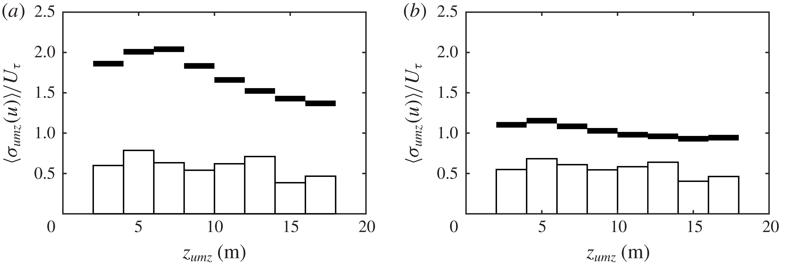
5.3 UMZ length
The distribution of the total streamwise length for the tracked UMZs is shown in figure 12(a,b). The distribution follows a power law relationship as shown by the fit in figure 12(b). Single occurrences shown as transparent markers were excluded from the fit. The longest tracked event,
 $L_{umz}=160$
m, is of the order of
 $\unicode[STIX]{x1D6FF}$
. This extent is consistent with the longest UMZs tracked by Laskari et al. (Reference Laskari, de Kat, Hearst and Ganapathisubramani2018) and approaches the range of very-large-scale motions (VLSMs) identified using turbulence spectra in the logarithmic layer (see e.g. Nickels et al.
Reference Nickels, Marusic, Hafez and Chong2005; Guala et al.
Reference Guala, Hommema and Adrian2006; Balakuma & Adrian Reference Balakuma and Adrian2007; Smits et al.
Reference Smits, McKeon and Marusic2011). Hutchins & Marusic (Reference Hutchins and Marusic2007) identified longer, meandering superstructures over 20
 $\unicode[STIX]{x1D6FF}$
in length using a spanwise array of point measurements. Consistent with Laskari et al. (Reference Laskari, de Kat, Hearst and Ganapathisubramani2018), we note the possibility that our tracked UMZs may be part of larger structures: if a tracked UMZ were to meander, the UMZ could be lost, then reappear as a new UMZ due to our lack of spanwise measurements.
Statistics of the UMZ streamwise extent
 $L_{umz}=U_{umz}T_{umz}$
. (a) The histogram of the total extent. (b) The same histogram distribution in log–log scale with a power law fit to the data. Transparent markers indicate single occurrences which were excluded from the fit. (c) The profile of the height-dependent extent
 $L_{umz}(z)$
with every third data point shown for clarity. Transparent markers indicate points within the roughness sublayer, delimited by the vertical dotted line. See figure 9(d) for definitions of
 $T_{umz}$
and
 $L_{umz}(z)$
.

The discussed limitations in defining the UMZ length, namely the underestimated duration of emerging zones and the inability to follow meandering structures, preclude a quantitative analysis of the largest UMZs. Additionally, while there may be a link between the longest zones and VLSMs, UMZs with length
 $L_{umz}\gtrsim \unicode[STIX]{x1D6FF}$
are rare and represent 0.5 % of the tracked zones. The majority of tracked UMZs have length
 $L_{umz}\lesssim 0.1\unicode[STIX]{x1D6FF}$
. The maximum size of UMZs may be bounded by
 $\unicode[STIX]{x1D6FF}$
scaling, but the average UMZ does not appear to be influenced by
 $\unicode[STIX]{x1D6FF}$
.
A profile of the height-dependent average UMZ length
 $L_{umz}(z)$
is shown in figure 12(c).
 $L_{umz}(z)$
is determined from the contributions of each zone at a given height such as the example in figure 9(d). The profile exhibits a wall-normal dependence up to approximately 11 m, above which the zone length is relatively constant. The increase of UMZ length with height is in agreement with theory for the logarithmic layer and is explored further in § 7.1. The behaviour above 11 m is discussed in § 7.4. The errors bars in figure 12(c) correspond to the aforementioned sensitivity analysis based on changing
 ${\mathcal{L}}_{x}$
by a factor of two. Importantly, varying
 ${\mathcal{L}}_{x}$
affects neither the wall-normal dependence nor the conclusions drawn from the trends. Changes in
 $L_{umz}(z)$
due to the choice of
 ${\mathcal{L}}_{x}$
were approximately uniform across all heights.
6 Vortices and the UMZ interfaces
6.1 Proximity of vortices to interfaces
In addition to the internal properties of UMZs, another important aspect of momentum zones is the interface between zones. Previous studies have shown the interfaces to carry a large portion of the instantaneous shear (see e.g. Chini et al. Reference Chini, Montemuro, White and Klewicki2017; de Silva et al. Reference de Silva, Philip, Hutchins and Marusic2017), which is consistent with the visual evidence from our data in figure 10(c,d). Large jumps in streamwise velocity occur across the interfaces, with the realization of numerous interfaces leading to the mean velocity profile (de Silva et al. Reference de Silva, Philip, Hutchins and Marusic2017).
The alignment of the UMZ interfaces with the instantaneous shear leads to the treatment of the interfaces as internal shear layers. Figures 6(b) and 10(e,f) suggest prograde vortices populate the interface shear layers. To explore the relationship of prograde vortices and the UMZ interfaces, we treat strong and persistent swirl events as vortices and track the vortex properties in time and space. See appendix A for a detailed description of the vortex identification and tracking. Outputs of the tracking include the vortex centroid position in space (
 $x_{\unicode[STIX]{x1D714}}$
,
 $z_{\unicode[STIX]{x1D714}}$
) and time (
 $t_{\unicode[STIX]{x1D714}}$
) and the equivalent radius
 $R_{\unicode[STIX]{x1D714}}$
of each vortex. Because the tracked UMZ edges are at a single streamwise location
 $x$
, the vortex centroid values were narrowed to include only the centroid height
 $z_{\unicode[STIX]{x1D714}}$
and time
 $t_{\unicode[STIX]{x1D714}}$
when the vortex crossed the
 $x$
position of the UMZ edges, yielding approximately 800 events. We then calculated the shortest path distance from each vortex centroid to the nearest tracked UMZ edge in the streamwise–wall-normal plane. We refer to this distance as the proximity
 $\unicode[STIX]{x1D6FF}_{\unicode[STIX]{x1D714}}$
. The local mean velocity
 $U(z=z_{\unicode[STIX]{x1D714}})$
was used with Taylor’s hypothesis to convert the time difference to streamwise distance. An example of the vortex proximity is shown in figure 13(a).
The proximity of tracked vortices to tracked UMZ interfaces. (a) An example of UMZ edges (black lines), prograde vortex centroids (blue dots) and vortex areas based on the equivalent radii (blue circles). The vortex proximity
 $\unicode[STIX]{x1D6FF}_{\unicode[STIX]{x1D714}}$
is the distance from the centroid to the nearest UMZ interface. (b) Binned averages of the prograde vortex equivalent diameter
 $\langle D_{\unicode[STIX]{x1D714}}\rangle$
based on the vortex centroid height
 $z_{\unicode[STIX]{x1D714}}$
with
 $\pm 20\,\%$
uncertainty bounds. (c,d) Cumulative distributions of
 $\unicode[STIX]{x1D6FF}_{\unicode[STIX]{x1D714}}$
for prograde (○) and retrograde (
 $\times$
) vortices normalized by the equivalent radius
 $R_{\unicode[STIX]{x1D714}}$
and the average UMZ thickness
 $\langle H_{umz}\rangle$
, respectively.

The cumulative distribution function (cdf) of
 $\unicode[STIX]{x1D6FF}_{\unicode[STIX]{x1D714}}$
in figure 13(c,d) normalizes the proximity by the vortex equivalent radius
 $R_{\unicode[STIX]{x1D714}}$
and average UMZ thickness
 $\langle H_{umz}\rangle$
, respectively. More than 60 % of prograde vortices are within their own radius of the nearest UMZ edge such that a majority of tracked vortices overlap a tracked UMZ interface.
 $\unicode[STIX]{x1D6FF}_{\unicode[STIX]{x1D714}}$
is also small relative to the zone thickness, with more than 60 % of vortices within 0.1
 $H_{umz}$
of the nearest interface. Note that outliers such as the vortex at the bottom of figure 13(a) are in part due to the inability of our tracking procedure to detect UMZ interfaces along the bottom of the field, leading to long distribution tails (5 % occurrence of
 $\unicode[STIX]{x1D6FF}_{\unicode[STIX]{x1D714}}>5R_{\unicode[STIX]{x1D714}}$
).
In contrast, the proximity of retrograde vortices is uniformly distributed, as indicated by the linear trends in each cdf. The lack of an observed relationship between the locations of the retrograde vortices and shear interfaces shows that the proximity of prograde vortices is a robust result and not an artefact of the methodology. Therefore, in addition to the UMZ interfaces carrying a majority of the instantaneous shear (de Silva et al. Reference de Silva, Philip, Hutchins and Marusic2017), we show the strong prograde vortices to primarily reside along these internal shear layers. While this result is unsurprising, we are not aware of any previous studies providing statistical evidence such as in figure 13.
The average prograde vortex diameter, shown in figure 13(b), appears to be independent of wall-normal distance within our field of view. Note that we might have seen a weak dependence if the range of wall-normal distance were more extensive in
 $\unicode[STIX]{x1D6FF}$
. Herpin et al. (Reference Herpin, Stanislas, Foucaut and Coudert2013) observed the spanwise vortex size to slowly increase with wall-normal distance throughout the boundary layer. De Silva et al. (Reference de Silva, Philip, Hutchins and Marusic2017) similarly found the shear interface thickness to vary weakly with wall-normal distance. The overall average diameter of tracked prograde vortices is
 $\langle D_{\unicode[STIX]{x1D714}}\rangle =$
 $0.78\pm 0.16$
m. In the following section we compare the vortex size with the UMZ interface thickness.
6.2 Interface properties
To evaluate statistical properties of the interfaces, we follow the same conditional averaging procedure as de Silva et al. (Reference de Silva, Philip, Hutchins and Marusic2017) and treat the interface as a shear mixing layer. For each UMZ edge point, the reference frame is adjusted relative to the interface height
 $z_{i}$
and statistics are compiled as functions of the wall-normal distance from the interface, i.e.
 $z-z_{i}$
and
 $\langle U-U_{i}\rangle$
. Figure 14(a) shows an example velocity contour with the UMZ interface vector coordinates (blue dots) and the neighbouring coordinates (black dots) used to represent the interface reference frame. The interfaces were conditionally sampled before computing the averaged velocity profiles. To avoid offsetting effects, interfaces with high-speed UMZs below low-speed UMZs, e.g. the interfaces at
 $z_{i}\approx$
10 m for frames 4 and 5 in figure 14(a), were excluded from the averaging. These interfaces represented 14 % of all interfaces. Instantaneous interface profiles were also excluded if there was another UMZ interface within 5
 $\unicode[STIX]{x0394}z$
in the same frame. 20 % of the remaining profiles were excluded based on this condition such that 69 % of the overall interfaces were used for the analysis. Figure 14(b) shows the resulting conditionally averaged streamwise velocity profile relative to the interfaces.
Demonstration of the UMZ interface conditional profile following figure 7 of de Silva et al. (Reference de Silva, Philip, Hutchins and Marusic2017). (a) A streamwise velocity colour plot sample with tracked UMZ edges (blue lines), vector field coordinates at
 $z_{i}$
interfaces (blue dots) and coordinates surrounding the interfaces (black dots). (b) The streamwise velocity profile in the frame relative to the interface height
 $z_{i}$
, averaged for all edges. The profile indicates the maximum shear
 $\unicode[STIX]{x2202}\langle U\rangle /\unicode[STIX]{x2202}z|_{max}$
(red line) and average streamwise velocity jump
 $\unicode[STIX]{x0394}U_{i}$
(thick black line) used to calculate the interface thickness
 $\unicode[STIX]{x1D6FF}_{i}=0.85\pm 0.04$
m. (c) The average streamwise velocity jump
 $\unicode[STIX]{x0394}U_{i}$
normalized by
 $U_{\unicode[STIX]{x1D70F}}$
, following figure 13(a) of de Silva et al. (Reference de Silva, Philip, Hutchins and Marusic2017). Closed squares in (c) correspond to de Silva et al. (Reference de Silva, Philip, Hutchins and Marusic2017) and open circles correspond to the current study.

The value of
 $\unicode[STIX]{x0394}U_{i}$
, shown as a black line in figure 14(b), describes the streamwise velocity jump across the interface. Figure 14(c) compares the normalized value of
 $\unicode[STIX]{x0394}U_{i}$
from our data with the experimental results of de Silva et al. (Reference de Silva, Philip, Hutchins and Marusic2017). To normalize our velocities, we use the
 $U_{\unicode[STIX]{x1D70F}}$
value from table 2 and a nominal estimate
 $U_{\infty }=6.6~\text{m}~\text{s}^{-1}$
which is the mean velocity at the top of the met tower. The momentum deficit corresponds to a wall-normal position
 $z$
approximately in the centre of our FOV, and the vertical error bars represent the estimated momentum deficits at the FOV limits. The strong agreement for
 $\unicode[STIX]{x0394}U_{i}^{+}$
confirms the velocity jump across the shear interfaces is
 $\unicode[STIX]{x0394}U_{i}\sim O(U_{\unicode[STIX]{x1D70F}})$
as suggested by de Silva et al. (Reference de Silva, Philip, Hutchins and Marusic2017). Binning our interfaces based on wall-normal distance revealed
 $\unicode[STIX]{x0394}U_{i}$
to decrease slowly with increasing wall-normal distance. However, the convergence of
 $\unicode[STIX]{x0394}U_{i}(z)$
statistics was not satisfactory and we show
 $\unicode[STIX]{x0394}U_{i}$
averaged at a single representative point in figure 14(c). The possible wall-normal trend (not shown) agrees with the findings of de Silva et al. (Reference de Silva, Philip, Hutchins and Marusic2017) that
 $\unicode[STIX]{x0394}U_{i}$
decreases with decreasing momentum deficit (or increasing wall-normal distance), but remains within the range
 $\unicode[STIX]{x0394}U_{i}=U_{\unicode[STIX]{x1D70F}}-2U_{\unicode[STIX]{x1D70F}}$
.
Following Brown & Roshko (Reference Brown and Roshko1974) and de Silva et al. (Reference de Silva, Philip, Hutchins and Marusic2017), we calculated the thickness of the UMZ interface
 $\unicode[STIX]{x1D6FF}_{i}$
as
 $$\begin{eqnarray}\unicode[STIX]{x1D6FF}_{i}=\frac{\unicode[STIX]{x0394}U_{i}}{\unicode[STIX]{x2202}\langle U\rangle /\unicode[STIX]{x2202}z|_{max}},\end{eqnarray}$$
where
 $\unicode[STIX]{x2202}\langle U\rangle /\unicode[STIX]{x2202}z|_{max}$
is the maximum shear. Each element of (6.1) is demonstrated in figure 14(b), including the average interface thickness
 $\unicode[STIX]{x1D6FF}_{i}=0.85\pm 0.04$
m. The uncertainty bounds are based on confidence intervals of the fits used to determine
 $\unicode[STIX]{x0394}U_{i}$
.
The average interface thickness calculated above is based on UMZ interfaces across the entire range of
 $z$
in the field of view. Separating the interfaces based on their height does not significantly change the resulting thickness. The average thickness for interfaces within the roughness sublayer (
 $z_{i}<5.5$
m) is
 $\unicode[STIX]{x1D6FF}_{i}=0.81\pm 0.06$
m and for interfaces above the roughness sublayer is
 $\unicode[STIX]{x1D6FF}_{i}=0.83\pm 0.05$
m. The difference between the two is within the uncertainty bounds.
The average interface thickness
 $\unicode[STIX]{x1D6FF}_{i}$
is only 9 % larger than the average prograde vortex diameter
 $\langle D_{\unicode[STIX]{x1D714}}\rangle$
, despite using two unrelated methods. The 9 % difference is within the uncertainty bounds of
 $\langle D_{\unicode[STIX]{x1D714}}\rangle$
. Based on the agreement between
 $\unicode[STIX]{x1D6FF}_{i}$
and
 $D_{\unicode[STIX]{x1D714}}$
, prograde vortices statistically extend across the shear layer separating momentum zones. We stress that the results for
 $\langle D_{\unicode[STIX]{x1D714}}\rangle$
and
 $\unicode[STIX]{x1D6FF}_{i}$
are limited by the coarse spatial resolution relative to the vortex diameter and interface thickness: the SLPIV vector spacing
 $\unicode[STIX]{x0394}x=0.27$
m is only three times
 $\langle D_{\unicode[STIX]{x1D714}}\rangle$
and
 $\unicode[STIX]{x1D6FF}_{i}$
. The effect of spatial resolution is not accounted for in the above uncertainty bounds. We therefore treat the average values as the characteristic sizes of the large vortices and interfaces whose size can be resolved in our measurements.
7 Discussion: the dynamic role of UMZs and the internal shear layers
We have provided evidence showing the structure of the logarithmic region in the fully rough, very-high-
 $Re$
ASL to be qualitatively similar to the structure of wall-bounded turbulent flows at the laboratory scale. Consistent with laboratory-scale studies, our flow field is populated by thin regions of strong local shear and vorticity separating relatively larger regions of uniform momentum (Meinhart & Adrian Reference Meinhart and Adrian1995; Priyadarshana et al.
Reference Priyadarshana, Klewicki, Treat and Foss2007; de Silva et al.
Reference de Silva, Hutchins and Marusic2016). Instantaneous realizations of these internal shear layers show their relation to the signature of hairpin packets and to the inclination of ramp-like structures. In this section, we use the properties of the UMZs and shear interfaces to explore further their relation to existing theory and their contribution to overall boundary layer dynamics.
7.1 Results in the context of the attached eddy hypothesis (AEH)
The basis of the AEH of Townsend (Reference Townsend1976) is that the presence of the wall directly influences the main turbulent motions in the inertial logarithmic region. The motions, considered to be eddies, scale directly in size and inversely in population density with wall-normal distance. The velocity of the eddies scales with
 $U_{\unicode[STIX]{x1D70F}}$
. Populating the flow with a random superposition of these eddies leads to the Reynolds stress profiles, specifically the equations given in § 3.2.2 and the invariance of the Reynolds shear stress
 $-\overline{uw}^{+}$
. The size and velocity scaling of the eddies is also consistent with the mixing length model of Prandtl (Reference Prandtl1925) and arguments leading to (3.2). See Perry & Marusic (Reference Perry and Marusic1995) or Nickels et al. (Reference Nickels, Marusic, Hafez, Hutchins and Chong2007) for a more detailed summary of the AEH.
An important consideration for the AEH is defining the representative eddy. In attached eddy models, the choice of the representative eddy dictates how well the model can reproduce statistical features of the flow. The representative eddy must also relate to observations from numerical and experimental studies. Treating streamwise-correlated hairpin packets as the representative eddy in the AEM works well in both these regards (Marusic Reference Marusic2001). We use our extensive log region to relate our results to the AEH and to compare our findings with the interpretation of the hairpin packet as the representative eddy.
Figure 15 provides the number density and size of tracked UMZs and tracked vortices as a function of wall-normal distance
 $z$
. The number density
 $N$
in figure 15(a) is the number of unique tracked zones or vortices occurring at each height and is analogous to a pdf of
 $z_{umz}$
or
 $z_{\unicode[STIX]{x1D714}}$
, respectively. The number density exhibits a near-linear decrease with increasing
 $z$
for both UMZs and vortices in the region between the dotted lines. We therefore infer this region,
 $z=5.5$
–11 m, to be the canonical logarithmic region. While the logarithmic region extends up to approximately
 $z=70$
m, the turbulent behaviour above
 $z=11$
m is non-canonical. We discuss the distinction between the canonical and non-canonical portions of the logarithmic region in § 7.4.
Assuming each UMZ is separated in the streamwise direction by a shear interface where the vortices primarily reside, the number density of UMZs and vortices should be similar. This is confirmed by the agreement in the canonical region of the two distributions in figure 15(a) which result from independent tracking methodologies. The linear decrease in number density of spanwise vortices is in agreement with the findings of Wu & Christensen (Reference Wu and Christensen2006) and Herpin et al. (Reference Herpin, Stanislas, Foucaut and Coudert2013).
Comparison of UMZ (○) and vortex (●) properties as a function of wall-normal distance: (a) the number density
 $N$
and (b) the characteristic UMZ length
 $L_{umz}$
, vortex size
 $D_{\unicode[STIX]{x1D714}}$
and mixing length
 $l=\unicode[STIX]{x1D705}z$
(line). The dotted lines correspond to the approximate limits of the region exhibiting canonical behaviour. Error bars for
 $D_{\unicode[STIX]{x1D714}}$
are included, but do not exceed the marker size.

The characteristic lengths of UMZs and vortices, provided in previous figures, are shown together in figure 15(b). Whereas the vortex size
 $D_{\unicode[STIX]{x1D714}}$
appears relatively independent of the wall-normal distance, the UMZ length
 $L_{umz}$
increases with
 $z$
. Given the combined presence of UMZs and shear interfaces with vortices in the structure of the boundary layer, we expect a potential characteristic length scale to be between
 $L_{umz}(z)$
and
 $D_{\unicode[STIX]{x1D714}}$
. Figure 15(b) shows the mixing length
 $l=\unicode[STIX]{x1D705}z$
to fall between the two scales in agreement with this expectation.
To further demonstrate the dynamic role of UMZs, we used the tracked UMZ properties to assess their effect on the streamwise mean and r.m.s. profiles. Reproducing flow statistics based on UMZs and their interfaces has been shown to work well (Chini et al.
Reference Chini, Montemuro, White and Klewicki2017; de Silva et al.
Reference de Silva, Philip, Hutchins and Marusic2017). For our spatio-temporal (
 $z,t$
) SLPIV signal, we created an artificial signal by assigning each vector index the average modal velocity
 $U_{umz}$
of the UMZ to which the vector belongs. The resulting signal, the stepwise function shown in figure 16(a), contains no information relating to the shear interfaces except for the velocity jump
 $\unicode[STIX]{x0394}U_{i}$
between zones. The UMZ signal works similarly to a low-pass filter such that large-scale trends equal to and greater than the UMZ duration are captured. The mean profile of the UMZ signal in figure 16(b) matches closely with the SLPIV profile, except for the bottom and top of the image field where the tracking methodology is biased as previously discussed. The streamwise turbulence in figure 16(c) is fairly well represented, though the energy is overestimated by the UMZ signal at lower heights (due to excluding the relatively smoother transitions across the zone interfaces) and underestimated at higher
 $z$
values (due to excluding fluctuations within zones).
A comparison of the SLPIV signal (circles) with an artificial velocity signal based on UMZ modal velocities (lines). (a) A 5-second sample time signal at
 $z=10$
m. (b) The streamwise mean velocity profile. (c) The streamwise r.m.s. velocity profile. The dotted lines correspond to the limits as in figure 15.

Qualitatively, figure 16(c) demonstrates that the UMZs, along with larger-scale motions, govern the variance in the streamwise velocity. The variance profile, realized in the passing of successive UMZs, confirms the importance of the UMZ passing frequency (which scales with
 $z$
, consistent with the length and number density) and the velocity jump between zones (which scales with
 $U_{\unicode[STIX]{x1D70F}}$
). The UMZs represent the energy-containing eddies in that they are responsible for a majority of the streamwise variance. This suggests
 $\unicode[STIX]{x0394}U_{i}$
and
 $L_{umz}$
as the relevant scales for the energy transfer rate of the energy-containing eddies
 $\unicode[STIX]{x1D716}\sim u_{o}^{3}/l_{o}$
. Because the velocity jump is approximately equal to the streamwise r.m.s. velocity
 $\unicode[STIX]{x1D70E}_{u}$
for our data, we can approximate the dissipation as
 $\unicode[STIX]{x1D716}\sim \unicode[STIX]{x1D70E}_{u}^{3}/L_{umz}$
.
With regard to the AEH, we interpret figures 15 and 16 as follows: UMZs have features consistent with the AEH, namely the wall-normal trends of number density and size postulated in the AEH. Further, the velocity and length scales of the UMZs lead to both the mean velocity and streamwise variance profiles. The UMZs are therefore a key feature of the boundary layer structure. However, the UMZs lack the strain and vorticity dynamics necessary to influence the flow around it and generate new structures. The UMZ properties are likely a manifestation of dynamics within the internal shear layers separating UMZs. The internal shear layers with embedded vortices have been proposed as an archetypal flow structure (Elsinga & Marusic Reference Elsinga and Marusic2010; Ishihara et al. Reference Ishihara, Kaneda and Hunt2013; Wei et al. Reference Wei, Elsinga, Brethouwer, Schlatter and Johansson2014). The size of UMZs may then be the direct result of the number density and distribution of the shear layers separating the zones. To capture both the flow statistics and dynamics, the representative eddy must include both the internal shear layer and the corresponding region of uniform momentum between the adjacent shear layers. Additionally, based on the shape of the two-point correlation, the average internal shear layer must have a forward inclination.
Our experimental support for the internal shear layer and corresponding UMZ as the representative eddy is compatible with the basic framework of the hairpin vortex packet used in the AEM (e.g. the
 $\unicode[STIX]{x1D6EC}$
packet-eddy). In both cases, the shear layer has a forward inclination, is embedded with vortices, and has an associated UMZ. De Silva et al. (Reference de Silva, Hutchins and Marusic2016), using an opposite approach, showed that a synthetic velocity field created from
 $\unicode[STIX]{x1D6EC}$
packet eddies could reproduce the UMZ properties measured by their experiments. Together with the AEM results of de Silva et al. (Reference de Silva, Hutchins and Marusic2016), our experimental findings demonstrate the close relationship between the observed zonal structure of the boundary layer and the concept of attached eddies.
7.2 The mean shear and large-scale anisotropy
If the UMZ modal velocities lead to the mean velocity profile as in figure 16(b), the UMZs must also lead to the mean velocity gradient
 $S=\unicode[STIX]{x2202}U/\unicode[STIX]{x2202}z$
. Given uniform streamwise velocities within each zone, the mean shear must predominantly result from the internal shear layers which are separated by the UMZ thickness
 $H_{umz}$
. The mean shear is therefore likely to scale as
 $S\sim \unicode[STIX]{x0394}U_{i}/H_{umz}$
. In the log region, the shear is defined as
 $S=U_{\unicode[STIX]{x1D70F}}/\unicode[STIX]{x1D705}z$
. Having already shown
 $\unicode[STIX]{x0394}U_{i}\sim O(U_{\unicode[STIX]{x1D70F}})$
where
 $\unicode[STIX]{x0394}U_{i}$
varies weakly with
 $z$
(de Silva et al.
Reference de Silva, Philip, Hutchins and Marusic2017), we require
 $H_{umz}\sim O(z)$
to satisfy the log region gradient.
Results for the height dependence of
 $H_{umz}$
are less robust than
 $L_{umz}$
because the thickness is along the same direction as
 $z$
and the edges of the field of view skew the statistics. We estimate
 $H_{umz}(z)$
using the mid-height
 $z_{umz}$
of each zone and calculating binned averages (as in figure 11) of the thickness weighted by the zone length. The resulting profile is reliable only in the centre 25 % of the field due to apparent edge effects. Figure 17 compares the mean shear
 $S$
(circles) with the UMZ approximation
 $\unicode[STIX]{x0394}U_{i}/H_{umz}(z_{umz})$
(line). The approximation in the centre of the field (black line) matches closely with the mean shear and supports the argument
 $S\sim \unicode[STIX]{x0394}U_{i}/H_{umz}$
.
The mean shear profile
 $S=\unicode[STIX]{x2202}U/\unicode[STIX]{x2202}z$
(circles) compared with the scaling argument
 $S=\unicode[STIX]{x0394}U_{i}/\langle H_{umz}\rangle (z_{umz})$
(line). Grey segments of the line correspond to regions where
 $H_{umz}(z_{umz})$
statistics are likely unreliable. The dotted lines correspond to the limits as in figure 15.
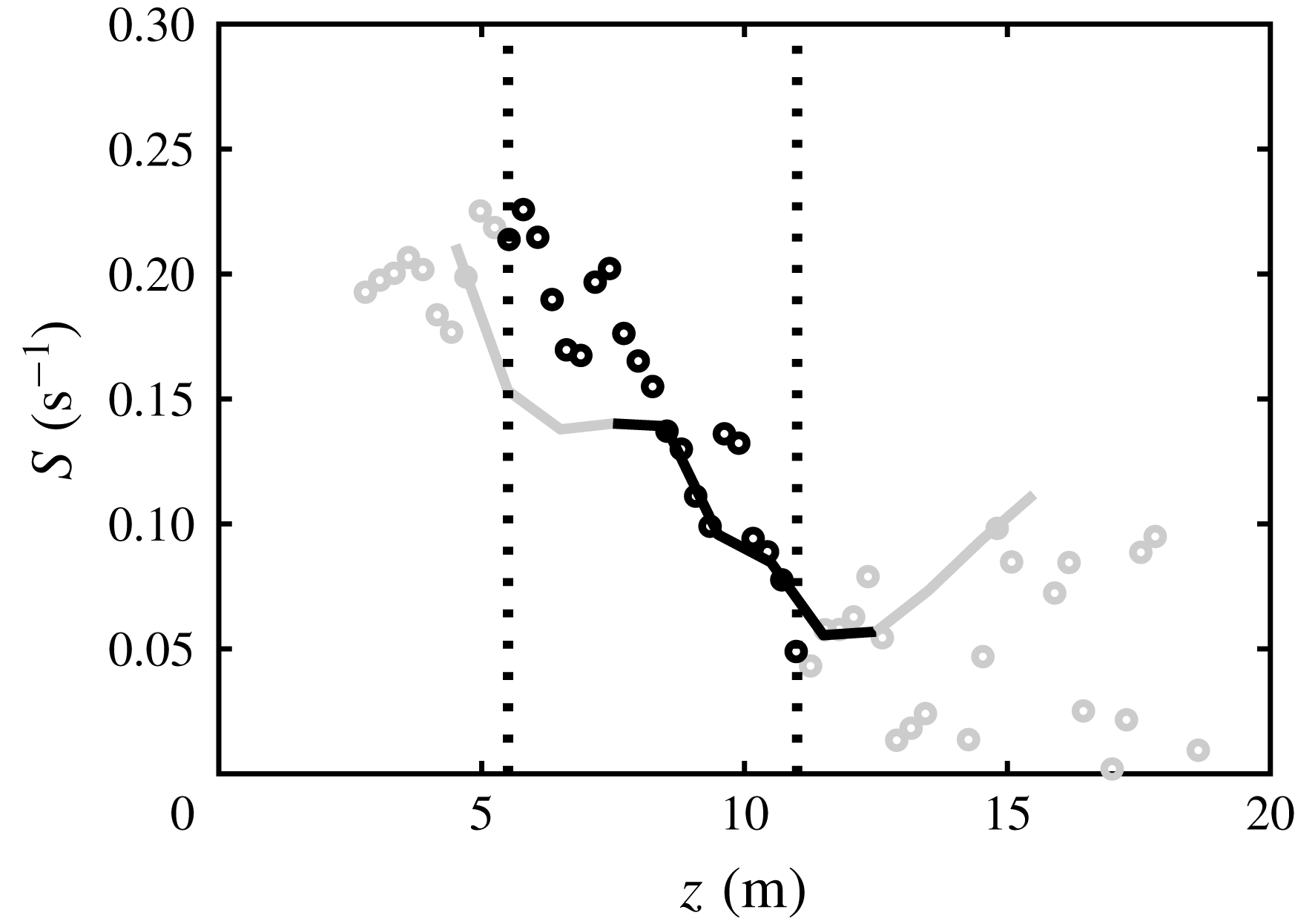
One function of the mean shear worth exploring further is its role in large-scale anisotropy. Corrsin (Reference Corrsin1958) postulated that local isotropy can occur only for turbulent scales faster than the characteristic mean strain time
 $S^{-1}$
. The scales faster than
 $S^{-1}$
correspond to the longitudinal wavenumber region
 $k_{1}\gg (S^{3}/\unicode[STIX]{x1D716})^{1/2}$
(Corrsin Reference Corrsin1958). This criterion was quantified through experiments by Saddoughi & Veeravalli (Reference Saddoughi and Veeravalli1994) as
 $k_{1}(\unicode[STIX]{x1D716}/S^{3})^{1/2}>3$
. Using the log region definitions
 $\unicode[STIX]{x1D716}\sim U_{\unicode[STIX]{x1D70F}}^{3}/\unicode[STIX]{x1D705}z$
and
 $S=U_{\unicode[STIX]{x1D70F}}/\unicode[STIX]{x1D705}z$
, the condition can be rewritten as
 $k_{1}\unicode[STIX]{x1D705}z>3$
. Alternatively, we can relate the wavenumber directly to the UMZ length as
 $k_{1}L_{umz}>O(1)$
.
To evaluate this relation, we estimated one-dimensional velocity spectra
 $\unicode[STIX]{x1D6F7}(k_{1})$
for the three velocity components of the sonic anemometer at
 $z=10$
m. The spectra were estimated using overlapping windows of 5 min for a 35-min period. The selected period, from 00:15 to 00:50 in figure 2, is statistically stationary and includes SLPIV data set 1. The results were converted from the frequency to the wavenumber domain using Taylor’s hypothesis and were smoothed to reduce white noise. Figure 18 shows the estimated spectra for the three velocity components as well as their ratios. The spectra indicate anisotropy at scales larger than the UMZ length, and local isotropy at smaller scales until the sonic anemometer high-wavenumber noise region
 $k_{1}L_{umz}>5$
. We use the term ‘local isotropy’ here to indicate equal turbulent energy density in each direction at the given scale, noting that other statistics may indicate small-scale anisotropy (Shen & Warhaft Reference Shen and Warhaft2000; Carter & Coletti Reference Carter and Coletti2017). The spectra suggest the characteristic UMZ size is an appropriate threshold for large-scale anisotropy in wall-bounded flows. This result is consistent with
 $u$
and
 $w$
deviations within the zones being approximately equal (see figure 11). The spectra also show that the identified UMZs are not the largest scales of the flow.
 $L_{umz}$
appears to be well within the inertial subrange of the streamwise spectrum, and thus in the wavenumber region where self-organization is expected.
The one-dimensional velocity spectrum
 $\unicode[STIX]{x1D6F7}$
as a function of longitudinal wavenumber
 $k_{1}$
estimated using sonic anemometer measurements at
 $z=10$
m with 5-min windows. (a) The smoothed dimensional spectra with the wavenumbers corresponding to the average UMZ length
 $L_{umz}(z=10~\text{m})$
and vortex diameter
 $D_{\unicode[STIX]{x1D714}}$
indicated for reference, and an example unsmoothed spectrum included for
 $\unicode[STIX]{x1D6F7}_{u}$
(grey line). (b–d) The ratios of spectra with
 $k_{1}$
normalized by
 $L_{umz}$
, where a ratio of 1 indicates statistical isotropy.

Following Corrsin (Reference Corrsin1958), wall-bounded shear flows can be separated into two turbulent scale regions: large scales which interact directly with the mean shear and production (
 $k_{1}z\gtrsim O(1)$
) and smaller scales which do not (the cascade; Jiménez Reference Jiménez2018). By showing the mean shear profile and large-scale anisotropy to be closely related to the UMZ properties, we demonstrate that the internal shear layers and associated uniform regions (i.e. the zonal structure of the boundary layer) interact directly with the mean shear and contribute to the production of turbulence.
7.3 A note of caution regarding the interpretation of UMZs
For this work, we have adopted the uniform momentum zone terminology of Meinhart & Adrian (Reference Meinhart and Adrian1995) due to use of the same experimental set-up, i.e. streamwise–wall-normal PIV, and histogram methodology to identify zones. We stress that the UMZ terminology describes a relative quality: the identified regions have uniform streamwise velocity relative to all the velocities in the experimental field of view represented by the histogram. The identified UMZs in a given frame are therefore dependent on the histogram field of view and spatial resolution in addition to the flow itself. In a hypothetical study for which the spatial resolution is not the limiting factor, the key parameter is the previously discussed streamwise extent
 ${\mathcal{L}}_{x}$
of the histogram field.
 ${\mathcal{L}}_{x}$
can theoretically be reduced to
 $O(\unicode[STIX]{x1D702})$
to identify the sub-Kolmogorov scales as uniform regions. However, the UMZ analysis is more useful for studying dynamics in the range of large-scale anisotropy where relatively uniform regions separate the internal shear layers. The approximate wavenumber limit for large-scale anisotropy scales with wall-normal distance as
 $k_{1}z\sim O(1)$
(Saddoughi & Veeravalli Reference Saddoughi and Veeravalli1994; Jiménez Reference Jiménez2018). The UMZs identified in our analysis have the same wall-normal scaling behaviour
 $L_{umz}\sim z$
and the average UMZ length corresponds to the limit of large-scale anisotropy inferred from the turbulence spectra in figure 18. We conclude that, for studies including the logarithmic layer, the streamwise extent should meet the condition
 ${\mathcal{L}}_{x}/L_{umz}\sim {\mathcal{L}}_{x}/z_{min}<1$
in order to identify the relevant UMZs.
 $z_{min}$
represents the minimum height in the region of interest. Additionally,
 ${\mathcal{L}}_{x}$
should be larger than the internal shear layers
 $\unicode[STIX]{x1D6FF}_{i}$
. For our analysis, the normalized extent is
 ${\mathcal{L}}_{x}/\unicode[STIX]{x1D6FF}_{i}\approx 2$
and
 ${\mathcal{L}}_{x}/z_{min}\approx 0.3$
, where the minimum height is
 $z_{min}=5.5$
m. Our selected frame span is therefore long enough to not identify the advection velocity of each vortex and shear interface as a histogram peak and short enough to capture the regions responsible for large-scale anisotropy.
The UMZs identified in previous works such as de Silva et al. (Reference de Silva, Hutchins and Marusic2016) and in our study both exhibit step-like instantaneous profiles, but the size characteristics cannot be compared quantitatively due to differences in
 ${\mathcal{L}}_{x}$
and the inclusion of temporal tracking. In light of how UMZs are defined and the sensitivity of results to
 ${\mathcal{L}}_{x}$
, we focus our interpretation of UMZ results to qualitative features such as the scaling relationships and wall-normal trends apparent in figure 15. Further, our UMZ analysis lacks spanwise measurements to characterize the three-dimensional characteristics of the uniform regions in our flow field. The regions of coherence we experimentally identify as UMZs may be associated with different types of coherent structures previously classified in the literature. In instances of inclined shear layer events such as in figure 6, the two UMZs resemble Reynolds stress events with uniform
 $uw$
(Jiménez Reference Jiménez2018), referred to as sweep and ejection events (Adrian et al.
Reference Adrian, Meinhart and Tomkins2000b
) or superbursts (Na, Hanratty & Liu Reference Na, Hanratty and Liu2001). The UMZs are also qualitatively similar to the wake region between vortex clusters (del Álamo et al.
Reference del Álamo, Jiménez, Zandonade and Moser2006) and streamwise velocity streaks (Jiménez Reference Jiménez2018).
7.4 Deviation from the canonical boundary layer
The results presented thus far are consistent with smooth wall observations at lower
 $Re_{\unicode[STIX]{x1D70F}}$
in laboratory settings. However, discrepancies emerge in the upper portion of the SLPIV field. We have presented certain inconsistencies in the results, e.g. a decline in the Reynolds shear stress in figure 5 and the flattening of the inclined structures in figure 7. In particular, the UMZ number density and size trends in figure 15 show a departure from log layer theory around
 $z=11$
m. The figure 19 profile of the two-point correlation inclination angle
 $\unicode[STIX]{x1D6FE}$
is consistent with this departure.
 $\unicode[STIX]{x1D6FE}$
decreases below the traditional
 $10^{\circ }$
to
 $15^{\circ }$
range at
 $z=11$
m. Above
 $z=11$
m, there are fewer vortices present as seen in figure 15(a). Correspondingly, there are fewer shear layers to separate momentum zones. The UMZs occupy a majority of the field above
 $z=11$
m, leading to a constant length
 $L_{umz}$
. With longer zones and fewer shear interfaces, the structures become statistically flatter and the two-point correlation inclination angle decreases as shown in figure 19. As a result of the decrease in shear interfaces and vortices, turbulence properties such as the Reynolds shear stress exhibit marked decreases.
The profile of the two-point correlation inclination angle
 $\unicode[STIX]{x1D6FE}$
. The dotted lines correspond to the limits of the region exhibiting canonical log layer behaviour. Every third point is shown for clarity.

One explanation for the decrease in turbulence is thermal stability. Despite a very shallow temperature gradient
 $\unicode[STIX]{x2202}\unicode[STIX]{x1D703}_{v}/\unicode[STIX]{x2202}z$
, i.e. less than
 $0.5\,^{\circ }\text{C}$
per 100 m in figure 2(c), the flux Richardson number at
 $z=30$
m in table 1 indicates non-negligible thermal stability. We therefore believe the thermal stability is modulating the production of turbulence. Based on the
 $R_{f}$
values in table 1, the stability is height-dependent such that stability effects are negligible near the surface and become increasingly important above 11 m. This height is well within the surface layer, and the mean velocity continues to exhibit log–linear behaviour up to 70 m.
A second explanation, following the argument of Hunt & Carlotti (Reference Hunt and Carlotti2001), is that the surface layer is further separated into two sublayers: a near-wall region where turbulent motions interact directly with the wall (i.e. are ‘attached’) and an upper region where top-down turbulent motions are detached from the wall. The extent of the near-wall region predicted by Hunt & Carlotti (Reference Hunt and Carlotti2001) matches well with our observations.
Another possibility is that both explanations are relevant. In our case, the upper region of Hunt & Carlotti (Reference Hunt and Carlotti2001) is characterized by thermal-driven features and is stably stratified, while the near-wall region is characterized by mechanically produced turbulence and is thermally neutral. Top-down motions from the stable upper region may sporadically interact with the near-wall region. This may then lead to the stability effects within the top of our FOV, which are stronger than the local stability parameter would indicate (i.e.
 $Ri_{f}=0.05$
at
 $z=30$
m). However, the distinction between the two potentially coupled explanations is irrelevant to the specific conclusions of our work, as both interpretations include a canonical region with observed wall-attached behaviour which is the focus of our analysis.
8 Summary and conclusions
In this work we have presented new SLPIV measurements using snow particles as tracers in the atmospheric surface layer. Together with met-mounted anemometer measurements, the SLPIV measurements comprise three 15-min periods and are presented in the context of a fully rough turbulent boundary layer with
 $Re_{\unicode[STIX]{x1D70F}}\sim O(10^{6})$
. The field of view, having 60 vectors from
 $z=3$
to 19 m, provides a high-resolution streamwise–wall-normal spatial plane covering the top of the roughness sublayer and the bottom of the logarithmic region. The mean velocity profile follows a log–linear increase with height in accordance with the logarithmic region up to
 $z=$
70 m, but turbulence profiles such as the Reynolds shear stress exhibit canonical wall-normal trends in the smaller range
 $z=5.5$
to 11 m. The high spatial resolution – relative to previous field studies at SLTEST and QLOA – allows for detailed observation and analysis of spatial structures in the logarithmic region at the atmospheric scale. The current results add to the growing record of laboratory- and field-scale studies in support of Reynolds number similarity. The results also represent the first quantitative investigation of atmospheric turbulence structures using whole-field imaging.
Through visual and statistical methods, we identified hallmark features of boundary layer turbulence previously observed using PIV in lower Reynolds number flows. In particular, we observed instantaneous realizations of forward-inclined vortex structures having the same signature as hairpin vortex packets (Adrian et al.
Reference Adrian, Meinhart and Tomkins2000b
). The vortex structures separated regions of uniform streamwise and wall-normal momentum. We infer the vortex structures and uniform momentum regions (i.e. UMZs) to be collectively responsible for the inclination angle of the two-point correlation contours of the streamwise velocity fluctuations. Our two-point correlations exhibit the same
 $10^{\circ }$
to
 $15^{\circ }$
inclination angle observed in previous smooth and rough wall studies (see e.g. Christensen & Adrian Reference Christensen and Adrian2001; Volino et al.
Reference Volino, Schultz and Flack2007). These results suggest a universality of the inclined vortex structures and corresponding UMZs in the logarithmic region across a wide range of Reynolds number, regardless of surface roughness, which is in agreement with the wall similarity hypothesis of Townsend (Reference Townsend1976).
In addition to sharing the signature of hairpin packets, the vortex structures more generally align with thin regions of strong wall-normal shear known as internal shear layers. By tracking UMZs in the spatio-temporal SLPIV signal, we extended the instantaneous realizations described above and showed the atmospheric surface layer to have the same zonal structure as laboratory-scale boundary layers, where the flow spatially consists of UMZs separated by the internal shear layers (de Silva et al.
Reference de Silva, Hutchins and Marusic2016). Through statistical evidence, the prograde vortices were observed to concentrate in the proximity of these shear interfaces and have the same characteristic size as the interface thickness. The velocity scale of the shear interfaces, i.e.
 $U_{\unicode[STIX]{x1D70F}}$
, is in agreement with de Silva et al. (Reference de Silva, Philip, Hutchins and Marusic2017).
Further analysis of the internal shear layers and UMZs revealed their contribution to the overall velocity statistics. Similar to the findings of Chini et al. (Reference Chini, Montemuro, White and Klewicki2017) and de Silva et al. (Reference de Silva, Philip, Hutchins and Marusic2017), we used a simplified representation of the zonal structure to reproduce wall-normal profiles of the mean streamwise velocity, mean shear and streamwise variance. These results have implications for the AEM and low-order modelling in general, where the overall flow field can be reasonably well captured by considering only the internal shear layers and UMZs. Wall-normal trends of the number density and characteristic size of the tracked vortices and UMZs suggest the internal shear layer (with embedded prograde vortices) and the corresponding UMZ to be a good candidate for representative eddy in the AEM. The internal shear layers and UMZs are therefore salient features of turbulent boundary layers, in terms of both the spatial composition and turbulent energy of the flow.
We acknowledge the error bars shown in various figures do not encompass all of the uncertainties and limitations present in the field experiment. Though difficult to quantify, contributing factors such as particle inertia, atmospheric effects and sensitivity to analysis methods are specifically discussed throughout the manuscript. Our findings – based primarily on qualitative wall-normal trends, scaling arguments and comparisons with existing theory – show that the structure of wall turbulence in the aerodynamically rough atmospheric surface layer is consistent with turbulent boundary layers at laboratory-scale Reynolds numbers.
Acknowledgements
The authors gratefully acknowledge A. Petersen and A. Nemes for their facilitation of PIV processing. We are also thankful to several individuals for their discussions pertaining to this work, specifically to E. Bou-Zeid regarding atmospheric effects and A. J. Smits regarding scaling. We acknowledge funding support from the Institute on the Environment (IonE). J.H. and M.G. are both supported by a National Science Foundation CAREER grant (NSF-CBET-1454259 and NSF-CBET-1351303, respectively).
Supplementary movie
A supplementary movie is available at https://doi.org/10.1017/jfm.2018.759.
Appendix A. Tracking vortex events
A.1 Methodology
This appendix describes the methodology used to track vortex events in the spatio-temporal SLPIV data. We identified vortices based on values of the swirling strength
 $\unicode[STIX]{x1D706}_{ci}$
in the vector field (see e.g. Adrian, Christensen & Liu Reference Adrian, Christensen and Liu2000a
). The sign of
 $\unicode[STIX]{x1D706}_{ci}$
was prescribed using the sign of the out-of-plane vorticity
 $\unicode[STIX]{x1D714}_{y}$
. We used
 $\unicode[STIX]{x1D706}_{thr}=0.55~\text{s}^{-1}$
as the high-pass cutoff threshold. The choice of
 $\unicode[STIX]{x1D706}_{thr}$
is discussed further in § A.2. To track events, contiguous regions above the threshold in the three-dimensional spatio-temporal domain were recorded if the region extended for at least 8 frames, i.e. 0.25 s. The temporal (frame) filter is required to exclude measurement noise which is enhanced in the derivative calculation. The combination of the cutoff threshold, temporal filtering and SLPIV spatial resolution limit the focus of the tracking procedure to relatively large, persistent vortex events. Almost 4000 vortex events in SLPIV data set 1 were identified as a result of the tracking.
For each frame in an identified event, the vortex has an area
 $A_{\unicode[STIX]{x1D714}}$
given by contours of the threshold
 $\unicode[STIX]{x1D706}_{thr}$
. The vortex centre is calculated as the geometric centroid of the area weighted by the swirling strength values. Using the vortex area, the characteristic size is determined assuming the vortex is circular. The equivalent radius of the vortex in each frame is
 $R_{\unicode[STIX]{x1D714}}=\sqrt{A_{\unicode[STIX]{x1D714}}/\unicode[STIX]{x03C0}}$
and the equivalent diameter
 $D_{\unicode[STIX]{x1D714}}$
is twice the radius. Figure 20(a) provides an example of the vortex properties for the same SLPIV frame as figure 6. The tracked vortices are characterized by their outline (i.e. contours of
 $\unicode[STIX]{x1D706}_{thr}$
, black lines), centroid position (green dots), and equivalent diameter.
The distribution of equivalent diameters is shown in figure 20(b). Based on the distribution tails, large diameter prograde vortices (
 $\unicode[STIX]{x1D706}_{ci}<0$
, aligned with the mean shear) are more likely than retrograde events. The lack of small diameter statistics (
 $D_{\unicode[STIX]{x1D714}}<0.5$
m) is due to the spatial resolution limits. If we had resolved the Kolmogorov scales, we would have identified smaller vortices and distribution modes would occur at smaller vortex diameters. Herpin et al. (Reference Herpin, Stanislas, Foucaut and Coudert2013) found the log–normal distribution to best describe the mode of the diameter distribution, but the log–normal distribution does not represent well the rare events. Our results suggest a power law is appropriate for describing the tail of the vortex diameter distribution (fit not shown).
A demonstration of the vortex event tracking methodology. (a) A swirling strength colour plot for an example frame including contours of the cutoff threshold
 $\unicode[STIX]{x1D706}_{thr}$
(black lines), tracked vortex centroids (green dots) and circular representations of the equivalent diameter
 $D_{\unicode[STIX]{x1D714}}$
(green dashed circles). (b) The histogram of the vortex equivalent diameter
 $D_{\unicode[STIX]{x1D714}}$
with separate distributions based on the rotation direction of the vortex. (c) Binned averages of the shape factor
 $\langle SF\rangle$
based on the equivalent diameter. (d)
 $\langle D_{\unicode[STIX]{x1D714}}\rangle$
as a function of
 $\unicode[STIX]{x1D706}_{thr}$
for a 2000 frame sample, where the filled data marker indicates the
 $\unicode[STIX]{x1D706}_{thr}$
value used for the full analysis and the shaded region is within
 $\pm 20\,\%$
of
 $D_{\unicode[STIX]{x1D714}}$
at the filled marker.

To assess the circularity of the vortex, the shape factor
 $SF$
is defined as the ratio of points in the vortex within
 $R_{\unicode[STIX]{x1D714}}$
of the centroid to the total points in the vortex.
 $SF=1$
indicates all points are within the equivalent radius such that the centroid and
 $R_{\unicode[STIX]{x1D714}}$
fully characterize the vortex size. In figure 20(a), the green dashed circles representing
 $R_{\unicode[STIX]{x1D714}}$
match closely with the vortex outlines. Figure 20(c) shows the average shape factor for bins based on the equivalent diameter. The high
 $SF$
value across the range of
 $D_{\unicode[STIX]{x1D714}}$
indicates the equivalent diameter is representative of the vortex size.
A.2 Sensitivity
As there is no universal physics-based cutoff value
 $\unicode[STIX]{x1D706}_{thr}$
for identifying vortices, the choice of
 $\unicode[STIX]{x1D706}_{thr}$
is somewhat arbitrary. To test how the cutoff value affects the results, the tracking procedure was repeated across a range of
 $\unicode[STIX]{x1D706}_{thr}$
values for a 2000 frame data sample. The average equivalent diameter in the tested range is shown in figure 20(d). The equivalent diameter is only weakly sensitive to the
 $\unicode[STIX]{x1D706}_{thr}$
value across an order of magnitude such that selecting any of the thresholds in the range would not change the general results. Decreasing
 $\unicode[STIX]{x1D706}_{thr}$
by 70 % or increasing
 $\unicode[STIX]{x1D706}_{thr}$
by 100 % results in less than 20 % change in the equivalent diameter (represented by the shaded region in figure 20
d). We use
 $\pm$
20 % as a nominal estimate of the uncertainty in
 $D_{\unicode[STIX]{x1D714}}$
due to the choice of
 $\unicode[STIX]{x1D706}_{thr}$
. The reason for the weak sensitivity is likely because the increase in vortex size with decreasing
 $\unicode[STIX]{x1D706}_{thr}$
is offset by the introduction of new vortices exceeding the threshold.
Previous studies such as Ganapathisubramani, Longmire & Marusic (Reference Ganapathisubramani, Longmire and Marusic2006) have used a percentage of the maximum
 $\unicode[STIX]{x1D706}_{ci}$
as the cutoff threshold. However, in our case the distribution of
 $\unicode[STIX]{x1D706}_{ci}$
values has a very long tail due to the size of the data set (
 ${>}10^{7}$
vectors) and a percentage cutoff is sensitive to the extreme events. Our selected value
 $\unicode[STIX]{x1D706}_{thr}=0.55~\text{s}^{-1}$
is already in the 99th percentile, but is only 5 % of the maximum as compared to 10 % used by Ganapathisubramani et al. (Reference Ganapathisubramani, Longmire and Marusic2006). Using a factor of the
 $\unicode[STIX]{x1D706}_{ci}$
r.m.s. as suggested by Wu & Christensen (Reference Wu and Christensen2006) is similarly sensitive to the distribution tail. Our threshold is
 $\unicode[STIX]{x1D706}_{thr}=3.4\unicode[STIX]{x1D706}_{rms}$
as compared to 1.5
 $\unicode[STIX]{x1D706}_{rms}$
used by Wu & Christensen (Reference Wu and Christensen2006).
To test the swirling strength criterion, we tracked vortices also using the
 $\unicode[STIX]{x1D6E4}_{2}$
function of Graftieaux, Michard & Grosjean (Reference Graftieaux, Michard and Grosjean2001). One advantage of the
 $\unicode[STIX]{x1D6E4}_{2}$
function is the relation of strain and rotation to the
 $\unicode[STIX]{x1D6E4}_{2}$
value such that the cutoff threshold has a physical basis. The
 $\unicode[STIX]{x1D6E4}_{2}$
function results in a similar vortex size (
 $D_{\unicode[STIX]{x1D714}}\approx 1$
m) as the
 $\unicode[STIX]{x1D706}_{ci}$
method when the smallest neighbourhood size (
 $3\times 3$
) is used to estimate
 $\unicode[STIX]{x1D6E4}_{2}$
. However, the use of a vector neighbourhood smooths the
 $\unicode[STIX]{x1D6E4}_{2}$
values and augments the apparent vortex size. The average diameter increased significantly with increases in the neighbourhood size, likely due to our coarse spatial resolution relative to the vortex size. For this reason we note that comparable results were reached with two methods, but the
 $\unicode[STIX]{x1D706}_{ci}$
method is preferred in our case.
The velocity gradients used to calculate
 $\unicode[STIX]{x1D706}_{ci}$
(and all derivatives presented in this work) were estimated using a second-order accurate central difference scheme. The order of the scheme is analogous to the
 $\unicode[STIX]{x1D6E4}_{2}$
neighbourhood size: higher-order numerical difference formulas incorporate a larger neighbourhood and would result in a smoothing of the
 $\unicode[STIX]{x1D706}_{ci}$
estimate. The second-order accurate scheme uses a
 $3\times 3$
neighbourhood to estimate
 $\unicode[STIX]{x1D706}_{ci}$
.