1 Introduction
We consider blocked, steady, crest-controlled, stratified shear flows. In these flows, the crest of a tall obstacle acts as a point of hydraulic control, and subcritical flow upstream transitions to a thinner, faster, accelerating downslope flow in the lee. Hydraulic control is often defined as the location in the flow where upstream propagating long gravity waves are exactly arrested (see e.g. Pratt et al. Reference Pratt, Johns, Murray and Katsumata1999). For sheared, continuously stratified flows at a topographic crest, however, the speeds of the relevant waves are not easily found analytically. Nevertheless, the notion of flow asymmetry across the crest can be exploited directly to construct the controlled flow given the upstream stratification and volumetric transport. It can then be demonstrated via a posteriori, streamwise-local analysis of the Taylor–Goldstein equation (e.g. Drazin & Reid Reference Drazin and Reid1981) that long waves in these flows are indeed exactly arrested at the crest (Winters & Armi Reference Winters and Armi2014).
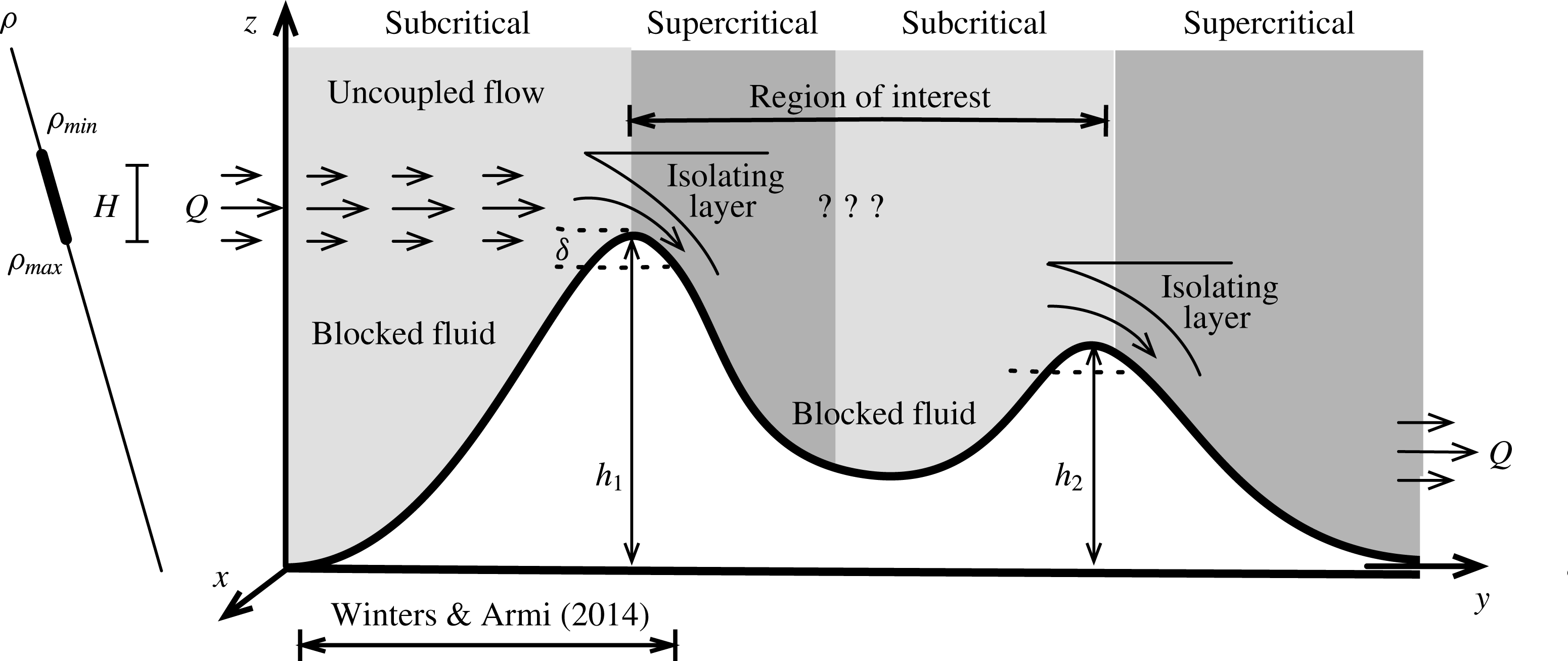
Schematic of stratified flow over a pair of two-dimensional ridges. The flow is hydraulically controlled at the two crests and so undergoes a transition from super- to subcritical flow between the ridges. The blocking heights, a distance
 ${\it\delta}$
beneath the ridge crests, are indicated by the dashed lines. The nature of the internal hydraulic jump is unknown and indicated with the question marks.

Subcritical flow upstream of an obstacle is shaped by upstream topographic influence, i.e. by waves that propagate upstream from the obstacle, communicating its presence and height. The supercritical downslope flow is faster than any long internal wave and is thus insensitive to conditions further downstream, unless or until such conditions are subcritical. In this case, a transition or internal hydraulic jump is required to connect the supercritical downslope flow with a slower, subcritical outflow. The principal focus here is on the changes induced on downslope flows and their transition to a subcritical state by the upstream influence of subcritical conditions further downstream. These conditions are adjusted in the numerical experiments presented here by varying the height of a second obstacle.
A schematic of stratified flow over a pair of two-dimensional ridges is shown in figure 1. Initially and upstream, the flow is uniformly stratified with buoyancy frequency
 $N_{o}$
. We can think of the flow as being drawn through an outlet at a position well beneath the downstream ridge crest at rate
 $Q~\text{m}^{2}~\text{s}^{-1}$
. Though the total flux must also be
 $Q$
, the shape of the inflow velocity profile is not immediately obvious. Intuitively, it seems clear that light fluid from well above the upstream crest will not be drawn all the way down to the outlet location, and neither will dense fluid from well below the crest be drawn up and over both crests. Both would require significant energy to displace fluid vertically against the stable stratification.
To render the experiments numerically feasible, the inflow boundary is placed a finite distance upstream of the obstacle crest. The steady upstream flow can not be specified arbitrarily, however, as it is influenced by upstream propagating waves in a crest-controlled flow. Rather, it should be specified to be dynamically consistent with continuously stratified and sheared hydraulic control at the crest. The analytical form of such an inflow, matching a given
 $N_{o}$
and
 $Q$
in the inviscid, non-diffusive, hydrostatic limit, was found by Winters & Armi (Reference Winters and Armi2014). Here we use that solution as the upstream boundary condition in a finite domain. For uniform
 $N_{o}$
the inflow has a parabolic, jet-like vertical profile. This profile and the density range of the inflowing fluid are indicated in the schematic. Such an inflow produces the optimal, in the sense of minimum energy expenditure, continuously stratified, hydraulically controlled flow over the crest in steady state.
The inflowing jet has a vertical thickness
 $H$
and mean speed
 $U_{o}$
. The flowing layer is displaced downward from the upstream crest height
 $h_{1}$
by the blocking scale
 ${\it\delta}=H/8$
. For simplicity, we take the dynamically uncoupled flow aloft to be motionless. The maximum speed of the jet,
 $U_{max}$
, is equal to
 $3/2\,U_{o}$
with
 $U_{o}=N_{o}H/{\rm\pi}$
. The imposed inflow develops downstream as it passes over the ridge crests and exits as an imposed outflow with matching
 $Q$
at the lower right.
A key feature of the Winters & Armi (Reference Winters and Armi2014) solution is an isopycnal or streamline bifurcation above the location where the blocking depth intersects the upward sloping ridge. The bifurcation, sketched in the schematic, defines a zone of stagnant fluid of uniform density that overlies the accelerating downslope flow. It is the drop in pressure along the descending portion of the bifurcated streamline that reduces the pressure along the topography enough to lift fluid up and over the crest. A bifurcation also develops near the downstream ridge along with a qualitatively similar jet-like flow upstream of the crest control. Bifurcating isopycnals and streamlines are intrinsic to stratified hydraulic control, both at crests and contractions, and are discussed in Wood (Reference Wood1968), Smith (Reference Smith1985) and Winters & Armi (Reference Winters and Armi2012, Reference Winters and Armi2014).
The main objectives of this work are threefold. First, we verify that the idealized optimal upstream flow profiles derived in Winters & Armi (Reference Winters and Armi2014) are consistent with crest-controlled stratified flow when the restrictions of inviscid, hydrostatic flow are relaxed and a no-slip boundary condition is imposed at the topography. Imposing these conditions upstream, we then verify that the fundamental conceptual elements of blocking, bifurcation, and the formation of an isolating layer are indeed dynamically linked to the development of an accelerated downslope flow. Finally, we turn our attention to the flow between the ridge crests and, for a given
 $N_{o}$
,
 $Q$
,
 $H$
and upstream crest height
 $h_{1}$
, to the sensitivity of the flow to the height of the downstream crest. Because the flow is supercritical on the downslope of the upstream ridge and critical at the downstream crest by construction, it must transition somewhere between the crests. Presumably, this transition takes the form of an internal hydraulic jump that depends on the height of the downstream ridge, communicated via the upstream influence of waves originating there. We quantify this influence on the location of the downslope flow separation and on the energy loss in the transition from supercritical to subcritical flow.
2 Modelling approach
The equations of motion for a three-dimensional, stratified fluid in the Boussinesq limit are
 $$\begin{eqnarray}\displaystyle & \displaystyle \frac{\partial }{\partial t}\boldsymbol{u}+\boldsymbol{u}\boldsymbol{\cdot }\boldsymbol{{\rm\nabla}}\boldsymbol{u}+\frac{g}{{\it\rho}_{o}}{\it\rho}^{\prime }\hat{\boldsymbol{z}}=-\frac{1}{{\it\rho}_{o}}\boldsymbol{{\rm\nabla}}p^{\prime }+\mathscr{D}(\boldsymbol{u}) & \displaystyle\end{eqnarray}$$
 $$\begin{eqnarray}\displaystyle & \displaystyle \frac{\partial }{\partial t}{\it\rho}+\boldsymbol{u}\boldsymbol{\cdot }\boldsymbol{{\rm\nabla}}{\it\rho}=\mathscr{D}({\it\rho}). & \displaystyle\end{eqnarray}$$
Here
 $x$
and
 $y$
are horizontal coordinate directions,
 $z$
is vertical, oriented positive upward, and
 $u,v$
and
 $w$
are the corresponding components of the divergence-free velocity vector
 $\boldsymbol{u}$
. The gravitational acceleration
 $g$
acts on small density deviations
 ${\it\rho}^{\prime }$
from a reference value
 ${\it\rho}_{o}$
and
 $p^{\prime }$
is the perturbation pressure.
2.1 The dissipation operator
 $\mathscr{D}$

The
 $\mathscr{D}$
terms combine Laplacian operators, with molecular values
 ${\it\nu}$
for momentum and
 ${\it\kappa}$
for density, with high-order operators with coefficients
 ${\it\nu}_{\ast }$
and
 ${\it\kappa}_{\ast }$
. These latter operators have direct effects that are confined to the smallest scales near the grid resolution. For specificity,
 $$\begin{eqnarray}\mathscr{D}(u)={\it\nu}{\rm\nabla}^{2}u+{\it\nu}_{\ast }\left(\frac{\partial ^{8}}{\partial x^{8}}+\frac{\partial ^{8}}{\partial y^{8}}+\frac{\partial ^{8}}{\partial z^{8}}\right)u.\end{eqnarray}$$
The underlying numerical method is based on Fourier expansions and so the higher-order operators are easily and accurately computed. The coefficients of these operators have dimensions
 $\text{m}^{8}~\text{s}^{-1}$
and are prescribed so that motions at the grid scale have controllable characteristic damping time scales
 $T_{diss}=({\it\nu}_{\ast }k_{\ast }^{8})^{-1}$
, where
 $k_{\ast }$
is the maximum discrete wavenumber. Typically, the damping time is taken to be of the order of 10 time steps. The simulations are spectral large eddy simulations (LES) in the sense that sufficient resolution is used so that the rate of downscale energy cascade is determined by the nearly inviscid dynamics at scales not directly affected by the dissipation operators. In principle, the dissipation rate of kinetic energy
 ${\it\varepsilon}$
should be shown to be independent of moderate changes to the closure coefficients
 ${\it\nu}_{\ast }$
and
 ${\it\kappa}_{\ast }$
. We verify that this is the case by rerunning one simulation (see figure 8) after increasing
 $T_{diss}$
by 50 % and finding no significant change in the mean dissipation rate. A similar approach was used in Winters (Reference Winters2015) for simulations of a stably stratified turbulent boundary layer subject to tidal forcing, with comparable insensitivity to the closure coefficients.
2.2 Boundary conditions
Inflow and outflow are imposed near the up- and downstream boundaries of the computational domain using sponging terms, as discussed in Winters & de la Fuente (Reference Winters and de la Fuente2012). Near the upstream boundary, the fluid is uniformly stratified with buoyancy frequency
 $N_{o}$
over all depths with a parabolic jet inflow of vertical scale
 $H$
and mean speed
 $U_{o}=HN_{o}/{\rm\pi}$
located near the height of the upstream ridge crest. The upstream blocking depth is
 ${\it\delta}=H/8$
and the maximum speed of the jet,
 $U_{max}$
, is
 $3/2U_{o}$
. The density of the inflowing fluid lies between
 ${\it\rho}_{min}$
and
 ${\it\rho}_{max}$
, as indicated in figure 1. The outflow is also specified as a parabolic jet with matching transport, located well beneath the crest of the downstream ridge. The details of the outflow condition are unimportant provided it is such that the flow be controlled at the downstream crest. The upper boundary is a free-slip rigid lid with an adjacent sponge layer imposed to damp the weak upward radiating waves generated by the turbulent fluctuations at the top of the isolating layer. The bottom topography consists of two no-slip, two-dimensional ridges that are treated as a continuous immersed boundary (Winters & de la Fuente Reference Winters and de la Fuente2012; Winters Reference Winters2015).
2.3 Experimental parameters
Equations (2.1) and (2.2) are solved in a cubic domain of size
 $210{\it\delta}$
in the streamwise
 $y$
direction,
 $72{\it\delta}$
in
 $z$
and
 $12{\it\delta}$
in
 $x$
, using a Fourier spectral method with 96, 1681 and 577 equally spaced grid points, respectively. The flow is taken to be periodic in the statistically homogeneous, cross-stream direction. The dimensionless parameters for all runs are
 $N_{o}H/{\rm\pi}U_{o}=1$
,
 $Re=U_{o}H/{\it\nu}=1.1\times 10^{6}$
and
 ${\it\nu}/{\it\kappa}=1$
. Because the simulations are well-resolved LES, as demonstrated in appendix A, the values of
 ${\it\nu}$
and
 ${\it\kappa}$
are small enough that they have essentially no influence on the solutions. The value of
 $N_{o}H/{\rm\pi}U_{o}$
ensures that the sheared inflow is subcritical with respect to long gravity waves and matches the optimal, crest-controlled flow derived in Winters & Armi (Reference Winters and Armi2014). The dimensionless time step
 $\text{d}tU_{o}/H$
is of the order of
 $10^{-4}$
. The scaled height difference between the two ridges,
 ${\it\Delta}=(h_{1}-h_{2})/H>0$
, is the control parameter that is varied between runs.
2.4 Two-dimensional spin-up
The experiments are started from rest with an initial buoyancy frequency
 $N_{o}$
. The flow is then smoothly and rapidly forced to match the prescribed in- and outflow conditions via relaxation terms applied within the up- and downstream sponge regions. The interior flow responds to the imposition of these conditions and is allowed to adjust according to (2.1) and (2.2), albeit constrained to two dimensions by setting the cross-stream gradients of all quantities equal to zero. The nominal fluid transit time,
 $T_{transit}=D/U_{o}$
, is approximately 8.5 buoyancy periods
 $2{\rm\pi}/N_{o}$
, where
 $D$
is the horizontal separation between the ridges. This initial two-dimensional development of the flow is computed for approximately
 $2T_{transit}$
. During this time, hydraulic controls are established at both ridge crests. The details of the flow between the crests, however, are not captured accurately in the spin-up phase because the strongly sheared downslope flow exhibits numerous shear instabilities that are not physically constrained to evolve in two spatial dimensions.
2.5 Quasisteady, three-dimensional turbulent flow
Three-dimensional simulations are required to characterize the quasisteady, turbulent flow that transitions from a supercritical state on the downslope of the upstream ridge to a subcritical state approaching the crest of the downstream ridge. For several values of
 ${\it\Delta}$
, initial two-dimensional spin-up calculations are run as described above. Snapshots of the two-dimensional flow fields are then spread across the three-dimensional domain, along with a random, three-dimensional perturbation of the velocity field with a characteristic amplitude of
 $U_{o}/1000$
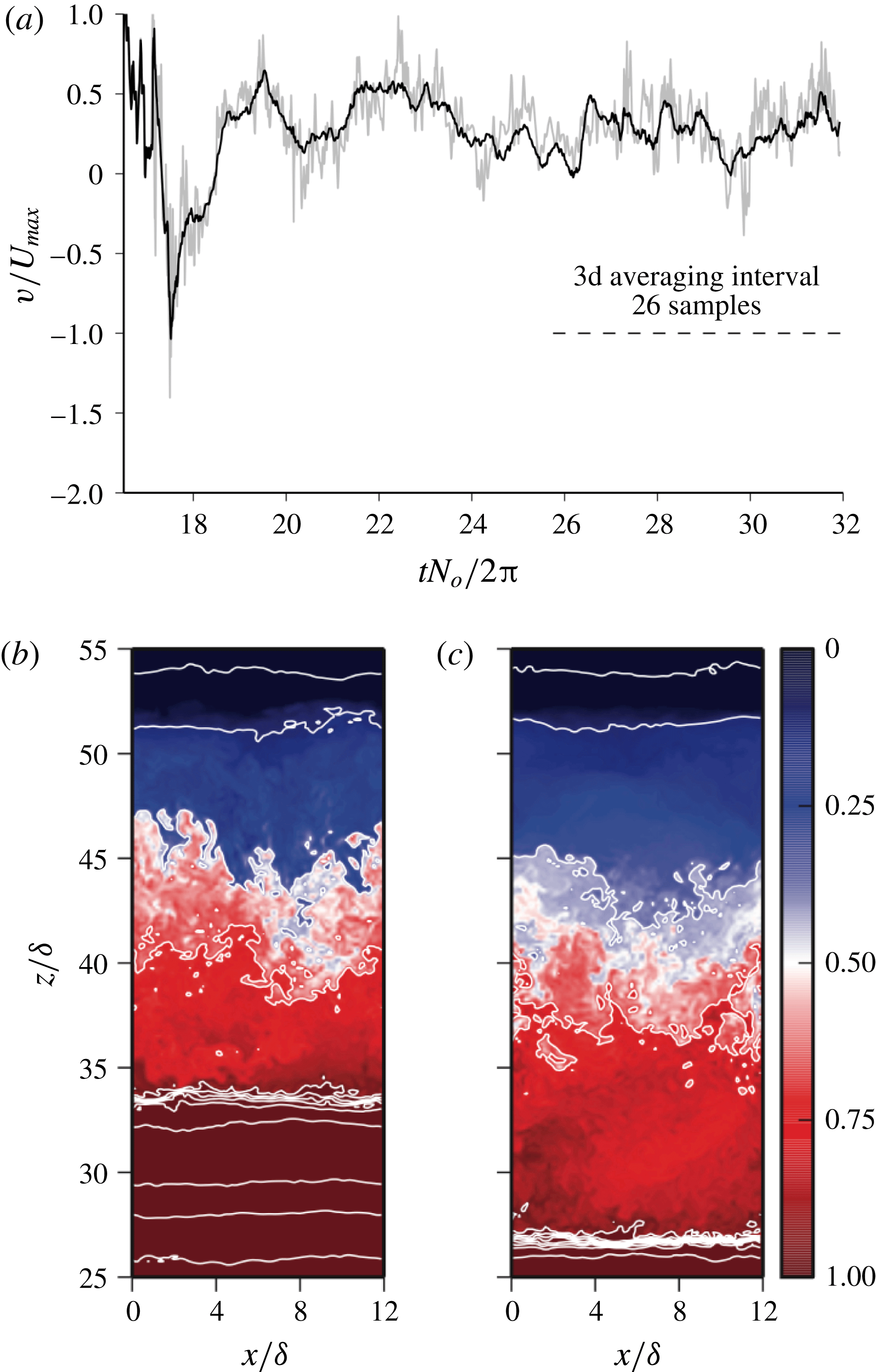
. These perturbed, nominally two-dimensional flow fields are then allowed to evolve under the fully three-dimensional equations (2.1) and (2.2). The flow rapidly transitions to a three-dimensional state. Figure 2 shows the time series of the streamwise speed
 $v$
at a fixed point (indicated in figure 6) as well as the cross-stream average of the same quantity for the case
 ${\it\Delta}=2.10$
after the two-dimensional spin-up phase. During the first buoyancy period, the two signals are indistinguishable, as three-dimensional motions have not yet reached finite amplitude. After this short transition period, the pointwise and cross-stream-averaged signals are correlated but distinctly different. Our later analyses will be confined to the quasisteady portion of the flow, indicated here by the averaging interval with
 $t$
greater than approximately 26 buoyancy periods with 26 temporal samples. We describe the flow as quasisteady because, while the upstream flow is essentially steady, the flow in the region of interest between the sill crests is turbulent, owing to the multiple shear instabilities both on the upper flank of the downslope flow and downstream of its separation from the upstream ridge. The three-dimensional nature of the flow can also be seen in the cross-stream structure of the density field shown in the figure 2(c).
(a) Time series of
 $v$
(grey) for
 ${\it\Delta}=2.10$
at
 $x=0$
,
 $y/{\it\delta}=86.5$
and
 $z/{\it\delta}=30$
. The
 $x$
-averaged value
 $\bar{v}$
at the same
 $y$
and
 $z$
location (dark). (b,c) Cross-stream density
 $({\it\rho}-{\it\rho}_{min})/({\it\rho}_{max}-{\it\rho}_{min})$
for
 ${\it\Delta}=1.26$
(b) and
 ${\it\Delta}=2.10$
(c) shown in colour. Equally spaced contours (white) are also shown. These extend over a wider range of values than shown in the colour scale, which is restricted to the inflow range
 $0\leqslant ({\it\rho}-{\it\rho}_{min})/({\it\rho}_{max}-{\it\rho}_{min})\leqslant 1$
.

3 Results
3.1 Adjusted flow approaching the upstream crest
At
 $y=0$
, the inflow velocity and density profiles are prescribed to match the optimal controlled flow for a specified stratification
 $N_{o}$
and total flux
 $Q$
. In theory, this flow should be drawn up over a ridge crest at a height
 ${\it\delta}$
above the lowest flowing streamline, and subsequently be accelerated in a downslope flow beneath a nearly stagnant isolating layer. In deriving this upstream solution, several simplifying approximations were made: the flow was assumed to be hydrostatic, inviscid and non-diffusive, and the ridge was modelled using a free-slip boundary condition. In the numerical simulations, however, the fluid is both viscous and diffusive, and a no-slip boundary condition is imposed along the bottom topography. Moreover, both long and short gravity waves can be excited, as the underlying equations are non-hydrostatic. The imposed inflow conditions thus represent an approximation to the steady flow approaching the upstream ridge crest that would be obtained under a less restrictive set of dynamical constraints. The nature and magnitude of the adjustments to the flow approaching the crest that stem from relaxing these constraints are of interest.
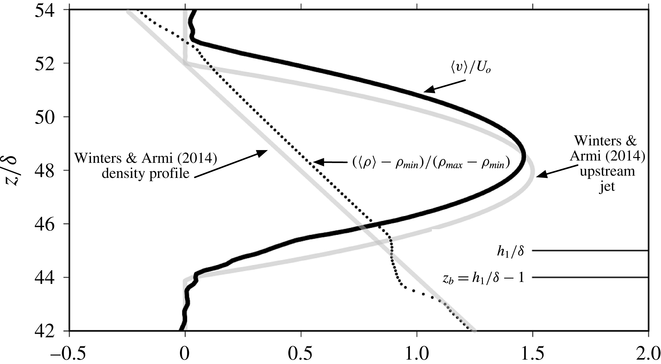
Figure 3 shows vertical profiles of the approach flow
 $v$
and density
 ${\it\rho}$
, averaged in
 $x$
at approximately
 $y/{\it\delta}=25$
, slightly upstream of the point where the topography intersects the blocking depth
 $h_{1}-{\it\delta}$
(see figure 4). Also shown are the idealized, optimal profiles derived in the inviscid limit. Because the approach flow is subcritical, there is upstream influence of the topography. This influence is carried by long gravity waves in the theoretical derivation, and gravity waves of any scale in the numerical solutions. If the theory were incorrect to first order, a significant adjustment would have to occur between
 $y=0$
, and the first ridge crest and the idealized and simulated profiles would differ significantly. Rather, we see only a relatively small adjustment, and the approach flow shares the main qualitative features of the Winters & Armi (Reference Winters and Armi2014) solution. Both approach flows are jet-like, with speed maxima of approximately
 $3/2\,U_{o}$
. In both flows, the density gradient is approximately uniform with
 $N\approx N_{o}$
, though the stratification is perturbed somewhat near the upper and lower edges of the jet in the simulated flow. Comparing the analytical and numerical solutions, it appears that the main deficiency of the idealized solution stems from the neglect of viscosity, and thus the no-slip boundary condition. With a no-slip condition, the approach flow has its maximum speed reduced by approximately 3 % and is displaced upward approximately
 $1{\it\delta}$
.
Instantaneous spanwise (
 $x$
) averaged profiles of
 $v$
(dark, solid) and
 ${\it\rho}$
(circles) at
 $y/{\it\delta}\approx 25$
in the quasisteady regime for
 ${\it\Delta}=0.84$
shown in figure 4. Also shown are the idealized, analytical profiles derived in Winters & Armi (Reference Winters and Armi2014) and used as inflow conditions at
 $y=0$
.

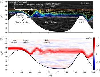
(a) Instantaneous isopycnals at
 $x=0$
in the quasisteady regime for
 ${\it\Delta}=0.84$
. Density values corresponding to the range of values that inflow at
 $y=0$
are coloured while all other values are shown in grey. (b) The corresponding normalized speed.

The lack of significant adjustment and change in character of the approach flow is strong evidence that the upstream influence of waves in continuously stratified, crest-controlled flows acts to block the flow beneath a height
 $h_{1}-{\it\delta}$
and shape the inflow profile into a jet. It is interesting to note that the average speed of the inflowing layer, with thickness
 $H=8{\it\delta}$
, is equal to
 $U_{o}=N_{o}H/{\rm\pi}$
, the speed of long gravity waves in an unsheared flow of equal transport and thickness. Such a uniform flow is exactly critical to waves of vertical scale
 $H$
, and supercritical to all smaller waves. It would therefore prevent any upstream influence and would not be topographically controlled at the crest. In contrast, a sheared, jet-like profile with the same transport, as we observe here, is subcritical to long waves of vertical scale
 $H$
, so upstream influence does occur and the approach flow can be hydraulically controlled at the crest.
3.2 Qualitative flow features
The Winters & Armi (Reference Winters and Armi2014) derivation of continuously stratified, optimal, topographically controlled flow is mathematically rather simple; it simply involves integrals of Bernoulli’s equation, yet it relies heavily on a particular conceptual framework which renders the mathematics straightforward. Fundamentally, this theory posits the existence of flow asymmetry or hydraulic control at a ridge crest. Intrinsic to the supercritical flow downstream of the crest is upstream blocking and a streamline and isopycnal bifurcation that forms at the upper edge of the controlled, flowing layer just upstream of the crest. The bifurcation forms a stagnant isolating layer of uniform density above the accelerated downslope flow. We have seen in the previous section that this theory provides a good prediction of the upstream influence and the subcritical approach flow conditions. If this flow is imposed as an upstream boundary condition, then consistency of the analytical theory implies that a streamline/isopycnal bifurcation should develop and that an isolating layer will develop. The subsequent alteration of the pressure field should then draw fluid up and over the ridge crest and form an accelerating downslope flow. We have no way of imposing these flow developments on the numerical solutions. Rather, with the specified inflow conditions, the simulations provide a consistency check on the conceptual elements used to construct the theory. In addition, the simulations are non-hydrostatic, so short wavelength shear instabilities, neglected in the theory, can occur and provide a transition to turbulent flow. The no-slip condition also allows the possibility of an adverse pressure gradient and flow separation in the lee.
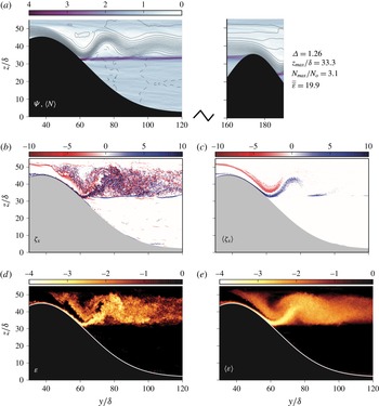
Figure 4 shows a two-dimensional snapshot of the quasisteady flow for
 ${\it\Delta}=0.84$
. Animations of these images are included as supplementary movies available online at http://dx.doi.org/10.1017/jfm.2016.113. The various flow features depicted in figure 1 and used to construct the solutions in Winters & Armi (Reference Winters and Armi2014) are visible and highlighted in the image. Density contours within the inflow range
 ${\it\rho}_{min}\leqslant {\it\rho}\leqslant {\it\rho}_{max}$
are contoured with uniform spacing from red to blue. Density values outside this range are contoured with the same increment in grey. The uppermost inflowing density contour bifurcates just above the blocking point that separates upstream fluid that will overflow the ridge from the blocked fluid beneath. The bifurcation defines a nearly stagnant pool of fluid with approximately uniform density that isolates the strongly stratified downslope flow adjacent to the boundary from the fluid aloft that maintains its initial stratification. The downslope flow separates from the obstacle and rebounds upward, forming what appears to be an internal hydraulic jump.
Downstream of the jump, the flow is thicker, slower, and more weakly stratified than it was either initially or near the separation point. This flow forms the subcritical, jet-like inflow for the downstream ridge. Because the imposed outflow conditions require the flow to be asymmetric across the second ridge, a second hydraulic control forms at the downstream crest. The flow there is qualitatively similar to the flow at the upstream crest, but differs in detail owing to changes in the stratification relative to the inflow. The flow is blocked below a small offset from the downstream crest, creating a pool of dense, stratified fluid that is trapped between the two ridges. This pool is capped by a thin layer with markedly increased stratification linking the blocking point on the upslope of the downstream ridge with the separation point on the downslope of the upstream ridge.
3.3 Mean transport and stratification
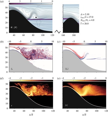
The structure of the time-averaged, two-dimensional flow,
 ${\it\Delta}=1.26$
and
 ${\it\Delta}=2.10$
, is shown in figures 5 and 6 at
 $x=0$
. The same equally spaced contours of the streamfunction
 ${\it\Psi}(y,z)$
, where
 $\langle v\rangle =\partial {\it\Psi}/\partial z$
and
 $\langle w\rangle =-\partial {\it\Psi}/\partial y$
, are shown for both cases in panel (a). From here on, angle brackets are used to indicate time averaging in the quasisteady regime as shown in figure 2. The streamwise transport occupies a stream tube that separates from the upstream ridge and oscillates vertically as it broadens and slows downstream. The separation height coincides with a thin layer of significantly enhanced stratification
 $\langle N\rangle$
, normalized by the inflow stratification
 $N_{o}$
and shown in colour. The approximate position and buoyancy frequency of this layer are denoted
 $z_{max}$
and
 $N_{max}$
, respectively, quantified with respect to vertical profiles at
 $y/{\it\delta}=120$
. The separation height closely matches the downstream blocking height in both cases, with the coincident locations established and maintained by gravity waves propagating along the strongly stratified interface. Increasing
 ${\it\Delta}$
by reducing the downstream crest height
 $h_{2}$
reduces both the downstream blocking height and the height of flow separation.
(a) Equally spaced contours of the time-averaged, two-dimensional streamfunction
 $\langle {\it\Psi}(y,z)\rangle$
. The mean buoyancy frequency
 $\langle N(y,z)\rangle$
is shown in colour. Both quantities are normalized by
 $N_{o}$
. (b,c) Instantaneous and time-averaged cross-stream vorticity
 ${\it\zeta}_{x}$
, also scaled by
 $N_{o}$
. (d,e) Corresponding dissipation rate of kinetic energy
 ${\it\varepsilon}$
scaled by
 $U_{o}^{3}/{\it\delta}$
. All slices taken at
 $x=0$
for the case
 ${\it\Delta}=1.26$
.

Compared to the inflow stratification, the downslope flow is more strongly stratified, while the stratification of the flow downstream of the jump is significantly weakened. In both cases, a pronounced nearly stagnant, nearly unstratified isolating layer separates the downslope flow from the passive, stratified flow aloft upstream of the separation point and the internal hydraulic jump.
A simple argument appears to explain both the position and the strength of the sharp density interface. Take
 $z_{max}\approx h_{2}$
, the height of the downstream ridge. For all cases, this is accurate to
 $O({\it\delta})$
, which, at low Froude number
 $U_{o}/N_{o}h_{i}$
, is much smaller than either
 $h_{1}$
or
 $h_{2}$
, and also significantly smaller than
 $H$
. In the lee of the upstream ridge, the fluid between
 $z=h_{1}-{\it\delta}$
and
 $z_{max}\approx h_{2}$
is initially uniformly stratified, with buoyancy frequency
 $N_{o}$
. The overflow displaces this fluid downward and compresses it into a layer of thickness
 $O({\it\delta})$
. The density range between these heights is thus compressed vertically by a factor of approximately
 $(h_{1}-h_{2}-{\it\delta})/{\it\delta}$
, resulting in a sharp pycnocline with
 $N\approx \sqrt{(h_{1}-h_{2}-{\it\delta})/{\it\delta}}N_{o}$
. To illustrate, for the case
 ${\it\Delta}=1.26$
, the factor
 $\sqrt{(h_{1}-h_{2}-{\it\delta})/{\it\delta}}$
is equal to 3.02, which is in good agreement with the computed value
 $N_{max}=3.1N_{o}$
.
As in figure 5 but for
 ${\it\Delta}=2.10$
.

Immediately after separation, the mean flow ascends and then descends again towards the sharp pycnocline. This flow pattern surrounds a recirculation zone below that is strongly turbulent owing to the high bottom shear along the topography. This feature is reminiscent of atmospheric rotors commonly observed in the lee of mountains when the approach Froude number is large, see e.g. Doyle & Durran (Reference Doyle and Durran2002). In those flows, the downslope flow penetrates all the way to the ground, before ascending and descending in a wave-like pattern. For the low-Froude-number flows considered here, the downslope flow separates well above the ground, and the sharp pycnocline acts as an interior barrier that confines an intense rotor within the fluid interior.
3.4 Turbulent flow features
Figures 5(b–e) and 6(b–e) suggest that both the near homogenization of the isolating layer and the weakened stratification in the downstream flowing layer are the result of turbulent mixing originating along the highly sheared flanks of the jet-like flowing layer. Instantaneous and time-averaged views of the
 $x$
component of vorticity,
 ${\it\zeta}_{x}$
, normalized by
 $N_{o}$
, are shown. Values with
 $|{\it\zeta}_{x}|/N_{o}<2$
are removed to highlight the highly sheared portion of the flow. The instantaneous fields exhibit a chaotic mix of small-scale features with vorticity of both signs, as well as larger features that appear to be the modes of instability along the upper flank of the attached downslope flow. These turbulent fluctuations are nearly completely removed by time averaging. On average, the jet-like flow has strong vorticity of opposite signs on either flank. Downstream of the separation point, the mean vorticity is strongest along the lower flank, and this shear appears to be a significant source of the small-scale motions in the lee. For the larger value
 ${\it\Delta}=2.10$
, the cloud of turbulent eddies penetrates to greater depth and appears to be more intense. The cross-stream structure of the flow for these cases is shown in figure 2 and the location of the time series in that figure is indicated by the black dot in figure 6(a).
Figures 5(d,e) and 6(d,e) show the corresponding dissipation rate,
 ${\it\varepsilon}$
, defined in appendix A, both instantaneously and after time averaging. The highest values occur in the fast, upward flowing stream just after it separates from the upstream ridge. Like the vorticity, the penetration depth and intensity of the signal is comparatively larger for larger
 ${\it\Delta}$
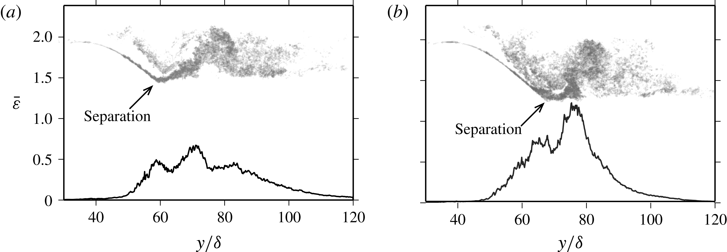
. Overall, the spatial patterns are similar to those of the vorticity field and the dissipation rate decreases markedly with distance after the flowing stream reaches its maximum height. The streamwise structure of the dissipation,
 $\bar{{\it\varepsilon}}$
, is shown in figure 7 for
 ${\it\Delta}=[1.26,2.10]$
, where
 $$\begin{eqnarray}\bar{{\it\varepsilon}}(y)=\frac{1}{U_{o}^{3}}\int \langle {\it\varepsilon}(x_{o},y,z)\rangle \,\text{d}z\end{eqnarray}$$
and the integral extends from the topography to
 $z/{\it\delta}=55$
. Except in magnitude, the structure for other values of
 ${\it\Delta}$
is similar. For both cases shown, the maximum dissipation rate occurs downstream of the separation point and appears to be associated with the strong negative vorticity on the underside of the upward flow just after separation. A significant fraction of the total occurs upstream of the separation point, which underscores the importance of the instabilities excited along the bottom edge of the isolating layers.
3.5 Dependence on
${\it\Delta}$

Bulk properties of the turbulent flow between the two ridges were computed for different downstream ridge heights
 $h_{2}$
corresponding to
 ${\it\Delta}=[0.42,0.84,1.26,1.68,2.1,3.3]$
. These quantities are shown in figure 8. The quantity
 $z_{max}/{\it\delta}$
quantifies both the separation height from the upstream ridge and the blocking height of the downstream ridge. This height decreases monotonically, though not linearly, with increasing
 ${\it\Delta}$
. The circled values correspond to the specific cases shown in figures 5 and 6. Conversely, the corresponding maximum stratification
 $N_{max}/N_{o}$
, which occurs in a thin layer at the separation and blocking depth, increases with increasing
 ${\it\Delta}$
. The spatially integrated, time-averaged dimensionless dissipation rate is defined as
 $$\begin{eqnarray}\bar{\bar{{\it\varepsilon}}}=\frac{1}{{\it\delta}U_{o}^{3}}\iint \langle {\it\varepsilon}(x_{o},y,z)\rangle \,\text{d}y\,\text{d}z,\end{eqnarray}$$
where
 $30\leqslant y/{\it\delta}\leqslant 120$
. As
 ${\it\Delta}$
increases, and the downslope flow penetrates to greater depth, the total energy dissipated also increases, at least over the range of values simulated, though there appears to be a significant flattening of the curve with increasing
 ${\it\Delta}$
. Most of the increase in dissipation with
 ${\it\Delta}$
occurs downstream of the separation point and is associated with an intensification of the rotor-like feature that is produced by the sheared, upward flow. This trend can be seen by comparing figures 5 and 6.


(a) Height of the time-averaged stratification maxima,
 $z_{max}/{\it\delta}$
, measured at
 $y/{\it\delta}=120$
as a function of dimensionless topographic height difference
 ${\it\Delta}$
. This height closely corresponds to both the separation point from the upstream ridge and the blocking height at the downstream ridge. (b) The corresponding scaled maximum stratification,
 $N_{max}/N_{o}$
. (c) The time-averaged, dimensionless dissipation rate,
 $\bar{\bar{{\it\varepsilon}}}$
, integrated over the dimensionless spatial domain shown in figures 5(d,e) and 6(d,e). Circled symbols are cases shown in figures 2 and 5–7. Dashed lines give the best quadratic fit to the discrete data points.

The dissipative losses associated with the transition from super- to subcritical flow are moderate compared to the work done on the fluid by the pressure drop associated with the isopycnal bifurcation and formation of the isolating layer. This work,
 $\mathscr{P}\mathscr{V}$
, is given by
 $$\begin{eqnarray}\mathscr{P}\mathscr{V}=\frac{1}{{\it\delta}U_{o}^{3}}\frac{1}{{\it\rho}_{o}}\int \langle pv|_{y_{c}}-pv|_{y_{s}}\rangle \,\text{d}z,\end{eqnarray}$$
where the integral is evaluated at
 $x_{o}$
from the topography to
 $z/{\it\delta}=55$
, as in (3.2), at the streamwise positions
 $y_{c}$
and
 $y_{s}$
, which denote the positions of the ridge crest and the separation point, respectively. For the flows shown in figures 5 and 6,
 $\bar{\bar{{\it\varepsilon}}}$
is only 10–15 % of
 $\mathscr{P}\mathscr{V}$
. A much larger fraction of
 $\mathscr{P}\mathscr{V}$
, 80–90 % is converted to work done by the downslope flow,
 $\mathscr{B}\mathscr{F}$
, as it displaces relatively light fluid downward, forming the sharp pycnocline. This work is estimated as
 $$\begin{eqnarray}\mathscr{B}\mathscr{F}=\frac{1}{{\it\delta}U_{o}^{3}}\frac{-g}{{\it\rho}_{o}}\iint \langle {\it\rho}^{\prime }w\rangle \,\text{d}y\,\text{d}z,\end{eqnarray}$$
using the same limits of integration as in (3.3).
4 Discussion
A blocked, crest-controlled, stratified flow is simulated numerically as it overflows a two-dimensional ridge. As predicted theoretically (Winters & Armi Reference Winters and Armi2014), the flow transitions from a subcritical jet upstream of the obstacle to an accelerating, supercritical downslope flow beneath a nearly stagnant, nearly homogeneous isolating layer that develops as the flow approaches a quasisteady state. The downslope flow is highly sheared at its upper edge, where it meets the isolating layer, giving rise to instabilities and three-dimensional turbulence. The downslope flow separates from the ridge, and spawns further instabilities and turbulent motions along its lower edge owing to strong shear of opposite sign.
The downstream outflow is prescribed beneath the blocking depth
 $h_{2}-O({\it\delta})$
of the downstream ridge, so the overflow there must be asymmetric and controlled at the crest. This implies that, upstream of the downstream crest, the flow is subcritical. The imposed inflow, upstream of the upstream crest, is dynamically consistent with optimal, controlled flow at that crest. The supercritical downslope flow that results must connect to the subcritical flow approaching the downstream ridge, thus ensuring a transition from supercritical to subcritical states between the ridges, i.e. the formation of an internal hydraulic jump.
The overall flow would be qualitatively different if the two ridge heights were the same. In this case, neglecting the effects of viscosity, the imposed upstream conditions are consistent with control at the upstream ridge crest. Rather than transitioning to a supercritical state, however, the flow would be symmetric across that crest, returning to the prescribed subcritical upstream conditions further downstream. The same symmetric response would occur at the downstream ridge, provided that the imposed outflow was chosen appropriately, i.e. matching the inflow. If, on the other hand, the outflow was specified at a depth lower than
 $h_{2}-{\it\delta}$
, the flow would be asymmetrical across the downstream crest, and thus transition to a supercritical state.
If the downstream ridge were taller than
 $h_{1}+{\it\delta}$
, then the first ridge would be beneath the blocking depth of the second ridge. The optimal upstream flow consistent with control at the taller downstream ridge would be unaffected by the presence of a shorter upstream ridge. For flows in the small-Froude-number limit, i.e. where the blocking scale
 ${\it\delta}$
is small compared to the obstacle height, tall obstacles shield the flow from the effects of shorter topography upstream.
Finally, in the limit
 $h_{2}\rightarrow 0$
, the downstream control is removed and the problem is no longer uniquely specified. The fate of the downslope flow is then determined directly by the imposed outflow conditions, which could be specified arbitrarily, provided that the net transport is equal to
 $Q$
. For specified upstream conditions, there is no uniquely distinguished flow in the lee of the ridge in this case. For example, supercritical flow specified near
 $z=0$
would suppress a transition from super- to subcritical flow, while subcritical flow specified over any depth range would determine the nature of the jump required. The presence of a downstream ridge with a deep outflow further downstream renders the flow between the ridges unique by establishing the subcritical flow that determines the form of the jump further upstream.
In these experiments, we prescribed
 $0<h_{2}<h_{1}-{\it\delta}$
in order to examine the unique flows between the ridge crests that transition from a supercritical to a subcritical state. For identical flow conditions at
 $y=0$
and at the upstream crest, the depth of separation and the intensity of the turbulent mixing downstream of the crest depend on the subcritical flow conditions upstream of the downstream ridge, which are determined by its height. The presence and height of the downstream ridge are communicated upstream via gravity waves that propagate on the strong pycnocline that develops, separating the flowing stream from the blocked, stratified pool between the ridges at depth. The position of the pycnocline coincides with the depth of separation upstream. The penetration depth of the downslope flow, the strength of the strong pycnocline, and the total kinetic energy dissipated between the ridge crests all increase with the normalized height difference
 ${\it\Delta}$
.
The results demonstrate and extend recently developed concepts in continuously stratified, crest-controlled flows. Hydraulic theory relies on the simplifying idealizations of inviscid and non-diffusive hydrostatic flow. It does not specifically address the excitation and consequences of non-hydrostatic, parasitic instabilities occurring either at the upper edge of the downslope flow itself or after separation from the topography. Instabilities and turbulence have, however, been invoked as a mechanism for changing the state of a flow from subcritical to supercritical (Liu, Thorpe & Smyth Reference Liu, Thorpe and Smyth2012). Triggered by shear instabilities, supercritical downslope flows suffer irreversible energy losses well prior to flow separation and any transitions loosely analogous to hydraulic jumps. These losses are comparable to the losses incurred after flow separation, and complicate prediction of the degree of supercriticality of the flow prior to transition. The results presented illustrate the spatial character of the turbulent transition in these flows and their sensitivity to downstream conditions.
Acknowledgements
This work was supported by the National Science Foundation, grant nos OCE-1061027 and AGS-1540585. XSEDE computing resources were made available under grant TG-OCE120004.
Supplementary movies
Supplementary movies are available at http://dx.doi.org/10.1017/jfm.2016.113.
Appendix A
Assuming a downscale energy transfer through an inertial subrange, the local kinetic energy transfer rate
 ${\it\varepsilon}$
is estimated as the rate at which the dissipative terms in (2.1) and (2.2) remove kinetic energy:
 $$\begin{eqnarray}{\it\varepsilon}={\it\nu}(|\boldsymbol{{\rm\nabla}}u|^{2}+|\boldsymbol{{\rm\nabla}}v|^{2}+|\boldsymbol{{\rm\nabla}}w|^{2})+{\it\nu}_{\ast }\mathop{\sum }_{i=1}^{3}\left[\left(\frac{\partial ^{4}u}{\partial x_{i}^{4}}\right)^{2}+\left(\frac{\partial ^{4}v}{\partial x_{i}^{4}}\right)^{2}+\left(\frac{\partial ^{4}w}{\partial x_{i}^{4}}\right)^{2}\right]\!.\end{eqnarray}$$
Here
 $x_{i}$
, for
 $i=1,2,3$
refers to the
 $x$
,
 $y$
and
 $z$
coordinates respectively. The high-order derivative operators, which act only at scales near the grid resolution by design, allow a substantial inertial subrange where nonlinear, nearly inviscid physics sets the rate of downscale energy transfer
 ${\it\varepsilon}$
. Ultimately, energy and density variance are removed from the calculation by these operators upon arrival at the smallest grid scales.
This treatment of the dissipative terms renders the calculations a form of LES with the explicit ‘closure’ parameter
 ${\it\nu}_{\ast }={\it\kappa}_{\ast }$
. As for all LES, it is necessary to argue, and desirable to demonstrate, that the results obtained are insensitive to, or at least not fundamentally altered by, reasonable changes in the values of any ad hoc closure parameters (e.g. Mason Reference Mason1994). Here the value of
 ${\it\nu}_{\ast }$
is prescribed so that motions at the grid scale have damping time scales
 $T_{diss}$
of the order of a few to several time steps, typically approximately 10.
For the particular simulation with
 ${\it\Delta}=1.68$
, the three-dimensional portion of the simulation was rerun after decreasing
 ${\it\nu}_{\ast }$
by a factor of
 $2/3$
, and thus increasing
 $T_{diss}$
by 50 %, leaving all other parameters of the simulation unchanged. The integrated dissipation rate
 $\bar{\bar{{\it\varepsilon}}}$
was nearly unchanged in this sensitivity test, and is shown in figure 8 as the white circle. This confirms the experimental design principle that the rate of the downscale cascade of kinetic energy
 ${\it\varepsilon}$
be determined by nearly inviscid dynamics at scales that are insensitive to the precise form of the dissipation operators.