1 Introduction
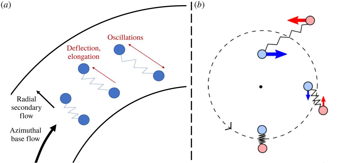
Viscoelastic fluids can be obtained by adding a small amount of high-molecular-weight polymer molecules to Newtonian solvents. When sheared, viscoelastic fluids are characterised by viscous dissipation and elastic redistribution of energy through entropic forces (Bird, Armstrong & Hassager Reference Bird, Armstrong and Hassager1987a ; Bird et al. Reference Bird, Curtiss, Armstrong and Hassager1987b ). The viscoelastic instability (VEI) results from the destabilisation of a viscoelastic flow at low Reynolds number when the elasticity of the polymer solution is competing against the viscous dissipation (Larson Reference Larson1992). It may even occur at vanishing Reynolds number and is then called the ‘purely elastic instability’, as discovered by Larson, Shaqfeh & Muller (Reference Larson, Shaqfeh and Muller1990) in Taylor–Couette flow. For viscoelastic flows of a constant-viscosity solution, the total stress tensor can be decomposed into a sum of the Newtonian stress tensor for the solvent and the polymeric stress tensor which is governed by the Oldroyd-B equation (Morozov & van Saarloos Reference Morozov and van Saarloos2007). The flow regimes of viscoelastic flows depend mainly on the two control parameters: the Reynolds number Re, which is the ratio between the viscous characteristic time and the inertia characteristic time; and the Weissenberg number Wi, which is the ratio of the polymer relaxation time and the inertia characteristic time. The ratio between the viscous diffusion time and the relaxation time defines the elasticity E of the solution. Flows of viscoelastic solutions can become unstable to inertia-induced perturbations for very weak values of E or to inertio-elastic perturbations for intermediate values of E and to purely elasticity-driven perturbations for large values of E. In their analysis, Larson et al. (Reference Larson, Shaqfeh and Muller1990) provided an intuitive explanation of viscoelastic instability using an ‘elastic dumbbell’ model, as shown in figure 1(a). Flow perturbations in the radial direction deflect the dumbbells while they stretch them in the azimuthal base flow. This creates an elastic restoring force which competes against the deflecting curvature. If the spring constant is small enough (i.e. the relaxation time of the polymer is high), the distance between the beads will keep growing, leading to an instability in the form of growing oscillations. This instability mechanism was later supported by experimental findings (Groisman & Steinberg Reference Groisman and Steinberg1998). The VEI has been experimentally, numerically and theoretically probed in many works, as reviewed by Groisman & Steinberg (Reference Groisman and Steinberg1996). In particular, several regimes of viscoelastic flows in the Taylor–Couette system (i.e. flow in the gap between two coaxial differentially rotating cylinders) have been investigated, leading to various thresholds and instability modes depending on the solvent and the polymer concentration (Shaqfeh Reference Shaqfeh1996; Beaumert & Muller Reference Beaumert and Muller1999; Crumeyrolle, Mutabazi & Grisel Reference Crumeyrolle, Mutabazi and Grisel2002; Latrache, Crumeyrolle & Mutabazi Reference Latrache, Crumeyrolle and Mutabazi2016).
(a) As discussed by Larson et al. (Reference Larson, Shaqfeh and Muller1990), ‘elastic dumbbells’ provide an intuitive explanation of the mechanism of viscoelastic destabilisation of a Taylor–Couette flow. (b) Intuitive explanation of the MRI in terms of elastic dumbbells (see https://www.cfa.harvard.edu/∼namurphy/Lectures/Ay253_07_MHDinstabilities2.pdf).

The intuitive interpretation of the VEI in terms of a ‘dumbbell’ model brings this phenomenon close to the magnetorotational instability (MRI), which is believed to cause the destabilisation of astrophysical accretion disks. Although the circulation Rayleigh criterion ensures that an inviscid circular flow is stable in the Keplerian regime so that it cannot trigger turbulence alone (Balbus & Hawley Reference Balbus and Hawley1998; Ji et al. Reference Ji, Burin, Schartman and Goodman2006), the presence of a weak axial magnetic field can destabilise a conducting flow, as first discovered by Velikhov (Reference Velikhov1959) and Chandrasekhar (Reference Chandrasekhar1960) in the context of laboratory hydrodynamics and then by Balbus & Hawley (Reference Balbus and Hawley1991) in the context of accretion disks. In order for a magnetised flow to be stable, the angular velocity should increase outwards, and crucially this is violated for a Keplerian flow. It is now believed that the MRI is a key phenomenon that drives momentum transport in accretion disks. The MRI can be explained in terms of elastic dumbbells, as displayed in figure 1(b). The presence of a magnetic field induces an elastic force between two fluid elements while the differential rotation stretches the spring linking them, and the restoring force slows down the bead on the inner orbit. The deformation of the magnetic field induces a magnetic tension on the dumbbell which destabilises the system. The MRI may be caused by the presence of an axial field (‘standard MRI’), or an azimuthal field (‘azimuthal MRI’) or both (‘helical MRI’) (Hollerbach & Rüdiger Reference Hollerbach and Rüdiger2005).
The physical mechanisms causing the destabilisation of a conducting flow in the MRI and a viscoelastic flow in the VEI are very similar. The analogy was formalised by Ogilvie & Proctor (Reference Ogilvie and Proctor2003) who noticed that the constitutive equation describing a polymer solution of infinite relaxation time in the Oldroyd-B model is identical to the equation satisfied by Maxwell’s stress tensor in ideal magnetohydrodynamics (MHD) (see § 2). They decomposed the polymeric stress tensor in terms of three magnetic-like fields. Away from the limit of infinite relaxation time, the decomposition could not be done with fewer than three fields, which is reminiscent of the fact that the analogy between the constitutive equations of the Oldroyd-B model and the MHD equations is not exact. This issue was not further investigated. Ogilvie & Potter (Reference Ogilvie and Potter2008) performed a linear stability analysis for the viscoelastic Taylor–Couette system in order to probe this analogy, observing that the VEI modes at high Weissenberg number were similar to that of the azimuthal MRI in a perfectly conducting fluid. Boldyrev, Huynh & Pariev (Reference Boldyrev, Huynh and Pariev2009) conducted experiments in a Taylor–Couette flow with polymer solutions that did not satisfy the Oldroyd-B constitutive equation. They observed axisymmetric modes similar to that of the axial MRI for finite conductivity, which they called ‘elastorotational’. However, their polymer solutions were not well characterised and it was not clear if this theoretical framework was appropriate to describe them, therefore softening their claim. A theoretical and experimental analysis of the viscoelastic Taylor–Couette system in the Keplerian regime with the goal to probe the analogy has been performed by Bai (Reference Bai2015) and Bai, Crumeyrolle & Mutabazi (Reference Bai, Crumeyrolle and Mutabazi2015). Different instability modes were obtained in the linear stability analysis and observed in the experiments: elastorotational modes for low values of E and purely elastic modes for large values of E. However, the classification of the elastorotational modes which should correspond to the analogues of the axial and azimuthal MRI modes was incorrect because of a mistake made in the computation of the three magnetic-like fields entering the decomposition of the stress tensor.
Nowadays, the validity of this analogy remains unclear away from its limit, while being of great interest from the points of view of both MHD and viscoelastic hydrodynamics. Indeed, the MRI is hardly testable in the laboratory: purely hydrodynamic experiments have been realised in a Taylor–Couette system rotating in the Keplerian regime and have concluded as to the stability predicted by the Rayleigh circulation criterion (Ji et al.
Reference Ji, Burin, Schartman and Goodman2006; Schartman et al.
Reference Schartman, Ji, Burin and Goodman2012). Other experiments have been conducted with liquid metals but the standard MRI has never been observed (Ji & Balbus Reference Ji and Balbus2013), while the helical and azimuthal modes that were referred to as MRI modes have been respectively observed by Stefani et al. (Reference Stefani, Gerbeth, Gundrum, Hollerbach, Priede, Rüdiger and Szklarski2009) and Seilmayer et al. (Reference Seilmayer, Galindo, Gerbeth, Gundrum, Stefani, Gellert, Rüdiger, Schultz and Hollerbach2014) but not in the Keplerian regime. One of the main difficulties is the need for very high values of Reynolds numbers (
 $Re>10^{7}$
) which are still difficult to achieve in experiments (Schartman et al.
Reference Schartman, Ji, Burin and Goodman2012). On the other hand, theoretical methods used to describe MHD fluids may lead to a better understanding of viscoelasticity-related instabilities and turbulence (Fouxon & Lebedev Reference Fouxon and Lebedev2003). There are therefore both theoretical and experimental incentives to investigate the analogy. However, the theoretical framework encompassing it is still poorly defined and few experiments have been conducted, while previous studies of linear stability analyses were not linked to the magnetic-like fields, so that it is not clear if the VEI modes that were found at large and small relaxation times are analogous to MRI modes.
The search for an elastic system that can reproduce the minimal properties of the MRI stems from the simplified model of the MRI equations in the form of masses coupled by a spring (Balbus & Hawley Reference Balbus and Hawley1998). Recently, an analogy was established between a two-dimensional MRI in the non-dissipative near-equilibrium regime and the buckling instability of a loaded elastic beam, both systems sharing the non-local interaction which redistributes energy between modes and can lead to the saturation mechanism of instability (Vasil Reference Vasil2015). The advantage of viscoelastic fluids is the presence of the flow as in MHD together with the elastic behaviour of polymer molecules which may play the role of the magnetic field (Ogilvie & Proctor Reference Ogilvie and Proctor2003; Bai et al. Reference Bai, Crumeyrolle and Mutabazi2015).
The goal of the present work is to rigorously extend the analogy between the viscoelastic hydrodynamics and the MHD away from its limit and clarify its validity. In § 2, we derive the Maxwell’s equations obeyed by the three magnetic-like fields. This unveils a gauge symmetry which is studied in § 3. Several gauge choices are exhibited and analysed, leading to a coherent framework describing a magnetic-like theory of ‘viscoelastic fields’. The validity of the analogy between the VEI and the MRI is discussed in § 4 by means of a linear stability analysis.
2 Viscoelastic fields and viscoelastic Maxwell’s equations
In this section, after recalling the governing equations setting the framework of the analogy between the VEI and the MRI, we extend it at the level of Maxwell’s equations in order to identify the magnetic-like origin of the terms appearing in the constitutive equations.
2.1 Governing equations
Ogilvie & Proctor (Reference Ogilvie and Proctor2003) noticed that, if the polymeric stress tensor
 $\unicode[STIX]{x1D64F}^{p}$
and the Maxwell stress tensor
 $\unicode[STIX]{x1D64F}_{m}$
are slightly redefined as
 $$\begin{eqnarray}\unicode[STIX]{x1D64F}_{p}\equiv \unicode[STIX]{x1D64F}^{p}+\frac{B_{0}^{2}}{\unicode[STIX]{x1D707}_{0}}\unicode[STIX]{x1D644},\quad \unicode[STIX]{x1D64F}_{m}\equiv \frac{\boldsymbol{B}\otimes \boldsymbol{B}}{\unicode[STIX]{x1D707}_{0}},\end{eqnarray}$$
then they obey the following constitutive equations:
 $$\begin{eqnarray}\left.\begin{array}{@{}c@{}}\unicode[STIX]{x2202}_{t}\unicode[STIX]{x1D64F}_{p}+\boldsymbol{U}\boldsymbol{\cdot }\unicode[STIX]{x1D735}\unicode[STIX]{x1D64F}_{p}-(\unicode[STIX]{x1D735}\boldsymbol{U})^{\text{T}}\boldsymbol{\cdot }\unicode[STIX]{x1D64F}_{p}-\unicode[STIX]{x1D64F}_{p}\boldsymbol{\cdot }\unicode[STIX]{x1D735}\boldsymbol{U}=-{\displaystyle \frac{1}{\unicode[STIX]{x1D70F}}}\left(\unicode[STIX]{x1D64F}_{p}-{\displaystyle \frac{B_{0}^{2}}{\unicode[STIX]{x1D707}_{0}}}\unicode[STIX]{x1D644}\right),\\ \unicode[STIX]{x2202}_{t}\unicode[STIX]{x1D64F}_{m}+\boldsymbol{U}\boldsymbol{\cdot }\unicode[STIX]{x1D735}\unicode[STIX]{x1D64F}_{m}-(\unicode[STIX]{x1D735}\boldsymbol{U})^{\text{T}}\boldsymbol{\cdot }\unicode[STIX]{x1D64F}_{m}-\unicode[STIX]{x1D64F}_{m}\boldsymbol{\cdot }\unicode[STIX]{x1D735}\boldsymbol{U}={\displaystyle \frac{\unicode[STIX]{x1D702}}{\unicode[STIX]{x1D707}_{0}}}(\boldsymbol{B}\otimes \unicode[STIX]{x1D6FB}^{2}\boldsymbol{B}+\unicode[STIX]{x1D6FB}^{2}\boldsymbol{B}\otimes \boldsymbol{B}).\end{array}\right\}\end{eqnarray}$$
Here
 $B_{0}\equiv \sqrt{\unicode[STIX]{x1D707}_{0}\unicode[STIX]{x1D70C}\unicode[STIX]{x1D708}_{p}/\unicode[STIX]{x1D70F}}$
is an intrinsic polymer property, with
 $\unicode[STIX]{x1D70C}$
the density,
 $\unicode[STIX]{x1D70F}$
the relaxation time of the polymer and
 $\unicode[STIX]{x1D708}_{p}$
the polymer contribution to the viscosity, and
 $\unicode[STIX]{x1D702}=1/(\unicode[STIX]{x1D707}_{0}\unicode[STIX]{x1D70E})$
is the magnetic diffusivity, with
 $\unicode[STIX]{x1D70E}$
the conductivity. The quantity
 $B_{0}/\sqrt{\unicode[STIX]{x1D707}_{0}\unicode[STIX]{x1D70C}}=\sqrt{\unicode[STIX]{x1D708}_{p}/\unicode[STIX]{x1D70F}}$
has the dimension of velocity and can be seen as the analogue of the Alfvèn velocity of MHD. In the limit of a perfectly conducting fluid (
 $\unicode[STIX]{x1D702}\rightarrow 0$
) and a polymer of infinite relaxation time (
 $\unicode[STIX]{x1D70F}^{-1}\rightarrow 0$
), the analogy holds exactly. When
 $\unicode[STIX]{x1D702},\unicode[STIX]{x1D70F}^{-1}\neq 0$
, the fundamental difference between the two theories is that viscoelastic solutions relax while MHD fluids diffuse because of the presence of the Laplacian on the right-hand side of the second equation of (2.2).
Provided that isotropic terms are absorbed in the pressures,
 $$\begin{eqnarray}\unicode[STIX]{x1D6F9}_{p}\equiv \unicode[STIX]{x1D6F9}+\frac{B_{0}^{2}}{\unicode[STIX]{x1D707}_{0}},\quad \unicode[STIX]{x1D6F9}_{m}\equiv \unicode[STIX]{x1D6F9}+\frac{\Vert \boldsymbol{B}\Vert ^{2}}{2\unicode[STIX]{x1D707}_{0}},\end{eqnarray}$$
the Navier–Stokes equations for the velocity are also similar even for
 $\unicode[STIX]{x1D702},\unicode[STIX]{x1D70F}^{-1}\neq 0$
:
 $$\begin{eqnarray}\unicode[STIX]{x1D70C}(\unicode[STIX]{x2202}_{t}\boldsymbol{U}+\boldsymbol{U}\boldsymbol{\cdot }\unicode[STIX]{x1D735}\boldsymbol{U})=-\unicode[STIX]{x1D735}\unicode[STIX]{x1D6F9}_{p,m}+\unicode[STIX]{x1D735}\boldsymbol{\cdot }\unicode[STIX]{x1D64F}_{p,m}+\unicode[STIX]{x1D70C}\unicode[STIX]{x1D708}_{s}\unicode[STIX]{x1D6FB}^{2}\boldsymbol{U},\end{eqnarray}$$
where
 $\unicode[STIX]{x1D708}_{s}$
is the kinematic viscosity of the solvent. In the limit of infinite relaxation time, the polymeric stress tensor is always uniaxial so that it can be decomposed without ambiguity in terms of a single solenoidal magnetic-like field
 $\boldsymbol{B}$
as
 $$\begin{eqnarray}\unicode[STIX]{x1D64F}_{p}=\frac{\boldsymbol{B}\otimes \boldsymbol{B}}{\unicode[STIX]{x1D707}_{0}}.\end{eqnarray}$$
However, at finite relaxation time,
 $\unicode[STIX]{x1D64F}_{p}$
is not uniaxial in general and the identification with magnetic-like fields is not straightforward any more (see Comon et al. (Reference Comon, Golub, Lim and Mourrain2008) for mathematical details about the symmetric outer product decomposition of a tensor).
One can get a physical insight into this issue by reducing the constitutive equation for the polymer stress tensor
 $\unicode[STIX]{x1D64F}_{p}$
to a scalar equation for the transport of its determinant (see appendix A):
 $$\begin{eqnarray}\unicode[STIX]{x2202}_{t}\det \unicode[STIX]{x1D64F}_{p}+\boldsymbol{U}\boldsymbol{\cdot }\unicode[STIX]{x1D735}\det \unicode[STIX]{x1D64F}_{p}=-\frac{1}{\unicode[STIX]{x1D70F}}\left(3\det \unicode[STIX]{x1D64F}_{p}+\frac{B_{0}^{2}}{2\unicode[STIX]{x1D707}_{0}}(\text{Tr}(\unicode[STIX]{x1D64F}_{p}^{2})-\text{Tr}(\unicode[STIX]{x1D64F}_{p})^{2})\right).\end{eqnarray}$$
This equation contains linear relaxation as well as nonlinear relaxation terms. The determinant will relax for long time scales only if the nonlinear terms are neglected. This implies that the stress tensor is not expected to be uniaxial at finite relaxation times: its determinant can either relax or amplify depending on the interaction with the flow. On the other hand, neglecting the nonlinear terms (of order
 $1/\unicode[STIX]{x1D70F}^{2}$
) will not ensure that the stress tensor is uniaxial: even for vanishing determinant, it can be of rank 2.
The previous discussion shows that in general one cannot hope to decompose the polymeric stress tensor
 $\unicode[STIX]{x1D64F}_{p}$
as the Maxwell stress tensor of the MHD, i.e. in terms of a single vector field.
Following Ogilvie & Proctor (Reference Ogilvie and Proctor2003), we introduce three vector fields
 $\{\boldsymbol{B}^{(k)}\}$
such that
 $$\begin{eqnarray}\unicode[STIX]{x1D64F}_{p}=\frac{1}{\unicode[STIX]{x1D707}_{0}}\mathop{\sum }_{k=1}^{3}\boldsymbol{B}^{(k)}\otimes \boldsymbol{B}^{(k)}.\end{eqnarray}$$
We call these three vector fields
 $\{\boldsymbol{B}^{(k)}\}$
‘viscoelastic fields’. The decomposition (2.7) suffers a redundancy since there are six degrees of freedom in the polymeric stress tensor and the three viscoelastic fields have a total of nine components. We will later elucidate this redundancy and show that it actually hides a gauge symmetry.
2.2 The viscoelastic induction equation
By inserting the decomposition (2.7) into the constitutive equation (2.2) for the polymer, Ogilvie & Proctor (Reference Ogilvie and Proctor2003) found an equation for the fields
 $\boldsymbol{B}^{(k)}$
which resembles an induction equation for the magnetic field (see the derivation in appendix B):
 $$\begin{eqnarray}\unicode[STIX]{x2202}_{t}\boldsymbol{B}^{(k)}+(\boldsymbol{U}\boldsymbol{\cdot }\unicode[STIX]{x1D735})\boldsymbol{B}^{(k)}-\boldsymbol{B}^{(k)}\boldsymbol{\cdot }\unicode[STIX]{x1D735}\boldsymbol{U}=-\frac{1}{2\unicode[STIX]{x1D70F}}\boldsymbol{B}^{(k)}+\frac{B_{0}^{2}}{2\unicode[STIX]{x1D70F}}(\unicode[STIX]{x1D63C}+\unicode[STIX]{x1D644})\boldsymbol{C}^{(k)},\end{eqnarray}$$
where
 $\{\boldsymbol{C}^{(k)}\}$
are the reciprocal vectors of the vectors
 $\{\boldsymbol{B}^{(k)}\}$
.
In contrary to what is argued in Ogilvie & Proctor (Reference Ogilvie and Proctor2003), the matrix
 $\unicode[STIX]{x1D63C}$
does not exactly reflect the redundancy of the decomposition (2.7), but the fact that the induction equation in matrix form should be summed with its transpose in order to derive an equation for the polymeric stress tensor (see appendix B). Hence an additional antisymmetric matrix can be inserted at the level of the induction equation. This means that the identification of the vectors
 $\{\boldsymbol{B}^{(k)}\}$
in the induction equation with the vectors
 $\{\boldsymbol{B}^{(k)}\}$
in the decomposition (2.7) is only true up to an antisymmetric matrix. Fixing
 $\unicode[STIX]{x1D63C}$
may not be sufficient to fully constrain
 $\{\boldsymbol{B}^{(k)}\}$
; however, fixing
 $\{\boldsymbol{B}^{(k)}\}$
will surely constrain
 $\unicode[STIX]{x1D63C}$
. For instance, in a given base flow in any coordinate system, the induction equation should by definition reduce to
 $$\begin{eqnarray}\unicode[STIX]{x1D71E}\boldsymbol{B}^{(k)}-(\unicode[STIX]{x1D735}\boldsymbol{U})^{\text{T}}\boldsymbol{B}^{(k)}=-\frac{1}{2\unicode[STIX]{x1D70F}}\boldsymbol{B}^{(k)}+\frac{B_{0}^{2}}{2\unicode[STIX]{x1D70F}}(\unicode[STIX]{x1D63C}+\unicode[STIX]{x1D644})\boldsymbol{C}^{(k)},\end{eqnarray}$$
with
 $\unicode[STIX]{x1D71E}$
some matrix containing no derivative. The tensor product by
 $\{\boldsymbol{B}^{(k)}\}$
and the sum on
 $k$
yield the constitutive equation which contains the matrix
 $\unicode[STIX]{x1D63C}$
:
 $$\begin{eqnarray}\left(\unicode[STIX]{x1D71E}-(\unicode[STIX]{x1D735}\boldsymbol{U})^{\text{T}}+\frac{1}{2\unicode[STIX]{x1D70F}}\unicode[STIX]{x1D644}\right)\unicode[STIX]{x1D64F}_{p}=\frac{B_{0}^{2}}{2\unicode[STIX]{x1D707}_{0}\unicode[STIX]{x1D70F}}(\unicode[STIX]{x1D63C}+\unicode[STIX]{x1D644}),\end{eqnarray}$$
and it should then be fully constrained because the solution
 $\unicode[STIX]{x1D64F}_{p}$
of the constitutive equation of the base flow is unique. However, we have not imposed any constraints on the vectors
 $\{\boldsymbol{B}^{(k)}\}$
.
2.3 The viscoelastic Maxwell’s equations
In MHD, the induction equation is derived from Maxwell’s equations. One could wonder if the viscoelastic induction equation (2.8) can also be derived from a set of fundamental equations resembling the electromagnetic Maxwell’s equations. This is indeed the case, provided that we introduce magnetic-like charges
 $f_{0}^{(k)}$
and magnetic-like currents
 $\boldsymbol{F}^{(k)}$
. The derivation given in appendix C shows that (2.8) is equivalent to the set of ‘viscoelastic’ Maxwell’s equations (
 $k=1,2,3$
)
 $$\begin{eqnarray}\displaystyle \left.\begin{array}{@{}c@{}}\unicode[STIX]{x1D735}\boldsymbol{\cdot }\boldsymbol{B}^{(k)}=f_{0}^{(k)}/\unicode[STIX]{x1D70F},\\ \unicode[STIX]{x1D735}\times \boldsymbol{E}^{(k)}=-\unicode[STIX]{x2202}_{t}\boldsymbol{B}^{(k)}-\boldsymbol{F}^{(k)},\\ \unicode[STIX]{x1D735}\times \boldsymbol{B}^{(k)}=\boldsymbol{f}_{2}^{(k)}/\unicode[STIX]{x1D70F},\end{array}\right\} & & \displaystyle\end{eqnarray}$$
together with the constitutive equations
 $$\begin{eqnarray}\displaystyle \left.\begin{array}{@{}c@{}}\boldsymbol{E}^{(k)}+\boldsymbol{U}\times \boldsymbol{B}^{(k)}=0,\\ \boldsymbol{F}^{(k)}={\displaystyle \frac{1}{2\unicode[STIX]{x1D70F}}}(\boldsymbol{B}^{(k)}+2f_{0}^{(k)}\boldsymbol{U}-B_{0}^{2}(\unicode[STIX]{x1D63C}+\unicode[STIX]{x1D644})\boldsymbol{C}^{(k)}).\end{array}\right\} & & \displaystyle\end{eqnarray}$$
In the limit of infinite relaxation time (
 $\unicode[STIX]{x1D70F}\rightarrow \infty$
), we obtain equations that are identical to those of the MHD (Davidson Reference Davidson2001) in agreement with the Ogilvie–Proctor model (Ogilvie & Proctor Reference Ogilvie and Proctor2003).
The system of equations (2.10) is a limit case (when
 $\unicode[STIX]{x1D702}\rightarrow 0$
) of a more general set of ‘electromagnetic–viscoelastic’ Maxwell’s equations containing both the MHD equations and the Oldroyd-B model together with the associated constitutive relations:
 $$\begin{eqnarray}\displaystyle \left.\begin{array}{@{}c@{}}\unicode[STIX]{x1D735}\boldsymbol{\cdot }\boldsymbol{B}^{(k)}=f_{0}^{(k)}/\unicode[STIX]{x1D70F},\\ \unicode[STIX]{x1D735}\times \boldsymbol{E}^{(k)}=-\unicode[STIX]{x2202}_{t}\boldsymbol{B}^{(k)}-\boldsymbol{F}^{(k)},\\ \unicode[STIX]{x1D735}\times \boldsymbol{B}^{(k)}=\unicode[STIX]{x1D707}_{0}\boldsymbol{J}^{(k)}+\boldsymbol{f}_{2}^{(k)}/\unicode[STIX]{x1D70F},\\ \boldsymbol{J}^{(k)}={\displaystyle \frac{1}{\unicode[STIX]{x1D707}_{0}\unicode[STIX]{x1D702}}}(\boldsymbol{E}^{(k)}+\boldsymbol{U}\times \boldsymbol{B}^{(k)}),\\ \boldsymbol{F}^{(k)}={\displaystyle \frac{1}{2\unicode[STIX]{x1D70F}}}(\boldsymbol{B}^{(k)}+2f_{0}^{(k)}\boldsymbol{U}-B_{0}^{2}(\unicode[STIX]{x1D63C}+\unicode[STIX]{x1D644})\boldsymbol{C}^{(k)}).\end{array}\right\} & & \displaystyle\end{eqnarray}$$
The quantities
 $\{\boldsymbol{J}^{(k)}\}$
represent electric currents (movement of electric charges) and
 $\{\boldsymbol{F}^{(k)}\}$
are magnetic currents (movement of magnetic monopoles), which can be considered from the hydrodynamic point of view as ‘viscoelastic currents’ (movement of ‘viscoelastic charges’). The quantities
 $\{\,f_{0}^{(k)}/\unicode[STIX]{x1D70F}\}$
represent magnetic-like (or viscoelastic) charge densities. Both currents are conserved:
 $$\begin{eqnarray}\displaystyle \left.\begin{array}{@{}c@{}}\unicode[STIX]{x1D735}\boldsymbol{\cdot }\boldsymbol{J}^{(k)}=0,\\ \unicode[STIX]{x1D735}\boldsymbol{\cdot }\boldsymbol{F}^{(k)}+\unicode[STIX]{x2202}_{t}(f_{0}^{(k)}/\unicode[STIX]{x1D70F})=0.\end{array}\right\} & & \displaystyle\end{eqnarray}$$
The generalised induction equation reads
 $$\begin{eqnarray}\unicode[STIX]{x2202}_{t}\boldsymbol{B}^{(k)}+\boldsymbol{U}\boldsymbol{\cdot }\unicode[STIX]{x1D735}\boldsymbol{B}^{(k)}-\boldsymbol{B}^{(k)}\boldsymbol{\cdot }\unicode[STIX]{x1D735}\boldsymbol{U}=-\unicode[STIX]{x1D702}\unicode[STIX]{x1D735}\times (\unicode[STIX]{x1D735}\times \boldsymbol{B}^{(k)})-\frac{1}{2\unicode[STIX]{x1D70F}}(\boldsymbol{B}^{(k)}-B_{0}^{2}(\unicode[STIX]{x1D63C}+\unicode[STIX]{x1D644})\boldsymbol{C}^{(k)})\quad\end{eqnarray}$$
and from it we get the generalised constitutive equation for the stress tensor
 $\unicode[STIX]{x1D64F}$
(where
 $\unicode[STIX]{x1D64F}=(1/\unicode[STIX]{x1D707}_{0})\sum _{k=1}^{3}\boldsymbol{B}^{(k)}\otimes \boldsymbol{B}^{(k)}$
):
 $$\begin{eqnarray}\displaystyle & & \displaystyle \unicode[STIX]{x2202}_{t}\unicode[STIX]{x1D64F}+(\boldsymbol{U}\boldsymbol{\cdot }\unicode[STIX]{x1D735})\unicode[STIX]{x1D64F}-(\unicode[STIX]{x1D735}\boldsymbol{U})^{\text{T}}\boldsymbol{\cdot }\unicode[STIX]{x1D64F}-\unicode[STIX]{x1D64F}\boldsymbol{\cdot }(\unicode[STIX]{x1D735}\boldsymbol{U})\nonumber\\ \displaystyle & & \displaystyle \quad =-\frac{1}{\unicode[STIX]{x1D70F}}\left(\unicode[STIX]{x1D64F}-\frac{B_{0}^{2}}{\unicode[STIX]{x1D707}_{0}}\unicode[STIX]{x1D644}\right)-\frac{\unicode[STIX]{x1D702}}{\unicode[STIX]{x1D707}_{0}}\mathop{\sum }_{k}\{\boldsymbol{B}^{(k)}\otimes [\unicode[STIX]{x1D735}\times (\unicode[STIX]{x1D735}\times \boldsymbol{B}^{(k)})]+[\unicode[STIX]{x1D735}\times (\unicode[STIX]{x1D735}\times \boldsymbol{B}^{(k)})]\otimes \boldsymbol{B}^{(k)}\}.\quad \nonumber\\ \displaystyle & & \displaystyle\end{eqnarray}$$
By construction, these equations gather both electromagnetism and viscoelasticity. The relaxation terms originate from the magnetic-like currents, while the diffusive terms originate from the electric currents. Note that there is no way to get relaxing terms out of electric currents, so that we have unveiled here the fundamental difference between the viscoelastic and MHD fluids: the former may be formalised using magnetic-like or ‘viscoelastic’ monopoles while the latter are characterised by the presence of electric charges.
2.4 Magnetic limit: making sense of the decomposition of the stress tensor
The interpretation of the fields
 $\{\boldsymbol{B}^{(k)}\}$
in the decomposition (2.7) is ambiguous. If they were to be interpreted as magnetic fields, the MHD procedure for constructing the stress tensor would require that their sum should be the total magnetic field, from which the Maxwell stress tensor
 $\unicode[STIX]{x1D64F}_{m}$
is defined:
 $$\begin{eqnarray}\unicode[STIX]{x1D707}_{0}\unicode[STIX]{x1D64F}_{m}=(\boldsymbol{B}^{(1)}+\boldsymbol{B}^{(2)}+\boldsymbol{B}^{(3)})\otimes (\boldsymbol{B}^{(1)}+\boldsymbol{B}^{(2)}+\boldsymbol{B}^{(3)}).\end{eqnarray}$$
On the contrary, in the viscoelastic analogue, the procedure requires one first to compute the tensors associated with each field, and then to sum the three tensors. Therefore, one does not generically recover the Maxwell stress tensor obtained with the MHD procedure:
 $$\begin{eqnarray}\unicode[STIX]{x1D707}_{0}\unicode[STIX]{x1D64F}_{m}=\unicode[STIX]{x1D707}_{0}\unicode[STIX]{x1D64F}_{p}+\unicode[STIX]{x1D64F}_{nl},\end{eqnarray}$$
where
 $\unicode[STIX]{x1D64F}_{nl}$
is a correction which a priori prevents the identification between
 $\unicode[STIX]{x1D64F}_{m}$
and
 $\unicode[STIX]{x1D64F}_{p}$
. In the ideal limit, however, the governing equations are identical; hence for consistency the two tensors should be equal up to some irrelevant global factor (as the equations are linear). This is indeed the case. The three sets of equations are decoupled and linear in this limit. Hence the three magnetic-like fields obey the same usual Maxwell’s equations, and so does their resultant. This implies that the three fields are collinear (they may differ by a factor if the boundary conditions are not chosen to be equal), hence
 $\lim _{\unicode[STIX]{x1D70F}\rightarrow \infty }\unicode[STIX]{x1D64F}_{m}\propto \lim _{\unicode[STIX]{x1D70F}\rightarrow \infty }\unicode[STIX]{x1D64F}_{p}$
. In other words, one can either sum the three magnetic fields first and then compute the stress tensor from the resulting field (which is the procedure in MHD), or first compute the three individual stress tensors and then sum them (which is the procedure in the framework we established here). The two results will differ by a factor that is not relevant since the constitutive equation is linear.
The decomposition (2.7), which was only mathematical up to now, can then be physically motivated. In the general case, we have three copies of the set of electromagnetic Maxwell’s equations (2.13), one for each field
 $\boldsymbol{B}^{(k)}$
, the three being nonlinearly coupled through the viscoelastic currents
 $\{\boldsymbol{F}^{(k)}\}$
, and each of them being associated with one stress tensor. However, in the magnetic limit
 $\unicode[STIX]{x1D70F}\rightarrow \infty$
, the three copies of electromagnetism merge together in order to be equivalent to the usual description in terms of only one magnetic field.
2.5 Solution for the Taylor–Couette base flow
Let us consider the base flow of the Taylor–Couette system with inner radius
 $a$
, outer radius
 $b$
, inner angular velocity
 $\unicode[STIX]{x1D6FA}_{i}$
and outer angular velocity
 $\unicode[STIX]{x1D6FA}_{o}$
. In cylindrical coordinates
 $(r,\unicode[STIX]{x1D703},z)$
, all the flow variables are axisymmetric and the viscoelastic Maxwell’s equations (2.10) yield, after a few algebraic manipulations,
 $$\begin{eqnarray}\boldsymbol{B}^{(k)}=\unicode[STIX]{x1D648}\boldsymbol{C}^{(k)},\quad \unicode[STIX]{x1D648}=B_{0}^{2}\left(\begin{array}{@{}ccc@{}}1 & -A_{21} & A_{13}\\ A_{21}-{\displaystyle \frac{2}{\unicode[STIX]{x1D716}}} & 1+{\displaystyle \frac{2}{\unicode[STIX]{x1D716}}}A_{21} & -{\displaystyle \frac{2}{\unicode[STIX]{x1D716}}}A_{13}-A_{32}\\ -A_{13} & A_{32} & 1\end{array}\right),\end{eqnarray}$$
where
 $\unicode[STIX]{x1D716}\equiv r^{2}/(2K\unicode[STIX]{x1D70F})$
and
 $K=(\unicode[STIX]{x1D6FA}_{i}-\unicode[STIX]{x1D6FA}_{o})a^{2}b^{2}/(b^{2}-a^{2})$
. One has
 $$\begin{eqnarray}\boldsymbol{B}^{(k)}=\unicode[STIX]{x1D648}\boldsymbol{C}^{(k)}\quad \text{or equivalently}\quad \mathop{\sum }_{k=1}^{3}\boldsymbol{B}^{(k)}\otimes \boldsymbol{B}^{(k)}=\unicode[STIX]{x1D648}~\end{eqnarray}$$
hence
 $\unicode[STIX]{x1D648}$
is symmetric, which implies
 $$\begin{eqnarray}A_{21}=\frac{1}{\unicode[STIX]{x1D716}},\quad A_{32}=A_{13}=0.\end{eqnarray}$$
The viscoelastic Maxwell’s equations therefore reduce to
 $$\begin{eqnarray}\mathop{\sum }_{k=1}^{3}\boldsymbol{B}^{(k)}\otimes \boldsymbol{B}^{(k)}=\unicode[STIX]{x1D707}_{0}\unicode[STIX]{x1D64F}_{p},\end{eqnarray}$$
where the polymeric stress tensor
 $\unicode[STIX]{x1D64F}_{p}$
is obtained by directly solving the constitutive equation (2.2) (Bai Reference Bai2015):
 $$\begin{eqnarray}\unicode[STIX]{x1D64F}_{p}=\frac{B_{0}^{2}}{\unicode[STIX]{x1D707}_{0}}\left(\begin{array}{@{}ccc@{}}1 & -1/\unicode[STIX]{x1D716} & 0\\ -1/\unicode[STIX]{x1D716} & 1+2/\unicode[STIX]{x1D716}^{2} & 0\\ 0 & 0 & 1\end{array}\right).\end{eqnarray}$$
We therefore end up with
 $\unicode[STIX]{x1D63C}$
being constrained, while the degeneracy of the decomposition (2.7) remains. We actually anticipated this result in § 2.2: the matrix
 $\unicode[STIX]{x1D63C}$
does not really account for the redundancy of the decomposition. It is only an artifact of the need to sum the induction equation and its transpose to get the general constitutive equation, but this sum is not needed in the case of the base flow such that
 $\unicode[STIX]{x1D63C}$
is fully constrained. One might have thought that the three degrees of freedom in
 $\unicode[STIX]{x1D63C}$
would constrain the decomposition, as assumed by Ogilvie & Proctor (Reference Ogilvie and Proctor2003). We see here that it is not true:
 $\unicode[STIX]{x1D63C}$
is actually not free at all in a base flow!
Finally, note that in the limit of infinite relaxation time, the asymptotic stress tensor is uniaxial as expected and can be written in terms of a single vector field
 $$\begin{eqnarray}\unicode[STIX]{x1D64F}_{p}\underset{\unicode[STIX]{x1D70F}\rightarrow \infty }{{\sim}}\frac{2B_{0}^{2}}{\unicode[STIX]{x1D707}_{0}\unicode[STIX]{x1D716}^{2}}\left(\begin{array}{@{}ccc@{}}0 & 0 & 0\\ 0 & 1 & 0\\ 0 & 0 & 0\end{array}\right)\equiv \frac{\boldsymbol{B}\otimes \boldsymbol{B}}{\unicode[STIX]{x1D707}_{0}},\quad \boldsymbol{B}=\pm \frac{\sqrt{2}B_{0}}{\unicode[STIX]{x1D716}}\left(\begin{array}{@{}c@{}}0\\ 1\\ 0\end{array}\right).\end{eqnarray}$$
The field
 $\boldsymbol{B}$
is solenoidal so it can be interpreted as a magnetic field, which is expected since in the limit of infinite relaxation time the analogy is exact. Away from this asymptotic case, we call the vector fields
 $\{\boldsymbol{B}^{(k)}\}$
‘viscoelastic fields’.
3 Gauge symmetry
In this section we present a gauge symmetry of the viscoelastic Maxwell’s equations.
3.1 Geometrical construction of the vector fields
The decomposition (2.7) can be written in a more comprehensive way by introducing the matrix representation
 $\unicode[STIX]{x1D63D}$
of the viscoelastic fields, where the columns are the three vectors
 $\boldsymbol{B}^{(k)}$
(
 $\text{B}_{ij}\equiv B_{i}^{(j)}$
):
 $$\begin{eqnarray}\unicode[STIX]{x1D64F}_{p}=\frac{1}{\unicode[STIX]{x1D707}_{0}}\mathop{\sum }_{k=1}^{3}\boldsymbol{B}^{(k)}\otimes \boldsymbol{B}^{(k)}=\unicode[STIX]{x1D63D}\unicode[STIX]{x1D63D}^{\text{T}}.\end{eqnarray}$$
Since
 $\unicode[STIX]{x1D63D}\unicode[STIX]{x1D63D}^{\text{T}}=\unicode[STIX]{x1D63D}\mathit{O}(\unicode[STIX]{x1D63D}\mathit{O})^{\text{T}}$
for any rotation
 $\mathit{O}\in \text{SO}(3)$
, the decomposition (2.7) is non-unique, as already noticed. From a given solution
 $\unicode[STIX]{x1D63D}$
, one can obtain another solution by applying an SO(3) rotation on the right:
 $$\begin{eqnarray}\unicode[STIX]{x1D63D}\rightarrow \unicode[STIX]{x1D63D}\mathit{O}.\end{eqnarray}$$
Note that this decomposition has also been used by Hameduddin et al. (Reference Hameduddin, Meneveau, Zaki and Gayme2018) as a new approach to viscoelastic turbulence.
The vectors in
 $\unicode[STIX]{x1D63D}$
have very unusual properties under this rotation on the right, and one should instead think of the rotation as acting on the vectors
 $\boldsymbol{R}$
,
 $\boldsymbol{T}$
,
 $\boldsymbol{Z}$
defined as
 $$\begin{eqnarray}\boldsymbol{R}=\frac{1}{B_{0}}\left(\begin{array}{@{}c@{}}B_{r}^{1}\\ B_{r}^{2}\\ B_{r}^{3}\end{array}\right),\quad \boldsymbol{T}=\frac{1}{B_{0}}\left(\begin{array}{@{}c@{}}B_{\unicode[STIX]{x1D703}}^{1}\\ B_{\unicode[STIX]{x1D703}}^{2}\\ B_{\unicode[STIX]{x1D703}}^{3}\end{array}\right),\quad \boldsymbol{Z}=\frac{1}{B_{0}}\left(\begin{array}{@{}c@{}}B_{z}^{1}\\ B_{z}^{2}\\ B_{z}^{3}\end{array}\right).\end{eqnarray}$$
For instance, in the case of the Taylor–Couette base flow, equation (2.22) is found to be equivalent to the following set of equations:
 $$\begin{eqnarray}\Vert \boldsymbol{R}\Vert =\Vert \boldsymbol{Z}\Vert =1,\quad \Vert \boldsymbol{T}\Vert ^{2}=1+2/\unicode[STIX]{x1D716}^{2},\quad \boldsymbol{R}\boldsymbol{\cdot }\boldsymbol{T}=-1/\unicode[STIX]{x1D716},\quad \boldsymbol{R}\boldsymbol{\cdot }\boldsymbol{Z}=\boldsymbol{T}\boldsymbol{\cdot }\boldsymbol{Z}=0,\end{eqnarray}$$
which is clearly invariant under an SO(3) rotation in an abstract space spanned by the vectors
 $\boldsymbol{R}$
,
 $\boldsymbol{T}$
,
 $\boldsymbol{Z}$
.
Any solution can then be constructed by first choosing a point on the unit sphere in order to set
 $\boldsymbol{R}$
, and then placing
 $\boldsymbol{T}$
on the cone of angle
 $\unicode[STIX]{x1D6FC}$
around
 $\boldsymbol{R}$
such that
 $\Vert \boldsymbol{T}\Vert \cos \unicode[STIX]{x1D6FC}=\boldsymbol{R}\boldsymbol{\cdot }\boldsymbol{T}<0$
. The vector
 $\boldsymbol{Z}$
is then fully determined since it is normal to the plane formed by
 $\boldsymbol{R}$
and
 $\boldsymbol{T}$
. Figure 2 shows this geometrical construction. Two spherical angles
 $\unicode[STIX]{x1D703}$
and
 $\unicode[STIX]{x1D719}$
are required in order to orientate
 $\boldsymbol{R}$
on the unit sphere and one angle
 $\unicode[STIX]{x1D713}$
is needed to orientate
 $\boldsymbol{T}$
on the angle around
 $\boldsymbol{R}$
: these angles
 $(\unicode[STIX]{x1D703},\unicode[STIX]{x1D719},\unicode[STIX]{x1D713})$
are the three additional degrees of freedom which are not constrained in the decomposition (2.7).
Geometrical construction of the solutions of the decomposition (2.7), revealing the SO(3) invariance of the set of solutions. Any SO(3) rotation can be decomposed into a rotation of the sphere times a rotation of the cone around
 $\boldsymbol{R}$
. Every solution of (2.7) can be mapped by such rotation.

From any particular solution
 $\unicode[STIX]{x1D63D}_{p}$
, the general solution
 $\unicode[STIX]{x1D63D}(\unicode[STIX]{x1D703},\unicode[STIX]{x1D719},\unicode[STIX]{x1D713})$
of the decomposition (2.7) can therefore be obtained as
 $$\begin{eqnarray}\unicode[STIX]{x1D63D}(\unicode[STIX]{x1D703},\unicode[STIX]{x1D719},\unicode[STIX]{x1D713})=\unicode[STIX]{x1D63D}_{p}{\mathcal{R}}_{\boldsymbol{a}}^{\text{T}}(\unicode[STIX]{x1D703}){\mathcal{R}}_{\boldsymbol{ e}_{z}}^{\text{T}}(\unicode[STIX]{x1D719}){\mathcal{R}}_{\boldsymbol{ R}}^{\text{T}}(\unicode[STIX]{x1D713}),\end{eqnarray}$$
where
 ${\mathcal{R}}_{\boldsymbol{X}}(\unicode[STIX]{x1D6FD})$
is the SO(2) rotation of angle
 $\unicode[STIX]{x1D6FD}$
around the unit vector
 $\boldsymbol{X}$
, and
 $\boldsymbol{a}$
is the unit vector normal to the plane
 $(\boldsymbol{e}_{z},\boldsymbol{R})$
, oriented such that the rotation
 ${\mathcal{R}}_{\boldsymbol{a}}(\unicode[STIX]{x1D703})$
is done from
 $\boldsymbol{e}_{z}$
towards
 $\boldsymbol{R}$
.
Note that the rotation is local (the angles
 $\unicode[STIX]{x1D703}$
,
 $\unicode[STIX]{x1D719}$
,
 $\unicode[STIX]{x1D713}$
may depend on the coordinate system), and the invariance of the system (3.4) under this transformation is actually a gauge symmetry: several vector fields can be defined in order to mathematically characterise the same physical system. This issue was already somehow mentioned by Ogilvie & Proctor (Reference Ogilvie and Proctor2003) who argued that three constraints could be added to the system (2.7) in order to have a well-defined problem by the requirement that the fields are solenoidal:
 $$\begin{eqnarray}\unicode[STIX]{x1D735}\boldsymbol{\cdot }\boldsymbol{B}^{(1)}=\unicode[STIX]{x1D735}\boldsymbol{\cdot }\boldsymbol{B}^{(2)}=\unicode[STIX]{x1D735}\boldsymbol{\cdot }\boldsymbol{B}^{(3)}=0.\end{eqnarray}$$
Unfortunately, it is not possible to meet this requirement in general. For instance, in cylindrical coordinates, one has, for any cylindrically symmetric vector
 $\boldsymbol{B}^{(k)}$
,
 $$\begin{eqnarray}\unicode[STIX]{x1D735}\boldsymbol{\cdot }\boldsymbol{B}^{(k)}(r)=0\quad \Longrightarrow \quad B_{r}^{(k)}\propto 1/r.\end{eqnarray}$$
Hence, under the constraint (3.6) we would have for the Taylor–Couette base flow
 $$\begin{eqnarray}B_{0}^{2}\Vert \boldsymbol{R}\Vert ^{2}=(B_{r}^{(1)})^{2}+(B_{r}^{(2)})^{2}+(B_{r}^{(3)})^{2}\propto 1/r^{2},\end{eqnarray}$$
which cannot be equal to
 $B_{0}^{2}$
as required by (3.4), since
 $B_{0}$
is a constant of
 $r$
. In Ogilvie & Proctor (Reference Ogilvie and Proctor2003), the fact that the fields are solenoidal is only an artifact of the use of Cartesian coordinates: they solved the case of the plane Couette flow in a rotating channel which is a limit case of the Taylor–Couette flow in the narrow gap. Actually, the same gauge invariance – i.e. the same degeneracy of the solutions – remains. This implies in particular that, on the contrary to what is suggested in Ogilvie & Proctor (Reference Ogilvie and Proctor2003), a direct comparison between the divergence of the polymeric stress tensor and the Lorentz force is not possible. Fundamentally, this is due to the presence of viscoelastic monopoles, which have no electromagnetic equivalent.
3.2 Gauge symmetry in the viscoelastic Maxwell’s equations
The gauge symmetry should be a fundamental symmetry of the viscoelastic Maxwell’s equations since we obtained the latter in full generality. This is indeed the case; the equations (2.11) are invariant under the following local gauge transformation:
 $$\begin{eqnarray}\left.\begin{array}{@{}c@{}}\unicode[STIX]{x1D63D}\rightarrow \unicode[STIX]{x1D63D}\mathit{O},\\ \unicode[STIX]{x1D640}\rightarrow \unicode[STIX]{x1D640}\mathit{O},\\ \text{F}_{ik}\rightarrow (\unicode[STIX]{x1D641}\mathit{O})_{ik}+U_{i}\text{B}_{lm}\unicode[STIX]{x2202}_{l}\mathit{O}_{mk},\\ f_{0,k}\rightarrow f_{0,l}\mathit{O}_{lk}+\unicode[STIX]{x1D70F}\text{B}_{lm}\unicode[STIX]{x2202}_{l}\mathit{O}_{mk},\\ \unicode[STIX]{x1D63C}\rightarrow \unicode[STIX]{x1D63C}+{\displaystyle \frac{2\unicode[STIX]{x1D70F}}{B_{0}^{2}}}\unicode[STIX]{x1D63D}\text{D}_{t}[\mathit{O}]\mathit{O}^{\text{T}}\unicode[STIX]{x1D63D}^{\text{T}},\end{array}\right\}\end{eqnarray}$$
where
 $\text{D}_{t}\equiv \unicode[STIX]{x2202}_{t}+\boldsymbol{U}\boldsymbol{\cdot }\unicode[STIX]{x1D735}$
, and where the additional terms in the currents and charges come from the local character of
 $\mathit{O}$
. We also introduced the matrices
 $\unicode[STIX]{x1D640}$
and
 $\unicode[STIX]{x1D641}$
containing, respectively, the fields
 $\{\boldsymbol{E}^{(k)}\}$
and the currents
 $\{\boldsymbol{F}^{(k)}\}$
.
In appendix D, we show that for the Taylor–Couette base flow
 $\text{D}_{t}[\mathit{O}]=0$
, as it should in order to be consistent with what we found in § 2.5: if it were non-zero,
 $\unicode[STIX]{x1D63C}$
would vary with the gauge, in contradiction with (2.21) (which has been obtained without fixing a gauge).
The gauge symmetry of the viscoelastic Maxwell’s equations formally explains why Ogilvie & Proctor (Reference Ogilvie and Proctor2003) and Bai (Reference Bai2015) found three different sets of magnetic-like fields for the Taylor–Couette base flow. It provides a physical interpretation to this degeneracy as well as a simple geometrical way to write all the possible solutions.
Having unveiled this gauge symmetry does not solve the issue of non-uniqueness of the solutions. As long as this issue remains, it is ambiguous to identify a viscoelastic field with, for instance, an axial magnetic field: even if the former is axial in a given gauge, a gauge transformation can give it azimuthal and radial components. In the following subsections, we highlight three choices of gauge that are found to be useful. This will lead to the interpretation of the viscoelastic Maxwell’s equations.
3.3 ‘Most magnetic-like’ gauge
First, one may seek some magnetic-like constraints based on the clarification of the analogy between the MRI and the VEI at the level of Maxwell’s equations. To this end, let us consider a Taylor–Couette base flow in the limit
 $\unicode[STIX]{x1D70F}^{-1}=\unicode[STIX]{x1D702}=0$
. Both the electromagnetic and viscoelastic Maxwell’s equations imply
 $B_{r}^{(k)}=0$
, so that it becomes the footprint of a field
 $\boldsymbol{B}^{(k)}$
fulfilling the Maxwell’s equations of the ideal MHD (with
 $\unicode[STIX]{x1D702}=0$
). The hydrodynamic problem that we want to solve is defined in the viscoelastic limit characterised by
 $\unicode[STIX]{x1D702}=0$
and
 $\unicode[STIX]{x1D70F}^{-1}\neq 0$
. Therefore, a necessary condition for a viscoelastic field to be interpreted as a magnetic field (without magnetic charges and currents) is to have a vanishing radial component.
Unfortunately, away from the limit
 $\unicode[STIX]{x1D70F}\rightarrow \infty$
, at least one of the three fields should have a non-vanishing radial component (as shown in § 3.1, they cannot all be solenoidal). The description of the viscoelastic system in terms of three magnetic-like fields with vanishing currents and radial components being impossible, one could ask whether a description in terms of only one or two magnetic-like fields is still possible. Recall the geometrical construction constructed in figure 2. In order to maximise the number of fields with vanishing radial components, the vector
 $\boldsymbol{R}$
containing the three radial components of the magnetic-like fields must be aligned with one of the three Cartesian axes. Because of the freedom we have to permute the three fields, the choice of this axis does not matter. We get the fields
 $$\begin{eqnarray}\unicode[STIX]{x1D63D}=B_{0}\left(\begin{array}{@{}ccc@{}}1 & 0 & 0\\ -{\displaystyle \frac{1}{\unicode[STIX]{x1D716}}} & -{\displaystyle \frac{1}{\unicode[STIX]{x1D716}}}\sqrt{1+\unicode[STIX]{x1D716}^{2}}\sin \unicode[STIX]{x1D713} & {\displaystyle \frac{1}{\unicode[STIX]{x1D716}}}\sqrt{1+\unicode[STIX]{x1D716}^{2}}\cos \unicode[STIX]{x1D713}\\ 0 & \cos \unicode[STIX]{x1D713} & \sin \unicode[STIX]{x1D713}\end{array}\right),\end{eqnarray}$$
from which we get the viscoelastic charges and currents
 $$\begin{eqnarray}\left.\begin{array}{@{}c@{}}f_{0}^{(1)}/\unicode[STIX]{x1D70F}=B_{0}/r,\quad f_{0}^{(2)}=f_{0}^{(3)}=0,\\ \boldsymbol{F}^{(1)}=B_{0}(\unicode[STIX]{x2202}_{r}U_{\unicode[STIX]{x1D703}})\boldsymbol{e}_{\unicode[STIX]{x1D703}},\quad \boldsymbol{F}^{(2)}=\boldsymbol{F}^{(3)}=0.\end{array}\right\}\end{eqnarray}$$
Since the two fields
 $\boldsymbol{B}^{(2)}$
and
 $\boldsymbol{B}^{(3)}$
are solenoidal with vanishing currents, they obey the Maxwell’s equations of ideal MHD, hence can be interpreted as true magnetic fields, while
 $\boldsymbol{B}^{(1)}$
can be interpreted as a viscoelastic field created by viscoelastic monopoles, with a charge density and associated current decreasing as the relaxation time increases.
Noticing that the magnetic charge is proportional to
 $B_{0}$
, we can actually interpret it. Consider the Maxwell model, where the viscoelastic fluid is represented as a mixture of many elements consisting of a purely elastic spring connected in series with a purely viscous damper solvent. The time evolution of the total stress
 $\unicode[STIX]{x1D70E}$
of such an element is written as (Joseph Reference Joseph1990)
 $$\begin{eqnarray}\frac{\unicode[STIX]{x1D70E}}{\unicode[STIX]{x1D70C}\unicode[STIX]{x1D708}_{p}}+\frac{\unicode[STIX]{x2202}_{t}\unicode[STIX]{x1D70E}}{\unicode[STIX]{x1D6FC}k}=\unicode[STIX]{x2202}_{t}\unicode[STIX]{x1D716},\end{eqnarray}$$
where
 $\unicode[STIX]{x1D716}$
is the total strain,
 $k$
is the stiffness and
 $\unicode[STIX]{x1D6FC}$
is a geometrical factor such that
 $\unicode[STIX]{x1D6FC}k$
represents the elastic modulus. The first term comes from the viscous damper and the second one from the elastic spring. Assuming a constant strain, one gets a decaying exponential for the stress,
 $$\begin{eqnarray}\unicode[STIX]{x1D70E}(t)=\unicode[STIX]{x1D70E}_{0}\text{e}^{-(\unicode[STIX]{x1D6FC}k/\unicode[STIX]{x1D70C}\unicode[STIX]{x1D708}_{p})t},\end{eqnarray}$$
so that the response time of the viscoelastic material is identified as the ratio of viscosity to stiffness,
 $$\begin{eqnarray}\unicode[STIX]{x1D70F}=\frac{\unicode[STIX]{x1D70C}\unicode[STIX]{x1D708}_{p}}{\unicode[STIX]{x1D6FC}k}.\end{eqnarray}$$
We therefore get
 $$\begin{eqnarray}B_{0}=\sqrt{\unicode[STIX]{x1D707}_{0}\unicode[STIX]{x1D70C}\unicode[STIX]{x1D708}_{p}/\unicode[STIX]{x1D70F}}=\sqrt{\unicode[STIX]{x1D707}_{0}\unicode[STIX]{x1D6FC}m}\sqrt{k/m},\end{eqnarray}$$
where the total mass
 $m$
of one element has been introduced in order for the frequency
 $\sqrt{k/m}$
to appear. Since
 $\unicode[STIX]{x1D6FC}$
and
 $m$
are intrinsic properties of the viscoelastic material, the viscoelastic charge can be interpreted as a measure of the distribution of oscillations of the damped springs under the application of a strain in a given direction of space. The factor
 $1/r$
means that the oscillations are less numerous away from the centre of the disk, which can be understood as an effect of the curvature increasing the distance between the damped springs: this charge does not measure the frequency of each spring but the number of oscillations concentrated in a given volume of fluid. These oscillations follow the lines of the viscoelastic currents. The latter are azimuthal for the base flow, but any perturbation on the viscoelastic field will deflect them, and if the frequency is too low (i.e. at large relaxation times), the oscillations will not be fast enough to compensate the deflection, so that they will grow in an unstable way. We recover here the intuitive explanation of the destabilisation mechanism provided by the dumbbell model of figure 1. Finally, the viscoelastic fields are also proportional to
 $B_{0}$
such that they can be interpreted as containing the oscillatory responses of the stress in the three directions of space given by their respective orientations (to be fixed by the gauge).
There is a last degree of freedom to fix in (3.10), which is the angle
 $\unicode[STIX]{x1D713}$
mixing the components of the two magnetic-like fields
 $\boldsymbol{B}^{(2)}$
and
 $\boldsymbol{B}^{(3)}$
. Consider the limit
 $\unicode[STIX]{x1D70F}\rightarrow \infty$
of the solution (3.10):
 $$\begin{eqnarray}\unicode[STIX]{x1D63D}\sim B_{0}\left(\begin{array}{@{}ccc@{}}0 & 0 & 0\\ -{\displaystyle \frac{1}{\unicode[STIX]{x1D716}}} & -{\displaystyle \frac{1}{\unicode[STIX]{x1D716}}}\sin \unicode[STIX]{x1D713} & {\displaystyle \frac{1}{\unicode[STIX]{x1D716}}}\cos \unicode[STIX]{x1D713}\\ 0 & 0 & 0\end{array}\right).\end{eqnarray}$$
In this limit, the three fields are of course magnetic-like, and we fix the angle
 $\unicode[STIX]{x1D713}$
by imposing that they should be either zero or equal to the non-zero ones, because there is no reason a priori to impose different boundary conditions for the non-zero ones. Besides, as discussed in § 2.4, this is required to ensure that the symmetric outer product decomposition makes sense in the limit
 $\unicode[STIX]{x1D70F}^{-1}=0$
, i.e. that we should have the stress tensor obtained from the resulting field obeying the same constitutive equation as the stress tensor obtained from each individual field. We should therefore set either
 $\unicode[STIX]{x1D713}=\unicode[STIX]{x03C0}/2$
or
 $\unicode[STIX]{x1D713}=\unicode[STIX]{x03C0}$
. The two choices being equivalent because of the freedom to permute the viscoelastic fields in
 $\unicode[STIX]{x1D63D}$
, we can impose the gauge-fixing condition as
 $$\begin{eqnarray}\boldsymbol{R}\propto \boldsymbol{e}_{x},\quad \boldsymbol{Z}\propto \boldsymbol{e}_{z},\end{eqnarray}$$
in order to get
 $$\begin{eqnarray}\unicode[STIX]{x1D63D}=B_{0}\left(\begin{array}{@{}ccc@{}}1 & 0 & 0\\ -{\displaystyle \frac{1}{\unicode[STIX]{x1D716}}} & -{\displaystyle \frac{1}{\unicode[STIX]{x1D716}}}\sqrt{1+\unicode[STIX]{x1D716}^{2}} & 0\\ 0 & 0 & 1\end{array}\right),\end{eqnarray}$$
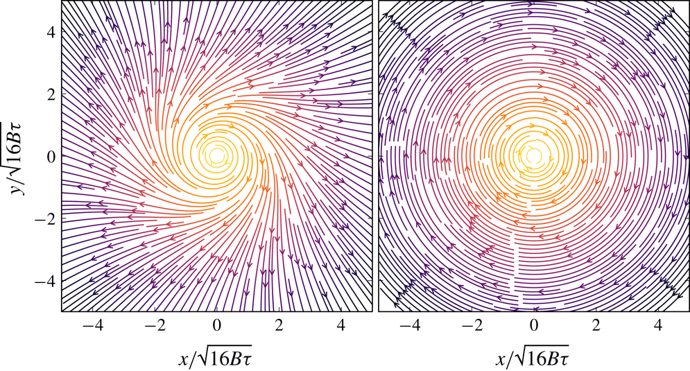
which is actually one of the two solutions obtained by Bai et al. (Reference Bai, Crumeyrolle and Mutabazi2015) (provided that one corrects the mistake in their computation). The field profiles are plotted in figure 3. Both fields tend to be azimuthal at small distances (large relaxation times): this is the limit analogous to the MHD with an azimuthal field. At smaller relaxation times, the radial contribution distorts the field lines of
 $\boldsymbol{B}^{(1)}$
. This distortion will deflect the oscillations of the dumbbells and destabilise the flow if the frequencies are too low to compensate the deflection.
Field lines of the viscoelastic fields
 $\boldsymbol{B}^{(1)}$
and
 $\boldsymbol{B}^{(2)}$
whose expressions are given by (3.18) in the most magnetic-like gauge. The colours display the intensity (dark is low, yellow is high).

This gauge looks suitable to probe the analogy between the VEI and the MRI since one may expect to get instability modes analogous to the axial MRI because of the axial field
 $\boldsymbol{B}^{(3)}$
, and also to the azimuthal MRI because of the azimuthal field
 $\boldsymbol{B}^{(2)}$
, plus some purely viscoelastic effects due to
 $\boldsymbol{B}^{(1)}$
. It has also the advantage of being quite simple since the dynamics is driven by only six components instead of nine. However, a drawback is that it is not general: the condition
 $B_{r}=0$
is not always relevant to identify a magnetic-like field because the divergence also has terms coming from the
 $\unicode[STIX]{x1D703}$
and
 $z$
dependences. One may therefore wonder if it is generically possible to find three angles
 $\unicode[STIX]{x1D703}$
,
 $\unicode[STIX]{x1D719}$
,
 $\unicode[STIX]{x1D713}$
such that at least one magnetic current vanishes,
 $$\begin{eqnarray}\boldsymbol{F}^{(3)}(\unicode[STIX]{x1D703},\unicode[STIX]{x1D719},\unicode[STIX]{x1D713})=0,\end{eqnarray}$$
which means, using the gauge transformation (3.9),
 $$\begin{eqnarray}\text{F}_{i3}\rightarrow (\unicode[STIX]{x1D641}\mathit{O})_{i3}+U_{i}\text{B}_{lm}\unicode[STIX]{x2202}_{l}\mathit{O}_{m3}=0.\end{eqnarray}$$
This would provide three constraints in the form of three nonlinear partial differential equations coupled to the two other viscoelastic fields and currents. These equations would be very complicated to solve.
The fields
 $\boldsymbol{B}^{(2)}$
and
 $\boldsymbol{B}^{(3)}$
of the most magnetic-like gauge given by (3.18) can therefore only be identified with true magnetic fields in the Taylor–Couette base flow. The trivial generalisation of the gauge condition (3.17) is the following:
 $$\begin{eqnarray}\boldsymbol{R}\propto \boldsymbol{e}_{x},\quad Z_{y}=0.\end{eqnarray}$$
It differs from the condition (3.17) because we do not have in general
 $\boldsymbol{R}\boldsymbol{\cdot }\boldsymbol{Z}=0$
; nevertheless, it is still possible to align
 $\boldsymbol{R}$
along
 $\boldsymbol{e}_{x}$
, and then rotate the plane perpendicular to
 $\boldsymbol{e}_{\boldsymbol{x}}$
in order to set
 $B_{z}^{(2)}=0$
(i.e.
 $Z_{y}=0$
). However, these conditions have no physical meaning in terms of vanishing charges or currents any more.
Besides being hardly generalisable, the most magnetic-like gauge lacks elegance because there is still the antisymmetric matrix
 $\unicode[STIX]{x1D63C}$
which remains undetermined, hiding three degrees of freedom which are constrained by the gauge in a non-straightforward way and without a clear physical interpretation.
3.4 ‘Symmetric’ gauge
A consequence of the eigenvalue decomposition theorem is that any symmetric positive semidefinite matrix can be written as the square of a symmetric matrix, so that the polymeric stress tensor can generically be decomposed as
 $$\begin{eqnarray}\unicode[STIX]{x1D64F}_{p}=\unicode[STIX]{x1D63D}^{2},\end{eqnarray}$$
with
 $\unicode[STIX]{x1D63D}$
a symmetric matrix. This provides a second choice of gauge: the requirement that the matrix
 $\unicode[STIX]{x1D63D}$
is symmetric gives three additional constraints to the decomposition (2.7). In terms of the geometrical construction described in § 3.1, this amounts to aligning the vector
 $\boldsymbol{Z}$
along the vector field
 $\boldsymbol{B}^{(3)}$
and then rotating the plane perpendicular to
 $\boldsymbol{B}^{(3)}$
in order to get
 $B_{\unicode[STIX]{x1D703}}^{(1)}=B_{r}^{(2)}$
. The symmetric decomposition (3.22) was actually done by Balci et al. (Reference Balci, Thomases, Renardy and Doering2011). They write the induction equation (2.8) and showed that the antisymmetric matrix
 $\unicode[STIX]{x1D63C}$
could be constrained. Indeed, writing the induction equation in matrix form,
 $$\begin{eqnarray}\unicode[STIX]{x2202}_{t}\unicode[STIX]{x1D63D}+\boldsymbol{U}\boldsymbol{\cdot }\unicode[STIX]{x1D735}\unicode[STIX]{x1D63D}-(\unicode[STIX]{x1D735}\boldsymbol{U})^{\text{T}}\unicode[STIX]{x1D63D}=-\frac{1}{2\unicode[STIX]{x1D70F}}(\unicode[STIX]{x1D63D}-B_{0}^{2}(\unicode[STIX]{x1D63C}+\unicode[STIX]{x1D644})\unicode[STIX]{x1D63E}),\end{eqnarray}$$
and subtracting its transpose, one gets
 $$\begin{eqnarray}\frac{B_{0}^{2}}{2\unicode[STIX]{x1D70F}}(\unicode[STIX]{x1D63C}\unicode[STIX]{x1D63E}+\unicode[STIX]{x1D63E}\unicode[STIX]{x1D63C})=\unicode[STIX]{x1D63D}(\unicode[STIX]{x1D735}\boldsymbol{U})-(\unicode[STIX]{x1D735}\boldsymbol{U})^{\text{T}}\unicode[STIX]{x1D63D},\end{eqnarray}$$
or, in other words, one infers that the matrix
 $B_{0}^{2}\unicode[STIX]{x1D63C}\unicode[STIX]{x1D63E}/(2\unicode[STIX]{x1D70F})-\unicode[STIX]{x1D63D}(\unicode[STIX]{x1D735}\boldsymbol{U})$
should be symmetric. This gives three equations which constrain the matrix
 $\unicode[STIX]{x1D63C}$
. Balci et al. (Reference Balci, Thomases, Renardy and Doering2011) take advantage of the symmetry of
 $\unicode[STIX]{x1D63D}$
to perform efficient direct numerical simulation, showing that the results were more accurate and stable.
Furthermore, an elastic energy density can be defined as the square of the Frobenius norm of the matrix
 $\unicode[STIX]{x1D63D}$
:
 $$\begin{eqnarray}\frac{1}{2}\Vert \unicode[STIX]{x1D63D}\Vert ^{2}=\frac{1}{2}\mathop{\sum }_{k=1}^{3}\Vert \boldsymbol{B}^{(k)}\Vert ^{2}=\frac{1}{2}\,\text{Tr}(\unicode[STIX]{x1D63D}^{\text{T}}\unicode[STIX]{x1D63D}),\end{eqnarray}$$
which is actually the trace of the polymeric stress tensor. Note that this norm is gauge-invariant. Taking the trace of the constitutive equation (2.2) gives
 $$\begin{eqnarray}\frac{1}{2}\unicode[STIX]{x2202}_{t}\Vert \unicode[STIX]{x1D63D}\Vert ^{2}+\frac{1}{2}\boldsymbol{U}\boldsymbol{\cdot }\unicode[STIX]{x1D735}\Vert \unicode[STIX]{x1D63D}\Vert ^{2}-\left(\mathop{\sum }_{k=1}^{3}\boldsymbol{B}^{(k)}\otimes \boldsymbol{B}^{(k)}\right)\boldsymbol{ : }\unicode[STIX]{x1D735}\boldsymbol{U}=-\frac{1}{2\unicode[STIX]{x1D70F}}(\Vert \unicode[STIX]{x1D63D}\Vert ^{2}-B_{0}^{2}),\end{eqnarray}$$
which is an equation for the conservation of the total viscoelastic energy. The first two terms on the left-hand side of (3.26) represent the total variation of the elastic potential energy density, and the third is a coupling term between the viscoelastic fields and the velocity gradient (i.e. the polymer stress on the velocity field), while the right-hand side gives the relaxation of the mechanical energy stored in the macromolecules during their interaction with the flow,
 $B_{0}^{2}$
being their minimal energy in the absence of the flow. The instabilities are driven by the transport of the elastic energy from the velocity to the fields: whenever a field gains some energy, it will store this energy while relaxing and, in the process, it will give part of its energy to the other fields and the velocity, leading to the destabilisation of the flow. If the relaxation time is very short, the fields will not have enough time to transfer their energy to the velocity and the destabilisation will not be efficient.
The coupling term
 $(\sum _{k=1}^{3}\boldsymbol{B}^{(k)}\otimes \boldsymbol{B}^{(k)})\boldsymbol{ : }\unicode[STIX]{x1D735}\boldsymbol{U}$
resembles the coupling term which appears in the conservation equation for the magnetic energy. However, it is not possible in the symmetric gauge to write three individual conservation equations. Another drawback is that the symmetry property lacks physical interpretation.
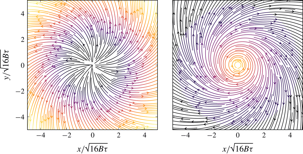
Field lines of the viscoelastic fields (a,c)
 $\boldsymbol{B}^{(1)}$
and (b,d)
 $\boldsymbol{B}^{(2)}$
, whose expressions are given by (3.27) in the symmetric gauge: (a,b) first solution, (c,d) second solution. The colours display the intensity (dark is low, yellow is high).

For the Taylor–Couette base flow, there are two different symmetric solutions:
 $$\begin{eqnarray}\unicode[STIX]{x1D63D}_{\pm }=\frac{B_{0}}{\sqrt{2}}\!\left(\begin{array}{@{}ccc@{}}\pm \left(1+\unicode[STIX]{x1D716}^{2}\pm \unicode[STIX]{x1D716}\sqrt{1+\unicode[STIX]{x1D716}^{2}}\right)^{-1/2} & \sqrt{1\pm {\displaystyle \frac{\unicode[STIX]{x1D716}}{\sqrt{1+\unicode[STIX]{x1D716}^{2}}}}} & 0\\ \sqrt{1\pm {\displaystyle \frac{\unicode[STIX]{x1D716}}{\sqrt{1+\unicode[STIX]{x1D716}^{2}}}}} & \sqrt{1\pm {\displaystyle \frac{\unicode[STIX]{x1D716}}{\sqrt{1+\unicode[STIX]{x1D716}^{2}}}}}\left(-{\displaystyle \frac{2}{\unicode[STIX]{x1D716}}}-\unicode[STIX]{x1D716}\pm \sqrt{1+\unicode[STIX]{x1D716}^{2}}\right) & 0\\ 0 & 0 & \sqrt{2}\end{array}\right)\!\!.\end{eqnarray}$$
The field profiles are plotted in figure 4. Note that the norm of
 $\boldsymbol{B}_{\pm }^{(1)}$
is always equal to
 $B_{0}/\sqrt{2}$
. The field
 $\boldsymbol{B}_{\pm }^{(2)}$
is azimuthal at large relaxation times (this is the limit analogous to the MHD). As in the most magnetic-like gauge, curvature effects appear at larger distances, either from the radial component of
 $\boldsymbol{B}_{+}^{(2)}$
for the first solution or from the one of
 $\boldsymbol{B}_{-}^{(1)}$
(second solution).
The associated charges and currents read
 $$\begin{eqnarray}{f_{0}}_{\pm }^{(1,2)}=\frac{B_{0}}{\sqrt{2}r}\unicode[STIX]{x1D709}_{\pm }^{(1,2)}(\unicode[STIX]{x1D716}),\quad {f_{0}}_{\pm }^{(3)}=0,\end{eqnarray}$$
 $$\begin{eqnarray}\boldsymbol{F}_{\pm }^{(1,2)}=\frac{B_{0}}{\sqrt{2}}\left(\frac{1}{2\unicode[STIX]{x1D70F}}\unicode[STIX]{x1D712}_{\pm }^{(1,2)}(\unicode[STIX]{x1D716})+\unicode[STIX]{x1D709}_{\pm }^{(1,2)}(\unicode[STIX]{x1D716})\frac{U_{\unicode[STIX]{x1D703}}}{r}\right)\boldsymbol{e}_{\unicode[STIX]{x1D703}},\quad \boldsymbol{F}_{\pm }^{(3)}=0,\end{eqnarray}$$
where the functions
 $\unicode[STIX]{x1D709}_{\pm }^{(1)}$
,
 $\unicode[STIX]{x1D709}_{\pm }^{(2)}$
,
 $\unicode[STIX]{x1D712}_{\pm }^{(1)}$
and
 $\unicode[STIX]{x1D712}_{\pm }^{(2)}$
are given in appendix D. Note that it is expected that the currents are azimuthal, and it should be the case in any gauge. Indeed, the application of any rotation on the right on the matrix current derived in the most magnetic-like gauge will only give azimuthal components to the three currents, and the remaining part of the gauge transformation (3.9) comes from the transformation of
 $f_{0}^{(k)}$
, which is multiplied by
 $\boldsymbol{U}$
and hence also provides azimuthal components.
The expressions obtained for the fields, charges and currents in the symmetric gauge are much more complicated than in the most magnetic-like gauge. This complexity is a consequence of the lack of physical interpretation of the symmetric gauge: while completely generalisable, it becomes hard to interpret the viscoelastic charges and currents obtained within the symmetry condition.
3.5 ‘Orthogonal’ gauge
Another possible choice of gauge is the gauge where the three viscoelastic fields are orthogonal. It is always possible to impose an orthogonality condition because
 $\unicode[STIX]{x1D63D}^{\text{T}}\unicode[STIX]{x1D63D}$
is a symmetric matrix so it has an eigenvalue decomposition in terms of a rotation matrix
 $\mathit{O}$
:
 $$\begin{eqnarray}\unicode[STIX]{x1D63D}^{\text{T}}\unicode[STIX]{x1D63D}=\mathit{O}\unicode[STIX]{x1D63F}\mathit{O}^{\text{T}}\quad \Longleftrightarrow \quad (\unicode[STIX]{x1D63D}\mathit{O})^{\text{T}}\unicode[STIX]{x1D63D}\mathit{O}=\unicode[STIX]{x1D63F},\end{eqnarray}$$
where
 $\unicode[STIX]{x1D63F}$
is a diagonal matrix. Thus one can fix the gauge by choosing the matrix
 $\unicode[STIX]{x1D63D}$
such that
 $\unicode[STIX]{x1D63D}^{\text{T}}\unicode[STIX]{x1D63D}=\unicode[STIX]{x1D63F}$
, which implies that the three fields
 $\{\boldsymbol{B}^{(k)}\}$
are orthogonal, and therefore constitute the primitive cell of an orthorhombic lattice. Thus the reciprocal vectors
 $\{\boldsymbol{C}^{(k)}\}$
are collinear to the original vectors
 $\{\boldsymbol{B}^{(k)}\}$
. The magnetic currents are therefore now expressed as
 $$\begin{eqnarray}\boldsymbol{F}^{(k)}=\frac{f_{0}^{(k)}}{\unicode[STIX]{x1D70F}}\boldsymbol{U}+\frac{1}{2\unicode[STIX]{x1D70F}}\left(\unicode[STIX]{x1D644}-\left(\frac{B_{0}}{\Vert \boldsymbol{B}^{(k)}\Vert }\right)^{2}\left(\unicode[STIX]{x1D63C}+\unicode[STIX]{x1D644}\right)\right)\boldsymbol{B}^{(k)}\end{eqnarray}$$
and the viscoelastic induction equation reads
 $$\begin{eqnarray}\unicode[STIX]{x2202}_{t}\boldsymbol{B}^{(k)}+(\boldsymbol{U}\boldsymbol{\cdot }\unicode[STIX]{x1D735})\boldsymbol{B}^{(k)}-\boldsymbol{B}^{(k)}\boldsymbol{\cdot }\unicode[STIX]{x1D735}\boldsymbol{U}=-\frac{1}{2\unicode[STIX]{x1D70F}}\left(\unicode[STIX]{x1D644}-\frac{B_{0}^{2}}{\Vert \boldsymbol{B}^{(k)}\Vert ^{2}}\left(\unicode[STIX]{x1D63C}+\unicode[STIX]{x1D644}\right)\right)\boldsymbol{B}^{(k)}.\end{eqnarray}$$
Multiplying it by
 $\boldsymbol{B}^{(k)}$
we get an induction equation for the norm (
 $\unicode[STIX]{x1D63C}$
being antisymmetric, the product
 $\unicode[STIX]{x1D63C}\boldsymbol{B}^{(k)}$
is orthogonal to
 $\boldsymbol{B}^{(k)}$
such that we get rid of
 $\unicode[STIX]{x1D63C}$
):
 $$\begin{eqnarray}\frac{1}{2}\unicode[STIX]{x2202}_{t}\Vert \boldsymbol{B}^{(k)}\Vert ^{2}+\frac{1}{2}(\boldsymbol{U}\boldsymbol{\cdot }\unicode[STIX]{x1D735})\Vert \boldsymbol{B}^{(k)}\Vert ^{2}-(\boldsymbol{B}^{(k)}\otimes \boldsymbol{B}^{(k)})\boldsymbol{ : }\unicode[STIX]{x1D735}\boldsymbol{U}=-\frac{1}{2\unicode[STIX]{x1D70F}}(\Vert \boldsymbol{B}^{(k)}\Vert ^{2}-B_{0}^{2}).\end{eqnarray}$$
This is actually the equation for the conservation of the elastic energy
 $\Vert \boldsymbol{B}^{(k)}\Vert ^{2}/2$
associated with the field
 $\boldsymbol{B}^{(k)}$
, the sum of these individual elastic energies being precisely the total elastic energy defined by (3.25). Summing equation (3.33) with the equation of conservation of the flow kinetic energy provides an equation for the individual contribution of the field
 $\boldsymbol{B}^{(k)}$
to the total energy density:
 $$\begin{eqnarray}\displaystyle (\unicode[STIX]{x2202}_{t}+\boldsymbol{U}\boldsymbol{\cdot }\unicode[STIX]{x1D735}){\mathcal{E}} & = & \displaystyle \mathop{\sum }_{k=1}^{3}\unicode[STIX]{x1D735}\boldsymbol{\cdot }((\boldsymbol{B}^{(k)}\boldsymbol{\cdot }\boldsymbol{U})\boldsymbol{B}^{(k)})-\boldsymbol{U}\boldsymbol{\cdot }\unicode[STIX]{x1D735}\unicode[STIX]{x1D6F9}_{p}-\mathop{\sum }_{k=1}^{3}\frac{1}{2\unicode[STIX]{x1D70F}}(\Vert \boldsymbol{B}^{(k)}\Vert ^{2}-B_{0}^{2})\nonumber\\ \displaystyle & & \displaystyle +\,\unicode[STIX]{x1D70C}\unicode[STIX]{x1D708}_{s}\boldsymbol{U}\boldsymbol{\cdot }\unicode[STIX]{x1D6FB}^{2}\boldsymbol{U},\end{eqnarray}$$
where the quantity
 $$\begin{eqnarray}{\mathcal{E}}=\unicode[STIX]{x1D70C}\frac{\Vert \boldsymbol{U}\Vert ^{2}}{2}+\mathop{\sum }_{k=1}^{3}\frac{\Vert \boldsymbol{B}^{(k)}\Vert ^{2}}{2}\end{eqnarray}$$
represents the total energy density of the viscoelastic flow: it consists of the fluid kinetic energy and the polymer elastic energy.
Equation (3.34) is a generalisation of the one obtained by Fouxon & Lebedev (Reference Fouxon and Lebedev2003) in the limit of infinite relaxation time (assuming that there is a single solenoidal field
 $\boldsymbol{B}$
with vanishing minimal elastic energy). The rate of variation of the energy of a viscoelastic flow is due to the transfer between the viscoelastic field and the flow field (through the polymer stresses on the fluid), to the relaxation of energy stored by viscoelastic field and to viscous dissipation. In the dynamic equilibrium conditions, the energy interaction between polymer stresses and the fluid is balanced by the relaxation of viscoelastic field energy and the viscous dissipation.
The equation for the conservation of the total energy (3.34) is gauge-invariant, while the equation for the individual elastic energies (3.33) is only valid in the orthogonal gauge. In the orthogonal gauge, the coupling term is more meaningful than in the symmetric gauge and it can be directly compared with the one appearing in the conservation of the magnetic energy. Each viscoelastic field, while relaxing, gives part of its energy to the velocity (and not directly to the other fields). The coupling between the three viscoelastic fields induces volumetric deformations, a feature that is not taken into account when considering only the transfers of the total energy (Hameduddin et al. Reference Hameduddin, Meneveau, Zaki and Gayme2018).
Finally, we show in appendix E that an expression for
 $\unicode[STIX]{x1D63C}\boldsymbol{B}^{(k)}$
can be obtained so that the matrix
 $\unicode[STIX]{x1D63C}$
is removed from the viscoelastic currents:
 $$\begin{eqnarray}\left.\begin{array}{@{}c@{}}\unicode[STIX]{x1D63C}\boldsymbol{B}^{(k)}=-2\unicode[STIX]{x1D70F}\left({\displaystyle \frac{\Vert \boldsymbol{B}^{(k)}\Vert }{B_{0}}}\right)^{2}\displaystyle \mathop{\sum }_{\substack{ \unicode[STIX]{x1D706}=1 \\ \unicode[STIX]{x1D706}\neq k}}^{3}{\displaystyle \frac{\boldsymbol{B}^{(\unicode[STIX]{x1D706})}\otimes \boldsymbol{B}^{(\unicode[STIX]{x1D706})}}{\Vert \boldsymbol{B}^{(\unicode[STIX]{x1D706})}\Vert ^{2}-\Vert \boldsymbol{B}^{(k)}\Vert ^{2}}}(\unicode[STIX]{x1D735}\boldsymbol{U}+\unicode[STIX]{x1D735}\boldsymbol{U}^{\text{T}})\boldsymbol{B}^{(k)},\\ \boldsymbol{F}^{(k)}={\displaystyle \frac{f_{0}^{(k)}}{\unicode[STIX]{x1D70F}}}\boldsymbol{U}+{\displaystyle \frac{\Vert \boldsymbol{B}^{(k)}\Vert ^{2}-B_{0}^{2}}{2\unicode[STIX]{x1D70F}\Vert \boldsymbol{B}^{(k)}\Vert ^{2}}}\boldsymbol{B}^{(k)}+\displaystyle \mathop{\sum }_{\substack{ \unicode[STIX]{x1D706}=1 \\ \unicode[STIX]{x1D706}\neq k}}^{3}{\displaystyle \frac{\boldsymbol{B}^{(\unicode[STIX]{x1D706})}\otimes \boldsymbol{B}^{(\unicode[STIX]{x1D706})}}{\Vert \boldsymbol{B}^{(\unicode[STIX]{x1D706})}\Vert ^{2}-\Vert \boldsymbol{B}^{(k)}\Vert ^{2}}}(\unicode[STIX]{x1D735}\boldsymbol{U}+\unicode[STIX]{x1D735}\boldsymbol{U}^{\text{T}})\boldsymbol{B}^{(k)}.\end{array}\right\}\end{eqnarray}$$
Note that, for all
 $k\neq \unicode[STIX]{x1D706}$
,
 $\Vert \boldsymbol{B}^{(\unicode[STIX]{x1D706})}\Vert ^{2}=\Vert \boldsymbol{B}^{(k)}\Vert ^{2}~\Longrightarrow ~\boldsymbol{B}^{(\unicode[STIX]{x1D706})}\otimes \boldsymbol{B}^{(\unicode[STIX]{x1D706})}(\unicode[STIX]{x1D735}\boldsymbol{U}+\unicode[STIX]{x1D735}\boldsymbol{U}^{\text{T}})\boldsymbol{B}^{(k)}=0$
(as shown in appendix F), so that there is no singularity. The physical meaning of the matrix
 $\unicode[STIX]{x1D63C}$
becomes clear in (3.36): it is the coupling of the viscoelastic currents, which causes the deflection of the viscoelastic charges. In the orthogonal gauge, it affects only the direction of the fields and not their energy.
One may wonder why this coupling does not seem to vanish in the limit
 $\unicode[STIX]{x1D70F}\rightarrow \infty$
. This is due to the degeneracy of the asymptotic matrix
 $\unicode[STIX]{x1D63D}$
, which should be of the same rank as the polymeric stress tensor, i.e. of rank 1, while (3.36) is derived assuming a non-degenerate matrix
 $\unicode[STIX]{x1D63D}$
. This means in general that either the three viscoelastic fields are equal, or two are equal and one vanishes, or two vanish; and in the orthogonal gauge the only possibility is that two fields vanish, hence the coupling
 $\unicode[STIX]{x1D63C}\boldsymbol{B}^{(k)}$
should be zero. This is consistent with the induction equation that one obtains when two fields vanish. In this case, one cannot follow the derivation given in appendix A because the matrix
 $\unicode[STIX]{x1D63E}$
does not exist, and the induction equation for the non-vanishing field reads, in components,
 $$\begin{eqnarray}B_{i}{\mathcal{I}}_{j}=\text{A}_{ij},\quad {\mathcal{I}}_{j}\equiv [\unicode[STIX]{x2202}_{t}B_{j}+(\boldsymbol{U}\boldsymbol{\cdot }\unicode[STIX]{x1D735})B_{j}-(\boldsymbol{B}\boldsymbol{\cdot }\unicode[STIX]{x1D735})U_{j}],\end{eqnarray}$$
which implies that
 $$\begin{eqnarray}\left.\begin{array}{@{}rcl@{}}\forall i,\quad B_{i}{\mathcal{I}}_{i}=0\, & \quad \Longrightarrow \, & \quad \forall i,\quad B_{i}=0\quad \text{or}\quad {\mathcal{I}}_{i}=0\\ \, & \quad \Longrightarrow \, & \quad \forall i,\forall j,\quad \text{A}_{ij}=0\quad \text{or}\quad \forall j,\quad \text{A}_{ji}=0,\\ \, & \quad \Longrightarrow \, & \quad \forall i,\forall j,\quad \text{A}_{ij}=0,\end{array}\right\}\end{eqnarray}$$
hence
 $\unicode[STIX]{x1D63C}=0$
(which is consistent with the fact that we recover the induction equation of the MHD in the limit
 $\unicode[STIX]{x1D70F}^{-1}=\unicode[STIX]{x1D702}=0$
, which is actually not so trivial!).
In conclusion, equation (3.36) is consistent even in the limit
 $\unicode[STIX]{x1D70F}\rightarrow \infty$
where the degeneracy of
 $\unicode[STIX]{x1D63D}$
may raise some issues. Furthermore, we see that the requirement of having equal non-vanishing fields in this limit will always be fulfilled and actually in a better way than in the most magnetic-like gauge, because in the orthogonal gauge there will be only one field left. From the point of view of electromagnetism, two copies of the MHD vanish so that there is only one set of Maxwell’s equations left.
The orthogonal gauge, in which we are able to write the viscoelastic currents without
 $\unicode[STIX]{x1D63C}$
, is therefore more elegant than the previous gauges: it is fully general and the orthogonality of the three viscoelastic fields makes them intuitive to visualise, while individual energy conservation equations can be written. However, the price to pay is a more complicated gauge-fixing condition since the orthogonality conditions are nonlinear and the three fields contain nine degrees of freedom instead of only six in the previous gauges.
Field lines of the viscoelastic fields
 $\boldsymbol{B}^{(1)}$
and
 $\boldsymbol{B}^{(2)}$
whose expressions are given by (3.41). The colours display the intensity (dark is low, yellow is high). For readability purposes, these two colour maps are not calibrated in the same way.

The viscoelastic Maxwell’s equations (2.11) with the viscoelastic currents (3.31) can be solved for the Taylor–Couette base flow. As shown in § 2.5 the matrix
 $\unicode[STIX]{x1D63C}$
is invariant under the gauge rotation, so (2.21) holds in the orthogonal gauge and the viscoelastic Maxwell’s equations give
 $$\begin{eqnarray}\left.\begin{array}{@{}c@{}}B_{r}^{(k)}=\left({\displaystyle \frac{B_{0}}{\Vert \boldsymbol{B}^{(k)}\Vert }}\right)^{2}\left(-{\displaystyle \frac{1}{\unicode[STIX]{x1D716}}}B_{\unicode[STIX]{x1D703}}^{(k)}+B_{r}^{(k)}\right),\\ {\displaystyle \frac{2}{\unicode[STIX]{x1D716}}}B_{r}^{(k)}+B_{\unicode[STIX]{x1D703}}^{(k)}=\left({\displaystyle \frac{B_{0}}{\Vert \boldsymbol{B}^{(k)}\Vert }}\right)^{2}\left({\displaystyle \frac{1}{\unicode[STIX]{x1D716}}}B_{r}^{(k)}+B_{\unicode[STIX]{x1D703}}^{(k)}\right),\\ B_{z}^{(k)}\left(1-\left({\displaystyle \frac{B_{0}}{\Vert \boldsymbol{B}^{(k)}\Vert }}\right)^{2}\right)=0,\end{array}\right\}\end{eqnarray}$$
which implies that either
 $\Vert \boldsymbol{B}^{(k)}\Vert =B_{0}$
or
 $B_{z}^{(k)}=0$
. In the former case, the first two equations give
 $B_{r}^{(k)}=B_{\unicode[STIX]{x1D703}}^{(k)}=0$
so that the field
 $\boldsymbol{B}^{(k)}=B_{0}\boldsymbol{e}_{z}$
is a solution of the viscoelastic Maxwell’s equations in the orthogonal gauge. In the latter case we get
 $$\begin{eqnarray}B_{r}^{(k)}=\frac{B_{0}}{\sqrt{2}},\quad B_{\unicode[STIX]{x1D703}}^{(k)}=\frac{B_{0}}{\sqrt{2}}\left(-\frac{1}{\unicode[STIX]{x1D716}}\pm \sqrt{1+\frac{1}{\unicode[STIX]{x1D716}^{2}}}\right).\end{eqnarray}$$
The orthogonality condition
 $\unicode[STIX]{x1D63D}^{\text{T}}\unicode[STIX]{x1D63D}=\unicode[STIX]{x1D63F}$
therefore completely fixes the gauge and leads to a solution similar to that found in Cartesian coordinates by Ogilvie & Proctor (Reference Ogilvie and Proctor2003):
 $$\begin{eqnarray}\unicode[STIX]{x1D63D}=\frac{B_{0}}{\sqrt{2}}\left(\begin{array}{@{}ccc@{}}1 & 1 & 0\\ -{\displaystyle \frac{1}{\unicode[STIX]{x1D716}}}+\sqrt{1+{\displaystyle \frac{1}{\unicode[STIX]{x1D716}^{2}}}} & -{\displaystyle \frac{1}{\unicode[STIX]{x1D716}}}-\sqrt{1+{\displaystyle \frac{1}{\unicode[STIX]{x1D716}^{2}}}} & 0\\ 0 & 0 & \sqrt{2}\end{array}\right).\end{eqnarray}$$
Note that
 $B_{r}^{3}=0$
so that the field
 $\boldsymbol{B}^{(3)}$
can be interpreted as an axial magnetic field, while the other two fields will be responsible for purely viscoelastic instabilities. Note also that two fields vanish in the limit
 $\unicode[STIX]{x1D70F}\rightarrow \infty$
, as expected.
The field lines of the two viscoelastic fields
 $\boldsymbol{B}^{(1)}$
and
 $\boldsymbol{B}^{(2)}$
are plotted in figure 5. The field
 $\boldsymbol{B}^{(1)}$
tends to be radial with a small intensity at large relaxation times and curvature effects appear at large distances (small relaxation time). On the contrary, the field
 $\boldsymbol{B}^{(2)}$
is azimuthal at large relaxation time: this is the limit analogous to the MHD. As in the previous gauges, radial distortion appears at small relaxation times and will deflect the oscillations of the dumbbells. In the orthogonal gauge, the three viscoelastic fields will describe the oscillation of a particle fluid under a strain applied in three orthogonal directions.
The viscoelastic charges and currents associated with the orthogonal viscoelastic fields given by (3.41) are very similar to the ones obtained in the most magnetic-like gauge and read
 $$\begin{eqnarray}\left.\begin{array}{@{}c@{}}{\displaystyle \frac{f_{0}^{(1)}}{\unicode[STIX]{x1D70F}}}={\displaystyle \frac{f_{0}^{(2)}}{\unicode[STIX]{x1D70F}}}={\displaystyle \frac{B_{0}}{\sqrt{2}r}},\quad f_{0}^{(3)}=0,\\ \boldsymbol{F}^{(1)}=\boldsymbol{F}^{(2)}={\displaystyle \frac{B_{0}}{\sqrt{2}}}(\unicode[STIX]{x2202}_{r}U_{\unicode[STIX]{x1D703}})\boldsymbol{e}_{\unicode[STIX]{x1D703}},\quad \boldsymbol{F}^{(3)}=0.\end{array}\right\}\end{eqnarray}$$
The orthogonal gauge is more physically interpretable than the symmetric gauge, and it is more generalisable than the most magnetic-like gauge. However, its drawback is that the gauge-fixing condition (the requirement that the three viscoelastic fields are orthogonal) is nonlinear. Table 1 summarises the advantages and drawbacks found for the three previously studied gauges.
Comparison between the three gauges studied in the present work (GFC means ‘gauge-fixing condition’ and T–C means ‘Taylor–Couette’).

4 Stability analysis
Having achieved the formulation of the Oldroyd-B model in terms of viscoelastic fields, we now investigate the stability of the Taylor–Couette flow in order to find which fields have a key contribution to the destabilisation.
4.1 Dimensionless equations
To get dimensionless quantities, we use the following scalings:
 $$\begin{eqnarray}\left.\begin{array}{@{}c@{}}r\rightarrow rd,\quad t\rightarrow t/\dot{\unicode[STIX]{x1D6FE}},\quad \dot{\unicode[STIX]{x1D6FE}}=|\unicode[STIX]{x1D6FA}_{i}a-\unicode[STIX]{x1D6FA}_{o}b|/(b-a),\\ \unicode[STIX]{x1D64F}_{p}\rightarrow (\unicode[STIX]{x1D70C}\dot{\unicode[STIX]{x1D6FE}}\unicode[STIX]{x1D708})\unicode[STIX]{x1D64F}_{p},\quad \boldsymbol{U}\rightarrow |\unicode[STIX]{x1D6FA}_{i}a-\unicode[STIX]{x1D6FA}_{o}b|\boldsymbol{U},\quad \unicode[STIX]{x1D6F9}\rightarrow (\unicode[STIX]{x1D70C}\dot{\unicode[STIX]{x1D6FE}}\unicode[STIX]{x1D708})\unicode[STIX]{x1D6F9},\\ \boldsymbol{B}^{(k)}\rightarrow \sqrt{\unicode[STIX]{x1D707}_{0}\unicode[STIX]{x1D70C}\dot{\unicode[STIX]{x1D6FE}}\unicode[STIX]{x1D708}}\boldsymbol{B}^{(k)},\quad \boldsymbol{E}^{(k)}\rightarrow \sqrt{\unicode[STIX]{x1D707}_{0}\unicode[STIX]{x1D70C}\dot{\unicode[STIX]{x1D6FE}}\unicode[STIX]{x1D708}}(b-a)\dot{\unicode[STIX]{x1D6FE}}\boldsymbol{E}^{(k)},\\ f_{0}^{(k)}\rightarrow {\displaystyle \frac{\sqrt{\unicode[STIX]{x1D707}_{0}\unicode[STIX]{x1D70C}\dot{\unicode[STIX]{x1D6FE}}\unicode[STIX]{x1D708}}}{\dot{\unicode[STIX]{x1D6FE}}(b-a)}}f_{0}^{(k)},\quad \boldsymbol{F}^{(k)}\rightarrow \sqrt{\unicode[STIX]{x1D707}_{0}\unicode[STIX]{x1D70C}\dot{\unicode[STIX]{x1D6FE}}^{3}\unicode[STIX]{x1D708}}\boldsymbol{F}^{(k)},\end{array}\right\}\end{eqnarray}$$
where
 $\unicode[STIX]{x1D708}=\unicode[STIX]{x1D708}_{s}+\unicode[STIX]{x1D708}_{p}$
is the total viscosity of the viscoelastic fluid. The dimensionless viscoelastic Maxwell’s equations read
 $$\begin{eqnarray}\displaystyle \left.\begin{array}{@{}c@{}}\unicode[STIX]{x1D735}\boldsymbol{\cdot }\boldsymbol{B}={\displaystyle \frac{f_{0}}{Wi}},\\ \unicode[STIX]{x1D735}\times \boldsymbol{ E}=-\unicode[STIX]{x2202}_{t}\boldsymbol{B}-\boldsymbol{F},\\ \boldsymbol{ E}+\boldsymbol{ U}\times \boldsymbol{ B}=0,\\ \boldsymbol{F}={\displaystyle \frac{1}{2Wi}}\left(\boldsymbol{B}+2f_{0}\boldsymbol{U}-{\displaystyle \frac{S}{Wi}}(\unicode[STIX]{x1D63C}+\unicode[STIX]{x1D644})\boldsymbol{C}\right),\end{array}\right\} & & \displaystyle\end{eqnarray}$$
where
 $Wi=\unicode[STIX]{x1D70F}\dot{\unicode[STIX]{x1D6FE}}$
is the Weissenberg number and
 $S=\unicode[STIX]{x1D708}_{p}/\unicode[STIX]{x1D708}$
is the viscosity ratio. The dimensionless Navier–Stokes equation and the incompressibility condition read
 $$\begin{eqnarray}\left.\begin{array}{@{}c@{}}Re(\unicode[STIX]{x2202}_{t}\boldsymbol{U}+\boldsymbol{U}\boldsymbol{\cdot }\unicode[STIX]{x1D735}\boldsymbol{U})=-\unicode[STIX]{x1D735}\unicode[STIX]{x1D6F9}+\displaystyle \mathop{\sum }_{k=1}^{3}((\unicode[STIX]{x1D735}\boldsymbol{\cdot }\boldsymbol{B}^{(k)})\boldsymbol{B}^{(k)}+\boldsymbol{B}^{(k)}\boldsymbol{\cdot }\unicode[STIX]{x1D735}\boldsymbol{B}^{(k)})+(1-S)\unicode[STIX]{x1D6FB}^{2}\boldsymbol{U},\\ \unicode[STIX]{x1D735}\boldsymbol{\cdot }\boldsymbol{U}=0,\end{array}\right\}\end{eqnarray}$$
where
 $Re=b^{2}\unicode[STIX]{x1D6FA}_{i}(1-\unicode[STIX]{x1D702})|\unicode[STIX]{x1D702}-\unicode[STIX]{x1D707}|/\unicode[STIX]{x1D708}$
is the shear Reynolds number. Thus there are three independent parameters to describe the dynamics of the viscoelastic flow:
 $Re$
,
 $Wi$
and
 $S$
.
4.2 Numerical procedure
In a given gauge, we consider small perturbations around the base flow:
 $$\begin{eqnarray}\boldsymbol{X}=\boldsymbol{X}^{0}+\unicode[STIX]{x1D739}\boldsymbol{X}(r)\text{e}^{st+\text{i}(m\unicode[STIX]{x1D703}+qz)},\end{eqnarray}$$
where
 $s=\unicode[STIX]{x1D70E}+\text{i}\unicode[STIX]{x1D714}$
,
 $\unicode[STIX]{x1D70E}$
is the growth rate,
 $\unicode[STIX]{x1D714}$
the angular frequency,
 $m\in \mathbb{N}$
the azimuthal wavenumber and
 $q\in \mathbb{R}$
the axial wavenumber. The symbol
 $\boldsymbol{X}$
represents the fields
 $\boldsymbol{B}^{(k)}$
, the corresponding fields
 $\boldsymbol{E}^{(k)}$
, the velocity
 $\boldsymbol{U}$
and the pressure
 $\unicode[STIX]{x1D6F9}$
.
An important remark is that the gauge invariance holds on the total field and not on the individual contributions from the base flow and the perturbation. This means that the gauge for the perturbation should be fixed using the same conditions as the ones fixing the unperturbed field.
As discussed in § 3.3, in the most magnetic-like gauge we do not have in general
 $\boldsymbol{R}\boldsymbol{\cdot }\boldsymbol{Z}=0$
(where
 $\boldsymbol{R}$
and
 $\boldsymbol{Z}$
are defined by (3.3a–c
)). We therefore fix the gauge using the trivial (but meaningless) generalisation (3.21a,b
). In matrix form, the dimensionless perturbed magnetic fields in this gauge read
 $$\begin{eqnarray}\unicode[STIX]{x1D63D}=B_{0}\left(\begin{array}{@{}ccc@{}}1 & 0 & 0\\ -{\displaystyle \frac{1}{\unicode[STIX]{x1D716}}} & -{\displaystyle \frac{1}{\unicode[STIX]{x1D716}}}\sqrt{1+\unicode[STIX]{x1D716}^{2}} & 0\\ 0 & 0 & 1\end{array}\right)+B_{0}\left(\begin{array}{@{}ccc@{}}\unicode[STIX]{x1D6FF}r_{1}(r) & 0 & 0\\ \unicode[STIX]{x1D6FF}t_{1}(r) & \unicode[STIX]{x1D6FF}t_{2}(r) & \unicode[STIX]{x1D6FF}t_{3}(r)\\ \unicode[STIX]{x1D6FF}z_{1}(r) & 0 & \unicode[STIX]{x1D6FF}z_{3}(r)\end{array}\right)\text{e}^{st+\text{i}(m\unicode[STIX]{x1D703}+qz)},\end{eqnarray}$$
where
 $B_{0}=\sqrt{S/Wi}$
,
 $\unicode[STIX]{x1D716}=2KWi/r^{2}$
and
 $K=(1-\unicode[STIX]{x1D707})\unicode[STIX]{x1D702}^{2}/[(1-\unicode[STIX]{x1D702}^{2})/(1-\unicode[STIX]{x1D702})/(\unicode[STIX]{x1D702}-\unicode[STIX]{x1D707})]$
. There are only six perturbed quantities, while the viscoelastic Maxwell’s equations (4.2) provide nine constraints. The three missing unknowns are hidden in the antisymmetric matrix
 $\unicode[STIX]{x1D63C}$
, which should also be perturbed:
 $$\begin{eqnarray}\unicode[STIX]{x1D63C}=\unicode[STIX]{x1D63C}^{0}+\unicode[STIX]{x1D6FF}\unicode[STIX]{x1D63C}(r)\text{e}^{st+\text{i}(m\unicode[STIX]{x1D703}+qz)}\end{eqnarray}$$
in order to have a well-defined problem.
In the case of the symmetric gauge, the generalisation is straightforward and the dimensionless perturbed magnetic fields read
 $$\begin{eqnarray}\unicode[STIX]{x1D6FF}\unicode[STIX]{x1D63D}=B_{0}\left(\begin{array}{@{}ccc@{}}\unicode[STIX]{x1D6FF}r_{1}(r) & \unicode[STIX]{x1D6FF}t_{1}(r) & \unicode[STIX]{x1D6FF}z_{1}(r)\\ \unicode[STIX]{x1D6FF}t_{1}(r) & \unicode[STIX]{x1D6FF}t_{2}(r) & \unicode[STIX]{x1D6FF}z_{2}(r)\\ \unicode[STIX]{x1D6FF}z_{1}(r) & \unicode[STIX]{x1D6FF}z_{2}(r) & \unicode[STIX]{x1D6FF}z_{3}(r)\end{array}\right)\text{e}^{st+\text{i}(m\unicode[STIX]{x1D703}+qz)}\end{eqnarray}$$
and the matrix
 $\unicode[STIX]{x1D63C}$
is also perturbed.
In the case of the orthogonal gauge, we use the expression (3.36) in order to get rid of the matrix
 $\unicode[STIX]{x1D63C}$
, such that we have nine perturbed components in the magnetic fields as unknowns and nine Maxwell’s equations.
In either gauge, the system of linearised equations can be put in matrix form as follows:
 $$\begin{eqnarray}\unicode[STIX]{x1D6EC}(m,q)\unicode[STIX]{x1D739}\boldsymbol{X}=s\unicode[STIX]{x1D648}\unicode[STIX]{x1D739}\boldsymbol{X},\end{eqnarray}$$
where
 $\unicode[STIX]{x1D6EC}$
is a differential operator,
 $\unicode[STIX]{x1D648}$
a diagonal matrix and
 $\unicode[STIX]{x1D739}\boldsymbol{X}$
a vector containing the 10 perturbed quantities. The stability analysis amounts to finding, for a given set of control parameters
 $(Re,Wi,S)$
, the eigenvalue of the operator
 $\unicode[STIX]{x1D6EC}$
having the largest real part and optimised with respect to
 $m$
and
 $q$
. This was solved using the Mathematica package Eigen (see http://library.wolfram.com/infocenter/MathSource/8762/), which makes use of the Chebyshev collocation method to discretise the differential operator on a mesh lattice. After several tests it appeared that only 30 Chebyshev polynomials were sufficient to get reliable results while substantially decreasing the computation time.
4.3 Results
To validate our decomposition of the polymeric stress tensor into viscoelastic fields, we have computed the map of the optimised growth rate
 $\unicode[STIX]{x1D70E}=f(Wi,Re)$
at
 $S=0.5$
and
 $\unicode[STIX]{x1D702}=0.95$
in the Keplerian regime in the three gauges. The results computed in any gauge were identical and are plotted in figure 6(a). This stability diagram matches the ones computed by Ogilvie & Potter (Reference Ogilvie and Potter2008) and Bai (Reference Bai2015). We retrieved as expected the same results since the constitutive tensor equation of the Oldroyd-B model is completely equivalent to our viscoelastic Maxwell’s equations in either gauge.
One of the advantages of the formulation in terms of viscoelastic fields is that it allows one to compare the individual contributions of each field. To this end, we recomputed in the orthogonal gauge the stability diagram
 $\unicode[STIX]{x1D70E}=f(Wi,Re)$
for
 $S=0.5$
and
 $\unicode[STIX]{x1D702}=0.95$
in the Keplerian regime for each viscoelastic field separately, i.e. we perturbed one field at a time, putting the other perturbations to zero, and keeping the critical wavenumbers obtained in the general case. The fields
 $\boldsymbol{B}^{(1)}$
and
 $\boldsymbol{B}^{(3)}$
were found to induce no instability in the parameter space under investigation, so only the field
 $\boldsymbol{B}^{(2)}$
is responsible for the flow destabilisation. The result for the effect of
 $\boldsymbol{B}^{(2)}$
is shown in figure 6(b).
Optimised growth rate
 $\unicode[STIX]{x1D70E}=f(Wi,Re)$
at
 $S=0.5$
and
 $\unicode[STIX]{x1D702}=0.95$
in the Keplerian regime: comparison between (a) the general analysis, and (b) the result where only the perturbations on
 $\boldsymbol{B}^{(2)}$
are taken into account in the orthogonal gauge. In order to match the normalisation defined by Ogilvie & Potter (Reference Ogilvie and Potter2008),
 $Re$
and
 $Wi$
defined in (4.2) are multiplied by
 $(\unicode[STIX]{x1D707}-1)\unicode[STIX]{x1D702}/(\unicode[STIX]{x1D707}-\unicode[STIX]{x1D702})$
and the growth rate by
 $(\unicode[STIX]{x1D702}-\unicode[STIX]{x1D707})/(1-\unicode[STIX]{x1D702})$
.

In this example, only the field
 $\boldsymbol{B}^{(2)}$
has a non-negligible contribution: its stability diagram is very similar to the one taking the three fields. This can be understood by noticing that, already at
 $Wi=1$
, the norm of
 $\boldsymbol{B}^{(2)}$
is more than 10 times bigger than the norm of
 $\boldsymbol{B}^{(3)}$
, and almost 30 times bigger than the norm of
 $\boldsymbol{B}^{(1)}$
, while at
 $Wi=10$
the ratios are bigger than 1000, and even 10 000 for
 $Wi>25$
. Importantly, this suggests that
 $\boldsymbol{B}^{(1)}$
and
 $\boldsymbol{B}^{(3)}$
may be ignored in order to get very good approximations of the marginal curves and stability diagrams. Of course, solving the equations involving only
 $\boldsymbol{B}^{(2)}$
is much simpler than solving the general ones, and this represents an important gain of computational efficiency.
Ogilvie & Potter (Reference Ogilvie and Potter2008) observed that the unstable parameter space at large
 $Re$
and
 $Wi$
is analogous to the azimuthal MRI. What we can conclude from the present analysis is that the whole parameter space should actually be identified with the effect of an azimuthal viscoelastic field. However, at small
 $Wi$
, this field cannot be identified with a magnetic field because of the presence of the viscoelastic currents inducing the deflection of the viscoelastic charges. These charges might be responsible for the instability obtained at small
 $Wi$
and large
 $Re$
both in experiments and in linear stability analysis (Bai et al.
Reference Bai, Crumeyrolle and Mutabazi2015). This instability manifests itself in the form of stationary vortices with a size smaller than the gap width. It cannot be identified with the axial MRI which would be induced by the axial magnetic-like field
 $\boldsymbol{B}^{(3)}$
, the contribution of the latter being too weak. The misleading interpretation of Bai et al. (Reference Bai, Crumeyrolle and Mutabazi2015), who identified a critical Weissenberg number
 $Wi_{c}$
below which the axial field
 $\boldsymbol{B}^{(3)}$
was predominant and could induce a regime analogous to the axial MRI, was due to a mistake in the computation of
 $\boldsymbol{B}^{(2)}$
. It is clear from (3.18) that the norm of
 $\boldsymbol{B}^{(2)}$
is always bigger than the one of
 $\boldsymbol{B}^{(3)}$
, so that it is not possible to define
 $Wi_{c}$
. The role of viscoelastic charges and currents in the destabilisation of viscoelastic flows becomes an open issue that needs to be clarified in forthcoming studies in Taylor–Couette flows and in other flow configurations of viscoelastic fluids.
5 Discussion and conclusion
We have investigated the analogy between viscoelastic hydrodynamic equations with the Oldroyd-B model and the MHD equations. The analogy has been extended to polymer solutions with finite relaxation time or conducting liquids with finite magnetic diffusivity. The results lead to those obtained in previous studies (Ogilvie & Potter Reference Ogilvie and Potter2008; Bai et al. Reference Bai, Crumeyrolle and Mutabazi2015) in the limit of infinite relaxation time of polymer solution and zero magnetic diffusivity of conducting liquids. We shed light on some inconsistencies of these studies by extending the analogy at the level of the Maxwell’s equations. We have identified the origin of the relaxation terms of the Oldroyd-B model as a result of viscoelastic currents analogous to magnetic currents, and we have set a framework to rigorously extend the analogy at finite relaxation times. We unveiled the existence of viscoelastic charges (analogue of magnetic monopoles) associated with the viscoelastic currents, and proposed an interpretation in terms of distributions of oscillations of damped elastic dumbbells.
One of the questions that may arise concerns the existence of any connection between polymer relaxation and diffusion. The relaxation of viscoelastic fluids comes from the relaxation of the fluid elements which can be microscopically viewed as small springs (dumbbell model of Kuhn and Peterlin). They store the elastic energy of the fluid until they get excited. For dilute solution, the polymer molecules diffuse in the solvent due to Brownian motion so that their diffusion coefficient is related to the relaxation time by
 $D=R_{g}^{2}/\unicode[STIX]{x1D70F}$
, where
 $R_{g}$
is the gyration radius of the molecule (Doi Reference Doi1986). In MHD, charge-carrying particles are tied strongly to magnetic field lines. Diffusion allows field lines to slip through the fluid. But, in reality, particles are random walking off one field line to another. So the two systems share the randomness of the charge carriers (polymer chains in viscoelastic solutions and charged particles in MHD). Equations (2.2) show that, if the nonlinear terms are neglected, the polymer stress tensor relaxes while the Maxwell stress tensor is diffusive. This connection needs to be investigated in more detail using either a Lagrangian formalism (Ogilvie Reference Ogilvie2016) or any statistical approach of diffusion processes (Bakunin Reference Bakunin2008).
The viscoelastic Maxwell’s equations have a fundamental gauge symmetry. We studied three gauges: two general gauges and one particular to the Taylor–Couette base flow (‘most magnetic-like’ gauge) where we imposed that two charges and currents vanish. The ‘most magnetic-like’ gauge was not found to be useful in practice because it is not applicable in a general flow. The gauge which is found to be the most physical is the ‘orthogonal’ gauge, where one imposes the orthogonality of the three viscoelastic fields. In this gauge it is possible to derive an energy conservation equation for each field. This unveils the fundamental mechanisms of instabilities as a storage of elastic energy in the macromolecules, the latter being progressively released in the flow.
By means of a linear stability analysis, we found that the instabilities produced in the parameter space investigated by Ogilvie & Potter (Reference Ogilvie and Potter2008) are only due to an azimuthal viscoelastic field, the axial field having a negligible contribution. It is expected that the instabilities occurring at large Reynolds and Weissenberg numbers are analogous to the azimuthal MRI. However, viscoelastic effects should appear at small Reynolds or small Weissenberg numbers, meaning that the axial MRI seems to be hardly detectable in a viscoelastic flow. Furthermore, the axial MRI relies on induction effects produced at finite conductivity by the electric current, while on the other hand the VEI at small relaxation time is caused by the deflection of the viscoelastic charges following the lines of the viscoelastic currents, a feature that is intrinsically viscoelastic, hence leading to instabilities which are inherently viscoelastic. Even if the axial viscoelastic field was not negligible, its contribution to the destabilisation of the flow would not be magnetic-like.
The present study goes beyond the analogy between the VEI and the MRI as it describes a new framework to deal with hydrodynamical instabilities in viscoelastic flows. These systems can be analysed in the framework of modified Maxwell’s equations with viscoelastic charges and currents. The gauge symmetry weakens the analogy between the VEI and the MRI as the identification of some axial or azimuthal magnetic-like fields becomes gauge-dependent. However, the gauge invariance of the viscoelastic Maxwell’s equations becomes a powerful tool, as it provides infinitely many different formulations of the Oldroyd-B model. Whenever one has to deal with a specific problem, the reformulation of the governing equations under an appropriate choice of gauge may help its resolution. For instance, Balci et al. (Reference Balci, Thomases, Renardy and Doering2011) discovered that the symmetric decomposition was useful when doing direct numerical simulations, and Hameduddin et al. (Reference Hameduddin, Meneveau, Zaki and Gayme2018) argued that the same symmetric decomposition was a natural choice to define the geometrical decomposition which they used in order to describe viscoelastic turbulence.
To better understand the interpretation of the viscoelastic charges and currents, analytical studies could be performed. In the orthogonal gauge, the nonlinearities and the couplings between the three viscoelastic fields could be described by phenomenological equations (e.g. Landau equations) in a weakly nonlinear analysis. Depending on the system that is studied, some fields may be negligible, which could provide drastic simplifications for the modelling.
Finally, the framework derived in the present work could be applied to systems other than the Taylor–Couette flow, as it is completely general. A comparison between the instabilities experimentally observed in various viscoelastic systems could lead to a better understanding of this theory. The present study has been focused on the Oldroyd-B model which describes dilute polymer solutions with constant viscosity. It may be extended to other viscoelastic models such as the FENE-P model or Giesekus model (Bird et al. Reference Bird, Armstrong and Hassager1987a ,Reference Bird, Curtiss, Armstrong and Hassager b ).
Acknowledgements
The present work has benefited from the support of the French National Research Agency (ANR), through the program Investissements d’Avenir (grant no. ANR-10 LABX-09-01) LABEX EMC
 $^{3}$
(project TUVECO) and from the CPER-FEDER Normandie (project BIOENGINE). The authors are grateful to the unknown referee who made very constructive suggestions that helped us to improve the manuscript.
Appendix A. Transport equation for the determinant of the polymer stress tensor
In this appendix, we derive (2.6) from (2.2). Let us multiply the constitutive equation for the stress tensor in the Oldroyd-B model (
 $\unicode[STIX]{x1D64F}\equiv \unicode[STIX]{x1D64F}_{p}$
),
 $$\begin{eqnarray}D_{t}\text{T}_{ij}-\text{T}_{ik}(\unicode[STIX]{x1D735}U)_{kj}-(\unicode[STIX]{x1D735}U)_{ki}\text{T}_{kj}=-(1/\unicode[STIX]{x1D70F})(\text{T}_{ij}-B_{0}^{2}/\unicode[STIX]{x1D707}_{0}\unicode[STIX]{x1D6FF}_{ij}),\end{eqnarray}$$
by the adjugate matrix of
 $\unicode[STIX]{x1D64F}$
(such that
 $\unicode[STIX]{x1D64F}\,\text{adj}(\unicode[STIX]{x1D64F})=\det (\unicode[STIX]{x1D64F})\unicode[STIX]{x1D644}$
. We get
 $$\begin{eqnarray}(D_{t}\text{T}_{i\unicode[STIX]{x1D70E}})\,\text{adj}(\unicode[STIX]{x1D64F})_{\unicode[STIX]{x1D70E}j}-\text{T}_{ik}(\unicode[STIX]{x1D735}U)_{k\unicode[STIX]{x1D70E}}\text{adj}(\unicode[STIX]{x1D64F})_{\unicode[STIX]{x1D70E}\text{j}}-(\unicode[STIX]{x1D735}U)_{ji}\det (\unicode[STIX]{x1D64F})=-\frac{1}{\unicode[STIX]{x1D70F}}\left(\det (\unicode[STIX]{x1D64F})\unicode[STIX]{x1D6FF}_{ij}-\frac{B_{0}^{2}}{\unicode[STIX]{x1D707}_{0}}\text{adj}(\unicode[STIX]{x1D64F})_{ij}\right).\end{eqnarray}$$
Let us now take the trace:
 $$\begin{eqnarray}\displaystyle & & \displaystyle \text{Tr}((D_{t}\unicode[STIX]{x1D64F})\,\text{adj}(\unicode[STIX]{x1D64F}))-\text{T}_{ik}(\unicode[STIX]{x1D735}U)_{k\unicode[STIX]{x1D70E}}\text{adj}(\unicode[STIX]{x1D64F})_{\unicode[STIX]{x1D70E}\text{i}}-\text{Tr}(\unicode[STIX]{x1D735}\boldsymbol{U})\det (\unicode[STIX]{x1D64F})\nonumber\\ \displaystyle & & \displaystyle \quad =-\frac{1}{\unicode[STIX]{x1D70F}}\left(3\det (\unicode[STIX]{x1D64F})-\frac{B_{0}^{2}}{\unicode[STIX]{x1D707}_{0}}\,\text{Tr}(\text{adj}(\unicode[STIX]{x1D64F}))\right).\end{eqnarray}$$
Using the Jacobi formula for the time derivative of the determinant, we obtain
 $$\begin{eqnarray}D_{t}\det \unicode[STIX]{x1D64F}-\text{T}_{ik}(\unicode[STIX]{x1D735}U)_{k\unicode[STIX]{x1D70E}}\text{adj}(\unicode[STIX]{x1D64F})_{\unicode[STIX]{x1D70E}\text{i}}-\unicode[STIX]{x1D735}\boldsymbol{\cdot }\boldsymbol{U}\det (\unicode[STIX]{x1D64F})=-\frac{1}{\unicode[STIX]{x1D70F}}\left(3\det (\unicode[STIX]{x1D64F})-\frac{B_{0}^{2}}{\unicode[STIX]{x1D707}_{0}}\,\text{Tr}(\text{adj}(\unicode[STIX]{x1D64F}))\right).\end{eqnarray}$$
The second term can be rewritten as
 $$\begin{eqnarray}\text{T}_{ik}(\unicode[STIX]{x1D735}U)_{k\unicode[STIX]{x1D70E}}\text{adj}(\unicode[STIX]{x1D64F})_{\unicode[STIX]{x1D70E}i}=(\text{adj}(\unicode[STIX]{x1D64F})\unicode[STIX]{x1D64F})_{\unicode[STIX]{x1D70E}\text{k}}(\unicode[STIX]{x1D735}U)_{k\unicode[STIX]{x1D70E}}=\det (\unicode[STIX]{x1D64F})\unicode[STIX]{x1D735}\boldsymbol{\cdot }\boldsymbol{U},\end{eqnarray}$$
so that, for an incompressible flow, equation (A 4) becomes
 $$\begin{eqnarray}D_{t}\det \unicode[STIX]{x1D64F}=-\frac{1}{\unicode[STIX]{x1D70F}}\left(3\det (\unicode[STIX]{x1D64F})-\frac{B_{0}^{2}}{\unicode[STIX]{x1D707}_{0}}\,\text{Tr}(\text{adj}(\unicode[STIX]{x1D64F}))\right).\end{eqnarray}$$
For a
 $3\times 3$
matrix, the Cayley–Hamilton formula gives an expression for the adjugate matrix in terms of the matrix and its trace:
 $$\begin{eqnarray}\forall \unicode[STIX]{x1D63C}\in M_{3}(\mathbb{R}),\quad \text{adj}(\unicode[STIX]{x1D63C})={\textstyle \frac{1}{2}}\unicode[STIX]{x1D644}(\text{Tr}(\unicode[STIX]{x1D63C})^{2}-\text{Tr}(\unicode[STIX]{x1D63C}^{2}))-\unicode[STIX]{x1D63C}\,\text{Tr}(\unicode[STIX]{x1D63C})+\unicode[STIX]{x1D63C}^{2}.\end{eqnarray}$$
This allows us to write the inhomogeneous term of (A 6) in terms of the tensor
 $\unicode[STIX]{x1D64F}$
, such that we obtain a final expression for the transport of
 $\det \unicode[STIX]{x1D64F}$
:
 $$\begin{eqnarray}D_{t}\det \unicode[STIX]{x1D64F}=-\frac{1}{\unicode[STIX]{x1D70F}}\left(3\det \unicode[STIX]{x1D64F}+\frac{B_{0}^{2}}{2\unicode[STIX]{x1D707}_{0}}(\text{Tr}(\unicode[STIX]{x1D64F}^{2})-\text{Tr}(\unicode[STIX]{x1D64F})^{2})\right).\end{eqnarray}$$
Appendix B. Derivation of the viscoelastic induction equation
We show in this appendix how (2.8) is obtained from (2.2). Inserting the decomposition (2.7) into the polymeric constitutive equation (2.2), we get
 $$\begin{eqnarray}\left.\begin{array}{@{}c@{}}\text{Q}_{ij}+\text{Q}_{ij}={\displaystyle \frac{B_{0}^{2}}{\unicode[STIX]{x1D70F}}}\unicode[STIX]{x1D6FF}_{ij},\\ \text{Q}_{ij}=\displaystyle \mathop{\sum }_{k=1}^{3}\left\{B_{i}^{k}\left[\unicode[STIX]{x2202}_{t}B_{j}^{k}+(\boldsymbol{U}\boldsymbol{\cdot }\unicode[STIX]{x1D735})B_{j}^{k}-(\boldsymbol{B}^{(k)}\boldsymbol{\cdot }\unicode[STIX]{x1D735})U_{j}+{\displaystyle \frac{1}{2\unicode[STIX]{x1D70F}}}B_{j}^{k}\right]\right\},\end{array}\right\}\end{eqnarray}$$
which means that
 $$\begin{eqnarray}\left.\begin{array}{@{}c@{}}\left(\unicode[STIX]{x1D64C}-{\displaystyle \frac{B_{0}^{2}}{2\unicode[STIX]{x1D70F}}}\unicode[STIX]{x1D644}\right)+\left(\unicode[STIX]{x1D64C}-{\displaystyle \frac{B_{0}^{2}}{2\unicode[STIX]{x1D70F}}}\unicode[STIX]{x1D644}\right)^{\text{T}}=0\\ \;\Longleftrightarrow \;\quad \unicode[STIX]{x1D64C}={\displaystyle \frac{B_{0}^{2}}{2\unicode[STIX]{x1D70F}}}(-\unicode[STIX]{x1D63C}+\unicode[STIX]{x1D644}),\end{array}\right\}\end{eqnarray}$$
where
 $\unicode[STIX]{x1D63C}$
is an arbitrary antisymmetric matrix. Hence the constitutive equation is equivalent to the following induction equation:
 $$\begin{eqnarray}\mathop{\sum }_{k=1}^{3}\left\{B_{i}^{k}\left[\unicode[STIX]{x2202}_{t}B_{j}^{k}+(\boldsymbol{U}\boldsymbol{\cdot }\unicode[STIX]{x1D735})B_{j}^{k}-(\boldsymbol{B}^{(k)}\boldsymbol{\cdot }\unicode[STIX]{x1D735})U_{j}+\frac{1}{2\unicode[STIX]{x1D70F}}B_{j}^{k}\right]\right\}=\frac{B_{0}^{2}}{2\unicode[STIX]{x1D70F}}(-\text{A}_{ij}+\unicode[STIX]{x1D6FF}_{ij}).\end{eqnarray}$$
Introducing the matrix representation of the equivalent magnetic fields,
 $\text{B}_{ij}\equiv B_{i}^{(j)}$
, one recognises in (B 3) a product of matrices:
 $$\begin{eqnarray}\unicode[STIX]{x1D63D}{\mathcal{I}}^{\text{T}}=\frac{B_{0}^{2}}{2\unicode[STIX]{x1D70F}}(-\unicode[STIX]{x1D63C}+\unicode[STIX]{x1D644}),\quad {\mathcal{I}}_{ij}\equiv \unicode[STIX]{x2202}_{t}B_{i}^{(j)}+(\boldsymbol{U}\boldsymbol{\cdot }\unicode[STIX]{x1D735})B_{i}^{(j)}-(\boldsymbol{B}^{(\boldsymbol{j})}\boldsymbol{\cdot }\unicode[STIX]{x1D735})U_{i}+\frac{1}{2\unicode[STIX]{x1D70F}}B_{i}^{(j)}.\end{eqnarray}$$
It follows that
 $$\begin{eqnarray}{\mathcal{I}}=\frac{B_{0}^{2}}{2\unicode[STIX]{x1D70F}}(\unicode[STIX]{x1D63C}+\unicode[STIX]{x1D644})\unicode[STIX]{x1D63E},\end{eqnarray}$$
where
 $\unicode[STIX]{x1D63E}\equiv (\unicode[STIX]{x1D63D}^{-1})^{\text{T}}$
is a matrix containing the reciprocal vectors
 $C_{i}^{(j)}$
. Hence we get the viscoelastic induction equation as
 $$\begin{eqnarray}\unicode[STIX]{x2202}_{t}\boldsymbol{B}^{(k)}+(\boldsymbol{U}\boldsymbol{\cdot }\unicode[STIX]{x1D735})\boldsymbol{B}^{(k)}-\boldsymbol{B}^{(k)}\boldsymbol{\cdot }\unicode[STIX]{x1D735}\boldsymbol{U}=-\frac{1}{2\unicode[STIX]{x1D70F}}\boldsymbol{B}^{(k)}+\frac{B_{0}^{2}}{2\unicode[STIX]{x1D70F}}(\unicode[STIX]{x1D63C}+\unicode[STIX]{x1D644})\boldsymbol{C}^{(k)}.\end{eqnarray}$$
Appendix C. Derivation of the viscoelastic Maxwell’s equations
In this appendix we derive the viscoelastic Maxwell’s equations equivalent to the Oldroyd-B constitutive equation. In order to get the additional terms that appear in (2.8), we add terms in the Maxwell’s equations:
 $$\begin{eqnarray}\displaystyle \left.\begin{array}{@{}c@{}}\unicode[STIX]{x1D735}\boldsymbol{\cdot }\boldsymbol{B}^{(k)}={\displaystyle \frac{f_{0}^{(k)}}{\unicode[STIX]{x1D70F}}},\\ \unicode[STIX]{x1D735}\times \boldsymbol{E}^{(k)}=-\unicode[STIX]{x2202}_{t}\boldsymbol{B}^{(k)}-\boldsymbol{F}^{(k)},\\ \unicode[STIX]{x1D735}\times \boldsymbol{B}^{(k)}=\unicode[STIX]{x1D6FC}^{(k)}(\boldsymbol{E}^{(k)}+\boldsymbol{U}\times \boldsymbol{B}^{(k)})+{\displaystyle \frac{\boldsymbol{f}_{2}^{(k)}}{\unicode[STIX]{x1D70F}}},\end{array}\right\} & & \displaystyle\end{eqnarray}$$
where
 $\unicode[STIX]{x1D6FC}^{(k)}$
are non-zero constants. The induction equation derived from (C 1) is then
 $$\begin{eqnarray}\unicode[STIX]{x2202}_{t}\boldsymbol{B}^{(k)}+\boldsymbol{U}\boldsymbol{\cdot }\unicode[STIX]{x1D735}\boldsymbol{B}^{(k)}-\boldsymbol{B}^{(k)}\boldsymbol{\cdot }\unicode[STIX]{x1D735}\boldsymbol{U}=\frac{f_{0}^{(k)}}{\unicode[STIX]{x1D70F}}\boldsymbol{U}-\boldsymbol{F}^{(k)}-\frac{1}{\unicode[STIX]{x1D6FC}^{(k)}}\unicode[STIX]{x1D735}\times \left(\unicode[STIX]{x1D735}\times \boldsymbol{B}^{(k)}-\frac{\boldsymbol{f}_{2}^{(k)}}{\unicode[STIX]{x1D70F}}\right).\end{eqnarray}$$
In order to match (2.8), we impose the condition
 $$\begin{eqnarray}\frac{f_{0}^{(k)}}{\unicode[STIX]{x1D70F}}\boldsymbol{U}-\boldsymbol{F}^{(k)}-\frac{1}{\unicode[STIX]{x1D6FC}^{(k)}}\unicode[STIX]{x1D735}\times \left(\unicode[STIX]{x1D735}\times \boldsymbol{B}^{(k)}-\frac{\boldsymbol{f}_{2}^{(k)}}{\unicode[STIX]{x1D70F}}\right)=-\frac{1}{2\unicode[STIX]{x1D70F}}\boldsymbol{B}^{(k)}+\frac{B_{0}^{2}}{2\unicode[STIX]{x1D70F}}(\unicode[STIX]{x1D63C}+\unicode[STIX]{x1D644})\boldsymbol{C}^{(k)},\end{eqnarray}$$
meaning that the viscoelastic Maxwell flux equation is
 $$\begin{eqnarray}\unicode[STIX]{x1D735}\times \left(\boldsymbol{E}^{(k)}-\frac{1}{\unicode[STIX]{x1D6FC}^{(k)}}\left(\unicode[STIX]{x1D735}\times \boldsymbol{B}^{(k)}-\frac{\boldsymbol{f}_{2}^{(k)}}{\unicode[STIX]{x1D70F}}\right)\right)=-\unicode[STIX]{x2202}_{t}\boldsymbol{B}^{(k)}-\frac{1}{2\unicode[STIX]{x1D70F}}\boldsymbol{B}^{(k)}+\frac{B_{0}^{2}}{2\unicode[STIX]{x1D70F}}(\unicode[STIX]{x1D63C}+\unicode[STIX]{x1D644})\boldsymbol{C}^{(k)}-\frac{f_{0}^{(k)}}{\unicode[STIX]{x1D70F}}\boldsymbol{U}.\end{eqnarray}$$
One is free to redefine
 $\boldsymbol{E}^{(k)}\rightarrow \boldsymbol{E}^{(k)}-(1/\unicode[STIX]{x1D6FC}^{(k)})(\unicode[STIX]{x1D735}\times \boldsymbol{B}^{(k)}-(\,\boldsymbol{f}_{2}^{(k)}/\unicode[STIX]{x1D70F}))$
, hence
 $$\begin{eqnarray}\left.\begin{array}{@{}c@{}}\unicode[STIX]{x1D735}\times \boldsymbol{E}^{(k)}=-\unicode[STIX]{x2202}_{t}\boldsymbol{B}^{(k)}-{\displaystyle \frac{1}{2\unicode[STIX]{x1D70F}}}\boldsymbol{B}^{(k)}+{\displaystyle \frac{B_{0}^{2}}{2\unicode[STIX]{x1D70F}}}(\unicode[STIX]{x1D63C}+\unicode[STIX]{x1D644})\boldsymbol{C}^{(k)}-{\displaystyle \frac{f_{0}^{(k)}}{\unicode[STIX]{x1D70F}}}\boldsymbol{U},\\ \unicode[STIX]{x1D735}\times \boldsymbol{B}^{(k)}=\unicode[STIX]{x1D6FC}^{(k)}(\boldsymbol{E}^{(k)}+\boldsymbol{U}\times \boldsymbol{B}^{(k)})+\unicode[STIX]{x1D735}\times \boldsymbol{B}^{(k)}.\end{array}\right\}\end{eqnarray}$$
So that we have
 $$\begin{eqnarray}\displaystyle \left.\begin{array}{@{}c@{}}\boldsymbol{E}^{(k)}+\boldsymbol{U}\times \boldsymbol{B}^{(k)}=0,\\ \boldsymbol{F}^{(k)}={\displaystyle \frac{1}{2\unicode[STIX]{x1D70F}}}(\boldsymbol{B}^{(k)}+2f_{0}^{(k)}\boldsymbol{U}-B_{0}^{2}\left(\unicode[STIX]{x1D63C}+\unicode[STIX]{x1D644}\right)\boldsymbol{C}^{(k)}),\end{array}\right\} & & \displaystyle\end{eqnarray}$$
and we finally obtain the system of viscoelastic Maxwell’s equations (2.11).
Appendix D. Gauge transformation of the antisymmetric matrix in the Taylor–Couette base flow
This appendix shows that, in the Taylor–Couette base flow,
 $\text{D}_{t}[\mathit{O}]=0$
for any rotation
 $\mathit{O}$
in SO(3), so that
 $\unicode[STIX]{x1D63C}$
is invariant under the gauge transformation (3.9).
Since
 $\mathit{O}\mathit{O}^{\text{T}}=\unicode[STIX]{x1D644}$
, the metric in Cartesian coordinates, the columns in
 $\mathit{O}$
should be interpreted as vectors in Cartesian coordinates. In order to use the simplifying assumptions for the base flow, we must therefore rotate these vectors in cylindrical coordinates:
 $$\begin{eqnarray}\mathit{O}|_{cyl}={\mathcal{R}}_{\boldsymbol{e}_{\boldsymbol{z}}}^{-1}(\unicode[STIX]{x1D703})\mathit{O}|_{Cart},\quad {\mathcal{R}}_{\boldsymbol{e}_{\boldsymbol{z}}}^{-1}(\unicode[STIX]{x1D703})=\left(\begin{array}{@{}ccc@{}}\cos \unicode[STIX]{x1D703} & \sin \unicode[STIX]{x1D703} & 0\\ -\sin \unicode[STIX]{x1D703} & \cos \unicode[STIX]{x1D703} & 0\\ 0 & 0 & 1\end{array}\right).\end{eqnarray}$$
Therefore
 $\mathit{O}|_{cyl}$
depends on
 $\unicode[STIX]{x1D703}$
through the rotation
 ${\mathcal{R}}_{\boldsymbol{e}_{\boldsymbol{z}}}^{-1}(\unicode[STIX]{x1D703})$
, while
 $\mathit{O}|_{Cart}$
only depends on
 $r$
since it links two axisymmetric solutions. Hence we have
 $$\begin{eqnarray}\displaystyle & \displaystyle \text{D}_{t}[\mathit{O}|_{cyl}]=\boldsymbol{U}\boldsymbol{\cdot }\unicode[STIX]{x1D735}({\mathcal{R}}_{\boldsymbol{e}_{\boldsymbol{z}}}^{-1}(\unicode[STIX]{x1D703})\mathit{O}|_{Cart}), & \displaystyle\end{eqnarray}$$
 $$\begin{eqnarray}\displaystyle & \displaystyle \text{D}_{t}[\mathit{O}|_{cyl}]^{k}=U_{\unicode[STIX]{x1D703}}/r\left\{\unicode[STIX]{x2202}_{\unicode[STIX]{x1D703}}\left(\begin{array}{@{}c@{}}({\mathcal{R}}_{\boldsymbol{e}_{\boldsymbol{z}}}^{-1}(\unicode[STIX]{x1D703}))_{r\unicode[STIX]{x1D70E}}\\ ({\mathcal{R}}_{\boldsymbol{e}_{\boldsymbol{z}}}^{-1}(\unicode[STIX]{x1D703}))_{\unicode[STIX]{x1D703}\unicode[STIX]{x1D70E}}\\ ({\mathcal{R}}_{\boldsymbol{e}_{\boldsymbol{z}}}^{-1}(\unicode[STIX]{x1D703}))_{z\unicode[STIX]{x1D70E}}\end{array}\right)+\left(\begin{array}{@{}c@{}}-({\mathcal{R}}_{\boldsymbol{e}_{\boldsymbol{z}}}^{-1}(\unicode[STIX]{x1D703}))_{\unicode[STIX]{x1D703}\unicode[STIX]{x1D70E}}\\ ({\mathcal{R}}_{\boldsymbol{e}_{\boldsymbol{z}}}^{-1}(\unicode[STIX]{x1D703}))_{r\unicode[STIX]{x1D70E}}\\ 0\end{array}\right)\right\}(\mathit{O }|_{Cart})_{\unicode[STIX]{x1D70E}}^{k}, & \displaystyle\end{eqnarray}$$
 $$\begin{eqnarray}\displaystyle & \displaystyle \text{D}_{t}[\mathit{O}|_{cyl}]=0. & \displaystyle\end{eqnarray}$$
QED. Therefore
 $A$
is invariant under the gauge transformation, as expected.
Appendix E. Viscoelastic charges and currents in the symmetric gauge for the Taylor–Couette base flow
For completeness, we give in this appendix the associated charges
 ${f_{0}}_{\pm }^{(k)}$
and currents
 $\boldsymbol{F}_{\pm }^{(k)}$
associated with the two symmetric solutions (3.27) of the Taylor–Couette base flow:
 $$\begin{eqnarray}{f_{0}}_{\pm }^{(1,2)}=\frac{B_{0}}{\sqrt{2}r}\unicode[STIX]{x1D709}_{\pm }^{(1,2)}(\unicode[STIX]{x1D716}),\quad {f_{0}}_{\pm }^{(3)}=0,\end{eqnarray}$$
 $$\begin{eqnarray}\boldsymbol{F}_{\pm }^{(1,2)}=\frac{B_{0}}{\sqrt{2}}\left(\frac{1}{2\unicode[STIX]{x1D70F}}\unicode[STIX]{x1D712}_{\pm }^{(1,2)}(\unicode[STIX]{x1D716})+\unicode[STIX]{x1D709}_{\pm }^{(1,2)}(\unicode[STIX]{x1D716})\frac{U_{\unicode[STIX]{x1D703}}}{r}\right)\boldsymbol{e}_{\unicode[STIX]{x1D703}},\quad \boldsymbol{F}_{\pm }^{(3)}=0,\end{eqnarray}$$
where the functions
 $\unicode[STIX]{x1D709}_{\pm }^{(1)}$
,
 $\unicode[STIX]{x1D709}_{\pm }^{(2)}$
,
 $\unicode[STIX]{x1D712}_{\pm }^{(1)}$
and
 $\unicode[STIX]{x1D712}_{\pm }^{(2)}$
are defined by
 $$\begin{eqnarray}\left.\begin{array}{@{}c@{}}\unicode[STIX]{x1D712}_{\pm }^{(1)}(\unicode[STIX]{x1D716})\equiv \sqrt{1\pm {\displaystyle \frac{\unicode[STIX]{x1D716}}{\sqrt{1+\unicode[STIX]{x1D716}^{2}}}}}+\left(\mp {\displaystyle \frac{2}{\unicode[STIX]{x1D716}}}+{\displaystyle \frac{1}{\sqrt{1+\unicode[STIX]{x1D716}^{2}}}}\right)\sqrt{1+\unicode[STIX]{x1D716}^{2}\pm \unicode[STIX]{x1D716}\sqrt{1+\unicode[STIX]{x1D716}^{2}}},\\ \unicode[STIX]{x1D712}_{\pm }^{(2)}(\unicode[STIX]{x1D716})\equiv {\displaystyle \frac{2/\unicode[STIX]{x1D716}+\unicode[STIX]{x1D716}\pm \sqrt{1+\unicode[STIX]{x1D716}^{2}}\pm \sqrt{1+2\unicode[STIX]{x1D716}(\unicode[STIX]{x1D716}\pm \sqrt{1+\unicode[STIX]{x1D716}^{2}})}}{-(1+\unicode[STIX]{x1D716}^{2})^{3/4}\sqrt{\sqrt{1+\unicode[STIX]{x1D716}^{2}}\pm \unicode[STIX]{x1D716}}}},\end{array}\right\}\end{eqnarray}$$
 $$\begin{eqnarray}\left.\begin{array}{@{}c@{}}\unicode[STIX]{x1D709}_{\pm }^{(1)}(\unicode[STIX]{x1D716})\equiv {\displaystyle \frac{(\pm 1\mp \unicode[STIX]{x1D716}^{2}-\unicode[STIX]{x1D716}^{3}(1+\unicode[STIX]{x1D716}^{2})^{-1/2})}{(1+\unicode[STIX]{x1D716}^{2}\pm \unicode[STIX]{x1D716}\sqrt{1+\unicode[STIX]{x1D716}^{2}})^{3/2}}},\\ \unicode[STIX]{x1D709}_{\pm }^{(2)}(\unicode[STIX]{x1D716})\equiv {\displaystyle \frac{(\unicode[STIX]{x1D716}^{2}+1\pm \unicode[STIX]{x1D716}(2+\unicode[STIX]{x1D716}^{2})(1+\unicode[STIX]{x1D716}^{2})^{-1/2})}{(1+\unicode[STIX]{x1D716}^{2})^{3/4}(\sqrt{1+\unicode[STIX]{x1D716}^{2}}\pm \unicode[STIX]{x1D716})^{1/2}}}.\end{array}\right\}\end{eqnarray}$$
Appendix F. Determination of the antisymmetric matrix in the orthogonal gauge
In the orthogonal gauge, one can obtain an explicit expression for the product
 $\unicode[STIX]{x1D63C}\boldsymbol{B}^{(k)}$
; thus the antisymmetric matrix
 $\unicode[STIX]{x1D63C}$
can be removed from the elastic Maxwell’s equations. Multiplying (3.32) for
 $\boldsymbol{B}^{(k)}$
by
 $\boldsymbol{B}^{(l)}$
on the right and equation (3.32) for
 $\boldsymbol{B}^{(l)}$
by
 $\boldsymbol{B}^{(k)}$
on the left (with
 $l\neq k$
), one gets
 $$\begin{eqnarray}\left.\begin{array}{@{}c@{}}\boldsymbol{B}^{(\boldsymbol{l})}\boldsymbol{\cdot }\unicode[STIX]{x1D649}^{(kl)}\boldsymbol{B}^{(k)}=0,\\ \unicode[STIX]{x1D649}^{(kl)}\equiv \left((\Vert \boldsymbol{B}^{(k)}\Vert \Vert \boldsymbol{B}^{(l)}\Vert )^{2}(\unicode[STIX]{x1D735}\boldsymbol{U}+(\unicode[STIX]{x1D735}\boldsymbol{U})^{\text{T}})+{\displaystyle \frac{B_{0}^{2}}{2\unicode[STIX]{x1D70F}}}(\Vert \boldsymbol{B}^{(l)}\Vert ^{2}-\Vert \boldsymbol{B}^{(k)}\Vert ^{2})\unicode[STIX]{x1D63C}\right).\end{array}\right\}\end{eqnarray}$$
As
 $\unicode[STIX]{x1D63C}$
is antisymmetric, the vector
 $\unicode[STIX]{x1D63C}\boldsymbol{B}^{(k)}$
is orthogonal to
 $\boldsymbol{B}^{(k)}$
, and since the magnetic-like fields are orthogonal by definition of the gauge,
 $$\begin{eqnarray}\unicode[STIX]{x1D63C}\boldsymbol{B}^{(k)}=a\boldsymbol{B}^{(l)}+b\boldsymbol{B}^{(m)},\end{eqnarray}$$
where we assumed that
 $\boldsymbol{B}^{(l)},\boldsymbol{B}^{(m)}\neq 0$
, i.e. the matrix
 $\unicode[STIX]{x1D63D}$
is non-degenerate (in particular, this is not valid in the limit
 $\unicode[STIX]{x1D70F}\rightarrow \infty$
). Inserting (F 2) into (F 1), we get
 $$\begin{eqnarray}a=\frac{-2\unicode[STIX]{x1D70F}/B_{0}^{2}}{\Vert \boldsymbol{B}^{(l)}\Vert ^{2}-\Vert \boldsymbol{B}^{(k)}\Vert ^{2}}\Vert \boldsymbol{B}^{(k)}\Vert ^{2}\boldsymbol{B}^{(l)}\boldsymbol{\cdot }(\unicode[STIX]{x1D735}\boldsymbol{U}+\unicode[STIX]{x1D735}\boldsymbol{U}^{\text{T}})\boldsymbol{B}^{(k)},\end{eqnarray}$$
and similarly for
 $b$
, by symmetry (or replacing the index
 $l$
by the index
 $m$
in (F 1)),
 $$\begin{eqnarray}b=\frac{-2\unicode[STIX]{x1D70F}/B_{0}^{2}}{\Vert \boldsymbol{B}^{(m)}\Vert ^{2}-\Vert \boldsymbol{B}^{(k)}\Vert ^{2}}\Vert \boldsymbol{B}^{(k)}\Vert ^{2}\boldsymbol{B}^{(m)}\boldsymbol{\cdot }(\unicode[STIX]{x1D735}\boldsymbol{U}+\unicode[STIX]{x1D735}\boldsymbol{U}^{\text{T}})\boldsymbol{B}^{(k)}.\end{eqnarray}$$
We therefore get
 $$\begin{eqnarray}\displaystyle \unicode[STIX]{x1D63C}\boldsymbol{B}^{(k)} & = & \displaystyle -2\unicode[STIX]{x1D70F}\left({\displaystyle \frac{\Vert \boldsymbol{B}^{(k)}\Vert }{B_{0}}}\right)^{2}\displaystyle \mathop{\sum }_{\substack{ \unicode[STIX]{x1D706}=1 \\ \unicode[STIX]{x1D706}\neq k}}^{3}\left({\displaystyle \frac{1}{\Vert \boldsymbol{B}^{(\unicode[STIX]{x1D706})}\Vert ^{2}-\Vert \boldsymbol{B}^{(k)}\Vert ^{2}}}(\boldsymbol{B}^{(\unicode[STIX]{x1D706})}\boldsymbol{\cdot }(\unicode[STIX]{x1D735}\boldsymbol{U}+\unicode[STIX]{x1D735}\boldsymbol{U}^{\text{T}})\boldsymbol{B}^{(k)})\boldsymbol{B}^{(\unicode[STIX]{x1D706})}\right)\nonumber\\ \displaystyle & = & \displaystyle -2\unicode[STIX]{x1D70F}\left({\displaystyle \frac{\Vert \boldsymbol{B}^{(k)}\Vert }{B_{0}}}\right)^{2}\displaystyle \mathop{\sum }_{\substack{ \unicode[STIX]{x1D706}=1 \\ \unicode[STIX]{x1D706}\neq k}}^{3}{\displaystyle \frac{\boldsymbol{B}^{(\unicode[STIX]{x1D706})}\otimes \boldsymbol{B}^{(\unicode[STIX]{x1D706})}}{\Vert \boldsymbol{B}^{(\unicode[STIX]{x1D706})}\Vert ^{2}-\Vert \boldsymbol{B}^{(k)}\Vert ^{2}}}(\unicode[STIX]{x1D735}\boldsymbol{U}+\unicode[STIX]{x1D735}\boldsymbol{U}^{\text{T}})\boldsymbol{B}^{(k)},\end{eqnarray}$$
and the viscoelastic currents read
 $$\begin{eqnarray}\boldsymbol{F}^{(k)}=\frac{f_{0}^{(k)}}{\unicode[STIX]{x1D70F}}\boldsymbol{U}+\left(\frac{1}{2\unicode[STIX]{x1D70F}}\unicode[STIX]{x1D644}-\frac{1}{2\unicode[STIX]{x1D70F}}\left(\frac{B_{0}}{\Vert \boldsymbol{B}^{(k)}\Vert }\right)^{2}+\mathop{\sum }_{\substack{ \unicode[STIX]{x1D706}=1 \\ \unicode[STIX]{x1D706}\neq k}}^{3}\frac{\boldsymbol{B}^{(\unicode[STIX]{x1D706})}\otimes \boldsymbol{B}^{(\unicode[STIX]{x1D706})}}{\Vert \boldsymbol{B}^{(\unicode[STIX]{x1D706})}\Vert ^{2}-\Vert \boldsymbol{B}^{(k)}\Vert ^{2}}(\unicode[STIX]{x1D735}\boldsymbol{U}+\unicode[STIX]{x1D735}\boldsymbol{U}^{\text{T}})\right)\boldsymbol{B}^{(k)}.\end{eqnarray}$$
If
 $\Vert \boldsymbol{B}^{(\unicode[STIX]{x1D706})}\Vert ^{2}=\Vert \boldsymbol{B}^{(k)}\Vert ^{2}$
, equation (F 1) becomes
 $$\begin{eqnarray}\left.\begin{array}{@{}c@{}}\boldsymbol{B}^{(l)}\boldsymbol{\cdot }(\unicode[STIX]{x1D735}\boldsymbol{U}+\unicode[STIX]{x1D735}\boldsymbol{U}^{\text{T}})\boldsymbol{B}^{(k)}=0\\ \Longrightarrow \quad (\unicode[STIX]{x1D735}\boldsymbol{U}+\unicode[STIX]{x1D735}\boldsymbol{U}^{\text{T}})\boldsymbol{B}^{(k)}=\unicode[STIX]{x1D6FC}\boldsymbol{B}^{(k)}+\unicode[STIX]{x1D6FD}\boldsymbol{B}^{(m)}.\end{array}\right\}\end{eqnarray}$$
Hence
 $$\begin{eqnarray}\forall k\neq \unicode[STIX]{x1D706},\quad \Vert \boldsymbol{B}^{(\unicode[STIX]{x1D706})}\Vert ^{2}=\Vert \boldsymbol{B}^{(k)}\Vert ^{2}\quad \Longrightarrow \quad \boldsymbol{B}^{(\unicode[STIX]{x1D706})}\otimes \boldsymbol{B}^{(\unicode[STIX]{x1D706})}(\unicode[STIX]{x1D735}\boldsymbol{U}+\unicode[STIX]{x1D735}\boldsymbol{U}^{\text{T}})\boldsymbol{B}^{(k)}=0,\end{eqnarray}$$
and there is no singularity in the viscoelastic currents.