

Introduction
In 2002, unipolar depressive disorders ranked fourth among the leading causes of disability-adjusted years of life, and they are projected to be ranked second by 2030 (Murray & Lopez, Reference Murray and Lopez1997; Mathers & Loncar, Reference Mathers and Loncar2006). Lifetime prevalence of depression has been estimated to be approximately 16% (Kessler et al. Reference Kessler, Berglund, Demler, Jin, Koretz, Merikangas, Rush, Walters and Wang2003), with high variability between countries (Weissman et al. Reference Weissman, Bland, Canino, Faravelli, Greenwald, Hwu, Joyce, Karam, Lee, Leelouch, Lépine, Newman, Rubio-Stibec, Wells, Wickramaratne, Wittchen and Yeh1996). Depression can lead to various social role impairments (Kessler et al. Reference Kessler, Berglund, Demler, Jin, Koretz, Merikangas, Rush, Walters and Wang2003) and has a recurrence rate of up to 85% (Mueller et al. Reference Mueller, Leon, Keller, Solomon, Endicott, Coryell, Warshaw and Maser1999). However, depressive disorders are heterogeneous phenomena in the population. There seems to be a heritable part of depression that is related to personality (Kendler et al. Reference Kendler, Gatz, Gardner and Pedersen2006). The heritability estimate for major depression varies from 31% to 42% in general population studies (Sullivan et al. Reference Sullivan, Neale and Kendler2000; Bienvenu et al. Reference Bienvenu, Davydow and Kendler2011). Twin studies have attributed 58–67% of the variance in depression to individual-specific environmental effects and measurement error (Sullivan et al. Reference Sullivan, Neale and Kendler2000).
Genetic research has dealt mainly with the presence of depression and not with its course over time. Although there is a genetic component in depression, its expression may be contingent on environment (Caspi et al. Reference Caspi, Hariri, Holmes, Uher and Moffitt2010). There are several different environmental exposures that can alter the course of depressive symptoms (Jokela et al. Reference Jokela, Singh-Manoux, Shipley, Ferrie, Gimeno, Akbaraly, Head, Elovainio, Marmot and Kivimäki2011; Cramer et al. Reference Cramer, Borsboom, Aggen and Kendler2012). For instance, traumatic events in early childhood may heighten the risk of persistent depression in adulthood (Brown & Harris, Reference Brown and Harris2008). However, the dynamic nature of the time course of depressive symptoms in non-clinical community samples remains poorly understood.
The aim of this study was to estimate the extent to which variation in depressive symptoms in adulthood reflects (1) stable trait-like differences between different individuals, (2) the effects of protective and risk factors accumulating over time, and (3) random and non-systematic state fluctuations or measurement error. Longitudinal datasets with repeated measurements from the same individuals enable the estimation of a model that describes the course of individual time trajectories of depressive symptoms in the population. By constructing such a model, the hypothesis that women encounter more factors than men that together ‘push and pull’ the depressive symptoms over time can be assessed (Hyde et al. Reference Hyde, Mezulis and Abramson2008), thereby resulting in a more continuous time course than for men. Push and pull by so many factors that all cannot be observed is reminiscent of the movement of a particle bouncing due to collision with countless unobserved atoms; a process frequently modeled by a continuous time random process known as Brownian motion (Øksendal, Reference Øksendal2003; Klenke, Reference Klenke2008).
At least one study has estimated a similar model for children and adolescents followed for 3 years, at half-yearly intervals. Using a structural equation model (Bollen, Reference Bollen1989; Kenny & Zautra, Reference Kenny and Zautra1995), children and adolescent depression was successfully decomposed into three components similar to those described above (i.e. trait, accumulating influences and fully random state variation) (Cole & Martin, Reference Cole and Martin2005). The second component, time accumulation, was described with an autoregressive process; it is distinct from the static decompositions usually seen in genetic and measurement-related studies, as it adds an element of time evolution to the model. Importantly, an autoregressive process can contain randomness and thereby model different trajectories for different observed individuals instead of just group-level time evolution.
Unfortunately, the results from discrete-time autoregressive models cannot be readily compared across studies with different longitudinal time intervals (Bartlett, Reference Bartlett1946; Oud & Delsing, Reference Oud, Delsing, Montfort, Oud and Satorra2010). To avoid misleading inferences, a transition to continuous-time modeling would be preferable, assuming that the underlying dynamics is continuous. Depressive symptoms seem to vary continuously in the population, ranging from subclinical symptoms to severe depression (Solomon et al. Reference Solomon, Haaga and Arnow2001; Hankin et al. Reference Hankin, Fraley, Lahey and Waldman2005; Jokela et al. Reference Jokela, Singh-Manoux, Shipley, Ferrie, Gimeno, Akbaraly, Head, Elovainio, Marmot and Kivimäki2011), and we assume that some of them also develop relatively continuously in time. Continuity, however, does not necessarily imply determinism or fixed time trajectories among study participants: Brownian motion is a random process modeling a time trajectory of an agent or object that is perturbed continuously by many small influences; it typically yields the random part of a stochastic differential equation (Øksendal, Reference Øksendal2003).
In this study, a linear stochastic differential equation model (Oud & Jansen, Reference Oud and Jansen2000; Oud & Delsing, Reference Oud, Delsing, Montfort, Oud and Satorra2010) was estimated for the time evolution of the continuous part of a depression score using data from a prospective population study (Raitakari et al. Reference Raitakari, Juonala, Rönnemaa, Keltikangas-Järvinen, Räsänen, Pietikäinen, Hutri-Kähönen, Taittonen, Jokinen, Marniemi, Jula, Telama, Kähönen, Lehtimäki, Åkerblom and Viikari2008). A stochastic differential equation model can describe fairly rugged depression paths, or trajectories, despite their continuity; in addition to this continuous part, a stable trait part, a state or measurement error part and relative shares of these three parts in explaining the total population variance are estimated from the data (Oud & Delsing, Reference Oud, Delsing, Montfort, Oud and Satorra2010). The state part cannot be differentiated from possible measurement error, and it captures those changes in depression score that do not provide further statistical information over a single measurement point and the population (i.e. trait) variation staying constant across time for any given individual. Parameters of the total model are retrieved from a structural equation model (Oud & Delsing, Reference Oud, Delsing, Montfort, Oud and Satorra2010), allowing a direct comparison of results across studies with different time intervals between measurements.
Method
Participants and measures
Participants were derived from the ongoing prospective Young Finns study that began in 1980 (Raitakari et al. Reference Raitakari, Juonala, Rönnemaa, Keltikangas-Järvinen, Räsänen, Pietikäinen, Hutri-Kähönen, Taittonen, Jokinen, Marniemi, Jula, Telama, Kähönen, Lehtimäki, Åkerblom and Viikari2008). The original sample consists of 3596 healthy Finnish children and adolescents derived from six birth cohorts (1832 women, 1764 men). To select a broadly sociodemographically representative sample, Finland was divided into five areas according to locations of university cities with a medical school (Helsinki, Kuopio, Oulu, Tampere, and Turku). In each area, urban and rural boys and girls were randomly selected on the basis of their unique personal social security number. All participants gave written informed consent and the study was approved by local ethics committees. The sample has been followed subsequently in seven data collection waves in 1983, 1986, 1989, 1992, 1997, 2001 and 2007–2008. A detailed description of the cohort can be found in an earlier publication (Raitakari et al. Reference Raitakari, Juonala, Rönnemaa, Keltikangas-Järvinen, Räsänen, Pietikäinen, Hutri-Kähönen, Taittonen, Jokinen, Marniemi, Jula, Telama, Kähönen, Lehtimäki, Åkerblom and Viikari2008).
Four follow-up examinations contained a modified version of the Beck Depression Inventory (BDI) (reported, for example, by Elovainio et al. Reference Elovainio, Keltikangas-Järvinen, Pulkki-Råback, Kivimäki, Puttonen, Räsänen, Mansikkaniemi, Viikari and Raitakari2006), those from years 1992 (n=2246), 1997 (n=2062), 2001 (n=2062) and 2008 (n=2032). A total of 1057 participants had complete data whereas 535 had no depression data at all. However, even the participants without depression data were included in many analyses so as to include the variation due to missing data by using the bootstrap method; such observations do not contribute to the full information likelihood functions. At the initial time point in 1992, the ages of the participants in respective cohorts were 15, 18, 21, 24, 27 and 30 years, with approximately equal frequencies. The time series spans a total of 16 years, with unequal sampling intervals of 5, 4 and 7 years.
Depressive symptoms were measured using a modified version of the BDI, in which the second mildest symptom statement of each item of the original BDI is presented as a five-point scale ranging from ‘not at all’ to ‘very much’. The sum score measure of depression, derived from all 21 items, is a value between 21 and 105. Although there is no natural scaling for the depression measure, BDI-II (Beck et al. Reference Beck, Steer and Brown1996) is often interpreted with values ranging from 0 to 63. Hence, we rescaled the depression score to vary between values 0 and 63 with an affine transformation. Because items in the modified BDI describe milder symptoms than those in BDI-II, the distribution of the modified BDI is different from BDI-II, with higher mean levels. The two measures are highly correlated, however, as assessed from the same participants in the follow-up of 2008 where BDI-II was measured (r=0.775). Of all participants who reported a full set of BDI-II items (n=2015), 89.2% had a sum score of ⩽13 and only 1.2% were in the ‘severe’ category (score ⩾29).
Statistical model
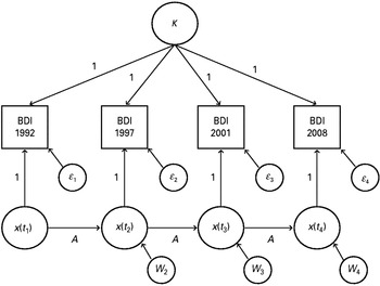
The model that we applied in the current study corresponds to a continuous version of the autoregressive latent trait–state model (Kenny & Zautra, Reference Kenny and Zautra1995; Cole & Martin, Reference Cole and Martin2005), shown in path analysis form in Fig. 1 (Bollen, Reference Bollen1989). The difference is that a time-continuous process x(t) is modeled instead of the four discrete successive latent variables that correspond to theoretically arbitrary measurement times t 1, t 2, t 3 and t 4 (here, the years 1992, 1997, 2001 and 2008). The applied model is more widely known as the linear stochastic differential equation model (Øksendal, Reference Øksendal2003; Oud & Delsing, Reference Oud, Delsing, Montfort, Oud and Satorra2010), but it is estimated here using a structural equation model with appropriate nonlinear constraints (Oud & Delsing, Reference Oud, Delsing, Montfort, Oud and Satorra2010). This model has also been referred to as the exact discrete model (EDM) because it is in exact equivalence with the underlying continuous time process (Oud & Delsing, Reference Oud, Delsing, Montfort, Oud and Satorra2010).
Path analysis model yielding the discrete time equivalent for the exact discrete model (EDM). See text for meaning of symbols.

For technical reasons, continuity is rarely modeled in practice, although it has long been recognized that the discrete approximation is problematic (Bartlett, Reference Bartlett1946). For example, when fitting a non-random autoregressive model specified simply by x(t i)=A dx(t i–1), then
 $${{x\lpar t_{i} \rpar \minus x\lpar t_{i \minus \setnum{1}} \rpar } \over {t_{i} \minus t_{i \minus \setnum{1}} }} \equals {{A_{d} \minus 1} \over {t_{i} \minus t_{i \minus \setnum{1}} }}x\lpar t_{i \minus \setnum{1}} \rpar\hfill $$
approximates to the continuous differential equation dx/dt= Ax but depends nonlinearly on the measurement time interval. Discrete approximation for the true A is (A d−1)/(t i−t i−1), not A d. Therefore, the opposite finding may seem apparent, even though the true underlying autoregression function in continuous time was larger in one study with longer measurement intervals than in another study with shorter intervals. The problems of discrete models for underlying continuous latent processes are discussed elsewhere in more detail (Oud & Delsing, Reference Oud, Delsing, Montfort, Oud and Satorra2010). Instead, the linear stochastic differential equation model is described in the following text.
Let us denote the depression score at time t as x(t). Using existing notation (Oud & Delsing, Reference Oud, Delsing, Montfort, Oud and Satorra2010), the description of the time evolution that is fitted to the data is of the form:
 $${{{\rm d}x\lpar t\rpar } \over {{\rm d}t}} \equals Ax\lpar t\rpar \plus b \plus k \plus G{{{\rm d}W\lpar t\rpar } \over {{\rm d}t}}.\hfill$$
According to the model, the instantaneous time evolution of depressive symptoms depends linearly (with the scalar coefficient A) on (i) the level of depressive symptoms, (ii) the population mean level through the scalar b, (iii) the individual long-term mean level (trait) through the population random variable κ, and (iv) the standard (Wiener/Brownian) random process dW(t)/dt, scaled with the scalar G. Although involving randomness, the process W is continuous in time, describing the cumulative sources of variation. In addition, each observation of the process x, or measurement of a single individual's depression score at time t i of measurement i, is modeled as:
 $$y\lpar t_{i} \rpar \equals x\lpar t_{i} \rpar \plus \epsiv _{i} \comma\hfill $$
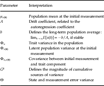
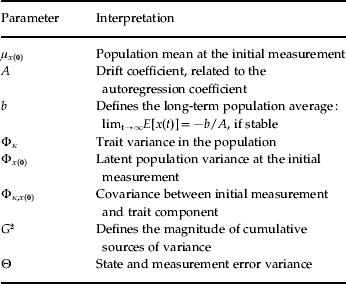
where εi is a normally distributed error term. Cov(εi)=Θ for all i, reflecting both measurement error and state fluctuations that are independent of the linear time evolution of equation (2). Hence, εi is independent of εj whenever i≠j. Table 1 summarizes the parameters of the process and their interpretations. The parameters are assumed to be the same for the whole sample of individuals included in the model estimation.
Interpretation of the model parameters
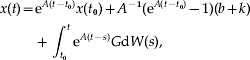
The solution of the stochastic differential equation (2) is
 $$\eqalign{x\lpar t\rpar \equals\tab {\rm e}^{A\lpar t \minus t_{\setnum{0}} \rpar } x\lpar t_{\setnum{0}} \rpar \plus A^{ \minus \setnum{1}} \lpar {\rm e}^{A\lpar t \minus t_{\setnum{0}} \rpar } \minus 1\rpar \lpar b \plus k\rpar \cr\tab\plus \int_{t_{\setnum{0}} }^{t} {{\rm e}^{A\lpar t \minus s\rpar } G{\rm d}W\lpar s\rpar } \comma}\hfill $$
where t 0 is the time of initial measurement; time can be rescaled so that t 0 is zero without a loss in generality (Øksendal, Reference Øksendal2003; Oud & Delsing, Reference Oud, Delsing, Montfort, Oud and Satorra2010). The last term on the right side of equation (4) is an instance of an Itô integral (Øksendal, Reference Øksendal2003; Klenke, Reference Klenke2008). From equation (4) and the rules of Itô integration, a formula can be derived for the variance of x(t). The variance is the sum of three terms that relate to initial depression value:
 $${\rm e}^{\setnum{2}A\lpar t \minus t_{\setnum{0}} \rpar } \rmPhi _{x\lpar \setnum{0}\rpar } \plus \tab 2{\rm e}^{A\lpar t \minus t_{\setnum{0}} \rpar } A^{ \minus \setnum{1}} \lpar {\rm e}^{A\lpar t \minus t_{\setnum{0}} \rpar } \minus 1\rpar \rmPhi _{k\comma x\lpar \setnum{0}\rpar } \comma\hfill$$
trait variation:
 $$A^{ \minus \setnum{2}} \lpar {\rm e}^{A\lpar t \minus t_{\setnum{0}} \rpar } \minus 1\rpar ^{\setnum{2}} \rmPhi _{k} \comma\hfill$$
and variance due to cumulative effect:
 $$\lpar 2A\rpar ^{ \minus \setnum{1}} \lpar {\rm e}^{\setnum{2}A\lpar t \minus t_{\setnum{0}} \rpar } \minus 1\rpar G^{\setnum{2}}. \cr}\hfill $$
In a stable process that does not increase or decrease without bounds, A is negative, implying that all variance components are positive at all times. The initial value of the contribution to variance [i.e. formula (5)] vanishes as time passes (i.e. the terms that depend on x(0): shorthand for x(t 0) in subindices). In the infinite time limit, the stable trait variance is A −2Φ κ, and variance due to cumulative effects is (2A)−1G 2. Variance due to the state/measurement error, Θ, relates to differences between the latent process of equation (4) and its measurement; Θ never depends on time. In the results section, the three-component variance decomposition of the measured depression score is presented for the infinite time limit. This is one way to interpret the course of depression without confounding due to variation in initial measurements, but we also present the decomposition at t−t 0=82.4; that is, after the modeled cumulative effects have accumulated for approximately the length of life expectation in high-income countries, as projected for the year 2030 (Mathers & Loncar, Reference Mathers and Loncar2006). The proportion of variance attributed to cumulative effects is plotted as a function of time in Fig. 3. In these time-specific calculations, the variance terms that depend on x(0) are simply excluded.
The EDM was estimated using OpenMx structural equation modeling software (Boker et al. Reference Boker, Neale, Maes, Wilde, Spiegel, Brick, Spies, Estabrook, Kenny, Bates, Mehta and Fox2011). The structural model and its nonlinear constraints were formulated as instructed in the literature (Oud & Delsing, Reference Oud, Delsing, Montfort, Oud and Satorra2010). The model was estimated with the full information maximum likelihood (FIML) approach that has been found successful in the modeling of missing data (Muthén et al. Reference Muthén, Kaplan and Hollis1987), even in the case of non-normal data (Enders, Reference Enders2001). Structural equation models were evaluated using the likelihood ratio test and Akaike's (AIC) and Bayesian (BIC) information criteria (Bollen, Reference Bollen1989; Kass & Raftery, Reference Kass and Raftery1995). A model that attains a lower value than the competing models is preferred according to AIC and BIC. Differences between sample skewness and that of normal distribution are assessed with the D'Agostino test for skewness, and differences in kurtosis with the Anscombe–Glynn test, as implemented in the Moments package, version 0.12, by Lukasz Komsta (http://cran.r-project.org/web/packages/moments/moments.pdf). Bootstrapping with 1000 bootstrap resamples of original data was used to derive percentile confidence intervals (CIs) for the EDM parameters (Efron & Tibshirani, Reference Efron and Tibshirani1993).
Latent trait modeling
Latent trait measurement modeling is often applied to increase measurement precision. We chose to model the time trajectories of the sum score, however, for the following three reasons. First, recent evidence supports the view that depression represents a causal network of symptoms rather than the view that the symptoms reflect a common latent cause (Cramer et al. Reference Cramer, Borsboom, Aggen and Kendler2012). Enforcing of the latent trait model with time-invariant loadings to data from a causal network would inflate the error/state component of the model: if one symptom for an individual is truly elevated between two measurement times but another symptom is not, then the model would tend to interpret the change as a random fluctuation (as the underlying latent variable change is expected to reflect all symptoms according to their loadings). Hence, modeling of the sum score was deemed as being consistent with clinical practice and with existing theoretical models, whether based on the latent trait or causal network. Second, efficient missing data handling would be difficult, as estimation should be based on the polychoric correlation matrix among the Likert-scaled items. Third, in a latent trait formulation, the state/error variance is a high-dimensional construct (dimension per item or symptom), complicating comparison with trait and cumulative variance parts of the model. In addition, the additional burden of estimation due to introducing several latent trait loadings and unique-variance terms might outweigh the gains in precision achieved from measurement modeling.
The two first arguments against latent trait modeling constitute a partially testable hypothesis whereas various solutions exist for the third. Therefore, we conducted the following supporting latent trait analysis. An empirical polychoric correlation matrix (Ekström, Reference Ekström2009) was computed for depressive symptoms over all follow-ups, and a latent-trait formulation of the EDM was estimated using the matrix; that is, loadings of the unidimensional latent process x(t) onto each depressive symptom, and the unique variances of the symptoms, were estimated along with the other model parameters (Oud & Delsing, Reference Oud, Delsing, Montfort, Oud and Satorra2010). The amount of observations required by OpenMx was set to a minimum over all two-variable margins among all 84 observed variables (21 symptoms×4 follow-ups). The median of unique variances represented the state/error variance. Infinite-time limits of trait, cumulative and state variances and their variability over the bootstrap samples were examined.
Results
Although depression measurements for the four time points (years 1992, 1997, 2001 and 2008) were not normally distributed, deviations from normal distribution kurtosis were barely detectable (p=0.089, 0.330, 0.038 and 0.040 respectively). Sample kurtosis varied between 2.893 and 3.241. Sample skewness varied between −0.6221 and −0.6169, with all p values <2.2×10⁻¹⁶. The magnitudes of these deviations from normality, however, are far below the values typically examined when bias due to non-normality is assessed for the FIML estimates in a structural equation context (Enders, Reference Enders2001). Hence, it seems safe to proceed without non-normality corrections that would add complexity for the present modeling aims.
In previous research, more stability in depression has been shown in adolescents than in children whereas greater cumulative effects have been found in children (Cole & Martin, Reference Cole and Martin2005). Thus, we first tested whether or not all six cohorts could be treated together. A likelihood ratio test was performed for a model with equal means and covariances for all cohorts versus the ‘saturated/unrestricted model’ with means and covariances varying freely across cohorts. This constitutes a test for the equality of mean and covariance structures between cohorts, with appropriate handling of the missing data achieved using the full information estimation. The difference between cohorts was almost significant (χ2=89.395, dfdifference=70, p=0.059), but BIC and AIC supported treating them as one set of data rather than as separate cohorts (−19051.17 v.−18 567.43 and 32 850.23 v. 32 900.84). Minor differences among cohorts might inflate the trait component of the EDM. We therefore performed the same test after removing the mean levels of all depression measurements for each cohort because the EDM is not needed to assess such a simple difference. This retains the time variation but removes overall mean differences among cohorts. After this adjustment it is safer to conclude that all cohorts can be analyzed together (χ2=85.863, dfdifference=70, p=0.096). Again, BIC (−19 010.18 v.−18 522.92) and AIC (32 891.22 v. 32 945.35) supported this choice.
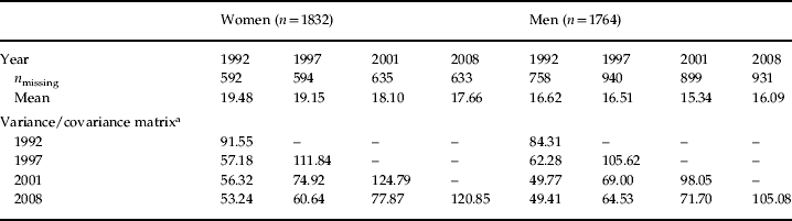
After the removal of the cohort means, we assessed whether it was possible to fit a single model combining men and women. The data suggested that solutions would be different for men and women, regardless of excluding the overall mean levels of sexes (p<1.362×10⁻¹¹ with or without). Thus, all further results are given separately for men and women. This solution was also favored by AIC (43 299.11 v. 43 352.82) and previous literature on depression (Nolen-Hoeksema & Girgus, Reference Nolen-Hoeksema and Girgus1994; Hankin et al. Reference Hankin, Abramson, Moffitt, Silva, McGee and Angell1998; Hyde et al. Reference Hyde, Mezulis and Abramson2008), but not by BIC (−8515.67 v. −8548.58), which penalizes more heavily from excess parameters (Kass & Raftery, Reference Kass and Raftery1995). Table 2 gives the FIML estimates of the saturated models. In practice, these correspond to sample means and covariance with less bias due to missing values than for the usual estimates of these quantities.
Estimated sample means and covariance for men and women
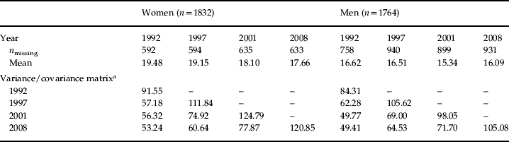
a Values on the diagonal are variances, other values are covariances among measurements. Only 177 women and 358 men lacked data each year.
Because cohort-wise differences in the time average of depression inflate the stable trait variance in the final EDM estimates, we removed these small differences before fitting the EDM for men and women. OpenMx's full information estimation algorithm did not converge successfully for the saturated (i.e. unrestricted/null) model when using the dummy variable required for the EDM's structural equation formulation (Oud & Delsing, Reference Oud, Delsing, Montfort, Oud and Satorra2010). This precluded proper nesting of EDM within the fully unrestricted missing-data model, which is necessary for the likelihood ratio test of model fit (Bollen, Reference Bollen1989). However, according to BIC and AIC, EDM supersedes the unrestricted model that was estimated without the EDM dummy variable for women (EDMBIC=−11 754.06 v. unrestrictedBIC=−1323.357; EDMAIC=25 173.11 v. unrestrictedAIC=25 470.62). The situation was similar for men (EDMBIC=−11 379.91 v. unrestrictedBIC=−1421.58; EDMAIC=17 551.79 v. unrestrictedAIC=17 818.76). Thus, from the model parsimony point of view, EDM seems to fit to the data in the absolute sense; evidence against the null model was very strong (Kass & Raftery, Reference Kass and Raftery1995). We then turned to individual parameter estimates.
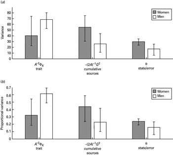
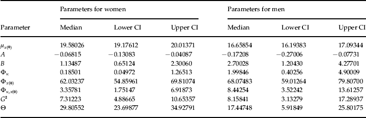
Table 3 gives the parameter estimates separately for men and women. Bootstrap distributions of parameters were fairly skewed, with heavy tails (probably due to nonlinear constraints that are needed in estimation of the EDM, and may even cause occasional failures in estimation). Hence, we present 90% CIs rather than the usual 95%. For the same reason, the less accurate but more robust percentile interval was used instead of the ‘bias corrected and accelerated’ interval, where the ‘acceleration’ estimates involve cubes of all deviations (Efron & Tibshirani, Reference Efron and Tibshirani1993). The parameter estimates allow calculation of the variance decomposition for the measured stochastic process, y [see equations (3), (6) and (7)]. Fig. 2 illustrates the estimated relative proportions of variance for stable trait, cumulative sources and state/error; it shows the proportional long run (infinite time) asymptotes of the respective components. Limiting values are more informative about the underlying population values because the data contain no information about how participants have arrived at the depression value observed at the initial measurement. For women, 32.2% of the variance (90% CI 18.5–54.2) was explained by the stable trait-like component, 43.9% (90% CI 23.6–58.9) by sources that accumulate in time and 23.9% (90% CI 19.1–27.3) by state fluctuation or measurement error. For men, 61.4% (90% CI 48.9–69.2) of variance was due to the stable trait, 23.0% (90% CI 9.9–41.7) to cumulative sources and 15.6% (90% CI 5.6–23.2) to state fluctuations. Precise decomposition between trait and cumulative sources was more difficult to obtain than the state variance, as shown by the CIs.
(a) Model-derived time limits of the three sources of variance: trait, cumulative effects and state/measurement error. The infinite time limit is taken because otherwise these quantities depend on the initial measurement, and we wanted to compare them generally. Error bars show 90% bootstrap percentile confidence intervals (CIs). (b) Relative proportions of variance among the three model components, with 90% CIs derived from bootstrap replications of the corresponding proportions.

Estimated parameters for the linear stochastic differential equation model

The lower confidence interval (CI) is the 5th bootstrap percentile from 1000 resamples and the upper CI is the 95th percentile. As in Table 1, the symbols refer to the population mean at the initial measurement (μx(0)), the drift coefficient (A), long-term population average (b), trait variance in the population (Φκ), latent population variance at the initial measurement (Φx(0)), covariance between the initial measurement and the trait component (Φκ,x(0)), defining parameter for the cumulative sources of variance (G 2), and the state and measurement error variance (Θ). The numbers are reported with a high precision to facilitate possible (nonlinear) calculations in future studies.
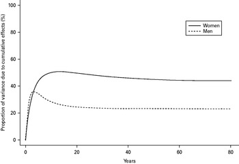
It is reasonable to ask whether the infinite time approximation corresponds well to variance shares observed in realistic time intervals. Therefore, we report proportional values for variance due to trait, cumulative effects and state, when an amount of time equal to life expectation in high-income countries has passed [i.e. variance decomposition for x(82.4+t 0)]. Variance terms dependent on the initial measurement point were excluded from the comparison. For women, 31.8% (90% CI 17.7–54.2) of the remaining variance share was attributed to the stable trait, 43.9% (90% CI 23.6–59.6) to the cumulative effects and 23.5% (90% CI 19.1–27.6) to the state effects. For men, 62.3% (90% CI 48.8–69.2) of the variance was attributed to the stable trait, 23.2% (90% CI 10.0–41.7) to the cumulative effects and 15.8% (90% CI 5.5–23.2) to the state effects. These values correspond very closely to observations in the infinite time limit. Fig. 3 shows how the proportion of variance attributed to cumulative effects first grows as time passes, and then settles near to an asymptote in about 20–40 years.
Proportion of variance due to cumulative effects (%) as opposed to trait and state effects, plotted as a function of time (years).

Finally, we tested the latent common cause formulation of the model, estimated from polychoric correlations. Because of frequent algorithmic failures and a high proportion of large deviations, bootstrap estimates would have varied considerably more than for the sum score, precluding reasonable CI estimates. Medians of 1000 bootstrap resamples for men and women were computed for a qualitative comparison between the latent trait model and the full information modeling of the sum score. The relative variance shares among the trait (17.1% for women, 20.7% for men), cumulative (43.5% for women, 37.5% for men) and state components (39.4% for women, 41.8% for men) replicated the gender tendencies for the sum score with the exception that the state/error component was considerably inflated; recall that the inflation of the error component was expected if the common cause assumption was wrong.
Discussion
This study examined the longitudinal course of depressive symptoms in adulthood, using the Young Finns follow-up data (Raitakari et al. Reference Raitakari, Juonala, Rönnemaa, Keltikangas-Järvinen, Räsänen, Pietikäinen, Hutri-Kähönen, Taittonen, Jokinen, Marniemi, Jula, Telama, Kähönen, Lehtimäki, Åkerblom and Viikari2008). Initially, 15- to 30-year-old participants were followed for 16 years. Four successive measurements were made, with 5-, 4- and 7-year intervals between them. The observed population variance of the course of depressive symptoms was decomposed into the three main sources: (1) individual differences in stable trait-like depression that may be caused by genetic differences, or by early experiences that determined time-constant levels of depressive symptoms for individuals; (2) individual differences that derive from a continuously accumulating trajectory of small changes, such as negative (or protective) cycles of deteriorating (or improving) mental health that influence the course of depression; and (3) differences due to state fluctuation or measurement error without continuity over time. In men, the stable trait accounted for the majority (61%) of the total variance, followed by cumulative effects (23%) and state fluctuations (16%) (Fig. 2). In women, the cumulative sources were more important than among men and accounted for 44% of the variance, followed by stable individual differences (32%) and state fluctuations (24%). In addition to the differences in the longitudinal course, women had a higher mean level and higher variance of depressive symptoms than men, in all follow-ups (Table 2).
The present data are in agreement with the previous observations that women have higher mean levels and higher variance of depressive symptoms than men (Nolen-Hoeksema & Girgus, Reference Nolen-Hoeksema and Girgus1994; Hankin et al. Reference Hankin, Abramson, Moffitt, Silva, McGee and Angell1998; Hyde et al. Reference Hyde, Mezulis and Abramson2008). The gender difference emerges by ages 13–15 years, that is before the first follow-up in the present data. One model explains the gender difference with women's greater biological (e.g. pubertal hormones), affective (temperamental) and cognitive (e.g. objectified body consciousness) vulnerabilities, which combine with a larger amount of environmental triggers (e.g. role pressures) than for men (Hyde et al. Reference Hyde, Mezulis and Abramson2008). The model emphasizes the role of interactions between many vulnerability factors and stressors in the emerging gender differences. Naturally, women may also continue to have more vulnerability–stressor interactions than men after puberty. Herein, the observed gender differences in the relative contributions of the estimated variance components suggest that men's level of depressive symptoms at a given time point is more a result of stable individual differences; whereas in women, time-dependent accumulating effects are more significant. Therefore, depressive symptoms of women are expected to change more than those of men in adulthood.
Previous studies have rarely decomposed the non-stable variance in depression into a state/error component versus a component that develops continuously over time. Here, it was estimated that <27% of variance is due to state-like fluctuations or measurement error. The rest is accounted for by autoregressive trajectories of depressive symptoms that accumulate over time differently for different participants, or by trait-like depression that stays constant for an individual, with between-individual variation in that constant. The latter share of the between-individual variance is either constitutional or has stabilized before adulthood. The cumulative part must be due to changes in the individual or in the environment that have occurred during the follow-up period of 16 years. Genetic effects can potentially enter the cumulative part only through gene–environment interactions (Brown & Harris, Reference Brown and Harris2008; Caspi et al. Reference Caspi, Hariri, Holmes, Uher and Moffitt2010), preprogrammed lagged effects or epigenetic effects (Zhang & Meaney, Reference Zhang and Meaney2010), but not as solid constitutional genetic effects. The cumulative proportion of intra-individual variation is not a measurement error, yet keeps changing in time.
In the current research literature on depression, the cumulative source of variation is the least well known among the three components accounting for the longitudinal course of depressive symptoms. Recall that we modeled an individual's time accumulating depression level using integration with respect to Brownian motion (also called the Wiener process). Brownian motion is a random process that is most frequently used to model a time trajectory of an agent or object that is continuously perturbed by many small outside influences (Øksendal, Reference Øksendal2003). For example, it is a model for a very small particle immersed in fluid and undergoing movement due to countless tiny collisions with the surrounding moving atoms. Instead of moving atoms, we model effects due to many small external and internal occurrences affecting depression and adding up in time. The fact that women were estimated to have more such occurrences is in line with the multiple pathways model that aims to explain the gender differences in depression (Hyde et al. Reference Hyde, Mezulis and Abramson2008). The time accumulation in a depression score might also reflect ‘kindling’ or a stress sensitization mechanism (Monroe & Harkness, Reference Monroe and Harkness2005). A Brownian motion-based model is compatible with the concepts of multi- and equifinality (Cicchetti & Rogosh, Reference Cicchetti and Rogosh1996) because same starting value of depression can develop to different outcomes at a later time; and different initial values can converge. In effect, unobserved influences may or may not cancel each other out as time passes.
The model of time accumulation that was applied here is closely related to an autoregressive time-series approach that was used in a prior study of children and adolescent depression, along with the trait and state components (Cole & Martin, Reference Cole and Martin2005). However, the present continuous-time model can be more readily compared with studies with different depression assessment-time intervals than the discrete-time autoregressive models (Oud & Jansen, Reference Oud and Jansen2000; Oud & Delsing, Reference Oud, Delsing, Montfort, Oud and Satorra2010). Using the parameter estimates in Table 3, various calculations become possible for depression trajectories, including the expected number of level crossings, and the mean and variance trajectories (Øksendal, Reference Øksendal2003; Klenke, Reference Klenke2008).
The findings of the present investigation also touch upon the issue of the theoretical underpinnings of depression. Attempts at modeling in terms of a time-evolving unidimensional latent common cause for depressive symptoms led to high variability of estimates. Nonetheless, and despite the very different technical implementation compared to sum score modeling, the most robust achievable (bootstrap median) estimates replicated the basic finding that the cumulative component plays a greater role for women than for men. In addition, the state/error part of the model was inflated relative to sum score modeling. Difficulties in estimation, and especially the inflation of error terms, are expected consequences if the underlying assumption of unidimensional common cause for symptoms is wrong (see Method). Therefore, although the evaluation of the common cause assumption was not the primary research question here, these observed phenomena are in line with recent evidence indicating that depressive symptoms reflect a causal network rather than unidimensional common cause (Cramer et al. Reference Cramer, Borsboom, Aggen and Kendler2012). Although problems due to the erroneous unidimensionality assumption are likely to be more prominent in longitudinal modeling, a sensitive cross-sectional measurement-theoretical analysis using a good data set revealed as many as six dimensions in a set of depressive symptom items (Uher et al. Reference Uher, Farmer, Maier, Rietschel, Hauser, Marusic, Mors, Elkin, Williamson, Schmael, Henigsberg, Perez, Mendlewicz, Janzing, Zobel, Skibinska, Kozel, Stamp, Bajs, Placentino, Barreto, McGuffin and Aitchison2008). If the sum score derives from symptoms forming a causal network, it is pushed and pulled by several separate contributions; in that case, Brownian movement seems an especially fitting model.
Limitations
More measurement points would facilitate better precision for the parameter estimates than that obtained here. Less uncertainty in parameters would directly translate to less uncertainty in the model-derived variance decomposition. Unfortunately, the present estimates had a high variance. The bootstrap estimates can be considered conservative, however, in the sense that they incorporate both the sampling variability and the variability due to algorithmic convergence issues; OpenMx cannot compute the usual sampling theory estimates when nonlinear constraints required by the stochastic differential equation model are used in estimation.
In addition to variability issues, information was not available regarding who (if any) of the participants had received treatment for depression. The participants were drawn from the general population of Finland. In that general population, the prevalence of antidepressant use was estimated to be 5.3% in the year 2000 (Sihvo et al. Reference Sihvo, Isometsä, Kiviruusu, Hämäläinen, Suvisaari, Perälä, Pirkola, Saarni and Lönnqvist2008), and rose steadily to 8.9% between 2000 and 2008 (Pulkki-Råback et al. Reference Pulkki-Råback, Kivimäki, Ahola, Joutsenniemi, Elovainio, Rossi, Puttonen, Koskinen, Isometsä, Lönnqvist and Virtanen2012). Nevertheless, not all users of antidepressants are depressed (Sihvo et al. Reference Sihvo, Isometsä, Kiviruusu, Hämäläinen, Suvisaari, Perälä, Pirkola, Saarni and Lönnqvist2008), and antidepressants seem to have a clear effect only for the severe cases of depression (Kirsch et al. Reference Kirsch, Deacon, Huedo-Medina, Scoboria, Moore and Johnson2008). Severe cases were scarcely present in our data as only 1.2% had a BDI-II score in the severe category (⩾29) in 2008. Therefore, treatment effects may impact the observed time trajectories only slightly.
Conclusions
A large proportion of the individual differences seen in male depressive symptoms are stable through the 16 years of adulthood studied here. They are less stable for women, who show more depression and larger variations in depression than men. For both genders, there is a distinctive part of the between-individual variance that exists due to different time trajectories. When only the presence of depression is modeled, the share of the state fluctuations and measurement error in the total depression variance is often estimated as being large (up to 67%): by contrast, it is unlikely to exceed 27% of the total variance when the longitudinal course of depressive symptoms is taken into account.
Acknowledgments
The Young Finns Study has received financial support from the Academy of Finland, the Social Insurance Institution of Finland, Kuopio, Tampere and Turku University Hospital Medical Funds, the Juho Vainio Foundation, Paavo Nurmi Foundation, Finnish Foundation of Cardiovascular Research and Finnish Cultural Foundation, Sigrid Juselius Foundation, Tampere Tuberculosis Foundation, and Emil Aaltonen Foundation. Expert technical assistance in data management by I. Lisinen and V. Aalto is gratefully acknowledged. Financial support has also been received from the Emil Aaltonen Foundation (M.H.), Ella and Georg Ehrnrooth Foundation (M.H.), Signe and Ane Gyllenberg Foundation (M.H. and L.K.J.), Niilo Helander Foundation (M.H.), the Academy of Finland [project numbers 123621 (L.P.R.) and 258711 (L.K.J.)], Research Foundation of the University of Helsinki (T.R.), and Oskar Öflund Foundation (T.R.).
Declaration of Interest
None.