I. INTRODUCTION
For decades, many studies have been conducted on the strain measurement in nanostructured materials. Strain can appear either as a beneficial or a detrimental factor originating from a lattice mismatch between layers of different composition, deposited during the epitaxial growth. It can affect the physical, electronic, optical, sensory, and magnetic properties of crystals. Strain can increase the mobility of the charge carriers by the band gap reduction. Continuous reduction of the feature size in semiconductor devices also increases the necessity of determining strain at the nanoscale. The strain effect in semiconductor device performance is perfectly known from the electrical point of view; however, very little is established about the strain profile in semiconductors. Reference Chun, Sun, Aghoram and Thompson1,Reference Sun, Thompson and Nishida2,Reference Ungersboeck, Dhar, Karlowatz, Sverdlov, Kosina and Selberherr26 The knowledge of the three-dimensional (3D) strain state at the nanoscale is important in the future quantum computers development, i.e., the band alignment due to the misfit strain enables quantum confinement is Si/SiGe buried channel structures. Reference Deelman, Edge and Jackson3
There are several transmission electron microscopy (TEM) techniques developed to measure strain in crystals. They include high resolution TEM (HRTEM), Reference Hӱtch, Snoeck and Kilaas4,Reference Hӱtch and Potez5 nanobeam electron diffraction, Reference Saitoh, Nakahara and Tanaka6,Reference Favia, Gonzales, Simoen, Verheyen, Klenov and Bender7 convergent beam electron diffraction (CBED), Reference Armigliato, Balboni, Carnevale, Pavia, Piccolo, Frabboni, Benedetti and Cullis8–Reference Clément, Pantel, Kwakman and Rouvière12,Reference Rozeveld and Howe27 and dark field electron holography (DFEH). Reference Cooper, Barnes, Hartmann, Béché and Rouvière13,Reference Béché, Rouvière, Barnes and Cooper14 These techniques determine strain at the nanometer scale ∼(2–6) nm within the xy-plane of the specimen. They all have a high sensitivity of 1 × 10⁻³–2 × 10⁻⁴ (Ref. Reference Béché, Rouvière, Barnes and Cooper15) to the atomic displacement. HRTEM and NBD are limited to the strain measurement in two dimensions. Several attempts have been done to evaluate the third dimension, the z-dependent strain profile. Vincent et al. Reference Vincent, Walsh and Pozzi16 suggested a direct Fourier transform of the rocking curves around the Bragg condition to retrieve the phase information of the diffracted beam at the exit surface of the specimen. Javon et al. Reference Javon, Lubk, Cours, Reboh, Cherkashin, Houdellier, Gatel and Hӱtch17 applied a weighting function on the average value of strain measured by DFEH to fit the z-dependent strain profile simulated by the finite element method. The accuracy of these techniques is highly influenced by the dynamical diffraction effects. Therefore, higher order reflections, which suffer less from dynamical diffraction, are always preferred. Reference Vincent, Walsh and Pozzi16–Reference Lubk, Javon, Cherkashin, Reboh, Gatel and Hӱtch18 CBED’s higher order Laue zone (HOLZ) lines are the most sensitive diffraction patterns to the atomic displacement and are less sensitive to the dynamical diffraction due to their large extinction distance, ξ. HOLZ lines split in the presence of a nonuniform atomic displacement along the beam direction, i.e., a bend. For kinematical simulations of the intensity profiles across the split HOLZ lines, the Howie–Whelan equation has been used, Reference Saitoh, Yasuda, Hamabe and Tanaka11,Reference Vincent, Walsh and Pozzi16,Reference Alfonso, Alexandre, Leroux, Jurczak, Saikaly, Charai and Penisson19 where the width of the HOLZ line split is related to the maximum atomic displacement through the specimen normal to the beam direction. Reference Saitoh, Yasuda, Hamabe and Tanaka11,Reference Vincent, Preston and King20 The width of the split HOLZ line is linearly related to the atomic displacement; Reference Saitoh, Yasuda, Hamabe and Tanaka11,Reference Vincent, Preston and King20 however, the split width does not provide sufficient information to fit the experiments to the models of the candidate strain profiles along the z-axis. It has been discussed that the intensity profile across the split HOLZ line carries the strain distribution and its profile along the z-axis. Although, the fringes of the internal intensity are too low of spatial frequency to obtain meaningful information. Required to recover the strain information along the beam direction is to measure the diffracted electron beam phase across the split HOLZ line, which is lost by recording the diffraction intensity. Reference Vincent, Walsh and Pozzi16,Reference Alfonso, Alexandre, Leroux, Jurczak, Saikaly, Charai and Penisson19,Reference Vincent, Preston and King20 The phase distribution across the split HOLZ line has been recently recoverable by Herring et al. (2015) using the novel technique of self-interference of split HOLZ line (SIS-HOLZ). Reference Herring, Norouzpour, Saitoh, Tanaka and Tanji21 Previously in Ref. Reference Herring, Norouzpour, Saitoh, Tanaka and Tanji21, it was reported that the bell-shaped strain profile is the best fit for the displacement distribution through the thickness of a thin specimen. Here, we report further details of the SIS-HOLZ technique using a spherical and coma aberration-corrected microscope. In Sec. II, the experimental details of the SIS-HOLZ technique are reported. The SIS-HOLZ is conducted close to the highly strained interface of a Si/Si0.8Ge0.2 superlattice on a Si substrate. The obtained results in Sec. III are finally discussed by the theoretical interpretations in Sec. IV and V.
II. EXPERIMENTAL PROCEDURE
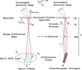
This technique is very similar to the diffracted beam interferometry method in terms of the experimental details. Reference Herring, Pozzi, Tanji and Tonomura22,Reference Herring, Pozzi, Tanji and Tonomura23 By applying a voltage on the biprism positioned in the middle of the split HOLZ line, two sides of the split are interfered giving the interference fringes (interferogram) on the diffraction plane. Fig. 1 shows a schematic of the SIS-HOLZ technique.
A simplified diagram of the SIS-HOLZ technique. By applying a voltage on the biprism, the intensities passing either of its sides deflect toward each other by an angle of αB to self-interfere. The specimen is Si/Si0.8Ge0.2 superlattices on the Si substrate. The ROI for conducting the experiment was in the Si substrate close to the interface that is strained due to the lattice mismatch between Si and Si0.8Ge0.2. Here, S1 is from the bottom half side of the specimen and S2 comes from the top half side of the specimen, if the beam is under-focused as in the diagram.

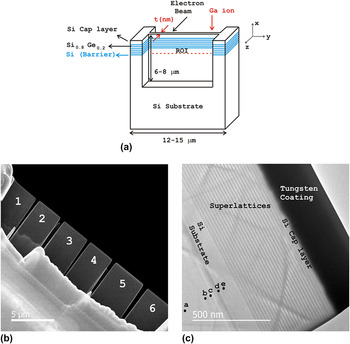
Regarding Fig. 2, the bulk sample in this work was a wafer of Si/Si0.8Ge0.2 superlattices on a Si substrate. The cross-section specimens were fabricated along the growth direction, [001] by the lift out technique using a focused ion beam, a Hitachi FIB-2100 (Hitachi Corp., Tokyo, Japan). Due to the sensitivity of the phase profile to the specimen condition, the specimen preparation was a challenging task. The following essential considerations were made for the specimen fabrication to avoid the strain state modifications and protect the cap layer.
-
(i) The top surface of the primary bulk specimen was coated by 15 nm of gold/palladium (Au/Pd) alloy using an Anatech Hummer VI (Au/Pd) sputtering system.
-
(ii) A few microns of tungsten were deposited on top of the Au/Pd coating to further avoid damaging the Si cap layer and the superlattices.
-
(iii) The final cut by the FIB should be done with a very low voltage beam to decrease the thickness of the FIB-induced damaged layer on the TEM specimen surface. 10 kV or 8 kV are often preferred. Reference Alexandre, Rousseau, Alfonso, Saikaly, Fares, Grosjean and Charai28 However, a 30 kV Ga+ ion beam was used in this work due to the instability of lower voltage beams. Every 10 kV energy adds ∼10 nm damaged layer on the surface. So ∼30 nm of damaged layer was expected on each surface of the specimen before further cleaning by ion milling.
-
(iv) As well, the specimen was attached by the FIB on top of a lift out copper grid, since during ion milling (101 Fischione) the copper will deposit onto the specimen’s surface modifying its strain state. The Ar+ beam of the ion miller was set to a glancing angle of ±15° with a 5 µA current and a 3 kV voltage. After milling each side for about 3–4 minutes, the specimen was cleaned to remove the surface radicals using a Hitachi UV Zone Cleaner for 10 min on each side.
(a) A schematic of the cross-sectioned specimen, made by the lift out technique using the FIB, (b) low magnification STEHM image of six fabricated specimens with different thickness variation, and (c) high magnification STEHM image of specimen 1 showing Si/Si0.8Ge0.2 superlattices, Si capping layer and tungsten coating.

The schematic of the fabricated specimen is given in Fig. 2(a). The Ga+ direction in the FIB and the electron-beam direction in the scanning transmission electron holography microscope (STEHM) are shown.
The measured specimen thickness using the electron energy loss spectroscopy (EELS) in the region of interest (ROI) is reported in Sec. III. The Hitachi HF-3300v STEHM having spherical and coma correction of its TEM mode operating at 200 kV was used to conduct the SIS-HOLZ experiment. This microscope is equipped with the following:
-
(i) A high coherence and high brightness field emission gun.
-
(ii) A rotatable electron biprism in the selected area aperture plane. The biprism is a thin wire of quartz covered with gold having a diameter of 0.35 µm with 2 mm length. It can move in both x and y directions (x: ±1 mm, y: ±1 mm) plus a 360 in-plane rotation enabling the biprism to be easily aligned parallel to any split HOLZ line.
-
(iii) A Gatan Ultrascan 2k × 2k CCD camera (Gatan Inc., Pleasanton, California) and an energy filtered GIF 2k × 2k camera using zero loss electrons. A 10 eV energy slit was used in this work to help with removing the background noise and the fringe contrast enhancement. The importance of the fringe contrast in the phase noise will be discussed further in Sec. V.
-
(iv) This experiment was conducted in the dark field (DF) disk of the CBED pattern to improve the contrast of the split HOLZ line. It also helps to recover only the strain information on the specific crystalline plane by removing any extra phase information from other diffracted beams as found in the bright field (BF) disk of the CBED pattern. As well, working in the DF disk, one can more easily find areas along the split HOLZ line that have not been phase shifted by other HOLZ lines intersections. The alignment of the biprism inside the split HOLZ line is made easier too.
The interferograms were produced in the diffraction mode; however, an initial alignment of the biprism was done in the imaging mode with the specimen slightly defocused by a few microns (6 μm for this experiment). This was done by adjusting the specimen height to see the diffracted beams in the image. The biprism defocus, Z OB − Z O, helps to focus the virtual sources, S1 and S2 on the Z 1 plane (Fig. 1). After aligning the biprism parallel to the split HOLZ line, the diffraction mode was chosen. Some small adjustment in the biprism alignment is usually needed to compensate for the electron rotation along the optical axis. The biprism was placed parallel and in the middle of the split HOLZ line, i.e., perpendicular to the HOLZ line’s g reflection. Before self-interfering the split HOLZ line, for the biprism alignment purposes, it was useful to apply a negative potential on the biprism to separate the intensity in the middle of the split.
In this work, the split HOLZ line was taken at about 80 nm distant within the silicon substrate from the interface of Si and Si/Si0.8Ge0.2. Depending on the separation of the sources, S1 and S2, which corresponds to the split width, the biprism voltage varies to make a fully overlapped interference pattern. The resulting interferogram was recorded by the GIF camera at a camera length of 30 m. The reconstruction of the phase image included a fast Fourier transform (FFT) of the interferogram, filtering a sideband and applying an inverse FFT on the sideband performed using Holoworks, a DigitalMicrograph subroutine of Gatan. A Gaussian window was used to filter the sideband in the frequency domain having a radius of 1/3 of the distance between the centers of the sideband and the central band.
III. EXPERIMENTAL RESULTS
In this work, six specimens were fabricated by FIB with different thickness variations. The STEHM images of the FIB fabricated specimens are presented in Fig. 2(b) showing the thinned specimens. The thickness variation of the thinned cross sections for specimens 1 and 2 were 165 ± 2 nm, for specimens 3 and 4 were 173 ± 5 nm, for specimen 5 was 208 ± 7 nm, and for specimen 6 was 172 ± 15 nm. The thickness was measured by EELS. The specimen which was chosen to conduct the experiment, specimen 1, had the least thickness variation. The STEHM image of specimen 1 with a higher magnification is given in Fig. 2(c), the Si cap layer can be seen that is protected by a ≈200 nm tungsten coating. The cumulative thickness of superlattices was about 500 nm. The labeled spots on Fig. 2(c) show the areas where the diffraction patterns in Figs. 3 and 4 are taken.
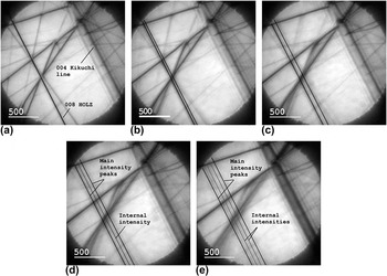
The 000 CBED disk obtained along the 004 Kikuchi band showing the HOLZ line taken within the Si substrate at (a) 400 ± 10 nm (no split), at (b) 200 ± 10 nm (begin to split), at (c) 180 ± 10 nm, (d) 100 ± 10 nm, and at (e) 70 ± 10 nm (the largest split) away from Si/Si0.8Ge0.2 interface.

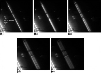
The DF disk 008 split HOLZ line obtained away from Si and Si0.8Ge0.2 interface at (a) 400 ± 10 nm, at (b) 200 ± 10 nm, at (c) 180 ± 10 nm, at (d) 100 ± 10 nm and, at (e) 70 ± 10 nm showing an increase in the split width approaching the interface.

In the strained region of the Si substrate, the HOLZ lines split into two intensity peaks with internal intensities within the split, Fig. 3. The internal low spatial frequency intensities appear at a certain distance from the interface, Fig. 3(d). Here, the internal fringes started to appear around 110–120 nm away from the Si/Si0.8Ge0.2 interface.
The 000 CBED HOLZ lines were taken in Si substrate of the specimen, along 004 Kikuchi band away from 100 zone axis. 008 HOLZ line could be seen clearly in the zoom mode, too. Therefore, the distances from the interface of Si substrate and Si/Si0.8Ge0.2 superlattices for the labeled spots in Fig. 2(c) are estimated roughly by observing the HOLZ line split width with respect to the interface in the image mode while moving the probe towards the interface. The split width has a linear relationship with the atomic displacement amplitude. Reference Saitoh, Yasuda, Hamabe and Tanaka11,Reference Vincent, Preston and King20 Thus, further away from Si/Si0.8Ge0.2 interface, the split width is decreased until at a large distance of ≥400 nm from the interface nonsplit, nonbroadened HOLZ line with no dynamical effects is observed, Fig. 3(a). Figure 4 shows the corresponding split HOLZ line in 004 and 008 DF disks compared to the 000 CBED disk in Fig. 3. The bright band on the bottom left side shows the 004 Kikuchi band. The DF disk split HOLZ lines have a higher contrast compared to their corresponding ones in BF disk making it easier to follow the trend in the splitting of HOLZ line while moving towards the interface. At about 80 nm away from the Si/Si0.8Ge0.2 interface [Fig. 4(e)] the split HOLZ line is wide and symmetric, which is a good condition to self-interfere. The split width and its symmetry importance will be discussed in Sec. V.
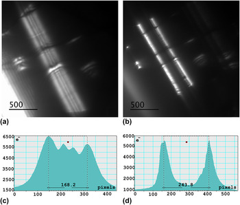
Figure 5, shows the intensity profiles across the split HOLZ line without [Fig. 5(c)] and with [Fig. 5(d)] a biprism inserted within the split having a negative potential to separate the intensity into two halves. There are two high intensity and two lower intensity fringes within this split HOLZ line, Figs. 5(a) and 5(c). The biprism placed in the center of the split HOLZ line, Fig. 5(b), cannot be seen except for its shadow running the length of the HOLZ line. On either of its sides there are two high intensity peaks, Fig. 5(d), having a reasonably symmetric intensity distribution. This is achieved by adjusting iteratively the virtual sources using the biprism defocus and the electron-beam cross over position. Figure 5(c) shows the split width of ≅168 pixels. A factor of 8.67 × 10⁻⁶ rad/pix was determined for the pixel conversion into the angular deflection, Δθ, which is 1.45 × 10⁻³ rad.
(a) The DF disk 008 split HOLZ line, (b) the biprism with a negative potential centered within the split HOLZ line for the alignment purposes, (c) the intensity distribution across the split HOLZ line in (a), and (d) the intensity profile while the biprism is centered inside the split HOLZ line.

These two peaks were finally interfered using a positive biprism potential. The applied voltage to fully overlap S1 and S2 taken at 80 nm away from the Si/Si0.8Ge0.2 interface was 4.5 V.
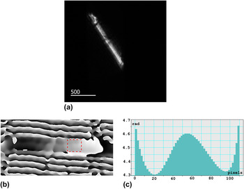
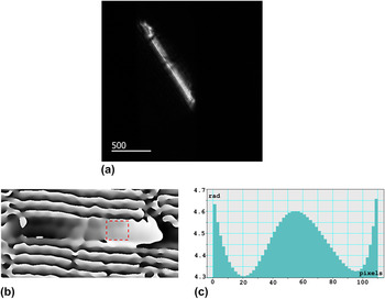
The self-interfered split HOLZ line interferogram was recorded with the GIF camera and an acquisition time of 5 s. The recorded interferogram, its reconstructed phase image and its phase profile are presented in Fig. 6. The phase profile is obtained across the boxed area in Fig. 6(b). It was preferred to avoid extra phase shift due to other HOLZ lines intersections. The phase profile in Fig. 6(c) shows a good agreement with a cosine bell-shaped displacement profile through the thickness of the crystal along the z-axis. The phase simulation details for a bell-shaped displacement profile are presented in Sec. IV.
(a) The interferogram of the self-interfered split HOLZ line showing fine fringes running parallel with the length of the HOLZ line, (b) the reconstructed phase image of (a) tilted horizontally for the presentation, (c) the phase profile passing through its width across the sketched box within the phase image.
IV. THE SIS-HOLZ ANALYTICAL DETAILS
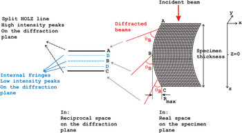
The path length of the electron beam changes passing through a bent crystal which is observed as a split of the intensity peaks, Fig. 7. HOLZ lines, which are high-angle, elastically Bragg diffracted electrons, split into two main intensities with some internal low frequency intensities (Figs. 3 and 4). The width of the split is linearly related to the displacement of the atomic planes. Reference Saitoh, Yasuda, Hamabe and Tanaka11,Reference Vincent, Preston and King20
 $$s = {{8\left| {{\bf{g}}.{\bf{R}}} \right|} \over t}\quad ,$$
where s defines the deviation from the exact Bragg angle of a perfect crystal, t is the specimen thickness, g is the HOLZ line diffraction vector, and R is the atomic displacement vector. Assuming g is parallel to R,
 $\left| {{\bf{g}}.{\bf{R}}} \right| = \left| g \right|\left| R \right|$
where R is the amplitude of the z-dependent displacement profile of R(z). Due to the strain relaxation at the specimen’s surfaces, R(z) is often assumed as a V-shape, a bell-shape, or a parabola profile through the thickness of the thin crystal holding no strain on the surfaces.
Reference Saitoh, Yasuda, Hamabe and Tanaka11,Reference Alfonso, Alexandre, Leroux, Jurczak, Saikaly, Charai and Penisson19,Reference Vincent, Preston and King20
The bell-shaped function was previously found to be the best fit for the displacement profile variation through the thickness of the specimen.
Reference Herring, Norouzpour, Saitoh, Tanaka and Tanji21
A schematic of a hypothetical z-dependent displacement profile of a bent crystal that Bragg diffracts the electron beam by the Bragg angle, θB. Due to the bent atomic planes, the constant θB keeps on tilting and deviating from its position for a perfect crystal causing the individual HOLZ line to split.

Considering a symmetrical bend about z = 0, at B in the middle of the foil in Fig. 7, in the reciprocal space, s is zero. ±s max happen at points A and C in the illustrated split. In addition to the split width and the internal intensities (A to D) which carry the strain information, the phase distribution across the split HOLZ line measures the electron-beam directional changes due to the bent atomic planes along the z-axis. By inserting a biprism in the center of the split, at B, and applying a small voltage on the biprism, the halves on the top and the bottom of B interfere and produce interfering fringes.
Regarding Fig. 7, the intensity of the diffracted beam lies in different locations from A to D due to the bending. Since there is a symmetric bend about the center of the crystal, A and C are the main split peaks with the same intensity. D lines also show equal intensities.
To calculate the phase profile, the diffracted beam equation at the exit surface of the specimen is split into two halves, performed experimentally using the biprism. Then the waves are deflected toward each other by a deflection angle, αB, for their interference. The resultant wave function carries the phase information across the split HOLZ line. To calculate the wave function, the principle wave equations in Ref. Reference Herring, Pozzi, Tanji and Tonomura22 are used. By following the beam propagation from the electron source to the specimen plane, to the biprism, and to the observation plane, the contribution of four terms in the phase factor of the diffracted waves are reported as follows:
-
(i) The biprism effect.
-
(ii) The complex factors representing the spherical aberration (the pre-specimen field, and the post-specimen field).
-
(iii) The defocus.
-
(iv) The microscope’s transmission function.
The spherical aberration and the defocus are both in γA and γB terms of Eq. (2) and Eq. (3) where “A” denotes the pre-specimen lenses and “B” represents the post-specimen lenses. The effect of a simple transmission function, T, in real space, exp(2πiK·r), whose Fourier transform is δ(k−K), is simply a rigid displacement of the wave vector on the diffraction plane, k, by K. All other phase factors are discussed comprehensively in Ref. Reference Herring, Pozzi, Tanji and Tonomura22. The final image wave function, Φ, is the sum of the two contributions coming from the left side (
 $\phi _{{\rm{shifted}}}^ -$
) and the right side (
 $\phi _{{\rm{shifted}}}^ +$
) of the biprism,
 $$\eqalignb{ & \phi _{{\rm{shifted}}}^ - = {\Sigma _{{\rm j}{{\rm{\bf S}}_{\bf 1}}}}{A_{{\rm \bf j}{{\rm{\bf S}}_{\bf 1}}}}\exp \left( { - 2\pi i{{\bf{g}}_{{\bf{j}}1}}.{\bf{R}}(z)} \right)\exp \left( { - 2\pi {\rm{i}}{{\rm\bf S_1}}.{\bf{r}}} \right) \cr & \quad \quad \times T\left( {{\bf{k}} + {{\bf{K}}_{\bf{B}}} - {{\bf{K}}_{\bf{T}}}} \right) \cr & \quad \quad \times \exp \left( { + 2\pi {\rm{i}}{{\bf{K}}_{\bf{B}}}.{{\bf{r}}_{\bf{B}}}} \right) \cr & \quad \quad \times \exp \left( { - {\rm{i}}{\gamma _{\rm{A}}}\left| {{\bf{k}} + {{\bf{g}}_{{\bf{j}}1}} + {{\rm \bf {S_1}}} + {{\bf{K}}_{\bf{B}}}} \right|} \right) \cr & \quad \quad \times \exp \left( { - {\rm{i}}{\gamma _{\rm{B}}}\left| {{\bf{k}} + {{\bf{K}}_{\bf{B}}}} \right|} \right)\quad , \cr}$$
 $$\eqalignb{ & \phi _{{\rm{shifted}}}^ + = {{\rm{\Sigma }}_{{\rm{j}}{{\bf{S}}_2}}}{{\rm{A}}_{{\rm{j}}{{\bf{S}}_2}}}\exp \left( { - 2{\rm{\pi i}}{{\bf{g}}_{{\bf{j}}2}}.{\bf{R}}({\rm{z}})} \right)\exp ( - 2{\rm{\pi i}}{{\bf{S}}_2}.{\bf{r}}) \cr & \quad \quad \times T\left( {{\bf{k}} - {{\bf{K}}_{\bf{B}}} - {{\bf{K}}_{\bf{T}}}} \right) \cr & \quad \quad \times \exp \left( { - 2{\rm{\pi i}}{{\bf{K}}_{\bf{B}}}.{{\bf{r}}_{\bf{B}}}} \right) \cr & \quad \quad \times {\rm{exp}}\left( { - {\rm{i}}{{\rm{\gamma }}_{\rm{A}}}\left| {{\bf{k}} + {{\bf{g}}_{{\bf{j}}2}} + {{\bf{S}}_2} - {{\bf{K}}_{\bf{B}}}} \right|} \right) \cr & \quad \quad \times {\rm{exp}}\left( { - {\rm{i}}{{\rm{\gamma }}_{\rm{B}}}\left| {{\bf{k}} - {{\bf{K}}_{\bf{B}}}} \right|} \right)\quad . \cr}$$
K
T
is a rigid displacement in the frequency space due to the interaction with any deflecting field other than the specimen and the biprism. K
T
is identical in both interfering beams and will be removed from the final wave function.
 ${{\rm{A}}_{{{\rm{S}}_1}}}$
and
 ${{\rm{A}}_{{{\rm{S}}_2}}}$
denote the amplitudes of the split HOLZ line from two left and right halves of the split. j is an integer showing the array of the replicas of diffracted intensities deviated from the exact Bragg position due to the bend, and i is the complex number.
 ${{\bf{g}}_{{\bf{j}}1}} = {{\bf{g}}_{{\bf{j}}2}}$
is the reciprocal wave vector of the HOLZ line and S
1 and S
2 are the two left and right halves of split (Fig. 1). r
B
is the coordinate of a generic point on the biprism axis and K
B
= (αB/λ)b is the rigid displacement of the beam due to the deflection angle, αB, b is the unit vector perpendicular to the biprism, and λ is the electron wave length. The extra phase factor of exp(±2πiK
B
.r
B
) is attributed to the biprism displacement effect. It is neglected in this work due to the biprism adjustment in the center of the spit, parallel with the HOLZ. The observation carried out in the diffraction mode and the general interferogram intensity is given by
 $$I = {\left| \Phi \right|^2} = {\left| {\phi _{{\rm{shifted}}}^ - + \phi _{{\rm{shifted}}}^ + } \right|^2}\quad .$$
Regarding Eq. (1), the half of the split width is s/2 = |S 1| = |S 2| = +4|g.R|/t. A perfect overlap occurs when the biprism is parallel and adjusted in the center of the split, |S 1| = |S 2|. This means K B = S 1 = −S 2. Therefore, the aberration term of γA in Eqs. (2) and (3) will be identical and they will drop out from the resultant wave function and the intensity equation. Reference Herring, Pozzi, Tanji and Tonomura22 In the phase calculation, the ideal imaging is considered and the spherical aberration is neglected. The spherical aberration will be displayed in the position dependency of the fringe spacing and the orientation of the interference pattern. Also, if the defocus value is large, the spherical aberration effect can be neglected. Reference Herring, Pozzi, Tanji and Tonomura22 However, these phase factors can be detected by the careful measurements of the fringe spacing as previously reported. Reference Gatel, Houdellier and Hӱtch24 In this work, spherical and coma aberration-corrected TEM was used so the post-field aberration, γB, is removed in the experiments which is also neglected in the calculations. This simplifies the mathematical analysis of the phase profiles and gives a closer fit between the experiment and simulation. Finally, all the additional complicated terms are pulled out in the diffracted beams [Eq. (2) and (3)] and the remaining term is the effect of the biprism due to the angle of deflection, exp(±2πiK B .r).
 $$\phi _{{\rm{shifted}}}^ - = {{\rm{\Sigma }}_{{\rm{j}}{{\bf{S}}_1}}}{A_{{\rm{j}}{{\bf{S}}_1}}}\exp \left( { - 2{\rm{\pi i}}{{\bf{g}}_{{\bf{j}}1}}.{\bf{R}}(z)} \right)\exp ( - 2{\rm{\pi i}}{{\bf{S}}_1}.{\bf{r}}) \times \exp \left( { - 2{\rm{\pi i}}{{\bf{K}}_{\bf{B}}}.{\bf{r}}} \right)$$
 $$\phi _{{\rm{shifted}}}^ + = {{\rm{\Sigma }}_{{\rm{j}}{{\bf{S}}_2}}}{A_{{\rm{j}}{{\bf{S}}_2}}}\exp \left( { - 2{\rm{\pi i}}{{\bf{g}}_{{\bf{j}}2}}.{\bf{R}}(z)} \right)\exp ( - 2{\rm{\pi i}}{{\bf{S}}_2}.{\bf{r}}) \times \exp \left( { + 2{\rm{\pi i}}{{\bf{K}}_{\bf{B}}}.{\bf{r}}} \right)\quad.$$
The first terms in Eq. (5) and (6) can be considered as the discrete forms of the Howie–Whelan equation for an imperfect crystal, Eq. (7). Reference Hirsch, Howie, Nicholson, Pashley and Whelan25
 $$\!\!\!\!\!{{\rm{\Phi }}_{\rm{g}}}(s) = {{{\rm{i\pi }}} \over {{{\rm{\xi }}_{\rm{g}}}}}\int_{ - {t \mathord{\left/ {\vphantom {t 2}} \right. \kern-\nulldelimiterspace} 2}}^{{t \mathord{\left/ {\vphantom {t 2}} \right. \kern-\nulldelimiterspace} 2}} \!\!{\exp \left( { - 2{\rm{\pi i}}sz} \right)\exp \left( { - 2{\rm{\pi i}}{\bf{g}}.{\bf{R}}\left( {\bf{z}} \right)} \right){\rm{d}}z} \quad ,$$
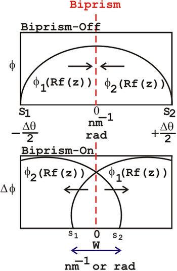
where Φg(s) is the diffracted wave and ξg is the extinction distance of the g reflection representing the HOLZ line. −2πig.R(z) that carries the z-dependent atomic displacement is in the phase term of the diffracted beam. Therefore, the Howie–Whelan equation solution predicts the total wave function at the exit surface of the specimen. As it is presented schematically in Fig. 8, the left and the right sides of the split are interfered to recover the phase profile (φ) across the split HOLZ line. In Fig. 8, the phase is shown in two parts of ϕ1(Rf(z)) and ϕ2(Rf(z)), which represent the left and the right sides of the phase across the split HOLZ line. S1 and S2 correspond to ±Δθ/2, where Δθ is the angular deflection from the exact Bragg angle. W shows the interference width. The SIS-HOLZ experimental phase profile is the outcome of the shown overlap.
A schematic of the phase profile across the split HOLZ line. When the biprism is off, there is no interference and only the split HOLZ line can be seen. When the biprism is on, the left and the right halves interfere.

It is assumed that the bend is symmetric about the center of the specimen at z = 0 in Fig. 7. Referring to Ref. Reference Saitoh, Yasuda, Hamabe and Tanaka11, R(z) can be simplified. The R(z) direction is considered consistent with respect to the g reflection and the z-dependent strain profile is indicated as Rf(z) where R is a scalar representing the strain amplitude, and f(z) shows the strain profile through the specimen thickness. The development of the analytical techniques presented in Ref. Reference Alfonso, Alexandre, Leroux, Jurczak, Saikaly, Charai and Penisson19 leads to the Howie–Whelan solution. In this work, a cosine bell-shaped function is considered for the displacement profile, f(z). The goal is to determine
 $${{\rm{\Phi }}_{{\rm{g}}{{\rm{S}}_1}}} = {{\rm{\Sigma }}_{{\rm{j}}{{\rm{S}}_1}}}{A_{{\rm{j}}{{\rm{S}}_1}}}\exp \left( { - 2{\rm{\pi i}}{{\rm{S}}_1}z} \right)\exp \left( { - 2{\rm{\pi i}}{\bf{g}}.{\bf{R}}\left( z \right)} \right)$$
and
 $${{\rm{\Phi }}_{{\rm{g}}{{\rm{S}}_2}}} = {{\rm{\Sigma }}_{{\rm{j}}{{\rm{S}}_2}}}{A_{{\rm{j}}{{\rm{S}}_2}}}\exp \left( { - 2{\rm{\pi i}}{{\rm{S}}_2}z} \right)\exp \left( { - 2{\rm{\pi i}}{\bf{g}}.{\bf{R}}\left( z \right)} \right)\quad ,$$
which correspond to the diffracted beams coming from the left and the right sides of the split HOLZ line. Assuming
 ${{\rm{\Phi }}_{{\rm{g}}{{\rm{S}}_1}}}$
and
 ${{\rm{\Phi }}_{{\rm{g}}{{\rm{S}}_2}}}$
are from the bottom half and the top half of the specimen, respectively, while the origin is z = 0. Regarding Fig. 1 showing an under-focused probe i.e., a focus below the specimen, S
1 and S
2 stem from the bottom half and top half of the specimen, respectively. Therefore,
 ${{\rm{\Phi }}_{\rm{g}}}\left( s \right) = {{\rm{\Phi }}_{{\rm{g}}{{\rm{S}}_1}}} + {{\rm{\Phi }}_{{\rm{g}}{{\rm{S}}_2}}}$
. To find, Φg(s), Eq. (7) is solved for two different boundaries as follows:
 $$\eqalignb{ & {{\rm{\Phi }}_{\rm{g}}}(s) = {{{\rm{i\pi }}} \over {{{\rm{\xi }}_{\rm{g}}}}}\int_{ - {t \over 2}}^0 {\exp \left( { - 2{\rm{\pi i}}sz} \right)\exp \left( { - 2{\rm{\pi i}}{\bf{g}}.{\bf{R}}\left( z \right)} \right){\rm{d}}z} \cr & {{{\rm{i\pi }}} \over {{{\rm{\xi }}_{\rm{g}}}}}\int_0^{{t \mathord{\left/ {\vphantom {t {\rm{2}}}} \right. \kern-\nulldelimiterspace} {\rm{2}}}} {\exp \left( { - 2{\rm{\pi i}}sz} \right)\exp \left( { - 2{\rm{\pi i}}{\bf{g}}.{\bf{R}}\left( z \right)} \right){\rm{d}}z} \quad . \cr}$$
To apply the SIS-HOLZ technique analytically, the bell-shaped displacement profile is substituted into
 ${{\rm{\Phi }}_{{\rm{g}}{{\rm{S}}_1}}}$
and
 ${{\rm{\Phi }}_{{\rm{g}}{{\rm{S}}_2}}}$
and the rigid shift of ±k
B
is added to each due to the biprism effect. For the simplification, let
 ${\rm{\Phi }}_{{\rm{shifted}}}^ - = {{\rm{\Phi }}_{{\rm{g}}{{\rm{S}}_1}}}{\rm{exp}}\left( { - 2{\rm{\pi i}}{{\bf{k}}_{\bf{B}}}.{\bf{r}}} \right)$
and
 ${\rm{\Phi }}_{{\rm{shifted}}}^ + = {{\rm{\Phi }}_{{\rm{g}}{{\rm{S}}_2}}}{\rm{exp}}\left( { + 2{\rm{\pi i}}{{\bf{k}}_{\bf{B}}}.{\bf{r}}} \right)$
. The resultant wave function is
 $${\rm{\Phi }}\left( s \right) = {\rm{\Phi }}_{{\rm{shifted}}}^ - + {\rm{\Phi }}_{{\rm{shifted}}}^ + \quad .$$
Here a cosine function is considered for the bell-shaped displacement profile as follows:
 $${\bf{R}}\left( z \right) = Rf\left( z \right) = {{R\left( {{\rm{cos}}\left( {{{2{\rm{\pi }}z} \over t}} \right) + 1} \right)} \mathord{\left/ {\vphantom {{R\left( {{\rm{cos}}\left( {{{2{\rm{\pi }}z} \over t}} \right) + 1} \right)} 2}} \right. \kern-\nulldelimiterspace} 2}\quad .$$
In this equation, zero displacement is at z = ±t/2 and the maximum displacement happens in the center. Due to the surface relaxation, it is expected to have the same z-dependent displacement profile in very thin specimens. However, depending on the specimen fabrication procedure, there are usually some strain modifications on the surfaces due to the damage. After the mathematical developments, finally the wave equation, Eq. (11), for the bell-shaped displacement profile, turns to
 $$\eqalignb{ & \Phi \left( s \right) = {{{\rm{i}}\pi } \over {{\xi _{\rm{g}}}}}\exp \left( { - M} \right)[{J_0}\left( M \right)\left( {\exp \left( { - \pi {\rm{i}}sN} \right) + \exp \left( {\pi isN} \right)} \right)\sin \left( {{{\pi st} \mathord{\left/ {\vphantom {{\pi st} 2}} \right. \kern-\nulldelimiterspace} 2}} \right)/\pi s \cr & + \sum\limits_{n = + 1}^{n = + \infty } {{{\left( i \right)}^n}{J_n}\left( M \right)\left( {\exp \left( { - \pi {\rm{i}}\left( {s + {n \over t}} \right)N} \right) + \exp \left( {\pi {\rm{i}}\left( {s + {n \over t}} \right)N} \right)} \right)\sin \left( {{{\pi \left( {s + n/t} \right)t} \mathord{\left/ {\vphantom {{\pi \left( {s + n/t} \right)t} 2}} \right. \kern-\nulldelimiterspace} 2}} \right)/\pi \left( {s + n/t} \right)} \cr & + \sum\limits_{n = + 1}^{n = + \infty } {{{\left( i \right)}^n}{J_n}\left( M \right)\left( {\exp \left( { - \pi {\rm{i}}\left( {s - {n \over t}} \right)N} \right) + \exp \left( {\pi {\rm{i}}\left( {s - {n \over t}} \right)N} \right)} \right)\sin \left( {{{\pi \left( {s + n/t} \right)t} \mathord{\left/ {\vphantom {{\pi \left( {s + n/t} \right)t} 2}} \right. \kern-\nulldelimiterspace} 2}} \right)/\pi \left( {s - n/t} \right)} \quad , \cr}$$
where M = 2πgR, N = t/2 − 2K B .r, and J n is the nth order Bessel function which appears by the integration of the Howie–Whelan equation for the bell-shaped atomic displacement. According to Eq. (7), the diffracted beam, Φg(s) is proportional to the Fourier Transform (FT) of the extra phase factor due to the strain, i.e., exp(−2ig.R(z)), convolved with a slit function of sin(πst)/(πs) written as a sinc(πs) function. Reference Alfonso, Alexandre, Leroux, Jurczak, Saikaly, Charai and Penisson19,Reference Vincent, Preston and King20 The Fourier transform of exp(−M cos(2πBz)) is Reference Alfonso, Alexandre, Leroux, Jurczak, Saikaly, Charai and Penisson19
 $$\sum\limits_{ - \infty }^{ + \infty } {{{\left( { - 1} \right)}^n}{{\left( { - {\rm{i}}} \right)}^n}{J_n}\left( {{\rm{i}}M} \right)\delta \left( {z - nB} \right)} \quad .$$
Thus, M = 2πgR and B = 1/t for a cosine function.
The analytical expression of the image wave function, Eq. (11), is applied to calculate the phase profile for the 008 split, using
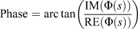 ${\rm{Phase}} = {\mathop{\rm arc}\nolimits} \,{\rm tan}\left( {{{{\rm{IM}}\left( {\Phi \left( s \right)} \right)} \over {{\rm{RE}}\left( {\Phi \left( s \right)} \right)}}} \right)$
, where IM(Φ(s)) and RE(Φ(s)) are the imaginary and real parts of Eq. (11), respectively.
The assumptions to calculate the phase profile with the explained approach are
-
(i) A perfect overlap is considered. The biprism is perfectly centered inside the split HOLZ line. So the extra phase factor of exp(±2πiK B .r B ) is neglected.
-
(ii) The biprism’s Fresnel fringe effect due to the diffraction from the edge of the biprism is neglected.
-
(iii) The pre-field and the post-field aberrations, γA and γB are removed by a perfect overlap and considering an aberration-corrected imaging.
-
(iv) In the defined bell-shaped displacement model, strain relaxation on the surfaces is considered.
-
(v) The diffraction vector g is considered parallel to the displacement vector, R.
Finally, the calculated phase profile is compared with the obtained experimental profile.
All the detailed experimental steps explained in Sec. II such as the specimen fabrication, the biprism defocus adjustment, the biprism alignment in the center of the split parallel to the HOLZ line and conducting the experiment using a spherical + coma aberration-corrected TEM confirm the validity of the mentioned phase calculation assumptions within a good approximation.
Also the experimental interference width, W, to the split HOLZ line ratio is 0.65s. This value is used as a window to pick the right spatial frequency boundaries in the phase calculations. Finally, the calculated phase profile is plotted versus Δθ using Δθ = s/g.
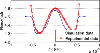
In Fig. 9, the cosine bell-shaped profile is in a good agreement with the experimental result. In practice the specimen is tilted 1.4° to bring the 008 deficiency HOLZ line into the 000 CBED disk; however, it is neglected in the phase calculation. Therefore, in Eq. (7),
 $\left| {\bf{g}} \right|\left| {\bf{R}} \right|$
substitutes the dot product of
 $\left| {{\bf{g}}.{\bf{R}}} \right|$
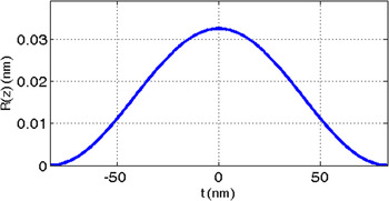
in the phase factor. The deviation between the calculated and the experimental profile is likely due to the small biprism misalignment, which is not considered in the simulation. By considering the bell-shaped displacement profile, Eq. (10), finally, the calculated R(z) along the z-axis is presented in Fig. 10. No strain is held by the surfaces of the thin specimen. The maximum atomic displacement amplitude ratio with respect to the Si lattice constant, a = 0.5431 nm, at about 80 nm away from the interface is 0.059 nm/nm. This large strain measured at the interface of the Si substrate and Si/Si0.8Ge0.2 superlattice may be due to the strain within the superlattice and not simply due to the added Ge where the strain within the Si and Si0.8Ge0.2 superlattice may not be fully relaxed.
The calculated phase profile is compared with the experimental phase profile showing a reasonably good fit.

The displacement profile at 80 nm distance from the interface along the z-axis, which is through the thickness of the crystal.

Here, the maximum atomic displacement R = 0.0325 nm happens at the center, z = 0. At t/2 ≅ ±83 nm from the top and bottom surfaces, the strain is zero. The inserted specimen thickness in the calculations was 166 nm, which fits in the specimen 1 thickness variation.
V. DISCUSSION
The phase across the split HOLZ line was not measureable until the SIS-HOLZ method produced high contrast, high spatial frequency interference fringes within the split HOLZ line.
The simplified SIS-HOLZ interferogram intensity is
 $$I = {\rm{\Phi }}\left( s \right){\rm{\Phi }}{\left( s \right)^{\rm{*}}} = {\left( {{a_{{\rm{g}}{{\rm{S}}_1}}}} \right)^2} + {\left( {{a_{{\rm{g}}{{\rm{S}}_2}}}} \right)^2} + 2{a_{{\rm{g}}{{\rm{S}}_1}}}{a_{{\rm{g}}{{\rm{S}}_2}}}\cos \left( \phi \right)\quad ,$$
where ∗ is the complex conjugate operator.
 ${a_{{\rm{g}}{{\rm{S}}_1}}}$
and
 ${a_{{\rm{g}}{{\rm{S}}_2}}}$
are the real parts of the diffracted beams,
 ${{\rm{\Phi }}_{{\rm{g}}{{\rm{S}}_1}}}$
and
 ${{\rm{\Phi }}_{{\rm{g}}{{\rm{S}}_2}}}$
carries the rigid displacement caused by the biprism voltage, 4πK
B
.r, and the phase difference of the left and the right sides of the split HOLZ line carrying the z-dependent displacement information.
 ${a_{{\rm{g}}{{\rm{S}}_1}}}$
and
 ${a_{{\rm{g}}{{\rm{S}}_2}}}$
are different from
 ${A_{{{\rm{S}}_1}}}$
and
 ${A_{{{\rm{S}}_2}}}$
. Regarding Eq. (10), the complex number of i contributes in
 ${A_{{{\rm{S}}_1}}}$
and
 ${A_{{{\rm{S}}_2}}}$
while
 ${a_{{\rm{g}}{{\rm{S}}_1}}}$
and
 ${a_{{\rm{g}}{{\rm{S}}_2}}}$
only carry the real parts. If
 ${a_{{\rm{g}}{{\rm{S}}_1}}} \cong {a_{{\rm{g}}{{\rm{S}}_2}}}$
, the fringe visibility (V) depends on the degrees of coherency, γ given by
 $$V = {{{I_{\max }} - {I_{\min }}} \over {{I_{\max }} + {I_{\min }}}} = \gamma \quad .$$
Here, I max and I min are the maximum and minimum intensity of fringes, and γ is the degree of coherency, which is affected by the stability of the emitter in the microscope.
If
 ${a_{{\rm{g}}{{\rm{S}}_1}}} \ne {a_{{\rm{g}}{{\rm{S}}_2}}}$
, the fringe visibility is obtained by
 $$V = {{2\left| {{a_{{\rm{g}}{{\rm{S}}_1}}}} \right|\left| {{a_{{\rm{g}}{{\rm{S}}_2}}}} \right|} \over {{{\left| {{a_{{\rm{g}}{{\rm{S}}_{\rm{1}}}}}} \right|}^2} + {{\left| {{a_{{\rm{g}}{{\rm{S}}_{\rm{2}}}}}} \right|}^2}}}\left| \gamma \right|\quad .$$
Therefore, to have the maximum fringe contrast, two interfering beams with the same intensities are required. Both the fringe visibility, V, and the intensity of the sources, S1 and S2, affect the phase noise inversely.
 $$\delta \phi = {c \over {V\sqrt N }}\quad ,$$
where δϕ is the phase noise, N is the number of collected electrons, and c is a number which is
 $\sqrt 2 \lt c \lt \sqrt {14}$
.
Reference Lichte29
This means that the symmetric split HOLZ lines with high intensity are always preferred for the SIS-HOLZ technique. The higher amplitude of the interfering beams, the higher the number of collected electrons, N, which helps to decrease the phase noise. Furthermore, comparing with the CCD camera, the GIF camera has a camera length by ∼10 times larger which helps to reveal fine fringes, as well.
The biprism defocus has an inverse relationship with the fringe spacing, Δ, and it needs to be adjusted properly for the interference fringes to be observable on the diffraction plane, Eq. (19). Reference Herring30 If the fringes cannot be seen on the diffraction plane, the biprism defocus needs to be readjusted to modify the fringe spacing.
 $$\Delta = {{\lambda L} \over {2{\alpha _{\rm{B}}}({Z_{{\rm{OB}}}} - {Z_{\rm{O}}})}}\quad ,$$
where L is the camera length. The small tilt in the phase profile and the misalignment between the experimental and the calculated phase profiles (Fig. 9) likely occur due to any misalignment of the electron probe to the optic axis while adjusting the biprism defocus. This also results in a displacement of the virtual sources and their separation. The sources separation is inversely related to the fringe spacing expressed as Reference Herring30
 $$s = \left| {{{\rm{S}}_{\rm{1}}}} \right| + \left| {{{\rm{S}}_2}} \right| \propto 2{\alpha _{\rm{B}}}\left( {{Z_{{\rm{OB}}}} - {Z_{\rm{O}}}} \right)\quad ,$$
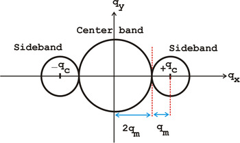
where “∝” means proportional since in the SIS-HOLZ, the interference occurs in the reciprocal space. The source separation is also in the reciprocal space and is equal to the split width. According to Eqs. (19) and (20), the wider the split HOLZ line, the finer the fringes. Furthermore, the lateral resolution or the maximum spatial frequency is determined by the fringe spacing of the interferogram. During the phase image reconstruction steps, to avoid the overlap between the center band and ± sidebands in the frequency space, the carrier frequency of fringes, q c, must be three times larger than q m. q m is the maximum spatial frequency in the frequency domain, Fig. 11. If the filter radius is smaller than 1/3q m, it will remove the phase information related to the strain. If it is larger than 1/3q m, the phase image will be complicated due to the noise contribution. It may carry some of the amplitude information from the center band.
A schematic of the frequency domain obtained by the FT of the interferogram. There is a center band and a side band. The carrier frequency of fringes must be at least three times larger than q m, to avoid overlapping the side bands and the center band. At least 3 fringes are required to reconstruct a phase image from an interferogram.

Therefore, the self-interference of a wider spit HOLZ lines gives finer fringes. However, not only a wide enough split HOLZ line is required but also the split needs to be symmetric in terms of intensity to satisfy
 ${a_{{\rm{g}}{{\rm{S}}_1}}} \cong {a_{{\rm{g}}{{\rm{S}}_2}}}$
[Eq. (14)].
The Gaussian filtering on the fringes before reconstruction helps to remove the background noise in the interferogram. This is suggested for very low interfering voltages, which are usually applied to fully self-interfere the smaller split widths. On the other hand, in 000 CBED disk, by moving the probe toward the Si/Si0.8Ge0.2 interface, the split width increases and the intensity of the split HOLZ line decreases due to the dynamical diffraction caused by the highly strained crystalline planes. Finally, at the interface and inside the superlattices, the split HOLZ line becomes fuzzy. Therefore, there is a trade off between choosing a wide and a symmetric split HOLZ line to have fine and high contrast fringes. This is seen in the 2D strain measurements performed by other researchers using the split width of HOLZ lines. Saitoh et al. Reference Saitoh, Yasuda, Hamabe and Tanaka11 started the strain measurements about 40 nm away from the interface and Clément et al. Reference Clément, Pantel, Kwakman and Rouvière12 could not measure the split width at <70 nm. So, the ROI is not at the interface of Si and Si0.8Ge0.2 but close to it inside the Si substrate. In this work, the aberration-corrected microscope helps to obtain the analyzable splits in 000 CBED disk even at ∼20 nm away from the interface.
Regardless of satisfying all calculation assumptions in the experiment, the calculated and the experimental profiles do not match perfectly. Two ends of the experimental and the calculated phase profiles do not follow the same trend which can be due to the residual effect of the biprism Fresnel fringes. In this technique, a reference phase profile from an interference pattern taken in the vacuum needs to be subtracted from the final obtained phase profile. The reference pattern helps to remove the Fresnel fringes and possible contamination on the biprism which can cause extra peaks in the phase profile. Additionally, in this work a clean area of the biprism is used to self-interfere the split HOLZ line. Likewise, the reflection g is considered parallel to the atomic displacement vector, R, however, if g is not parallel to R then |g.R| = |g||R| cos β, where β is an angle between the electron beam and the strained crystalline plane. Hence, the extra phase factor in Eq. (7) is exp(2π(gR) (cos β)), although the split width is still related to the displacement amplitude, R. Reference Saitoh, Yasuda, Hamabe and Tanaka11 This effect likely changes the phase profile symmetry.
By moving the probe on the specimen toward or away from the interface and by measuring the z-dependent displacement profile for 3 distinct split HOLZ lines, the 3D displacement profile can be obtained. However, not only there is a limit in moving toward the interface but also the distance away from the interface is limited. At areas farther from the interface, due to the lower strain, the split width decreases. Regarding Eqs. (19) and (20), both lower split width and lower biprism voltage increase the fringe spacing. Thicker fringes lead to the lower maximum spatial frequency, q m, which reduces the resolution. In the lower strained regions the SIS-HOLZ method needs lower biprism voltages to self-interfere the sources. So, theoretically, there is no limit in moving the probe and self-interfering various split width of HOLZ lines. Although, in practice, the decrease in the main peaks intensity near the interface and the small split width far from the interface limit the studying areas. In this work the ROI is limited roughly from 80 nm to 150 nm away from the interface.
Consequently, using an aberration-corrected TEM, choosing the right split width in terms of symmetry and intensity, aligning the biprism in the center of the split, adjusting the biprism defocus helps simplifying the exit diffracted wave calculations by removing the extra phase terms related to each. This gives a good agreement between the experimental and the calculated phase profiles.
VI. CONCLUSION
The novel SIS-HOLZ technique is applied on the split HOLZ line to self-interfere the main and internal intensities. This technique reconstructs the phase profile embedded inside the split HOLZ lines. The phase carries the z-dependent displacement information. The SIS-HOLZ analytical solution can be simplified by assuming a perfect overlap and removing the pre-field and post-field aberration terms. This is satisfied experimentally by using a spherical and coma aberration-corrected TEM. Although the biprism alignment and the spherical aberration play the dominant roles in simplifying the phase profile calculations, the symmetry and the width of the split HOLZ line, which contribute to the fringe spacing and contrast, need to be considered in the experiments. Correspondingly, the assumptions used in the simulation of the phase profile defined the limits of the experimental conditions to establish a good agreement between the experiment and the calculation. Future work will include, studying the effect of the biprism misalignment and different displacement profiles through the thickness of specimen.
ACKNOWLEDGMENT
NSERC support is greatly appreciated as is the help of Arthur Blackburn, Research Scientist of UVic’s Advanced Microscopy Facility.