1 Introduction
Nonlinear eigenvalue problems arise in many areas of computational science and engineering, including acoustics, control theory, fluid mechanics and structural engineering. The fundamental formulation of such problems is given in the following definition.
Definition 1.1. Given a non-empty open set
 $\unicode[STIX]{x1D6FA}\subseteq \mathbb{C}$
and a matrix-valued function
 $F:\unicode[STIX]{x1D6FA}\rightarrow \mathbb{C}^{n\times n}$
, the nonlinear eigenvalue problem (NEP) consists of finding scalars
 $\unicode[STIX]{x1D706}\in \unicode[STIX]{x1D6FA}$
(the eigenvalues) and nonzero vectors
 $v\in \mathbb{C}^{n}$
and
 $w\in \mathbb{C}^{n}$
(right and left eigenvectors) such that
 $$\begin{eqnarray}F(\unicode[STIX]{x1D706})v=0,\quad w^{\ast }F(\unicode[STIX]{x1D706})=0^{\ast }.\end{eqnarray}$$
Here
 $0$
denotes the zero column vector of
 $\mathbb{C}^{n}$
, and
 $(\cdot )^{\ast }$
denotes the conjugate transpose of a vector. We refer to
 $(\unicode[STIX]{x1D706},v)$
as an eigenpair of
 $F$
. The set of all eigenvalues is denoted by
 $\unicode[STIX]{x1D6EC}(F)$
and referred to as the spectrum of
 $F$
, while
 $\unicode[STIX]{x1D6FA}\setminus \unicode[STIX]{x1D6EC}(F)$
is called the resolvent set of
 $F$
.
Clearly, the eigenvalues
 $\unicode[STIX]{x1D706}$
of
 $F$
are the solutions of the scalar equation
 $f(z)=\det F(z)=0$
. The dependence of
 $F(z)$
on the parameter
 $z$
is typically nonlinear, giving the ‘N’ in NEP, but the eigenvectors enter the problem only linearly. Throughout this work we will denote by
 $z$
the parameter of
 $F$
as an independent variable, and we will use
 $\unicode[STIX]{x1D706}$
for the eigenvalues.
Three simple but representative examples of NEPs are listed below. We also give links to corresponding problems in the NLEVP collection by Betcke et al. (Reference Betcke, Higham, Mehrmann, Schröder and Tisseur2013). We will use some of these problems later on for numerical illustrations.
-
(i) Stability analysis of delay differential equations (DDEs). Consider the linear first-order homogeneous DDE
(1.1)Solutions of the form $$\begin{eqnarray}u^{\prime }(t)+Au(t)+Bu(t-1)=0,\quad u(t)~\text{given for}~t\in [-1,0].\end{eqnarray}$$
$u(t)=\text{e}^{\unicode[STIX]{x1D706}t}v$
can be obtained from the NEP and the real parts of the eigenvalues
$$\begin{eqnarray}F(\unicode[STIX]{x1D706})v=(\unicode[STIX]{x1D706}I+A+B\,\text{e}^{-\unicode[STIX]{x1D706}})v=0,\end{eqnarray}$$
$\unicode[STIX]{x1D706}$
determine the growth of
$\Vert u\Vert =\text{e}^{t\,\text{Re}\unicode[STIX]{x1D706}}\Vert v\Vert$
. A problem of this type is part of the NLEVP collection under the name time_delay. Detailed expositions of the stability theory of time-delay systems can be found in Gu, Kharitonov and Chen (Reference Gu, Kharitonov and Chen2003) and Michiels and Niculescu (Reference Michiels and Niculescu2007).
-
(ii) Differential equations with nonlinear boundary conditions. A minimal example from Solov’ëv (Reference Solov’ëv2006) is a boundary value problem on
$[0,1]$
, (1.2)Upon applying a finite element discretization with linear hat functions centred at the equispaced points
$$\begin{eqnarray}-u^{\prime \prime }(x)=\unicode[STIX]{x1D706}u(x),\quad u(0)=0,\quad -u^{\prime }(1)=\unicode[STIX]{x1D719}(\unicode[STIX]{x1D706})u(1).\end{eqnarray}$$
$x_{i}=i/n$
(
$i=1,2,\ldots ,n$
), (1.2) can be rewritten as an NEP, (1.3)with
$$\begin{eqnarray}F(\unicode[STIX]{x1D706})u=(C_{1}-\unicode[STIX]{x1D706}C_{2}+\unicode[STIX]{x1D719}(\unicode[STIX]{x1D706})C_{3})u=0\end{eqnarray}$$
$n\times n$
matrices and
$$\begin{eqnarray}C_{1}=n\left[\begin{array}{@{}cccc@{}}2 & -1\\ -1 & \ddots & \ddots \\ & \ddots & 2 & -1\\ & & -1 & 1\end{array}\right]\!,~~C_{2}=\frac{1}{6n}\left[\begin{array}{@{}cccc@{}}4 & 1\\ 1 & \ddots & \ddots \\ & \ddots & 4 & 1\\ & & 1 & 2\end{array}\right]\!,~~C_{3}=e_{n}^{}e_{n}^{T},\end{eqnarray}$$
$e_{n}=[0,\ldots ,0,1]^{T}$
. With the rational function
$\unicode[STIX]{x1D719}(\unicode[STIX]{x1D706})=\unicode[STIX]{x1D706}/(\unicode[STIX]{x1D706}-1)$
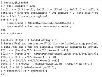
, this problem is contained in the NLEVP collection under the name loaded_string.
A property that is common to many NEPs is that the nonlinearity appears only in a few entries of
$F(z)$
. Indeed, the nonlinearity in this example affects only a single entry through the rank-1 matrix
$C_{3}$
. This low-rank structure is typically worth exploiting. -
(iii) Transparent boundary conditions. This is a special case of (b), where the right boundary condition is chosen so that (1.2) is satisfied on an interval larger than the discretization interval, e.g. for all
$x\in [0,+\infty )$
. Note that the solutions of (1.2) on
$[0,+\infty )$
are of the form Therefore, in order to model a ‘transparent’ boundary, the Dirichlet-to-Neumann map
$$\begin{eqnarray}u(x)=\unicode[STIX]{x1D6FC}\sin (\sqrt{\unicode[STIX]{x1D706}}x).\end{eqnarray}$$
$\unicode[STIX]{x1D719}$
at
$x=1$
should satisfy Problems with similar types of nonlinearities are encountered, for example, with the modelling of waveguides. The gun problem available in the NLEVP collection,
$$\begin{eqnarray}\unicode[STIX]{x1D719}(\unicode[STIX]{x1D706})=-\frac{\sqrt{\unicode[STIX]{x1D706}}}{\tan (\sqrt{\unicode[STIX]{x1D706}})}.\end{eqnarray}$$
(1.4)models a waveguide-loaded accelerator cavity with the values of
$$\begin{eqnarray}F(\unicode[STIX]{x1D706})v=\Bigl(K-\unicode[STIX]{x1D706}M+\text{i}\sqrt{\unicode[STIX]{x1D706}-\unicode[STIX]{x1D714}_{1}^{2}}\,W_{1}+\text{i}\sqrt{\unicode[STIX]{x1D706}-\unicode[STIX]{x1D714}_{2}^{2}}\,W_{2}\Bigr)v=0,\end{eqnarray}$$
$\unicode[STIX]{x1D714}_{j}$
corresponding to cut-off wave numbers of modes in two waveguide ports. Here
$M$
,
$K$
,
$W_{1}$
and
$W_{2}$
are real symmetric
$9956\times 9956$
matrices arising from the finite element discretization of Maxwell’s equation for the electric field
$$\begin{eqnarray}\unicode[STIX]{x1D6FB}\times \biggl(\displaystyle \frac{1}{\unicode[STIX]{x1D707}}\unicode[STIX]{x1D6FB}\times E\biggr)-\unicode[STIX]{x1D706}\unicode[STIX]{x1D716}E=0\end{eqnarray}$$
$E$
on some spatial domain; see Liao, Bai, Lee and Ko (Reference Liao, Bai, Lee and Ko2010) for details. Also in this example the matrices
$W_{1}$
and
$W_{2}$
associated with the waveguide boundaries are of low rank.






For an exposition of other interesting applications where NEPs arise, we refer to the introductory chapters of the PhD theses by Effenberger (Reference Effenberger2013a
) and Van Beeumen (Reference Van Beeumen2015). Note that, independent of a particular application, NEPs are of mathematical interest as systems of nonlinear equations, or scalar root-finding problems, e.g. for
 $f(z)=\det F(z)$
.
There are also problems for which
 $F$
does not depend on
 $z$
but depends instead on the eigenvectors or a selection of eigenvectors, with applications in electronic structure calculations (Saad et al.
Reference Saad, Stathopoulos, Chelikowsky, Wu and Öğüt1996), machine learning (Bühler and Hein Reference Bühler and Hein2009), and even for the ranking of football teams (Keener Reference Keener1993). Formally, these eigenvalue problems consist of finding nontrivial solutions of
 $F(V)V=VD$
, where
 $F$
is an
 $n\times n$
matrix that depends on an
 $n\times k$
matrix of eigenvectors
 $V$
, and
 $D$
is a
 $k\times k$
diagonal matrix containing the corresponding eigenvalues. This type of nonlinear dependency will not be considered here. Another interesting class is that of multi-parameter NEPs
 $F(\unicode[STIX]{x1D706},\unicode[STIX]{x1D6FE})v=0$
which arise, for example, in the stability analysis of parametrized nonlinear wave equations (Beyn and Thümmler Reference Beyn and Thümmler2009) and the delay-independent stability analysis of DDEs (Gu et al.
Reference Gu, Kharitonov and Chen2003, Chapter 4.6). Although we will not discuss multi-parameter NEPs in this survey any further, continuation methods for their solution typically require solving an NEP as in Definition 1.1 at every iteration.
Our aim is to survey NEPs through their interesting mathematical properties and numerical solution techniques. While we mention and list some applications where NEPs arise, these are not our main focus. We hope that this survey will be useful for mathematicians, computational scientists and engineers alike. Those new to the field may want to learn first about the basic mathematical properties of NEPs, such as their solution structure and the sensitivity of eigenvalues, and Section 2 should be a good starting point for that. We also provide an extensive list of references for further exploration, although we do not claim that this is a complete list for this very rich and rapidly developing area. Practitioners who already have a concrete NEP to solve can use this survey to get an overview of available solution techniques. To facilitate choosing the right method, we highlight the guiding principles and various problems that come with each numerical method such as, for example, the selection of suitable parameters.
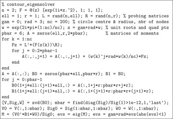
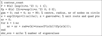
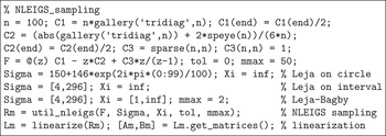
With practical solution methods being the main focus, and to make this survey more interactive, we include several MATLAB code snippets. Some of the snippets require MATLAB R2016b or later, because they use local functions in a script (Higham and Higham Reference Higham and Higham2017). The codes are also available online at
http://www.maths.manchester.ac.uk/nep/
We encourage the reader to execute them in MATLAB and play with the parameters. Most of the codes also run with little or no modification in GNU Octave (Eaton, Bateman, Hauberg and Wehbring Reference Eaton, Bateman, Hauberg and Wehbring2016). We emphasize that our code snippets should not be considered as full implementations of robust numerical methods! They merely serve the purpose of illustration.
In addition to the codes, the above website also contains the bibliography of this survey, as well as an up-to-date list of links to available NEP-related software. Alongside this survey, the reader is encouraged to consult the review by Mehrmann and Voss (Reference Mehrmann and Voss2004), which discusses many NEP applications and describes some of the methods contained here (but not, for example, the contour-based and rational interpolation-based solvers developed since 2004). Quadratic eigenvalue problems are reviewed in detail by Tisseur and Meerbergen (Reference Tisseur and Meerbergen2001). For quadratic and more generally polynomial eigenvalue problems, the exploitation of special structure in the coefficient matrices is well researched; see for example Mackey, Mackey, Mehl and Mehrmann (Reference Mackey, Mackey, Mehl and Mehrmann2006a ), Mackey, Mackey and Tisseur (Reference Mackey, Mackey, Tisseur and Benner2015) and the references therein. In our discussions of NEPs with special structure we will restrict our attention to the Hermitian case (see Section 3) and problems with low-rank structure. Hermitian NEPs are the most frequently encountered in practice and by far the best understood. The exploitation of low-rank structure in NEPs often leads to considerable computational savings.
The outline of this work is as follows. Section 2 provides an overview of the solution structure of NEPs, including discussions of root functions and invariant pairs, the Smith form and Keldysh’s theorem, and generalized Rayleigh functionals, as well as some perturbation results. The short Section 3 is devoted to Hermitian NEPs. Sections 4, 5 and 6 are on numerical methods. Section 4 is about NEP solvers based on Newton’s method, with particular attention paid to relating the various existing methods and illustrating their convergence properties with examples. Section 5 is devoted to NEP solvers using contour integrals. Here again our main focus is on summarizing and relating existing algorithms, as well as discussing their dependence on parameters. Section 6 gives an overview of solution methods based on the linearization of rational eigenvalue problems. Here our focus is on the practical and efficient construction of rational interpolants via sampling of the matrix-valued function defining an NEP. Each of the sections on numerical methods ends with a brief overview of existing software, giving links to online resources whenever possible.
Within the sections of this paper we use common counters in the numbering of definitions, theorems, algorithms, figures, etc. We believe this simplifies referencing for the reader since, for example, locating Remark 2.2 tells one that a definition with number 2.3 should follow. Subsections and equations are enumerated separately within each section.
2 Solution structure of NEPs
In this section we will shed light on the solution structure of NEPs. As the examples in this section aim to illustrate, the solution properties of general NEPs are quite different from linear eigenvalue problems
 $Av=\unicode[STIX]{x1D706}v$
, where
 $A\in \mathbb{C}^{n\times n}$
and
 $0\neq v\in \mathbb{C}^{n}$
, although such problems are special cases of NEPs with
 $F(z)=A-zI$
. Nevertheless, we will see that with an appropriate definition of eigenvalue multiplicity and generalized eigenvectors, a rather elegant characterization of NEP solutions can be obtained. Much of the theory we review here can be found in the monograph by Mennicken and Möller (Reference Mennicken and Möller2003), therein developed in more detail and greater generality for operator functions in Banach spaces. The appendix of the monograph by Kozlov and Maz’ja (Reference Kozlov and Maz’ja1999) also contains a good summary of parts of the theory, including a complete proof of Keldysh’s theorem. A collection of mathematical facts about NEPs is given by Voss (Reference Voss and Hogben2014).
2.1 Eigenvalues and eigenvectors
To develop our intuition about the eigenvalue structure of NEPs, it will be instructive to first think of a scalar function
 $F:\unicode[STIX]{x1D6FA}\rightarrow \mathbb{C}$
. The associated NEP
 $F(\unicode[STIX]{x1D706})v=0$
,
 $v\neq 0$
, is just a scalar root-finding problem. It becomes immediately apparent that an NEP on
 $\unicode[STIX]{x1D6FA}=\mathbb{C}$
may have
-
∙ no solutions at all, e.g. if
$F(z)=\exp (z)$
, -
∙ finitely many solutions, e.g. if
$F(z)=z^{3}-1$
, -
∙ infinitely many solutions, e.g. if
$F(z)=\cos (z)$
.


The fact that even an NEP of size
 $1\times 1$
can have more than one eigenvalue tells us that the eigenvectors belonging to distinct eigenvalues need not be linearly independent: indeed the ‘vector’
 $v=[\,1\,]$
is an eigenvector for all eigenvalues of an
 $1\times 1$
NEP. An example of size
 $2\times 2$
is
 $$\begin{eqnarray}F(z)=\left[\begin{array}{@{}cc@{}}\text{e}^{\text{i}z^{2}} & 1\\ 1 & 1\end{array}\right]\!,\end{eqnarray}$$
which is a singular matrix exactly at the points
 $z\in \mathbb{C}$
where
 $\text{e}^{\text{i}z^{2}}=1$
. Hence the eigenvalues of
 $F$
are
 $\unicode[STIX]{x1D706}_{k}=\pm \sqrt{2\unicode[STIX]{x1D70B}k}$
(
 $k=0,\pm 1,\pm 2,\ldots$
) and
 $[{1\atop -1}]$
is a right and left eigenvector for all of them. It will be useful to keep the function
 $F$
defined by (2.1) in mind as we will often refer back to it for illustration.
In the following discussions we will assume that
 $F:\unicode[STIX]{x1D6FA}\rightarrow \mathbb{C}^{n\times n}$
is holomorphic in a connected open set
 $\unicode[STIX]{x1D6FA}\subseteq \mathbb{C}$
(the domain), denoted by
 $F\in H(\unicode[STIX]{x1D6FA},\mathbb{C}^{n\times n})$
. This assumption is satisfied for most NEPs encountered in practice, where the elements of
 $F(z)$
are usually polynomial, rational, algebraic or exponential functions of
 $z\in \unicode[STIX]{x1D6FA}$
, or a combination thereof. As the definition of a matrix determinant involves only finite sums and products of the matrix entries,
 $F\in H(\unicode[STIX]{x1D6FA},\mathbb{C}^{n\times n})$
also implies that
 $\det F(z)\in H(\unicode[STIX]{x1D6FA},\mathbb{C})$
. Hence the eigenvalues of
 $F$
are the roots of a scalar holomorphic function in the domain
 $\unicode[STIX]{x1D6FA}$
. The following discreteness result is a consequence of that and can be found, for example, in Mennicken and Möller (Reference Mennicken and Möller2003, Theorem 1.3.1).
Theorem 2.1. Let
 $\unicode[STIX]{x1D6FA}\subseteq \mathbb{C}$
be a domain and
 $F\in H(\unicode[STIX]{x1D6FA},\mathbb{C}^{n\times n})$
. Then the resolvent set
 $\unicode[STIX]{x1D6FA}\setminus \unicode[STIX]{x1D6EC}(F)$
is open. If the resolvent set is non-empty, every eigenvalue
 $\unicode[STIX]{x1D706}\in \unicode[STIX]{x1D6EC}(F)$
is isolated, that is, there exists an open neighbourhood
 ${\mathcal{U}}\subset \unicode[STIX]{x1D6FA}$
such that
 ${\mathcal{U}}\cap \unicode[STIX]{x1D6EC}(F)=\{\unicode[STIX]{x1D706}\}$
.
The condition that the resolvent set be non-empty is equivalent to saying that
 $\det F(z)$
does not vanish identically on
 $\unicode[STIX]{x1D6FA}$
. In this case we say that
 $F$
is regular. While a regular
 $F$
can have an infinite number of eigenvalues in
 $\unicode[STIX]{x1D6FA}$
, the set of eigenvalues
 $\unicode[STIX]{x1D6EC}(F)$
does not have accumulation points in
 $\unicode[STIX]{x1D6FA}$
. An illustrating example is the scalar function
 $F(z)=\sin (1/z)$
, which is holomorphic in
 $\unicode[STIX]{x1D6FA}=\mathbb{C}\setminus \{0\}$
with an infinite number of roots accumulating at
 $0\not \in \unicode[STIX]{x1D6FA}$
.
The algebraic multiplicity of an eigenvalue
 $\unicode[STIX]{x1D706}$
is defined as the multiplicity of the root of
 $\det F(z)$
at
 $z=\unicode[STIX]{x1D706}$
, that is, the smallest integer
 $j\geq 1$
such that
 $$\begin{eqnarray}\frac{\text{d}^{j}}{\text{d}z^{j}}\,\det F(z)\Big|_{z=\unicode[STIX]{x1D706}}\neq 0.\end{eqnarray}$$
The algebraic multiplicity of an isolated eigenvalue must be finite, but in contrast to linear eigenvalue problems, in the nonlinear case the algebraic multiplicity of an eigenvalue is not necessarily bounded by the problem size
 $n$
. This is illustrated by the scalar example
 $F(z)=z^{n+1}$
, which has the eigenvalue
 $\unicode[STIX]{x1D706}=0$
of algebraic multiplicity
 $n+1$
.
By Definition 1.1, the right eigenvectors associated with an eigenvalue
 $\unicode[STIX]{x1D706}$
are the nonzero vectors in the null space of
 $F(\unicode[STIX]{x1D706})$
, denoted by
 $\operatorname{null}F(\unicode[STIX]{x1D706})$
. The dimension of this null space,
 $\dim (\operatorname{null}F(\unicode[STIX]{x1D706}))$
, is called the geometric multiplicity of
 $\unicode[STIX]{x1D706}$
. An eigenvalue
 $\unicode[STIX]{x1D706}$
is called semisimple if its geometric multiplicity is equal to its algebraic multiplicity, and it is called simple if its algebraic multiplicity equals one.
Remark 2.2. In some cases it is of interest to consider NEPs with eigenvalues at infinity, for example in the stability analysis of linear time-invariant delay differential-algebraic equations (Du, Linh, Mehrmann and Thuan Reference Du, Linh, Mehrmann and Thuan2013) or when deflating already computed eigenvalues (see Section 4.3). We say that
 $F:\unicode[STIX]{x1D6FA}\rightarrow \mathbb{C}^{n\times n}$
defined on
 $\unicode[STIX]{x1D6FA}\subseteq \overline{\mathbb{C}}:=\mathbb{C}\cup \{\infty \}$
with
 $\infty \in \unicode[STIX]{x1D6FA}$
has an eigenvalue at
 $\unicode[STIX]{x1D706}=\infty$
if
 $$\begin{eqnarray}G:z\mapsto F(1/z)\end{eqnarray}$$
has an eigenvalue at
 $z=0$
. The algebraic and geometric multiplicities of
 $\unicode[STIX]{x1D706}=\infty$
in
 $F$
are simply defined as the corresponding algebraic and geometric multiplicities of
 $z=0$
in
 $G$
. Indeed, if an NEP is considered on the extended complex plane
 $\overline{\mathbb{C}}$
instead of
 $\mathbb{C}$
, the point
 $z=\infty$
is not more or less distinguished than any other complex number. In particular, the point at infinity can always be mapped to a finite point via a Möbius transformation. Hence there is no need to further discuss infinite eigenvalues of NEPs separately.
Note that our definition of eigenvalues at infinity is not in contradiction to the common definition of infinite eigenvalues for matrix polynomials
 $P(z)=\sum _{j=0}^{\ell }z^{j}C_{j}$
,
 $C_{\ell }\neq O$
, as the zero eigenvalues of the reversal matrix polynomial
 $z^{\ell }P(1/z)$
. When considered as an NEP in the sense used here, the function
 $P$
is actually not well defined at
 $z=\infty$
. Hence the convention is to instead consider the function
 $F(z)=z^{-\ell }P(z)$
, which is well defined (and even holomorphic) at
 $z=\infty$
and so it makes sense to consider eigenvalues there. Indeed,
 $G(z)=F(1/z)$
is the reversal of
 $P$
.
2.2 Root functions and generalized eigenvectors
An elegant definition of generalized eigenvectors is based on root functions, a concept introduced by Trofimov (Reference Trofimov1968). To motivate the idea of root functions, it is helpful to first consider a linear eigenvalue problem
 $Av=\unicode[STIX]{x1D706}v$
for
 $A\in \mathbb{C}^{n\times n}$
and
 $0\neq v\in \mathbb{C}^{n}$
, and to recall from matrix analysis that a sequence
 $(v_{0},v_{1},\ldots ,v_{m-1})$
of nonzero vectors is called a Jordan chain for the eigenvalue
 $\unicode[STIX]{x1D706}$
if
 $$\begin{eqnarray}(A-\unicode[STIX]{x1D706}I)v_{0}=0,\quad (A-\unicode[STIX]{x1D706}I)v_{1}=v_{0},~\ldots ,~(A-\unicode[STIX]{x1D706}I)v_{m-1}=v_{m-2};\end{eqnarray}$$
see, for example, the monograph by Horn and Johnson (Reference Horn and Johnson1985, Chapter 3). The vector
 $v_{0}$
is a right eigenvector of
 $A$
, or equivalently, a nonzero right null vector of
 $A-\unicode[STIX]{x1D706}I$
, and the
 $v_{0},v_{1},\ldots ,v_{m-1}$
are generalized eigenvectors of
 $A$
. Generalized eigenvectors of a matrix can be easily seen to be linearly independent. The maximal length
 $m$
of a Jordan chain starting with
 $v_{0}$
is called the rank of
 $v_{0}$
.
Interestingly, by defining the functions
 $v(z)=\sum _{j=0}^{m-1}(z-\unicode[STIX]{x1D706})^{j}v_{j}$
and
 $F(z)=A-zI$
, the
 $m$
equations in (2.2) can be rewritten as
 $$\begin{eqnarray}\frac{\text{d}^{j}}{\text{d}z^{j}}\,F(z)v(z)\Big|_{z=\unicode[STIX]{x1D706}}=j!\mathop{\sum }_{k=0}^{j}\frac{F^{(k)}(\unicode[STIX]{x1D706})}{k!}v_{j-k}=0,\quad j=0,1,\ldots ,m-1,\end{eqnarray}$$
where
 $F^{(k)}(z)={\textstyle \frac{\text{d}^{k}}{\text{d}z^{k}}}F(z)$
. In other words,
 $F(z)v(z)$
has a root of multiplicity at least
 $m$
at
 $z=\unicode[STIX]{x1D706}$
. While (2.2) is specific to linear eigenvalue problems, (2.3) extends straightforwardly to the nonlinear case. The main difference for NEPs is that generalized eigenvectors need not necessarily be linearly independent, and even the zero vector is admitted as a generalized eigenvector. We make this precise in the following definition, which has been adopted from Mennicken and Möller (Reference Mennicken and Möller2003, Definition 1.6.1).
Definition 2.3. Let
 $F\in H(\unicode[STIX]{x1D6FA},\mathbb{C}^{n\times n})$
be regular on a non-empty domain
 $\unicode[STIX]{x1D6FA}\subseteq \mathbb{C}$
, and let
 $\unicode[STIX]{x1D706}\in \unicode[STIX]{x1D6FA}$
be given.
-
(i) A holomorphic vector-valued function
$v\in H(\unicode[STIX]{x1D6FA},\mathbb{C}^{n})$
such that
$v(\unicode[STIX]{x1D706})\neq 0$
and
$F(\unicode[STIX]{x1D706})v(\unicode[STIX]{x1D706})=0$
is called a root function for
$F$
at
$\unicode[STIX]{x1D706}$
. The multiplicity of the root
$z=\unicode[STIX]{x1D706}$
of
$F(z)v(z)$
is denoted by
$s(v)$
. -
(ii) A tuple
$(v_{0},v_{1},\ldots ,v_{m-1})\in (\mathbb{C}^{n})^{m}$
with
$m\geq 1$
and
$v_{0}\neq 0$
is called a Jordan chain for
$F$
at
$\unicode[STIX]{x1D706}$
if is a root function for
$$\begin{eqnarray}v(z)=\mathop{\sum }_{k=0}^{m-1}(z-\unicode[STIX]{x1D706})^{k}v_{k}\end{eqnarray}$$
$F$
at
$\unicode[STIX]{x1D706}$
and
$s(v)\geq m$
.
-
(iii) For a given vector
$v_{0}\in \operatorname{null}F(\unicode[STIX]{x1D706})\setminus \{0\}$
, the number is called the rank of
$$\begin{eqnarray}r(v_{0})=\max \{s(v):v\text{ is a root function for }F\text{ at }\unicode[STIX]{x1D706}\text{ with }v(\unicode[STIX]{x1D706})=v_{0}\}\end{eqnarray}$$
$v_{0}$
.
-
(iv) A system of vectors in
$\mathbb{C}^{n}$
, is a complete system of Jordan chains for
$$\begin{eqnarray}V=(v_{k}^{j}:0\leq k\leq m_{j}-1,~1\leq j\leq d),\end{eqnarray}$$
$F$
at
$\unicode[STIX]{x1D706}$
if-
(a)
$d=\dim (\operatorname{null}F(\unicode[STIX]{x1D706}))$
and
$\{v_{0}^{1},v_{0}^{2},\ldots ,v_{0}^{d}\}$
is a basis of
$\operatorname{null}F(\unicode[STIX]{x1D706})$
, -
(b) the tuple
$(v_{0}^{j},v_{1}^{j},\ldots ,v_{m_{j}-1}^{j})$
is a Jordan chain for
$F$
at
$\unicode[STIX]{x1D706}$
for
$j=1,2,\ldots ,d$
, -
(c)
$m_{j}=\max \{r(v_{0}):v_{0}\in \operatorname{null}F(\unicode[STIX]{x1D706})\setminus \operatorname{span}\{v_{0}^{\unicode[STIX]{x1D708}}:1\leq \unicode[STIX]{x1D708}<j\}\}$
for
$j=1,2,\ldots ,d$
.
-










It can be shown (Mennicken and Möller Reference Mennicken and Möller2003, Proposition 1.6.4) that a complete system of Jordan chains always exists, which essentially requires the verification that for a regular NEP the rank
 $r(v_{0})$
of any eigenvector
 $v_{0}$
is finite. The numbers
 $m_{j}$
satisfy
 $m_{1}\geq m_{2}\geq \cdots \geq m_{d}$
by definition and are called the partial multiplicities of
 $\unicode[STIX]{x1D706}$
. It can be shown that
 $\sum _{j=1}^{d}m_{j}$
corresponds to the algebraic multiplicity of
 $\unicode[STIX]{x1D706}$
(Mennicken and Möller Reference Mennicken and Möller2003, Proposition 1.8.5). The number
 $m_{1}$
is called the index of
 $\unicode[STIX]{x1D706}$
. If
 $m_{1}=\cdots =m_{d}=1$
, then
 $\unicode[STIX]{x1D706}$
is a semisimple eigenvalue; if in addition
 $d=1$
, then
 $\unicode[STIX]{x1D706}$
is a simple eigenvalue.
Example 2.4. Consider the
 $2\times 2$
function
 $F$
defined in (2.1). The eigenvalue
 $\unicode[STIX]{x1D706}_{0}=0$
has algebraic multiplicity two and geometric multiplicity one. The corresponding right eigenvector
 $v_{0}$
and generalized eigenvector
 $v_{1}$
are both multiples of
 $[{1\atop -1}]$
, and hence are not linearly independent. The vector-valued function
 $v(z)=v_{0}+zv_{1}=[{1+z\atop -1-z}]$
is a root function for
 $F$
at
 $\unicode[STIX]{x1D706}_{0}=0$
, and the multiplicity of
 $\unicode[STIX]{x1D706}_{0}$
as a root of
 $F(z)v(z)$
can be easily shown to be
 $s(v)=2$
. Using the MATLAB Symbolic Math Toolbox we find that
 ${\textstyle \frac{\text{d}^{2}}{\text{d}z^{2}}}F(z)v(z)$
is the smallest-order derivative which does not vanish at
 $z=0$
:

Hence the rank of the right eigenvector
 $v_{0}$
with eigenvalue
 $\unicode[STIX]{x1D706}_{0}$
is
 $r(v_{0})\geq 2$
, but since
 $\unicode[STIX]{x1D706}_{0}$
has algebraic multiplicity two,
 $r(v_{0})=2$
. The pair
 $([{1\atop -1}],[{1\atop -1}])$
is a Jordan chain for
 $F$
at
 $\unicode[STIX]{x1D706}_{0}=0$
, and also a complete system of Jordan chains there.
So far we have only considered right eigenvectors of
 $F$
, but clearly left eigenvectors of
 $F$
can be obtained as the right eigenvectors of
 $F^{\ast }$
. It turns out that there is a natural way to complement a complete system of Jordan chains for
 $F$
at
 $\unicode[STIX]{x1D706}$
with a complete system of Jordan chains of
 $F^{\ast }$
at
 $\unicode[STIX]{x1D706}$
, and the latter is uniquely determined if certain normalization conditions are enforced. The following result makes this precise (Mennicken and Möller Reference Mennicken and Möller2003, Theorem 1.6.5).
Theorem 2.5. Let
 $F\in H(\unicode[STIX]{x1D6FA},\mathbb{C}^{n\times n})$
be regular on a non-empty domain
 $\unicode[STIX]{x1D6FA}\subseteq \mathbb{C}$
, and consider an eigenvalue
 $\unicode[STIX]{x1D706}\in \unicode[STIX]{x1D6EC}(F)$
. Let
 $$\begin{eqnarray}V=(v_{k}^{j}:0\leq k\leq m_{j}-1,~1\leq j\leq d)\end{eqnarray}$$
be a complete system of Jordan chains for
 $F$
at
 $\unicode[STIX]{x1D706}$
. Then there exists a unique complete system of Jordan chains
 $$\begin{eqnarray}W=(w_{k}^{j}:0\leq k\leq m_{j}-1,~1\leq j\leq d)\end{eqnarray}$$
for
 $F^{\ast }$
at
 $\unicode[STIX]{x1D706}$
such that each eigenvector
 $w_{0}^{j}$
has rank
 $r(w_{0}^{j})=m_{j}$
and
 $$\begin{eqnarray}\mathop{\sum }_{\unicode[STIX]{x1D6FC}=0}^{k}\mathop{\sum }_{\unicode[STIX]{x1D6FD}=1}^{m_{i}}w_{k-\unicode[STIX]{x1D6FC}}^{j\ast }\frac{F^{(\unicode[STIX]{x1D6FC}+\unicode[STIX]{x1D6FD})}(\unicode[STIX]{x1D706})}{(\unicode[STIX]{x1D6FC}+\unicode[STIX]{x1D6FD})!}v_{m_{i}-\unicode[STIX]{x1D6FD}}^{i}=\unicode[STIX]{x1D6FF}_{ij}\unicode[STIX]{x1D6FF}_{0k},\quad 0\leq k\leq m_{j}-1,~1\leq i,j\leq d,\end{eqnarray}$$
with the Kronecker delta
 $$\begin{eqnarray}\unicode[STIX]{x1D6FF}_{ij}=\left\{\begin{array}{@{}ll@{}}0\quad & \text{if }i\neq j,\\ 1\quad & \text{if }i=j.\end{array}\right.\end{eqnarray}$$
Example 2.6. Consider the matrix-valued function
 $F$
in (2.1). We found in Example 2.4 that the pair
 $$\begin{eqnarray}V=(v_{0},v_{1})=\biggl(\biggl[{1\atop -1}\biggr],\biggl[{1\atop -1}\biggr]\biggr)\end{eqnarray}$$
is a complete system of Jordan chains for
 $F$
at
 $\unicode[STIX]{x1D706}=0$
. A similar construction shows that
 $$\begin{eqnarray}W=(w_{0},w_{1})=\biggl(\unicode[STIX]{x1D70C}_{0}\biggl[{1\atop -1}\biggr],\unicode[STIX]{x1D70C}_{1}\biggl[{1\atop -1}\biggr]\biggr)\quad \text{with }\unicode[STIX]{x1D70C}_{0},\unicode[STIX]{x1D70C}_{1}\in \mathbb{C}\setminus \{0\}\end{eqnarray}$$
is a complete system of Jordan chains for
 $F^{\ast }$
at
 $\unicode[STIX]{x1D706}=0$
satisfying
 $r(w_{0})=2$
. The normalization conditions (2.4) become
 $$\begin{eqnarray}\displaystyle w_{0}^{\ast }F^{\prime }(0)v_{1}+w_{0}^{\ast }\frac{F^{\prime \prime }(0)}{2}v_{0} & = & \displaystyle 1,\nonumber\\ \displaystyle w_{1}^{\ast }F^{\prime }(0)v_{1}+w_{1}^{\ast }\frac{F^{\prime \prime }(0)}{2}v_{0}+w_{0}^{\ast }\frac{F^{\prime \prime }(0)}{2}v_{1}+w_{0}^{\ast }\frac{F^{\prime \prime \prime }(0)}{6}v_{0} & = & \displaystyle 0,\nonumber\end{eqnarray}$$
and they are satisfied if we choose
 $\unicode[STIX]{x1D70C}_{0}=\text{i}$
and
 $\unicode[STIX]{x1D70C}_{1}=-\text{i}$
.
While the normalization conditions in Theorem 2.5 look rather messy in general, they simplify if the eigenvalue
 $\unicode[STIX]{x1D706}$
is semisimple. In this case we have
 $m_{1}=\cdots =m_{d}=1$
so that (2.4) becomes
 $$\begin{eqnarray}w_{0}^{j\ast }F^{\prime }(\unicode[STIX]{x1D706})v_{0}^{i}=\unicode[STIX]{x1D6FF}_{ij},\quad 1\leq i,j\leq d,\end{eqnarray}$$
that is, the left and right eigenvectors can be chosen
 $F^{\prime }(\unicode[STIX]{x1D706})$
-biorthonormal.
2.3 Factorizations: Smith form
It is often useful to have a factorization of an NEP about one or multiple eigenvalues, giving rise to local or global factorizations, respectively. A very useful factorization is the so-called Smith form, which we state in its global version; see Leiterer (Reference Leiterer1978), Gohberg and Rodman (Reference Gohberg and Rodman1981) and Kozlov and Maz’ja (Reference Kozlov and Maz’ja1999, Chapter A.6). It uses the notion of a unimodular matrix-valued function
 $P\in H(\unicode[STIX]{x1D6FA},\mathbb{C}^{n\times n})$
, which means that
 $\det P(z)$
is a nonzero constant over
 $\unicode[STIX]{x1D6FA}$
.
Theorem 2.7 (Smith form).
Let
 $F\in H(\unicode[STIX]{x1D6FA},\mathbb{C}^{n\times n})$
be regular on a non-empty domain
 $\unicode[STIX]{x1D6FA}$
. Let
 $\unicode[STIX]{x1D706}_{i}$
(
 $i=1,2,\ldots$
) be the distinct eigenvalues of
 $F$
in
 $\unicode[STIX]{x1D6FA}$
with partial multiplicities
 $m_{i,1}\geq m_{i,2}\geq \cdots \geq m_{i,d_{i}}$
. Then there exists a global Smith form
 $$\begin{eqnarray}P(z)F(z)Q(z)=D(z),\quad z\in \unicode[STIX]{x1D6FA},\end{eqnarray}$$
with unimodular matrix-valued functions
 $P,Q\in H(\unicode[STIX]{x1D6FA},\mathbb{C}^{n\times n})$
, and
 $$\begin{eqnarray}D(z)=\operatorname{diag}(\unicode[STIX]{x1D6FF}_{1}(z),\unicode[STIX]{x1D6FF}_{2}(z),\ldots ,\unicode[STIX]{x1D6FF}_{n}(z)).\end{eqnarray}$$
The diagonal entries
 $\unicode[STIX]{x1D6FF}_{j}$
are of the form
 $$\begin{eqnarray}\unicode[STIX]{x1D6FF}_{j}(z)=h_{j}(z)\mathop{\prod }_{i=1,2,\ldots }(z-\unicode[STIX]{x1D706}_{i})^{m_{i,j}},\quad j=1,\ldots ,n,\end{eqnarray}$$
where
 $m_{i,j}=0$
if
 $j>d_{i}$
and each
 $h_{j}\in H(\unicode[STIX]{x1D6FA},\mathbb{C})$
is free of roots on
 $\unicode[STIX]{x1D6FA}$
.
From the Smith form it is easy to identify eigenvectors of
 $F$
for an eigenvalue
 $\unicode[STIX]{x1D706}_{i}$
. Let
 $Q$
be partitioned columnwise as
 $Q(z)=[q_{1}(z),q_{2}(z),\ldots ,q_{n}(z)].$
By the diagonal structure of
 $D$
, the canonical unit vectors
 $e_{1},e_{2},\ldots ,e_{d_{i}}$
form a basis of
 $\operatorname{null}D(\unicode[STIX]{x1D706}_{i})$
, and therefore also a basis of
 $\operatorname{null}(P(\unicode[STIX]{x1D706}_{i})F(\unicode[STIX]{x1D706}_{i})Q(\unicode[STIX]{x1D706}_{i}))$
. Hence we have found a basis of
 $d_{i}$
right eigenvectors of
 $F$
for
 $\unicode[STIX]{x1D706}$
, namely,
 $$\begin{eqnarray}q_{1}(\unicode[STIX]{x1D706}_{i}),q_{2}(\unicode[STIX]{x1D706}_{i}),\ldots ,q_{d_{i}}(\unicode[STIX]{x1D706}_{i}).\end{eqnarray}$$
By the same argument one can identify the first
 $d_{i}$
rows of
 $$\begin{eqnarray}P(z)=[p_{1}(z),p_{2}(z),\ldots ,p_{n}(z)]^{\ast }\end{eqnarray}$$
with left eigenvectors of
 $F$
for
 $z=\unicode[STIX]{x1D706}_{i}$
.
Another application of the Smith form is for the characterization of the singularities of the resolvent given by
 $$\begin{eqnarray}F(z)^{-1}=Q(z)D(z)^{-1}P(z)=\mathop{\sum }_{j=1}^{n}\unicode[STIX]{x1D6FF}_{j}(z)^{-1}q_{j}(z)p_{j}(z)^{\ast }.\end{eqnarray}$$
Here the diagonal entries
 $\unicode[STIX]{x1D6FF}_{j}(z)^{-1}$
of
 $D(z)^{-1}$
are scalar meromorphic functions with poles of multiplicities
 $m_{i,j}$
at the eigenvalues
 $\unicode[STIX]{x1D706}_{i}$
,
 $$\begin{eqnarray}\unicode[STIX]{x1D6FF}_{j}(z)^{-1}=\frac{1}{h_{j}(z)}\mathop{\prod }_{i=1,2,\ldots }(z-\unicode[STIX]{x1D706}_{i})^{-m_{i,j}},\quad j=1,\ldots ,n.\end{eqnarray}$$
2.4 Expansions: Keldysh’s theorem
Let us consider an eigenvalue
 $z=\unicode[STIX]{x1D706}_{i}$
of
 $F$
. Then each term
 $\unicode[STIX]{x1D6FF}_{j}(z)^{-1}q_{j}(z)p_{j}(z)^{\ast }$
in (2.6) can be expanded into a matrix-valued Laurent series (Ahlfors Reference Ahlfors1953, Chapter 5.1.3) that is valid in some neighbourhood
 ${\mathcal{U}}\subseteq \unicode[STIX]{x1D6FA}$
about
 $\unicode[STIX]{x1D706}_{i}$
,
 $$\begin{eqnarray}\unicode[STIX]{x1D6FF}_{j}(z)^{-1}q_{j}(z)p_{j}(z)^{\ast }=\mathop{\sum }_{k=1}^{m_{i,j}}S_{i,j,k}(z-\unicode[STIX]{x1D706}_{i})^{-k}+R_{j}(z),\quad z\in {\mathcal{U}}\setminus \{\unicode[STIX]{x1D706}_{i}\},\end{eqnarray}$$
with coefficient matrices
 $S_{i,j,k}\in \mathbb{C}^{n\times n}$
,
 $S_{i,j,m_{i,j}}\neq O$
, and the remainder function
 $R_{j}\in H({\mathcal{U}},\mathbb{C}^{n\times n})$
. Combining these series for every term in (2.6) into a single expansion at
 $z=\unicode[STIX]{x1D706}_{i}$
, we arrive at
 $$\begin{eqnarray}F(z)^{-1}=\mathop{\sum }_{j=1}^{d_{i}}\mathop{\sum }_{k=1}^{m_{i,j}}S_{i,j,k}(z-\unicode[STIX]{x1D706}_{i})^{-k}+R(z),\quad z\in {\mathcal{U}}\setminus \{\unicode[STIX]{x1D706}_{i}\},\end{eqnarray}$$
with a remainder function
 $R\in H({\mathcal{U}},\mathbb{C}^{n\times n})$
. This shows that the resolvent
 $F(z)^{-1}$
is meromorphic in
 ${\mathcal{U}}$
with a pole of multiplicity
 $\max _{j=1,\ldots ,d_{i}}\{m_{i,j}\}=m_{i,1}$
at
 $\unicode[STIX]{x1D706}_{i}$
.
Let us now assume that
 $F$
has only finitely many eigenvalues
 $\unicode[STIX]{x1D706}_{1},\unicode[STIX]{x1D706}_{2},\ldots ,\unicode[STIX]{x1D706}_{s}$
in the domain
 $\unicode[STIX]{x1D6FA}$
. Then we can apply the expansion (2.7) recursively at all the eigenvalues as follows: starting with (2.7) about
 $z=\unicode[STIX]{x1D706}_{1}$
, we can expand the remainder
 $R$
into another Laurent series about
 $z=\unicode[STIX]{x1D706}_{2}$
, and so forth, giving rise to the global expansion valid on the whole of
 $\unicode[STIX]{x1D6FA}$
,
 $$\begin{eqnarray}F(z)^{-1}=\mathop{\sum }_{i=1}^{s}\mathop{\sum }_{j=1}^{d_{i}}\mathop{\sum }_{k=1}^{m_{i,j}}S_{i,j,k}(z-\unicode[STIX]{x1D706}_{i})^{-k}+\widetilde{R}(z),\end{eqnarray}$$
with
 $\widetilde{R}\in H(\unicode[STIX]{x1D6FA},\mathbb{C}^{n\times n})$
.
It is possible to characterize the matrices
 $S_{i,j,k}$
in (2.8) in terms of generalized eigenvectors of
 $F$
, a result that is known as Keldysh’s theorem. More precisely, for each distinct eigenvalue
 $\unicode[STIX]{x1D706}_{i}\in \unicode[STIX]{x1D6FA}$
(
 $i=1,2,\ldots ,s$
), let
 $$\begin{eqnarray}(v_{k}^{ij}:0\leq k\leq m_{ij}-1,\,1\leq j\leq d_{i}),\quad (w_{k}^{ij}:0\leq k\leq m_{ij}-1,\,1\leq j\leq d_{i})\end{eqnarray}$$
be pairs of complete systems of Jordan chains for
 $F$
and
 $F^{\ast }$
at
 $\unicode[STIX]{x1D706}_{i}$
as defined by Theorem 2.5. Then the matrices
 $S_{i,j,k}$
in (2.8) are given as
 $$\begin{eqnarray}S_{i,j,k}=\mathop{\sum }_{\ell =0}^{m_{ij}-k}v_{\ell }^{ij}w_{m_{ij}-k-\ell }^{ij\ast }.\end{eqnarray}$$
Keldysh’s theorem can be found in this form, for example, in Mennicken and Möller (Reference Mennicken and Möller2003, Theorem 1.6.5) and Kozlov and Maz’ja (Reference Kozlov and Maz’ja1999, Theorem A.10.2). A more compact representation can be obtained by defining Jordan blocks
 $$\begin{eqnarray}J_{ij}=\left[\begin{array}{@{}cccc@{}}\unicode[STIX]{x1D706}_{i} & 1\\ & \unicode[STIX]{x1D706}_{i} & \ddots \\ & & \ddots & 1\\ & & & \unicode[STIX]{x1D706}_{i}\end{array}\right]\in \mathbb{C}^{m_{ij}\times m_{ij}},\end{eqnarray}$$
and arranging the generalized eigenvectors in columns of matrices
 $$\begin{eqnarray}V_{ij}=[v_{0}^{ij},v_{1}^{ij},\ldots ,v_{m_{ij}-1}^{ij}]\quad \text{and}\quad W_{ij}=[w_{m_{ij}-1}^{ij},w_{m_{ij}-2}^{ij},\ldots ,w_{0}^{ij}].\end{eqnarray}$$
(Note the descending order of the left generalized eigenvectors in
 $W_{ij}$
.) By the Jordan-form definition of a matrix function (Higham Reference Higham2008, Definition 1.2), we have
 $$\begin{eqnarray}(zI-J_{ij})^{-1}=\left[\begin{array}{@{}cccc@{}}(z-\unicode[STIX]{x1D706}_{i})^{-1} & (z-\unicode[STIX]{x1D706}_{i})^{-2} & \cdots \, & (z-\unicode[STIX]{x1D706}_{i})^{-m_{ij}}\\ & (z-\unicode[STIX]{x1D706}_{i})^{-1} & \ddots & \vdots \\ & & \ddots & (z-\unicode[STIX]{x1D706}_{i})^{-2}\\ & & & (z-\unicode[STIX]{x1D706}_{i})^{-1}\end{array}\right]\!,\end{eqnarray}$$
and hence using (2.9),
 $$\begin{eqnarray}\mathop{\sum }_{k=1}^{m_{i,j}}S_{i,j,k}(z-\unicode[STIX]{x1D706}_{i})^{-k}=V_{ij}^{}(zI-J_{ij})^{-1}W_{ij}^{\ast }.\end{eqnarray}$$
We can now rewrite (2.8) and state Keldysh’s theorem in the following form.
Theorem 2.8 (Keldysh).
Let
 $F\in H(\unicode[STIX]{x1D6FA},\mathbb{C}^{n\times n})$
be regular on a non-empty domain
 $\unicode[STIX]{x1D6FA}$
. Let
 $\unicode[STIX]{x1D706}_{1},\unicode[STIX]{x1D706}_{2},\ldots ,\unicode[STIX]{x1D706}_{s}$
be the distinct eigenvalues of
 $F$
in
 $\unicode[STIX]{x1D6FA}$
of partial multiplicities
 $m_{i,1}\geq m_{i,2}\geq \cdots \geq m_{i,d_{i}}$
, and define
 $$\begin{eqnarray}\overline{m}=\mathop{\sum }_{i=1}^{s}\mathop{\sum }_{j=1}^{d_{i}}m_{ij}.\end{eqnarray}$$
Then there are
 $n\times \overline{m}$
matrices
 $V$
and
 $W$
whose columns are generalized eigenvectors, and an
 $\overline{m}\times \overline{m}$
Jordan matrix
 $J$
with eigenvalues
 $\unicode[STIX]{x1D706}_{i}$
of partial multiplicities
 $m_{ij}$
, such that
 $$\begin{eqnarray}F(z)^{-1}=V(zI-J)^{-1}W^{\ast }+\widetilde{R}(z)\end{eqnarray}$$
for some
 $\widetilde{R}\in H(\unicode[STIX]{x1D6FA},\mathbb{C}^{n\times n})$
. With the matrices defined in (2.10)–(2.11),
 $$\begin{eqnarray}\displaystyle \begin{array}{@{}rclrcl@{}}J\ & =\ & \operatorname{diag}(J_{1},\ldots ,J_{s}), & \quad J_{i}\ & =\ & \operatorname{diag}(J_{i,1},\ldots ,J_{i,d_{i}}),\\ V\ & =\ & [V_{1},\ldots ,V_{s}], & \quad V_{i}\ & =\ & [V_{i,1},\ldots ,V_{i,d_{i}}],\\ W\ & =\ & [W_{1},\ldots ,W_{s}], & \quad W_{i}\ & =\ & [W_{i,1},\ldots ,W_{i,d_{i}}].\end{array} & & \displaystyle \nonumber\end{eqnarray}$$
Let us briefly consider two special cases of Theorem 2.8. Assume that all eigenvalues
 $\unicode[STIX]{x1D706}_{i}$
of
 $F$
are semisimple, that is,
 $m_{i,1}=\cdots =m_{i,d_{i}}=1$
. Then the matrix
 $J$
will be diagonal with each eigenvalue
 $\unicode[STIX]{x1D706}_{i}$
appearing exactly
 $d_{i}$
times. Further, if all
 $\unicode[STIX]{x1D706}_{i}$
of
 $F$
are simple (i.e.
 $d_{1}=\cdots =d_{s}=1$
), then
 $J$
is an
 $s\times s$
diagonal matrix with distinct eigenvalues, and we have
 $$\begin{eqnarray}F^{-1}(z)=\mathop{\sum }_{i=1}^{s}(z-\unicode[STIX]{x1D706}_{i})^{-1}v_{0}^{i}w_{0}^{i\ast }+\widetilde{R}(z),\end{eqnarray}$$
where
 $v_{0}^{i}$
and
 $w_{0}^{i}$
are right and left eigenvectors, respectively, satisfying
 $w_{0}^{i\ast }F^{\prime }(\unicode[STIX]{x1D706}_{i})v_{0}^{i}=1$
.
Theorem 2.8 shows that, up to a holomorphic additive term, the behaviour of the resolvent
 $F^{-1}(z)$
at the eigenvalues
 $\unicode[STIX]{x1D706}_{i}$
is captured by the inverse of a shifted Jordan matrix. In the linear case
 $F(z)=zI-A$
, we can set
 $\widetilde{R}\equiv 0$
in (2.12) and choose
 $V$
as a basis of
 $n=\overline{m}$
generalized eigenvectors and
 $W^{\ast }=V^{-1}$
, resulting in the standard Jordan decomposition
 $A=VJV^{-1}$
. In the nonlinear case, however,
 $V$
and
 $W$
can have an arbitrary (but identical) number
 $\overline{m}$
of columns which need not be linearly independent.
Example 2.9. Consider again the matrix-valued function
 $F$
in (2.1) and let
 $\unicode[STIX]{x1D6FA}$
be the disc of centre
 $0$
and radius
 $3$
. Then
 $F$
has eigenvalues
 $$\begin{eqnarray}\{0,-\sqrt{2\unicode[STIX]{x1D70B}},\sqrt{2\unicode[STIX]{x1D70B}},-\text{i}\sqrt{2\unicode[STIX]{x1D70B}},\text{i}\sqrt{2\unicode[STIX]{x1D70B}}\}\end{eqnarray}$$
inside
 $\unicode[STIX]{x1D6FA}$
, all simple except the eigenvalue
 $0$
, which has algebraic multiplicity two and geometric multiplicity one. It follows from Examples 2.4 and 2.6 that the matrices
 $J,V,W$
of Theorem 2.8 are given by
 $$\begin{eqnarray}\displaystyle J & = & \displaystyle \operatorname{diag}\biggl(\left[\begin{array}{@{}cc@{}}0 & 1\\ 0 & 0\end{array}\right]\!,-\sqrt{2\unicode[STIX]{x1D70B}},\sqrt{2\unicode[STIX]{x1D70B}},-\text{i}\sqrt{2\unicode[STIX]{x1D70B}},\text{i}\sqrt{2\unicode[STIX]{x1D70B}}\biggr),\end{eqnarray}$$
 $$\begin{eqnarray}\displaystyle V & = & \displaystyle \left[\begin{array}{@{}cccccc@{}}1 & 1 & 1 & 1 & 1 & 1\\ -1 & -1 & -1 & -1 & -1 & -1\end{array}\right]\!,\end{eqnarray}$$
 $$\begin{eqnarray}\displaystyle W & = & \displaystyle \frac{1}{2}\left[\begin{array}{@{}cccccc@{}}-2\text{i} & 2\text{i} & \frac{-\text{i}}{\sqrt{2\unicode[STIX]{x1D70B}}} & \frac{\text{i}}{\sqrt{2\unicode[STIX]{x1D70B}}} & \frac{1}{\sqrt{2\unicode[STIX]{x1D70B}}} & \frac{-1}{\sqrt{2\unicode[STIX]{x1D70B}}}\\ 2\text{i} & -2\text{i} & \frac{\text{i}}{\sqrt{2\unicode[STIX]{x1D70B}}} & \frac{-\text{i}}{\sqrt{2\unicode[STIX]{x1D70B}}} & \frac{-1}{\sqrt{2\unicode[STIX]{x1D70B}}} & \frac{1}{\sqrt{2\unicode[STIX]{x1D70B}}}\end{array}\right]\!.\nonumber\end{eqnarray}$$
Hence
 $$\begin{eqnarray}F(z)^{-1}=\left[\begin{array}{@{}cc@{}}-g(z) & g(z)\\ g(z) & -g(z)\end{array}\right]+\widetilde{R}(z),\quad g(z)=\frac{3\text{i}z^{4}-4\text{i}\unicode[STIX]{x1D70B}^{2}}{z^{2}(z^{4}-4\unicode[STIX]{x1D70B}^{2})}.\end{eqnarray}$$
2.5 Invariant pairs
Invariant pairs play an important role in the analysis of NEPs and the derivation of algorithms. Assume again that
 $F\in H(\unicode[STIX]{x1D6FA},\mathbb{C}^{n\times n})$
on a non-empty domain
 $\unicode[STIX]{x1D6FA}\subseteq \mathbb{C}$
. Then by the Cauchy integral formula (Ahlfors Reference Ahlfors1953, Chapter 4.2) we have the representation
 $$\begin{eqnarray}F^{(k)}(\unicode[STIX]{x1D707})=\frac{k!}{2\unicode[STIX]{x1D70B}\text{i}}\int _{\unicode[STIX]{x1D6E4}}\frac{F(z)}{(z-\unicode[STIX]{x1D707})^{k+1}}\text{d}z,\end{eqnarray}$$
where
 $\unicode[STIX]{x1D6E4}\subset \unicode[STIX]{x1D6FA}$
is a contour containing the point
 $\unicode[STIX]{x1D707}$
in its interior. This formula is the basis for the concept of invariant pairs as defined by Beyn, Effenberger and Kressner (Reference Beyn, Effenberger and Kressner2011) and further advocated in Effenberger (Reference Effenberger2013a
).
Definition 2.10 (invariant pair).
A pair
 $(V,M)\in \mathbb{C}^{n\times m}\times \mathbb{C}^{m\times m}$
is called an invariant pair for
 $F\in H(\unicode[STIX]{x1D6FA},\mathbb{C}^{n\times n})$
if
 ${\mathcal{F}}(V,M)=O$
, where
 $$\begin{eqnarray}{\mathcal{F}}(V,M):=\frac{1}{2\unicode[STIX]{x1D70B}\text{i}}\int _{\unicode[STIX]{x1D6E4}}F(z)V(zI-M)^{-1}\text{d}z\in \mathbb{C}^{n\times m}.\end{eqnarray}$$
Here
 $\unicode[STIX]{x1D6E4}$
is a contour containing the eigenvalues of
 $M$
in its interior.
Note that
 $F\in H(\unicode[STIX]{x1D6FA},\mathbb{C}^{n\times n})$
can always be written in the ‘split form’
 $$\begin{eqnarray}F(z)=f_{1}(z)C_{1}+f_{2}(z)C_{2}+\cdots +f_{\ell }(z)C_{\ell }\end{eqnarray}$$
with at most
 $\ell =n^{2}$
coefficient matrices
 $C_{j}$
and scalar functions
 $f_{j}\in H(\unicode[STIX]{x1D6FA},\mathbb{C})$
(one for each matrix entry). In many cases,
 $F$
is naturally given in this form and
 $\ell \ll n^{2}$
. Clearly, an invariant pair
 $(V,M)$
for
 $F$
satisfies
 $$\begin{eqnarray}{\mathcal{F}}(V,M)=C_{1}Vf_{1}(M)+C_{2}Vf_{2}(M)+\cdots +C_{\ell }Vf_{\ell }(M)=O,\end{eqnarray}$$
where each
 $$\begin{eqnarray}f_{j}(M)=\frac{1}{2\unicode[STIX]{x1D70B}\text{i}}\int _{\unicode[STIX]{x1D6E4}}f_{j}(z)(zI-M)^{-1}\text{d}z\end{eqnarray}$$
is a matrix function. Hence invariant pairs can be seen as a generalization to NEPs of invariant subspaces for a single matrix, and standard pairs for matrix polynomials (Gohberg, Lancaster and Rodman Reference Gohberg, Lancaster and Rodman2009). The next result shows that invariant pairs can easily be constructed from root functions; see for example Gohberg, Kaashoek and van Schagen (Reference Gohberg, Kaashoek and van Schagen1993).
Lemma 2.11. Let
 $$\begin{eqnarray}v(z)=\mathop{\sum }_{j=0}^{m-1}(z-\unicode[STIX]{x1D706})^{j}v_{j}\end{eqnarray}$$
be a root function for
 $F\in H(\unicode[STIX]{x1D6FA},\mathbb{C}^{n\times n})$
at
 $\unicode[STIX]{x1D706}$
of multiplicity larger than or equal to
 $m$
. Define
 $$\begin{eqnarray}V=[v_{0},v_{1},\ldots ,v_{m-1}]\in \mathbb{C}^{n\times m}\end{eqnarray}$$
and let
 $$\begin{eqnarray}J=\left[\begin{array}{@{}cccc@{}}\unicode[STIX]{x1D706} & 1\\ & \unicode[STIX]{x1D706} & \ddots \\ & & \ddots & 1\\ & & & \unicode[STIX]{x1D706}\end{array}\right]\in \mathbb{C}^{m\times m}\end{eqnarray}$$
be the
 $m\times m$
Jordan block for
 $\unicode[STIX]{x1D706}$
. Then
 $(V,J)$
is an invariant pair for
 $F$
.
Proof. By the Jordan-form definition of a matrix function (Higham Reference Higham2008, Definition 1.2) we have
 $$\begin{eqnarray}(zI-J)^{-1}=\mathop{\sum }_{k=0}^{m-1}(z-\unicode[STIX]{x1D706})^{-(k+1)}E^{k},\end{eqnarray}$$
where
 $J=\unicode[STIX]{x1D706}I+E$
. Therefore,
 $$\begin{eqnarray}\displaystyle {\mathcal{F}}(V,J) & = & \displaystyle \frac{1}{2\unicode[STIX]{x1D70B}\text{i}}\int _{\unicode[STIX]{x1D6E4}}F(z)V(zI-J)^{-1}\text{d}z\nonumber\\ \displaystyle & = & \displaystyle \mathop{\sum }_{k=0}^{m-1}\biggl(\displaystyle \frac{1}{2\unicode[STIX]{x1D70B}\text{i}}\int _{\unicode[STIX]{x1D6E4}}\frac{F(z)}{(z-\unicode[STIX]{x1D706})^{k+1}}\text{d}z\biggr)VE^{k}\nonumber\\ \displaystyle & = & \displaystyle \mathop{\sum }_{k=0}^{m-1}\frac{F^{(k)}(\unicode[STIX]{x1D706})}{k!}VE^{k}.\nonumber\end{eqnarray}$$
For
 $j=1,2,\ldots ,m$
, the
 $j$
th column of
 ${\mathcal{F}}(V,J)$
is
 $$\begin{eqnarray}\mathop{\sum }_{k=0}^{j-1}\frac{F^{(k)}(\unicode[STIX]{x1D706})}{k!}v_{j-k},\end{eqnarray}$$
which is equal to the derivative
 $$\begin{eqnarray}\biggl(\displaystyle \frac{\text{d}^{j-1}}{\text{d}z^{j-1}}F(z)v(z)|_{z=\unicode[STIX]{x1D706}}\biggr)\Big/(j-1)!;\end{eqnarray}$$
see (2.3). By the definition of a root function this derivative is zero for
 $j=1,2,\ldots ,m$
, hence
 ${\mathcal{F}}(V,J)=O$
.
By the block structure of the matrices
 $V$
and
 $J$
defined in Theorem 2.8, we immediately find that
 $(V,J)$
is an invariant pair. An invariant pair
 $(V,M)$
as defined in Definition 2.10 may contain redundant information as, for example,
 $([V,V],\operatorname{diag}(M,M))$
is an invariant pair of at least twice the necessary size. Also, any
 $(V,M)$
with
 $V=O$
is a trivial invariant pair. The following concept of minimal pairs prevents such anomalies.
Definition 2.12 (minimal pair, minimality index).
A pair
 $(V,M)\in \mathbb{C}^{n\times m}\times \mathbb{C}^{m\times m}$
is called minimal if there is an integer
 $p$
such that
 $$\begin{eqnarray}\operatorname{rank}{\mathcal{V}}_{p}(V,M)=m,\end{eqnarray}$$
where
 $$\begin{eqnarray}{\mathcal{V}}_{p}(V,M)=\left[\begin{array}{@{}c@{}}V\\ VM\\ \vdots \\ VM^{p-1}\end{array}\right]\!.\end{eqnarray}$$
The smallest such
 $p$
is called the minimality index of the pair
 $(V,M)$
.
For the matrix-valued function
 $F\in H(\unicode[STIX]{x1D6FA},\mathbb{C}^{2\times 2})$
in (2.1), the pair
 $(V,J)$
with
 $J,V$
as in (2.13)–(2.14) is a minimal invariant pair with minimality index
 $6$
. Note that the minimality index of an invariant pair
 $(V,M)$
is generically equal to one when
 $m\leq n$
. The following result gives a simple lower and upper bound on the minimality index. The lower bound appears in Beyn (Reference Beyn2012, Lemma 5.1) and the upper bound in Kressner (Reference Kressner2009).
Lemma 2.13. Let
 $\unicode[STIX]{x1D6FA}\subseteq \mathbb{C}$
be a non-empty domain containing all distinct eigenvalues
 $\unicode[STIX]{x1D706}_{1},\unicode[STIX]{x1D706}_{2},\ldots ,\unicode[STIX]{x1D706}_{s}$
of
 $F\in H(\unicode[STIX]{x1D6FA},\mathbb{C}^{n\times n})$
, where each
 $\unicode[STIX]{x1D706}_{i}$
is of geometric multiplicity
 $d_{i}$
and has corresponding partial multiplicities
 $m_{i,1}\geq m_{i,2}\geq \cdots \geq m_{i,d_{i}}$
. In addition let
 $(V,M)\in \mathbb{C}^{n\times \overline{m}}\times \mathbb{C}^{\overline{m}\times \overline{m}}$
be an invariant pair with
 $V,M$
, and
 $\overline{m}$
as defined in Theorem 2.8. Then the minimality index
 $p$
of
 $(V,M)$
satisfies
 $$\begin{eqnarray}\mathop{\sum }_{i=1}^{s}m_{i,1}\leq p\leq \overline{m}.\end{eqnarray}$$
Let
 $(V,M)$
be a minimal invariant pair for
 $F$
with minimality index
 $p$
, and write
 $F$
in the form (2.15). If
 $M=UTU^{\ast }$
is the Schur decomposition of
 $M$
, then on using
 $f_{j}(M)=Uf_{j}(T)U^{\ast }$
we have that (2.16) is equivalent to
 $$\begin{eqnarray}{\mathcal{F}}(VU,T)=\mathop{\sum }_{j=1}^{\ell }C_{j}VUf_{j}(T)=O,\end{eqnarray}$$
that is,
 $(VU,T)$
is an invariant pair for
 $F$
and it is also minimal since
 ${\mathcal{V}}_{p}(VU,T)={\mathcal{V}}_{p}(V,M)U$
. If we let
 $v=VUe_{1}$
, then
 $v\neq 0$
because
 $$\begin{eqnarray}{\mathcal{V}}_{p}(VU,T)e_{1}=[1,t_{11},\ldots ,t_{11}^{p-1}]^{T}\otimes v\neq 0\end{eqnarray}$$
since
 ${\mathcal{V}}_{p}(VU,T)$
is of full column rank. Now,
 $t_{11}=\unicode[STIX]{x1D706}$
is an eigenvalue of
 $M$
and
 $VUf_{j}(\unicode[STIX]{x1D706})e_{1}=f_{j}(\unicode[STIX]{x1D706})VUe_{1}=f_{j}(\unicode[STIX]{x1D706})v$
so that
 $$\begin{eqnarray}{\mathcal{F}}(VU,T)e_{1}=\mathop{\sum }_{j=1}^{\ell }C_{j}VUf_{j}(T)e_{1}=\mathop{\sum }_{j=1}^{\ell }f_{j}(\unicode[STIX]{x1D706})C_{j}v=0,\end{eqnarray}$$
showing that
 $\unicode[STIX]{x1D706}$
is also an eigenvalue of
 $F$
.
Lemma 2.14. If
 $(V,M)$
is a minimal pair for
 $F\in H(\unicode[STIX]{x1D6FA},\mathbb{C}^{n\times n})$
, then the eigenvalues of
 $M$
are eigenvalues of
 $F$
.
The following theorem summarizes the correspondence between (minimal) invariant pairs and Jordan chains for
 $F$
at
 $\unicode[STIX]{x1D706}$
. Results of this type have been derived by Gohberg et al. (Reference Gohberg, Kaashoek and van Schagen1993, Lemma 2.1), Beyn et al. (Reference Beyn, Effenberger and Kressner2011, Proposition 2.4) and Effenberger (Reference Effenberger2013a
, Theorem 3.1.13).
Theorem 2.15. Let
 $\unicode[STIX]{x1D706}_{1},\ldots ,\unicode[STIX]{x1D706}_{s}$
be distinct eigenvalues of
 $F\in H(\unicode[STIX]{x1D6FA},\mathbb{C}^{n\times n})$
and consider a matrix
 $V=[V_{1},\ldots ,V_{s}]$
with
 $$\begin{eqnarray}\displaystyle V_{i}=[V_{i,1},\ldots ,V_{i,\widehat{d}_{i}}]\quad \text{and}\quad V_{ij}=[v_{0}^{ij},v_{1}^{ij},\ldots ,v_{\widehat{m}_{ij}-1}^{ij}], & & \displaystyle \nonumber\end{eqnarray}$$
with all
 $v_{0}^{ij}\neq 0$
. Then the columns of every
 $V_{ij}$
form a Jordan chain for
 $F$
at
 $\unicode[STIX]{x1D706}_{i}$
if and only if
 $(V,J)$
is an invariant pair with a block Jordan matrix
 $J=\operatorname{diag}(J_{1},J_{2},\ldots ,J_{s})$
, where
 $J_{i}=\operatorname{diag}(J_{i,1},\ldots ,J_{i,\widehat{d}_{i}})$
and every
 $J_{ij}$
is an
 $\widehat{m}_{ij}\times \widehat{m}_{ij}$
Jordan block for
 $\unicode[STIX]{x1D706}_{i}$
. Moreover,
 $(V,J)$
is minimal if and only if the vectors
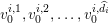 $v_{0}^{i,1},v_{0}^{i,2},\ldots ,v_{0}^{i,\widehat{d}_{i}}$
are linearly independent for all
 $i=1,2,\ldots ,d_{i}$
.
Note that we have not made any explicit assumptions on the integers
 $\widehat{d}_{i}$
and
 $\widehat{m}_{ij}$
in Theorem 2.15. If we assume that
 $\widehat{d}_{i}$
equals the geometric multiplicity of each
 $\unicode[STIX]{x1D706}_{i}$
, then if
 $(V,J)$
is a minimal pair the columns of each
 $V_{i}$
in Theorem 2.15 form a complete system of Jordan chains. In this case the algebraic multiplicities of the eigenvalues of
 $J$
coincide with the algebraic multiplicities of the corresponding eigenvalues of
 $F$
. This gives rise to the following definition.
Definition 2.16 (complete invariant pair).
An invariant pair
 $(V,M)$
of
 $F\in H(\unicode[STIX]{x1D6FA},\mathbb{C}^{n\times n})$
is called complete if it is minimal and the algebraic multiplicities of the eigenvalues of
 $M$
are the same as the algebraic multiplicities of the corresponding eigenvalues of
 $F$
.
Complete invariant pairs have been introduced by Kressner (Reference Kressner2009) under the name simple invariant pairs. We prefer to use the term complete as it better aligns with the terminology of a complete system of Jordan chains in Definition 2.3.
2.6 Nonlinear Rayleigh functionals
Nonlinear Rayleigh functionals are the generalization of Rayleigh quotients for matrices. Duffin (Reference Duffin1955) introduces them for symmetric overdamped quadratic eigenvalue problems. They are generalized to larger classes of Hermitian NEPs in Rogers (Reference Rogers1964), Hadeler (Reference Hadeler1967) and Voss (Reference Voss2009), and to general NEPs in Schreiber (Reference Schreiber2008) and Schwetlick and Schreiber (Reference Schwetlick and Schreiber2012).
Let
 $\unicode[STIX]{x1D706}$
be an eigenvalue of the matrix-valued function
 $F\in H(\unicode[STIX]{x1D6FA},\mathbb{C}^{n\times n})$
with corresponding right and left eigenvectors
 $v$
and
 $w$
. For some
 $\unicode[STIX]{x1D70C}>0$
and
 $\unicode[STIX]{x1D700}<\unicode[STIX]{x1D70B}/2$
, let
 $$\begin{eqnarray}\displaystyle \overline{\mathbb{D}}_{\unicode[STIX]{x1D706},\unicode[STIX]{x1D70C}} & = & \displaystyle \{z\in \mathbb{C}:~|z-\unicode[STIX]{x1D706}|\leq \unicode[STIX]{x1D70C}\},\nonumber\\ \displaystyle \overline{\mathbb{K}}_{\unicode[STIX]{x1D700}}(v) & = & \displaystyle \{x\in \mathbb{C}^{n}\setminus \{0\}:\angle (x,v)\leq \unicode[STIX]{x1D700}\}\nonumber\end{eqnarray}$$
be neighbourhoods of
 $\unicode[STIX]{x1D706}$
and
 $v$
, respectively. Here
 $\angle (x,v)$
denotes the angle between the nonzero vectors
 $x$
and
 $v$
, that is,
 $$\begin{eqnarray}\angle (x,v)=\cos ^{-1}\frac{|v^{\ast }x|}{\Vert x\Vert _{2}\Vert v\Vert _{2}}.\end{eqnarray}$$
A functional
 $$\begin{eqnarray}p:\overline{\mathbb{K}}_{\unicode[STIX]{x1D700}}(v)\times \overline{\mathbb{K}}_{\unicode[STIX]{x1D700}}(w)\ni (x,y)\mapsto p(x,y)\in \overline{\mathbb{D}}_{\unicode[STIX]{x1D706},\unicode[STIX]{x1D70C}}\end{eqnarray}$$
is a two-sided nonlinear Rayleigh functional if the following conditions hold:
 $$\begin{eqnarray}\displaystyle & & \displaystyle p(\unicode[STIX]{x1D6FC}x,\unicode[STIX]{x1D6FD}y)=p(x,y)\text{ for all nonzero }\unicode[STIX]{x1D6FC},\unicode[STIX]{x1D6FD}\in \mathbb{C},\end{eqnarray}$$
 $$\begin{eqnarray}\displaystyle & & \displaystyle y^{\ast }F(p(x,y))x=0,\end{eqnarray}$$
 $$\begin{eqnarray}\displaystyle & & \displaystyle y^{\ast }F^{\prime }(p(x,y))x\neq 0.\end{eqnarray}$$
The condition (2.20) restricts the functional to vectors close to eigenvectors corresponding to a simple eigenvalue.
The next result, which appears in Schwetlick and Schreiber (Reference Schwetlick and Schreiber2012, Theorem 5), concerns the local uniqueness of
 $p(x,y)$
and bounds the distance of
 $p(x,y)$
to the exact eigenvalue in terms of the angles between eigenvectors and approximations to eigenvectors.
Theorem 2.17. Let
 $\unicode[STIX]{x1D706}$
be a simple eigenvalue of
 $F\in H(\unicode[STIX]{x1D6FA},\mathbb{C}^{n\times n})$
with corresponding right and left eigenvectors
 $v$
and
 $w$
normalized to have unit
 $2$
-norms. Let
 $\unicode[STIX]{x1D70C}>0$
be such that
 $\overline{\mathbb{D}}_{\unicode[STIX]{x1D706},\unicode[STIX]{x1D70C}}\subset \unicode[STIX]{x1D6FA}$
. Then there exist constants
 $0<\unicode[STIX]{x1D70C}_{0}\leq \unicode[STIX]{x1D70C}$
,
 $0<\unicode[STIX]{x1D700}_{0}<\unicode[STIX]{x1D70B}/2$
such that for all
 $(x,y)\in \overline{\mathbb{K}}_{\unicode[STIX]{x1D700}_{0}}(v)\times \overline{\mathbb{K}}_{\unicode[STIX]{x1D700}_{0}}(w)$
there exists a unique
 $p(x,y)\in \overline{\mathbb{D}}_{\unicode[STIX]{x1D706},\unicode[STIX]{x1D70C}_{0}}$
satisfying
 $y^{\ast }F(p(x,y))x=0$
and
 $$\begin{eqnarray}|p(x,y)-\unicode[STIX]{x1D706}|\leq \frac{8}{3}\frac{\Vert F(\unicode[STIX]{x1D706})\Vert _{2}}{|y^{\ast }F^{\prime }(p(x,y))x|}\tan (\angle (x,v))\tan (\angle (y,w)).\end{eqnarray}$$
It then follows from Theorem 2.17 that
 $p(v,w)=\unicode[STIX]{x1D706}$
, that is,
 $p(v,w)$
is an eigenvalue of
 $F$
.
Example 2.18. Let
 $F$
be the matrix-valued function defined in (2.1), and let
 $\unicode[STIX]{x1D6FA}$
be the disc with centre
 $0$
and radius
 $3$
. If we let
 $x=[{x_{1}\atop x_{2}}]$
and
 $y=[{y_{1}\atop y_{2}}]$
then the condition (2.20) is equivalent to
 $p(x,y)\neq 0$
and
 $\overline{y}_{1}x_{1}\neq 0$
. Now if
 $\overline{y}_{1}x_{1}\neq 0$
, (2.19) can be rewritten as
 $$\begin{eqnarray}\text{e}^{\text{i}p(x,y)^{2}}=-\frac{\overline{y}_{1}x_{2}+\overline{y}_{2}x_{1}+\overline{y}_{2}x_{2}}{\overline{y}_{1}x_{1}}\end{eqnarray}$$
so that
 $$\begin{eqnarray}\text{i}p(x,y)^{2}=\log \biggl(-\displaystyle \frac{\overline{y}_{1}x_{2}+\overline{y}_{2}x_{1}+\overline{y}_{2}x_{2}}{\overline{y}_{1}x_{1}}\biggr)+2\unicode[STIX]{x1D70B}k\text{i},\quad k=0,\pm 1,\pm 2,\ldots\end{eqnarray}$$
for any complex logarithm function
 $\log$
. Hence the set of two-sided nonlinear Rayleigh functionals for
 $F$
is given by
 $$\begin{eqnarray}p(x,y)=\sqrt{-\text{i}\log (-\displaystyle \frac{\overline{y}_{1}x_{2}+\overline{y}_{2}x_{1}+\overline{y}_{2}x_{2}}{\overline{y}_{1}x_{1}}\biggr)+2\unicode[STIX]{x1D70B}k},\quad k=0,\pm 1,\pm 2,\ldots ,\end{eqnarray}$$
where for a complex number
 $z=\unicode[STIX]{x1D70C}\,\text{e}^{\text{i}\unicode[STIX]{x1D703}}$
,
 $\sqrt{z}=\pm \sqrt{\unicode[STIX]{x1D70C}}\,\text{e}^{\text{i}\unicode[STIX]{x1D703}/2}$
. Note that the functional
 $p(x,y)$
satisfies (2.18).
When
 $x=v$
and
 $y=w$
are right and left eigenvectors for
 $F$
with
 $v=w=[{1\atop -1}]$
, we recover the set of nonzero eigenvalues of
 $F$
,
 $$\begin{eqnarray}p(v,w)=\pm \sqrt{2\unicode[STIX]{x1D70B}k},\quad k=\pm 1,\pm 2,\ldots ,\end{eqnarray}$$
where we excluded
 $p(v,w)=0$
corresponding to
 $k=0$
since (2.20) implies that
 $p(v,w)\neq 0$
.
Schreiber (Reference Schreiber2008) shows that the nonlinear Rayleigh functional
 $p$
is stationary at the eigenvectors
 $(v,w)$
, that is,
 $$\begin{eqnarray}|p(v+\unicode[STIX]{x1D6E5}v,w+\unicode[STIX]{x1D6E5}w)-\unicode[STIX]{x1D706}|=O((\Vert \unicode[STIX]{x1D6E5}v\Vert _{2}+\Vert \unicode[STIX]{x1D6E5}w\Vert _{2})^{2}),\end{eqnarray}$$
where
 $\unicode[STIX]{x1D706}=p(v,w)$
. In other words, the first-order terms in a perturbation expansion of
 $p$
at the eigenvectors
 $(v,w)$
vanish identically.
2.7 Some perturbation results
It is often of interest, for example in sensitivity analysis and also in numerical computing, to give simple regions in which the eigenvalues of
 $F$
are located. Probably the most famous result for linear eigenvalue problems is Gershgorin’s theorem; see Horn and Johnson (Reference Horn and Johnson1991, Chapter 6). Bindel and Hood (Reference Bindel and Hood2013, Theorem 3.1) provide a generalization for NEPs.
Theorem 2.19 (Gershgorin’s theorem for NEPs).
Let
 $F(z)=D(z)+E(z)$
with
 $D,E\in H(\unicode[STIX]{x1D6FA},\mathbb{C}^{n\times n})$
and
 $D$
diagonal. Then, for any
 $0\leq \unicode[STIX]{x1D6FC}\leq 1$
,
 $$\begin{eqnarray}\unicode[STIX]{x1D6EC}(F)\subset \mathop{\bigcup }_{j=1}^{n}\mathbb{G}_{j}^{\unicode[STIX]{x1D6FC}},\end{eqnarray}$$
where
 $\mathbb{G}_{j}^{\unicode[STIX]{x1D6FC}}$
is the
 $j$
th generalized Gershgorin region
 $$\begin{eqnarray}\mathbb{G}_{j}^{\unicode[STIX]{x1D6FC}}=\{z\in \unicode[STIX]{x1D6FA}:|d_{jj}(z)|\leq r_{j}(z)^{\unicode[STIX]{x1D6FC}}c_{j}(z)^{1-\unicode[STIX]{x1D6FC}}\}\end{eqnarray}$$
and
 $r_{j}(z)$
,
 $c_{j}(z)$
are the
 $j$
th absolute row and column sums of
 $E$
, that is,
 $$\begin{eqnarray}r_{j}(z)=\mathop{\sum }_{k=1}^{n}|e_{jk}(z)|,\quad c_{j}(z)=\mathop{\sum }_{k=1}^{n}|e_{kj}(z)|.\end{eqnarray}$$
Moreover, if
 $\mathbb{U}$
is a bounded connected component of
 $\bigcup _{j=1}^{n}\mathbb{G}_{j}^{\unicode[STIX]{x1D6FC}}$
such that
 $\overline{\mathbb{U}}\subset \unicode[STIX]{x1D6FA}$
, then
 $\mathbb{U}$
contains the same number of eigenvalues of
 $F$
and
 $D$
. Furthermore, if
 $\mathbb{U}$
includes
 $p$
connected components of the Gershgorin regions, it must contain at least
 $p$
eigenvalues of
 $F$
.
Also of interest is the sensitivity of an eigenvalue
 $\unicode[STIX]{x1D706}$
of
 $F\in H(\unicode[STIX]{x1D6FA},\mathbb{C}^{n\times n})$
under small perturbations
 $\unicode[STIX]{x1D6E5}F\in H(\unicode[STIX]{x1D6FA},\mathbb{C}^{n\times n})$
. To address this point, we assume that
 $\unicode[STIX]{x1D706}$
is a nonzero simple eigenvalue with right eigenvector
 $v$
and left eigenvector
 $w$
. We consider
 $F$
expressed as in (2.15) with the perturbation
 $$\begin{eqnarray}\unicode[STIX]{x1D6E5}F(z)=f_{1}(z)\unicode[STIX]{x1D6E5}C_{1}+f_{2}(z)\unicode[STIX]{x1D6E5}C_{2}+\cdots +f_{\ell }(z)\unicode[STIX]{x1D6E5}C_{\ell }\in H(\unicode[STIX]{x1D6FA},\mathbb{C}^{n\times n}).\end{eqnarray}$$
To measure the sensitivity of
 $\unicode[STIX]{x1D706}$
, we can use the normwise condition number
 $$\begin{eqnarray}\displaystyle \unicode[STIX]{x1D705}(\unicode[STIX]{x1D706},F) & = & \displaystyle \limsup _{\unicode[STIX]{x1D700}\rightarrow 0}\biggl\{\frac{|\unicode[STIX]{x1D6E5}\unicode[STIX]{x1D706}|}{\unicode[STIX]{x1D700}|\unicode[STIX]{x1D706}|}:(F(\unicode[STIX]{x1D706}+\unicode[STIX]{x1D6E5}\unicode[STIX]{x1D706})+\unicode[STIX]{x1D6E5}F(\unicode[STIX]{x1D706}+\unicode[STIX]{x1D6E5}\unicode[STIX]{x1D706}))(v+\unicode[STIX]{x1D6E5}v)=0,\nonumber\\ \displaystyle & & \displaystyle \hspace{78.0pt}\vphantom{\frac{|\unicode[STIX]{x1D6E5}\unicode[STIX]{x1D706}|}{\unicode[STIX]{x1D700}|\unicode[STIX]{x1D706}|}}\Vert \unicode[STIX]{x1D6E5}C_{j}\Vert _{2}\leq \unicode[STIX]{x1D700}\unicode[STIX]{x1D6FC}_{j},~j=1,\ldots ,\ell \biggr\},\end{eqnarray}$$
where the
 $\unicode[STIX]{x1D6FC}_{j}$
are nonnegative parameters that allow freedom in how perturbations are measured – for example, in an absolute sense (
 $\unicode[STIX]{x1D6FC}_{j}=1$
) or in a relative sense (
 $\unicode[STIX]{x1D6FC}_{j}=\Vert C_{j}\Vert _{2}$
). By setting
 $\unicode[STIX]{x1D6FC}_{j}=0$
we can force
 $\unicode[STIX]{x1D6E5}C_{j}=0$
and thus keep
 $C_{j}$
unperturbed.
Theorem 2.20. The normwise condition number
 $\unicode[STIX]{x1D705}(\unicode[STIX]{x1D706},F)$
in (2.22) is
 $$\begin{eqnarray}\unicode[STIX]{x1D705}(\unicode[STIX]{x1D706},F)=\frac{(\mathop{\sum }_{j=1}^{\ell }\unicode[STIX]{x1D6FC}_{j}|f_{j}(\unicode[STIX]{x1D706})|)\Vert v\Vert _{2}\Vert w\Vert _{2}}{|\unicode[STIX]{x1D706}|\,|w^{\ast }F^{\prime }(\unicode[STIX]{x1D706})v|}.\end{eqnarray}$$
Proof. By expanding the first constraint in (2.22) and keeping only the first-order terms, we get
 $$\begin{eqnarray}\unicode[STIX]{x1D6E5}\unicode[STIX]{x1D706}F^{\prime }(\unicode[STIX]{x1D706})v+F(\unicode[STIX]{x1D706})\unicode[STIX]{x1D6E5}v+\unicode[STIX]{x1D6E5}F(\unicode[STIX]{x1D706})v=O(\unicode[STIX]{x1D700}^{2}).\end{eqnarray}$$
Premultiplying by
 $w^{\ast }$
leads to
 $$\begin{eqnarray}\unicode[STIX]{x1D6E5}\unicode[STIX]{x1D706}w^{\ast }F^{\prime }(\unicode[STIX]{x1D706})v+w^{\ast }\unicode[STIX]{x1D6E5}F(\unicode[STIX]{x1D706})v=O(\unicode[STIX]{x1D700}^{2}).\end{eqnarray}$$
Since
 $\unicode[STIX]{x1D706}$
is a simple eigenvalue, we have from (2.5) that
 $w^{\ast }F^{\prime }(\unicode[STIX]{x1D706})v\neq 0$
. Thus
 $$\begin{eqnarray}\unicode[STIX]{x1D6E5}\unicode[STIX]{x1D706}=-\frac{w^{\ast }\unicode[STIX]{x1D6E5}F(\unicode[STIX]{x1D706})v}{w^{\ast }F^{\prime }(\unicode[STIX]{x1D706})v}+O(\unicode[STIX]{x1D700}^{2})\end{eqnarray}$$
and so
 $$\begin{eqnarray}\frac{|\unicode[STIX]{x1D6E5}\unicode[STIX]{x1D706}|}{\unicode[STIX]{x1D700}|\unicode[STIX]{x1D706}|}\leq \frac{(\mathop{\sum }_{j=1}^{\ell }\unicode[STIX]{x1D6FC}_{j}|f_{j}(\unicode[STIX]{x1D706})|)\Vert w\Vert _{2}\Vert v\Vert _{2}}{|\unicode[STIX]{x1D706}|\,|w^{\ast }F^{\prime }(\unicode[STIX]{x1D706})v|}+O(\unicode[STIX]{x1D700}).\end{eqnarray}$$
Hence the expression on the right-hand side of
 $\unicode[STIX]{x1D705}(\unicode[STIX]{x1D706},F)$
in the theorem is an upper bound for the condition number. To show that this bound can be attained we consider the matrix
 $H=wv^{\ast }/(\Vert w\Vert _{2}\Vert v\Vert _{2})$
, for which
 $$\begin{eqnarray}\Vert H\Vert _{2}=1,\quad w^{\ast }Hv=\Vert v\Vert _{2}\Vert w\Vert _{2}.\end{eqnarray}$$
Let
 $$\begin{eqnarray}\unicode[STIX]{x1D6E5}C_{j}=\unicode[STIX]{x1D700}\unicode[STIX]{x1D6FC}_{j}\frac{\overline{f_{j}(\unicode[STIX]{x1D706})}}{|f_{j}(\unicode[STIX]{x1D706})|}H,\quad j=1,\ldots ,\ell .\end{eqnarray}$$
Then all the norm inequalities in (2.22) are satisfied as equalities and
 $$\begin{eqnarray}|w^{\ast }\unicode[STIX]{x1D6E5}F(\unicode[STIX]{x1D706})v|=\unicode[STIX]{x1D700}\,\biggl(\mathop{\sum }_{j=1}^{\ell }\unicode[STIX]{x1D6FC}_{j}|f_{j}(\unicode[STIX]{x1D706})|\biggr)\Vert w\Vert _{2}\Vert v\Vert _{2}.\end{eqnarray}$$
Dividing by
 $\unicode[STIX]{x1D700}|\unicode[STIX]{x1D706}|\,|w^{\ast }F^{\prime }(\unicode[STIX]{x1D706})v|$
and taking the limit as
 $\unicode[STIX]{x1D700}\rightarrow 0$
gives the desired equality.
Pseudospectra are another established tool for gaining insight into the sensitivity of the eigenvalues of a matrix to perturbations; see Trefethen and Embree (Reference Trefethen and Embree2005) and the references therein. The
 $\unicode[STIX]{x1D700}$
-pseudospectrum of
 $F\in H(\unicode[STIX]{x1D6FA},\mathbb{C}^{n\times n})$
is the set
 $$\begin{eqnarray}\unicode[STIX]{x1D6EC}_{\unicode[STIX]{x1D700}}(F)=\mathop{\bigcup }_{\substack{ \unicode[STIX]{x1D6E5}F\in H(\unicode[STIX]{x1D6FA},\mathbb{C}^{n\times n}) \\ \Vert \unicode[STIX]{x1D6E5}F\Vert <\unicode[STIX]{x1D700}}}\unicode[STIX]{x1D6EC}(F+\unicode[STIX]{x1D6E5}F),\end{eqnarray}$$
where, for example,
 $$\begin{eqnarray}\Vert \unicode[STIX]{x1D6E5}F\Vert =\Vert \unicode[STIX]{x1D6E5}F\Vert _{\unicode[STIX]{x1D6FA}}:=\sup _{z\in \unicode[STIX]{x1D6FA}}\Vert \unicode[STIX]{x1D6E5}F(z)\Vert _{2}.\end{eqnarray}$$
If
 $F$
is expressed as in (2.15), then we can consider perturbations
 $\unicode[STIX]{x1D6E5}F$
of the form (2.21) and measure them using
 $$\begin{eqnarray}\Vert \unicode[STIX]{x1D6E5}F\Vert =\Vert \unicode[STIX]{x1D6E5}F\Vert _{\max }:=\max _{1\leq j\leq \ell }\Vert \unicode[STIX]{x1D6E5}F_{j}\Vert _{2}/\unicode[STIX]{x1D6FC}_{j},\end{eqnarray}$$
where the
 $\unicode[STIX]{x1D6FC}_{j}$
are nonnegative parameters defined as for (2.22). Other measures of the perturbations can be used too; see for example Tisseur and Higham (Reference Tisseur and Higham2001), Higham and Tisseur (Reference Higham and Tisseur2002) and Michiels, Green, Wagenknecht and Niculescu (Reference Michiels, Green, Wagenknecht and Niculescu2006).
The following characterizations of
 $\unicode[STIX]{x1D6EC}_{\unicode[STIX]{x1D700}}(F)$
(see Bindel and Hood Reference Bindel and Hood2013, Proposition 4.1, and Michiels et al.
Reference Michiels, Green, Wagenknecht and Niculescu2006, Theorem 1) provide an easy way to check whether a point
 $z\in \unicode[STIX]{x1D6FA}$
is in the
 $\unicode[STIX]{x1D700}$
-pseudospectrum of
 $F$
or not.
Theorem 2.21. Let
 $F\in H(\unicode[STIX]{x1D6FA},\mathbb{C}^{n\times n})$
. Then, for
 $\unicode[STIX]{x1D6EC}_{\unicode[STIX]{x1D700}}(F)$
defined by (2.23),
 $$\begin{eqnarray}\unicode[STIX]{x1D6EC}_{\unicode[STIX]{x1D700}}(F)=\{z\in \unicode[STIX]{x1D6FA}:\Vert F(z)^{-1}\Vert _{2}>(\unicode[STIX]{x1D700}f(z))^{-1}\},\end{eqnarray}$$
where
 $f(z)=1$
when the perturbations are measured using (2.24), and
 $f(z)=\sum _{j=1}^{\ell }\unicode[STIX]{x1D6FC}_{j}|f_{j}(z)|$
when the perturbations are measured using (2.25).
The
 $\unicode[STIX]{x1D700}$
-pseudospectrum is connected to the backward error of an approximate eigenvalue
 $\widetilde{\unicode[STIX]{x1D706}}$
of
 $F$
defined by
 $$\begin{eqnarray}\unicode[STIX]{x1D702}_{F}(\widetilde{\unicode[STIX]{x1D706}})=\min _{{v\in \mathbb{C}^{n}\atop v\neq 0}}\unicode[STIX]{x1D702}_{F}(\widetilde{\unicode[STIX]{x1D706}},v),\end{eqnarray}$$
where
 $$\begin{eqnarray}\unicode[STIX]{x1D702}_{F}(\widetilde{\unicode[STIX]{x1D706}},v)=\min \{\unicode[STIX]{x1D700}:(F(\widetilde{\unicode[STIX]{x1D706}})+\unicode[STIX]{x1D6E5}F(\widetilde{\unicode[STIX]{x1D706}}))v=0,~\Vert \unicode[STIX]{x1D6E5}F\Vert \leq \unicode[STIX]{x1D700}\}\end{eqnarray}$$
with perturbations measured using, for example, (2.24) or (2.25). Then, by comparing the definitions (2.23) and (2.26), we have that
 $$\begin{eqnarray}\unicode[STIX]{x1D6EC}_{\unicode[STIX]{x1D700}}(F)=\{z\in \unicode[STIX]{x1D6FA}:\unicode[STIX]{x1D702}_{F}(z)<\unicode[STIX]{x1D700}\}.\end{eqnarray}$$
For an approximate eigenpair
 $(\widetilde{\unicode[STIX]{x1D706}},\widetilde{v})$
of
 $F$
and for perturbations measured using (2.25), a straightforward generalization of Tisseur (Reference Tisseur2000, Theorem 1 and Lemma 3) leads to explicit expressions for
 $\unicode[STIX]{x1D702}_{F}(\widetilde{\unicode[STIX]{x1D706}},\widetilde{v})$
and
 $\unicode[STIX]{x1D702}_{F}(\widetilde{\unicode[STIX]{x1D706}})$
,
 $$\begin{eqnarray}\unicode[STIX]{x1D702}_{F}(\widetilde{\unicode[STIX]{x1D706}},\widetilde{v})=\frac{\Vert F(\widetilde{\unicode[STIX]{x1D706}})\widetilde{v}\Vert _{2}}{f(\widetilde{\unicode[STIX]{x1D706}})\,\Vert \widetilde{v}\Vert _{2}}\quad \text{and}\quad \unicode[STIX]{x1D702}_{F}(\widetilde{\unicode[STIX]{x1D706}})=\frac{1}{f(\widetilde{\unicode[STIX]{x1D706}})\,\Vert F(\widetilde{\unicode[STIX]{x1D706}})^{-1}\Vert _{2}},\end{eqnarray}$$
where
 $f(\widetilde{\unicode[STIX]{x1D706}})=\sum _{j=1}^{\ell }\unicode[STIX]{x1D6FC}_{j}|f_{j}(\widetilde{\unicode[STIX]{x1D706}})|$
.
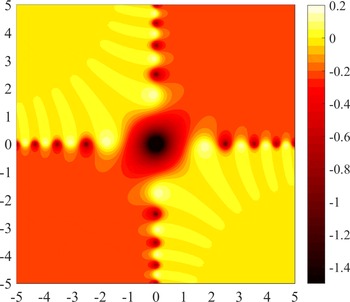
Spectral portrait of the matrix-valued function
 $F$
defined in (2.1). The bar shows the mapping of colours to
 $\log _{10}$
of the resolvent norm, that is, the mapping
 $z\mapsto \log _{10}\Vert F(z)^{-1}\Vert _{2}$
.

Example 2.23. Let us consider once more the function
 $F$
from (2.1), now rewritten in the form
 $$\begin{eqnarray}F(z)=\text{e}^{\text{i}z^{2}}\left[\begin{array}{@{}cc@{}}1 & 0\\ 0 & 0\end{array}\right]+\left[\begin{array}{@{}cc@{}}0 & 1\\ 1 & 1\end{array}\right]=:f_{1}(z)C_{1}+f_{2}(z)C_{2}.\end{eqnarray}$$
An easy computation shows that the nonzero eigenvalues of
 $F$
,
 $\unicode[STIX]{x1D706}_{k}=\pm \sqrt{2\unicode[STIX]{x1D70B}k}$
,
 $k=\pm 1,\pm 2,\ldots ,$
have small condition numbers
 $$\begin{eqnarray}\unicode[STIX]{x1D705}(\unicode[STIX]{x1D706}_{k},F)=\frac{1+\sqrt{1+(3+5^{1/2})/2}}{2\unicode[STIX]{x1D70B}|k|},\end{eqnarray}$$
and these condition numbers get smaller as
 $k$
increases in modulus. This is confirmed by the spectral portrait in Figure 2.22, which shows that nonzero eigenvalues of
 $F$
move only slightly even under very large perturbations of
 $F$
. The zero eigenvalue is defective and more sensitive to perturbations.
The largest possible real part of points in the
 $\unicode[STIX]{x1D700}$
-pseudospectrum of
 $F$
is called the
 $\unicode[STIX]{x1D700}$
-pseudospectral abscissa of
 $F$
, that is,
 $$\begin{eqnarray}\unicode[STIX]{x1D6FC}_{\unicode[STIX]{x1D700}}(F)=\max \{\Re (z):z\in \unicode[STIX]{x1D6EC}_{\unicode[STIX]{x1D700}}(F)\}.\end{eqnarray}$$
This quantity is of particular interest for NEPs associated with systems of differential equations such as the DDE (1.1), since perturbations of size
 $\unicode[STIX]{x1D700}$
may cause the system to become unstable whenever
 $\unicode[STIX]{x1D6FC}_{\unicode[STIX]{x1D700}}(F)\geq 0$
. The distance to instability of a stable system associated with
 $F$
can then be defined as
 $$\begin{eqnarray}\unicode[STIX]{x1D6FF}(F)=\inf \{\unicode[STIX]{x1D700}:\unicode[STIX]{x1D6FC}_{\unicode[STIX]{x1D700}}(F)\geq 0\}.\end{eqnarray}$$
Algorithms to compute
 $\unicode[STIX]{x1D6FC}_{\unicode[STIX]{x1D700}}(F)$
can be found in Michiels and Guglielmi (Reference Michiels and Guglielmi2012) and Verhees et al. (Reference Verhees, Van Beeumen, Meerbergen, Guglielmi and Michiels2014).
3 Hermitian NEPs
A matrix-valued function
 $F(z)$
is said to be Hermitian if
 $F(\bar{z})=F(z)^{\ast }$
for all
 $z\in \mathbb{C}$
. It is easily seen that the eigenvalues of a Hermitian
 $F$
are either real or they come in pairs
 $(\unicode[STIX]{x1D706},\bar{\unicode[STIX]{x1D706}})$
. If
 $v$
and
 $w$
are right and left eigenvectors of
 $F$
for the eigenvalue
 $\unicode[STIX]{x1D706}\in \mathbb{C}$
, then
 $w$
and
 $v$
are right and left eigenvectors of
 $F$
for the eigenvalue
 $\bar{\unicode[STIX]{x1D706}}$
, whereas if
 $\unicode[STIX]{x1D706}$
is a real eigenvalue of
 $F$
for the right eigenvector
 $v$
, then
 $v$
is also a left eigenvector for the eigenvalue
 $\unicode[STIX]{x1D706}$
.
As for Hermitian linear eigenvalue problems, variational principles for real eigenvalues of Hermitian NEPs exist, as we now discuss. For this we assume that the assumptions (A1)–(A3) below hold.
-
(A1) The matrix-valued function
$F:\mathbb{R}\supseteq \mathbb{I}\rightarrow \mathbb{C}^{n\times n}$
is Hermitian and continuously differentiable on the open real interval
$\mathbb{I}$
.


-
(A2) For every
$x\in \mathbb{C}^{n}\setminus \{0\}$
, the real nonlinear equation (3.1)has at most one real solution
$$\begin{eqnarray}x^{\ast }F(p(x))x=0\end{eqnarray}$$
$p(x)\in \mathbb{I}$
.


Note that (3.1) defines implicitly the one-sided generalized Rayleigh functional
 $p$
on some open subset
 $\mathbb{K}(p)\subseteq \mathbb{C}^{n}\setminus \{0\}$
. When the Rayleigh functional
 $p$
is defined on the whole space
 $\mathbb{C}^{n}\setminus \{0\}$
, the NEP
 $F(\unicode[STIX]{x1D706})v=0$
is called overdamped.
-
(A3) For every
$x\in \mathbb{K}(p)$
and any
$z\in \mathbb{I}$
such that
$z\neq p(x)$
, (3.2)that is,
$$\begin{eqnarray}(z-p(x))(x^{\ast }F(z)x)>0,\end{eqnarray}$$
$x^{\ast }F(z)x$
is increasing at
$z=p(x)$
.


When
 $F$
is overdamped, assumption (A3) holds if
 $x^{\ast }F^{\prime }(p(x))x>0$
for all
 $x\in \mathbb{C}^{n}\setminus \{0\}$
. Moreover, if
 $F$
is overdamped and twice continuously differentiable, and
 $x^{\ast }F^{\prime \prime }(p(x))x\neq 0$
for all
 $x\in \mathbb{C}^{n}\setminus \{0\}$
, then (3.2) is equivalent to
 $x^{\ast }F^{\prime }(p(x))x>0$
for all
 $x\in \mathbb{C}^{n}\setminus \{0\}$
(Szyld and Xue Reference Szyld and Xue2016, Proposition 2.4).
Let
 $\unicode[STIX]{x1D706}\in \mathbb{I}$
be an eigenvalue of
 $F$
; then
 $\unicode[STIX]{x1D706}$
is called a
 $k$
th eigenvalue of
 $F$
if
 $\unicode[STIX]{x1D707}=0$
is the
 $k$
th largest eigenvalue of the Hermitian matrix
 $F(\unicode[STIX]{x1D706})$
. The next result, which can be found in Hadeler (Reference Hadeler1968), Voss and Werner (Reference Voss and Werner1982) and Voss (Reference Voss2009), provides a minmax characterization and a maxmin characterization of the real eigenvalues of
 $F$
.
Theorem 3.1 (nonlinear variational principle).
Assume the matrix-valued function
 $F$
satisfies (A1)–(A3). Then
 $F$
has at most
 $n$
eigenvalues in
 $\mathbb{I}$
. Moreover, if
 $\unicode[STIX]{x1D706}_{k}$
is a
 $k$
th eigenvalue of
 $F$
, then
 $$\begin{eqnarray}\displaystyle \unicode[STIX]{x1D706}_{k} & = & \displaystyle \min _{\substack{ V\in \mathbb{S}_{k} \\ V\cap \mathbb{K}(p)\neq \emptyset }}\,\max _{\substack{ x\in V\cap \mathbb{K}(p) \\ x\neq 0}}\,p(x)\in \mathbb{I},\end{eqnarray}$$
 $$\begin{eqnarray}\displaystyle \unicode[STIX]{x1D706}_{k} & = & \displaystyle \max _{\substack{ V\in \mathbb{S}_{k-1} \\ V^{\bot }\cap \mathbb{K}(p)\neq \emptyset }}\,\min _{\substack{ x\in V^{\bot }\cap \mathbb{K}(p) \\ x\neq 0}}\,p(x)\in \mathbb{I},\end{eqnarray}$$
where
 $\mathbb{S}_{j}$
denotes the set of all subspaces of
 $\mathbb{C}^{n}$
of dimension
 $j$
.
The characterization of the eigenvalues in (3.3) is a generalization of the minmax principle of Poincaré (Reference Poincaré1890) for linear eigenvalue problems and that in (3.4) is a generalization of the maxmin characterization of Courant (Reference Courant1920), Fischer (Reference Fischer1905) and Weyl (Reference Weyl1912).
When
 $F$
satisfies (A1)–(A3) and is overdamped, then there exist exactly
 $n$
eigenvalues
 $\unicode[STIX]{x1D706}_{1},\unicode[STIX]{x1D706}_{2},\ldots ,\unicode[STIX]{x1D706}_{n}$
of
 $F$
in
 $\mathbb{I}$
, and it follows from Theorem 3.1 that
 $\unicode[STIX]{x1D706}_{1}\leq \unicode[STIX]{x1D706}_{2}\leq \cdots \leq \unicode[STIX]{x1D706}_{n}$
, thereby offering an ordering of the real eigenvalues of
 $F$
in
 $\mathbb{I}$
. The variational principle can be used to derive an interesting property of eigenvalue approximations obtained by projecting
 $F$
onto low-dimensional spaces; see Szyld and Xue (Reference Szyld and Xue2016, Theorem 2.7).
Theorem 3.2 (nonlinear Cauchy interlacing theorem).
Assume that
 $F$
satisfies (A1)–(A3) and is overdamped, with eigenvalues
 $\unicode[STIX]{x1D706}_{1}\leq \unicode[STIX]{x1D706}_{2}\leq \cdots \leq \unicode[STIX]{x1D706}_{n}\in \mathbb{I}$
. Let
 $U\in \mathbb{C}^{n\times k}$
be of full column rank. Then the projected matrix-valued function
 $U^{\ast }F(z)U$
has exactly
 $k$
eigenvalues satisfying the nonlinear variational principle, and if
 $\unicode[STIX]{x1D707}_{j}$
is the
 $j$
th eigenvalue of
 $U^{\ast }F(z)U$
then
 $\unicode[STIX]{x1D706}_{j}\leq \unicode[STIX]{x1D707}_{j}\leq \unicode[STIX]{x1D706}_{n-k+j}$
.
The nonlinear Cauchy interlacing theorem and the variational principle in Theorem 3.1 allow the development of special algorithms for Hermitian NEPs satisfying the assumptions (A1)–(A3) in Section 4.6.
Example 3.3. Let us consider the loaded_string problem with
 $F$
defined in (1.3). The associated quadratic matrix polynomial
 $$\begin{eqnarray}Q(z)=-(z-1)F(z)=z^{2}C_{2}-z(C_{1}+C_{2}+C_{3})+C_{1}\end{eqnarray}$$
is hyperbolic, since its leading matrix coefficient
 $C_{2}$
is positive definite and the scalar equation
 $x^{\ast }Q(z)x=0$
has two distinct real roots (Al-Ammari and Tisseur Reference Al-Ammari and Tisseur2012, Theorem 3.4). As a result,
 $Q$
has only real eigenvalues. But clearly, if
 $\unicode[STIX]{x1D706}$
is an eigenvalue of
 $F$
, then it is an eigenvalue of
 $Q$
. Hence
 $F$
has only real eigenvalues. For
 $n=100$
the first nine eigenvalues of
 $F$
greater than
 $1$
are given to 10 digits by

(see Solov’ëv Reference Solov’ëv2006), and there is also an eigenvalue smaller than
 $1$
,

Compared to
 $F$
,
 $Q$
has
 $n-1$
extra eigenvalues at
 $z=1$
.
It is easy to check that property (A1) holds on the interval
 $\mathbb{I}=(1,+\infty )$
. If we let
 $$\begin{eqnarray}a(x)=x^{\ast }C_{2}x,\quad b(x)=-x^{\ast }(C_{1}+C_{2}+C_{3})x,\quad c(x)=x^{\ast }C_{1}x,\end{eqnarray}$$
then
 $$\begin{eqnarray}p(x)=\frac{-b(x)+\sqrt{b^{2}(x)-4a(x)c(x)}}{2a(x)}>1\end{eqnarray}$$
is well defined for every
 $x\in \mathbb{C}^{n}\setminus \{0\}$
since
 $a(x)>0$
, and it is the only root of
 $x^{\ast }F(p(x))x=0$
in
 $\mathbb{I}$
. Hence property (A2) holds and
 $F$
is overdamped on
 $\mathbb{I}$
. Now,
 $$\begin{eqnarray}x^{\ast }F^{\prime }(z)x=-x^{\ast }C_{2}x-\frac{1}{(z-1)^{2}}x^{\ast }C_{3}x<0\end{eqnarray}$$
for all
 $x\in \mathbb{C}^{n}\setminus \{0\}$
, so that property (A3) holds for
 $-F(z)$
. As a result, the eigenvalues of
 $F$
in
 $\mathbb{I}$
satisfy the nonlinear variational principle in Theorem 3.1.
4 Solvers based on Newton’s method
Newton’s method is a natural approach to compute eigenvalues or eigenpairs of NEPs efficiently and accurately provided that good initial guesses are available. The choice of an initial guess is typically the only crucial parameter of a Newton-type method, which is a great advantage over other NEP solution approaches. As a result, many algorithmic variants have been developed and applied over the years, including the Newton-QR iteration of Kublanovskaya (Reference Kublanovskaya1970) and its variant in Garrett, Bai and Li (Reference Garrett, Bai and Li2016), the Newton-trace iteration of Lancaster (Reference Lancaster1966), nonlinear inverse iteration (Unger Reference Unger1950), residual inverse iteration (Neumaier Reference Neumaier1985), Rayleigh functional iterations (Lancaster Reference Lancaster1961, Schreiber Reference Schreiber2008), the block Newton method of Kressner (Reference Kressner2009), and for large sparse NEPs, Jacobi–Davidson-type methods (Betcke and Voss Reference Betcke and Voss2004, Sleijpen, Booten, Fokkema and van der Vorst Reference Sleijpen, Booten, Fokkema and van der Vorst1996).
Generally speaking, there are two broad ways the NEP
 $F(\unicode[STIX]{x1D706})v=0$
can be tackled by a Newton-type method. First, one can apply Newton’s method to a scalar equation
 $f(z)=0$
whose roots correspond to the wanted eigenvalues of
 $F$
, or second, Newton’s method can be applied directly to the vector problem
 $F(\unicode[STIX]{x1D706})v=0$
together with some normalization condition on
 $v$
. We discuss both approaches.
4.1 Newton’s method for scalar functions
For a given initial guess
 $\unicode[STIX]{x1D706}^{(0)}$
, Newton’s method for finding the roots of a scalar equation
 $f(z)=0$
is given by
 $$\begin{eqnarray}\unicode[STIX]{x1D706}^{(k+1)}=\unicode[STIX]{x1D706}^{(k)}-\frac{f(\unicode[STIX]{x1D706}^{(k)})}{f^{\prime }(\unicode[STIX]{x1D706}^{(k)})},\quad k=0,1,\ldots .\end{eqnarray}$$
This iteration has local quadratic convergence to simple roots (Wilkinson Reference Wilkinson1965, Section 7.25). In order to apply it to the solution of an NEP
 $F(\unicode[STIX]{x1D706})v=0$
, we only need a scalar function
 $f$
whose roots are the eigenvalues of
 $F$
, and its derivative
 $f^{\prime }$
. Different methods result from different choices of
 $f$
.
Probably the most obvious choice is
 $$\begin{eqnarray}f(z)=\det F(z).\end{eqnarray}$$
The trace theorem (e.g. Lancaster Reference Lancaster1966, Theorem 5.1), states that if the entries of
 $F(z)$
are differentiable functions of
 $z$
, then for any
 $z\in \mathbb{C}$
for which
 $f(z)=\det F(z)\neq 0$
we have
 $$\begin{eqnarray}f^{\prime }(z)=\det F(z)\operatorname{trace}(F^{-1}(z)F^{\prime }(z)),\end{eqnarray}$$
and so the Newton iteration (4.1) can be rewritten as
 $$\begin{eqnarray}\unicode[STIX]{x1D706}^{(k+1)}=\unicode[STIX]{x1D706}^{(k)}-\frac{1}{\operatorname{trace}(F^{-1}(\unicode[STIX]{x1D706}^{(k)})F^{\prime }(\unicode[STIX]{x1D706}^{(k)}))},\quad k=0,1,\ldots .\end{eqnarray}$$
We refer to (4.3) as the Newton-trace iteration (Lancaster Reference Lancaster1966, Section 5.5); see also Khazanov and Kublanovskaya (Reference Khazanov and Kublanovskaya1988). Note that we only need the diagonal entries of
 $F^{-1}(\unicode[STIX]{x1D706}^{(k)})F^{\prime }(\unicode[STIX]{x1D706}^{(k)})$
. Nevertheless, with a straightforward implementation each iteration requires the factorization of an
 $n\times n$
matrix
 $F(\unicode[STIX]{x1D706}^{(k)})$
and
 $2n$
triangular solves, making it a rather expensive method. A basic MATLAB implementation of the Newton-trace iteration (4.2) is provided in Figure 4.1, where we use a simple stopping criterion based on the relative residual
 $|f(\unicode[STIX]{x1D706}^{(k)})|/\Vert F(\unicode[STIX]{x1D706}^{(k)})\Vert _{F}$
.


Kublanovskaya (Reference Kublanovskaya1970) proposes applying Newton’s method to
 $$\begin{eqnarray}f(z)=r_{nn}(z),\end{eqnarray}$$
where
 $r_{nn}(z)$
is the bottom-right entry of the
 $R$
factor in a rank-revealing QR decomposition of
 $F(z)$
,
 $$\begin{eqnarray}F(z)\unicode[STIX]{x1D6F1}(z)=Q(z)R(z),\end{eqnarray}$$
with
 $\unicode[STIX]{x1D6F1}(z)$
being a permutation matrix which ensures that
 $r_{nn}(z)$
becomes zero before any other diagonal entry does; see also Kublanovskaja (Reference Kublanovskaja1969). Since
 $r_{nn}(z)=0$
is equivalent to
 $\det F(z)=\det R(z)=0$
, we know that the roots of
 $f(z)$
are exactly the roots of
 $\det F(z)=0$
.
The permutation
 $\unicode[STIX]{x1D6F1}(z)$
in (4.4) is not a continuous function of
 $z$
, but in a small neighbourhood of an approximate eigenvalue
 $\unicode[STIX]{x1D706}^{(k)}$
of
 $F$
the permutation can be kept constant. So if we let
 $$\begin{eqnarray}F(\unicode[STIX]{x1D706}^{(k)})\unicode[STIX]{x1D6F1}=Q_{k}R_{k}=Q_{k}\left[\begin{array}{@{}cc@{}}R_{11}^{(k)} & r_{12}^{(k)}\\ 0 & r_{nn}^{(k)}\end{array}\right]\!,\end{eqnarray}$$
then in a small neighbourhood of
 $\unicode[STIX]{x1D706}_{k}^{(k)}$
we can use
 $$\begin{eqnarray}F(z)\unicode[STIX]{x1D6F1}=Q(z)R(z)=Q(z)\left[\begin{array}{@{}cc@{}}R_{11}(z) & r_{12}(z)\\ 0 & r_{nn}(z)\end{array}\right]\end{eqnarray}$$
with
 $Q(\unicode[STIX]{x1D706}^{(k)})=Q_{k}$
and
 $R(\unicode[STIX]{x1D706}^{(k)})=R_{k}$
. Garrett et al. (Reference Garrett, Bai and Li2016) show that
 $$\begin{eqnarray}r_{nn}(z)=r_{nn}^{(k)}+e_{n}^{T}Q_{k}^{\ast }F^{\prime }(\unicode[STIX]{x1D706}^{(k)})\unicode[STIX]{x1D6F1}\left[\begin{array}{@{}c@{}}-p\\ 1\end{array}\right](z-\unicode[STIX]{x1D706}^{(k)})+O(|z-\unicode[STIX]{x1D706}^{(k)}|^{2}),\end{eqnarray}$$
where
 $e_{n}=[0,\ldots ,0,1]^{T}$
and
 $p$
solves
 $R_{11}^{(k)}p=r_{12}^{(k)}$
, and therefore
 $$\begin{eqnarray}r_{nn}^{\prime }(\unicode[STIX]{x1D706}^{(k)})=e_{n}^{T}Q_{k}^{\ast }F^{\prime }(\unicode[STIX]{x1D706}^{(k)})\unicode[STIX]{x1D6F1}\left[\begin{array}{@{}c@{}}-p\\ 1\end{array}\right]\!.\end{eqnarray}$$
This leads to the Newton-QR iteration for a root of
 $r_{nn}(z)$
,
 $$\begin{eqnarray}\unicode[STIX]{x1D706}^{(k+1)}=\unicode[STIX]{x1D706}^{(k)}-\frac{r_{nn}(\unicode[STIX]{x1D706}^{(k)})}{r_{nn}^{\prime }(\unicode[STIX]{x1D706}^{(k)})}=\unicode[STIX]{x1D706}^{(k)}-\frac{r_{nn}^{(k)}}{e_{n}^{T}Q_{k}^{\ast }F^{\prime }(\unicode[STIX]{x1D706}^{(k)})\unicode[STIX]{x1D6F1}[{-p\atop 1}]}.\end{eqnarray}$$
At convergence, we can take
 $$\begin{eqnarray}v=\unicode[STIX]{x1D6F1}\left[\begin{array}{@{}c@{}}-p\\ 1\end{array}\right]\!,\quad w=Q_{k}e_{n}\end{eqnarray}$$
as approximations for the right and left eigenvectors of the converged approximate eigenvalue, respectively.
Basic MATLAB implementation of the Newton-QR iteration for problem (2.1). The NEP parameters
 $F$
and
 $F^{\prime }$
are specified in lines 2–3 and the method’s parameters in line 4. Upon convergence, lambda is the eigenvalue and nbr_iter the number of iterations.

A basic MATLAB implementation of the Newton-QR iteration (4.6) is given in Figure 4.2. It requires the repeated computation of a rank-revealing QR factorization of
 $F(\unicode[STIX]{x1D706}^{(k)})$
and hence is only feasible for problems of moderate size (unless
 $F$
has some structure that can be exploited; see Section 4.5). However, the iteration (4.6) can be useful in the context of iterative refinement. Yang (Reference Yang1983) and Wobst (Reference Wobst1987) consider an approach similar to that of Kublanovskaya by using an LU factorization with column pivoting in place of a rank-revealing QR factorization.
To avoid working with nearly singular matrices
 $F(\unicode[STIX]{x1D706}^{(k)})$
, Andrew, Chu and Lancaster (Reference Andrew, Chu and Lancaster1995) propose using in place of
 $F(z)$
the bordered matrix
 $$\begin{eqnarray}G(z)=\left[\begin{array}{@{}cc@{}}F(z) & b\\ c^{T} & 0\end{array}\right]\!,\end{eqnarray}$$
where
 $b,c\in \mathbb{C}^{n}$
are such that the matrix
 $G(\unicode[STIX]{x1D706})$
is nonsingular and well-conditioned at a simple eigenvalue
 $\unicode[STIX]{x1D706}$
. Now if
 $c^{T}v\neq 0$
and
 $w^{T}b\neq 0$
, where
 $v$
and
 $w$
are the right and left eigenvectors of
 $F$
associated with the eigenvalue
 $\unicode[STIX]{x1D706}$
, then
 $G(\unicode[STIX]{x1D706})$
is nonsingular (Andrew, Chu and Lancaster Reference Andrew, Chu and Lancaster1993, Theorem 10.1). For a vector
 $x$
such that
 $c^{T}x=1$
, the authors introduce the linear system
 $$\begin{eqnarray}\left[\begin{array}{@{}cc@{}}F(z) & b\\ c^{T} & 0\end{array}\right]\left[\begin{array}{@{}c@{}}x\\ f\end{array}\right]=\left[\begin{array}{@{}c@{}}0\\ 1\end{array}\right]\!.\end{eqnarray}$$
For
 $z$
near
 $\unicode[STIX]{x1D706}$
, the matrix
 $G(z)$
is nonsingular and hence
 $x=x(z)$
and
 $f=f(z)$
are smooth functions of
 $z$
. By Cramer’s rule we have
 $$\begin{eqnarray}f(z)=\frac{\det F(z)}{\det G(z)},\end{eqnarray}$$
and therefore
 $f(z)=0$
if and only if
 $\det F(z)=0$
. Differentiating (4.8) with respect to
 $z$
leads to
 $$\begin{eqnarray}\left[\begin{array}{@{}cc@{}}F(z) & b\\ c^{T} & 0\end{array}\right]\left[\begin{array}{@{}c@{}}x^{\prime }(z)\\ f^{\prime }(z)\end{array}\right]=-\left[\begin{array}{@{}c@{}}F^{\prime }(z)x(z)\\ 0\end{array}\right]\!.\end{eqnarray}$$
The BDS method of Andrew et al. (Reference Andrew, Chu and Lancaster1995) and the implicit determinant method of Spence and Poulton (Reference Spence and Poulton2005) consist of applying a Newton iteration to
 $f$
in (4.9). The latter method is detailed in Algorithm 4.3, with a basic MATLAB implementation given in Figure 4.4.

At convergence,
 $x^{(k)}$
provides an approximation to the right eigenvector
 $v$
. Note that the factorization used to solve (4.8) can be re-used to solve (4.10). Andrew et al. (Reference Andrew, Chu and Lancaster1995) propose different choices for the vectors
 $b$
and
 $c$
leading to the row/column deletion method (
 $b=e_{i}$
,
 $c=e_{j}$
, where
 $e_{k}$
denotes the
 $k$
th column of the identity matrix), the column substitution method (
 $b\approx v$
,
 $c=e_{j}$
), giving the name BDS (bordered, deletion, substitution) for this class of methods.
Basic MATLAB implementation of the implicit determinant method for problem (2.1). The NEP parameters
 $F$
and
 $F^{\prime }$
are specified in lines 2–3 and the method’s parameters in line 4. Upon convergence, lambda is the eigenvalue and nbr_iter the number of iterations.

Deflation may be necessary when computing several nearby eigenvalues in order to avoid the Newton iteration converging to an already computed eigenvalue. Suppose we have already computed
 $m$
roots
 $\unicode[STIX]{x1D706}_{\ell }$
(
 $\ell =1,\ldots ,m$
) of
 $f$
near
 $\unicode[STIX]{x1D706}_{0}$
, each of multiplicity
 $m_{\ell }$
. As suggested by Wilkinson (Reference Wilkinson1965, Section 7.48), we can apply Newton’s method to
 $$\begin{eqnarray}\widetilde{f}(z)=\frac{f(z)}{\mathop{\prod }_{\ell =1}^{m}(z-\unicode[STIX]{x1D706}_{\ell })^{m_{\ell }}},\end{eqnarray}$$
which leads to the iteration
 $$\begin{eqnarray}\unicode[STIX]{x1D706}^{(k+1)}=\unicode[STIX]{x1D706}^{(k)}-\frac{f(\unicode[STIX]{x1D706}^{(k)})}{f^{\prime }(\unicode[STIX]{x1D706}^{(k)})-f(\unicode[STIX]{x1D706}^{(k)})\mathop{\sum }_{\ell =1}^{m}(m_{\ell }/(\unicode[STIX]{x1D706}^{(k)}-\unicode[STIX]{x1D706}_{\ell }))}.\end{eqnarray}$$
This strategy has been shown to work well in practice (Garrett et al. Reference Garrett, Bai and Li2016).
When the derivative of
 $F$
is not available, it can be replaced by a finite difference approximation, leading to a quasi-Newton method. In particular, the secant method is obtained by using the approximation
 $$\begin{eqnarray}F^{\prime }(\unicode[STIX]{x1D706}^{(k)})\approx \frac{F(\unicode[STIX]{x1D706}^{(k)})-F(\unicode[STIX]{x1D706}^{(k-1)})}{\unicode[STIX]{x1D706}^{(k)}-\unicode[STIX]{x1D706}^{(k-1)}}.\end{eqnarray}$$
Example 4.5 (basins of attraction).
Newton’s method typically requires a good initial guess
 $\unicode[STIX]{x1D706}^{(0)}$
for the eigenvalue of interest. Let us illustrate this with the matrix-valued function
 $F$
defined in (2.1). Recall that
 $F$
has eigenvalues
 $0$
,
 $\pm \sqrt{2\unicode[STIX]{x1D70B}}$
and
 $\pm \text{i}\sqrt{2\unicode[STIX]{x1D70B}}$
in the square
 $$\begin{eqnarray}\unicode[STIX]{x1D6FA}=\{z\in \mathbb{C}:-3\leq \Re (z)\leq 3,~-3\leq \Im (z)\leq 3\}.\end{eqnarray}$$
We generate
 $10^{6}$
equidistant initial guesses in
 $\unicode[STIX]{x1D6FA}$
and for each run the basic MATLAB codes given in Figures 4.1, 4.2 and 4.4 with tolerance tol = 1e-8 and maxit = 20. All codes use as stopping criterion
 $$\begin{eqnarray}\frac{|f(\unicode[STIX]{x1D706}^{(k)})|}{\Vert F(\unicode[STIX]{x1D706}^{(k)})\Vert _{F}}\leq \text{tol},\end{eqnarray}$$
but
 $f(z)=\det F(z)$
for the Newton-trace iteration,
 $f(z)=r_{nn}(z)$
for the Newton-QR iteration, and
 $f(z)=\det F(z)/\det G(z)$
for the implicit determinant method. The convergence basins of the Newton iteration for these three different scalar functions are illustrated in Figure 4.6. For this particular example and our choice of the parameters
 $b$
and
 $c$
for the bordered matrix (4.7), the convergence basins of the Newton-trace iteration and the implicit determinant method are rotated versions of each other (at least to visual accuracy). The basins of convergence for the Newton-QR iteration are quite different and somewhat smaller. The Newton-trace iteration (4.3) with
 $F^{\prime }(\unicode[STIX]{x1D706}^{(k)})$
replaced by the secant approximation (4.12) produces basins of convergence similar to that of Newton’s method for
 $\det F(z)=0$
but of smaller sizes.
Basins of convergence for various Newton-type methods discussed in Example 4.5 for problem (2.1). Each initial point in the square region
 $\unicode[STIX]{x1D6FA}$
is coloured according to the eigenvalue a method is converging to, with the five exact eigenvalues of the NEP in
 $\unicode[STIX]{x1D6FA}$
indicated by white
 $\star$
symbols. White areas indicate that no convergence is achieved within
 $20$
iterations or the method converged to an eigenvalue outside
 $\unicode[STIX]{x1D6FA}$
.

4.2 Newton’s method for the vector equation
Newton’s method can be applied directly to the NEP
 $F(\unicode[STIX]{x1D706})v=0$
rather than to a scalar equation
 $f(z)=0$
whose roots are eigenvalues of
 $F$
. For this, a normalization condition on the eigenvector of the form
 $u^{\ast }v=1$
for some nonzero vector
 $u$
is added to
 $F(\unicode[STIX]{x1D706})v=0$
so as to have
 $n+1$
equations for the
 $n+1$
unknowns in
 $(\unicode[STIX]{x1D706},v)$
. Note that
 $u^{\ast }v=1$
ensures that
 $v$
is not the zero vector. This approach is briefly mentioned in Unger (Reference Unger1950) and discussed further in Ruhe (Reference Ruhe1973). In order to apply Newton’s method to
 ${\mathcal{N}}[{v\atop \unicode[STIX]{x1D706}}]=0$
, where
 $$\begin{eqnarray}{\mathcal{N}}\left[\begin{array}{@{}c@{}}v\\ \unicode[STIX]{x1D706}\end{array}\right]=\left[\begin{array}{@{}c@{}}F(\unicode[STIX]{x1D706})v\\ u^{\ast }v-1\end{array}\right]\!,\end{eqnarray}$$
we need the Jacobian matrix of the
 $(n+1)$
-dimensional operator
 ${\mathcal{N}}$
, which is readily calculated as
 $$\begin{eqnarray}J_{{\mathcal{N}}}\left[\begin{array}{@{}c@{}}v\\ \unicode[STIX]{x1D706}\end{array}\right]=\left[\begin{array}{@{}cc@{}}F(\unicode[STIX]{x1D706}) & F^{\prime }(\unicode[STIX]{x1D706})v\\ u^{\ast } & 0\end{array}\right]\!.\end{eqnarray}$$
Newton’s iteration is now given as
 $$\begin{eqnarray}\left[\begin{array}{@{}c@{}}v^{(k+1)}\\ \unicode[STIX]{x1D706}^{(k+1)}\end{array}\right]=\left[\begin{array}{@{}c@{}}v^{(k)}\\ \unicode[STIX]{x1D706}^{(k)}\end{array}\right]-\biggl(J_{{\mathcal{N}}}\left[\begin{array}{@{}c@{}}v^{(k)}\\ \unicode[STIX]{x1D706}^{(k)}\end{array}\right]\biggr)^{-1}{\mathcal{N}}\left[\begin{array}{@{}c@{}}v^{(k)}\\ \unicode[STIX]{x1D706}^{(k)}\end{array}\right]\!.\end{eqnarray}$$
If we assume that the approximate eigenvector
 $v^{(k)}$
is normalized such that
 $u^{\ast }v_{}^{(k)}=1$
for some nonzero vector
 $u$
, then (4.14) can be rewritten as
 $$\begin{eqnarray}\displaystyle F(\unicode[STIX]{x1D706}^{(k)})v^{(k+1)} & = & \displaystyle -(\unicode[STIX]{x1D706}^{(k+1)}-\unicode[STIX]{x1D706}^{(k)})F^{\prime }(\unicode[STIX]{x1D706}^{(k)})v^{(k)},\end{eqnarray}$$
 $$\begin{eqnarray}\displaystyle u^{\ast }v_{}^{(k+1)} & = & \displaystyle 1.\end{eqnarray}$$
The Newton iteration (4.15)–(4.16) is equivalent to the nonlinear inverse iteration (Unger Reference Unger1950), which is given in Algorithm 4.7 with a basic MATLAB implementation given in Figure 4.8.

The normalization of
 $v^{(k+1)}$
is necessary to avoid numerical overflow or underflow and any vector norm can be used. When
 $\unicode[STIX]{x1D706}^{(k)}$
is close to an eigenvalue, the matrix
 $F(\unicode[STIX]{x1D706}^{(k)})$
of the linear system to be solved is nearly singular. However, standard theory of inverse iteration (see e.g. Ipsen Reference Ipsen1997, Section 6.3, or Peters and Wilkinson Reference Peters and Wilkinson1979, Section 2) shows that the error in the computed vector
 $\widetilde{v}^{(k+1)}$
will be almost parallel to the exact solution, that is, the inaccuracy is concentrated in the length of
 $\widetilde{v}^{(k+1)}$
and not its direction. As it is derived from a Newton iteration, the nonlinear inverse iteration converges locally and quadratically for any simple eigenpair. The vector
 $u$
in (4.16) and in Algorithm 4.7 can be chosen in a number of ways as discussed below.
-
∙ A simple choice is to take
$u$
to be the
$i$
th unit vector
$e_{i}$
, which corresponds to keeping the
$i$
th entry of the vectors
$v^{(k)}$
constant. -
∙ To prevent the iteration from converging to previously computed eigenpairs,
$u$
can be chosen orthogonal to already computed eigenvectors (Anselone and Rall Reference Anselone and Rall1968). -
∙ Choosing
$u=F(\unicode[STIX]{x1D706}^{(k)})^{\ast }w^{(k)}$
, where
$w^{(k)}$
is an approximate left eigenvector, allows us to rewrite the eigenvalue update as which is the generalized Rayleigh quotient iteration that Lancaster (Reference Lancaster1966) derived for the polynomial eigenvalue problem.
$$\begin{eqnarray}\unicode[STIX]{x1D706}^{(k+1)}=\unicode[STIX]{x1D706}^{(k)}-\frac{w^{(k)\ast }F(\unicode[STIX]{x1D706}^{(k)})v^{(k)}}{w^{(k)\ast }F^{\prime }(\unicode[STIX]{x1D706}^{(k)})v^{(k)}},\end{eqnarray}$$


Basic MATLAB implementation of the nonlinear inverse iteration for problem (2.1). The NEP parameters
 $F$
and
 $F^{\prime }$
are specified in lines 2–3 and the method’s parameters in lines 4–5. Upon convergence, lambda is the eigenvalue and nbr_iter the number of iterations.

As mentioned in the third point above, the nonlinear inverse iteration can be combined with the computation of a left eigenvector, and a two-sided Rayleigh functional as defined in Section 2.6, to yield the two-sided Rayleigh functional iteration (Schreiber Reference Schreiber2008), given in Algorithm 4.9.

Schreiber (Reference Schreiber2008) shows that Algorithm 4.9 achieves local cubic convergence for a simple eigentriple
 $(\unicode[STIX]{x1D706},v,w)$
. Note that at each iteration, an LU factorization of
 $F(\unicode[STIX]{x1D706}^{(k)})$
used to solve the first linear system can be re-used to solve the second linear system involving
 $F^{\ast }(\unicode[STIX]{x1D706}^{(k)})$
.
Each step of the nonlinear inverse iteration, Algorithm 4.7, requires the factorization of
 $F(\unicode[STIX]{x1D706}^{(k)})$
to solve the linear system, which cannot be re-used at the next iteration since
 $\unicode[STIX]{x1D706}^{(k)}$
varies. We could replace
 $\unicode[STIX]{x1D706}^{(k)}$
by a fixed value
 $\unicode[STIX]{x1D70E}$
, say
 $\unicode[STIX]{x1D70E}=\unicode[STIX]{x1D706}^{(0)}$
, but then the resulting iteration would converge to an eigenpair
 $(\unicode[STIX]{x1D707},v)$
of the linear problem
 $Av=\unicode[STIX]{x1D707}Bv$
, where
 $A=F(\unicode[STIX]{x1D70E})$
and
 $B=F^{\prime }(\unicode[STIX]{x1D706}_{\ast })$
for some
 $\unicode[STIX]{x1D706}_{\ast }\in \mathbb{C}$
. If
 $F(z)$
is linear in
 $z$
so that
 $F^{\prime }(z)$
is a constant matrix, we could easily recover an eigenpair
 $(\unicode[STIX]{x1D706},v)$
of
 $F(\unicode[STIX]{x1D706})$
from
 $(\unicode[STIX]{x1D707},v)$
, since
 $F(\unicode[STIX]{x1D706})v=0$
and
 $Av=\unicode[STIX]{x1D707}Bv$
are directly related eigenvalue problems. This is not the case if
 $F(z)$
is truly nonlinear in
 $z$
.
Neumaier (Reference Neumaier1985) shows that this difficulty can be avoided by considering a variant of the nonlinear inverse iteration based on the use of the residual. If
 $F$
is twice continuously differentiable, iteration (4.15) can be rewritten as
 $$\begin{eqnarray}\displaystyle v^{(k)}-v^{(k+1)} & = & \displaystyle v^{(k)}-(\unicode[STIX]{x1D706}^{(k+1)}+\unicode[STIX]{x1D706}^{(k)})F(\unicode[STIX]{x1D706}^{(k)})^{-1}F^{\prime }(\unicode[STIX]{x1D706}^{(k)})v^{(k)}\nonumber\\ \displaystyle & = & \displaystyle F(\unicode[STIX]{x1D706}^{(k)})^{-1}(F(\unicode[STIX]{x1D706}^{(k)})+(\unicode[STIX]{x1D706}^{(k+1)}-\unicode[STIX]{x1D706}^{(k)})F^{\prime }(\unicode[STIX]{x1D706}^{(k)}))v^{(k)}\nonumber\\ \displaystyle & = & \displaystyle F(\unicode[STIX]{x1D706}^{(k)})^{-1}F(\unicode[STIX]{x1D706}^{(k+1)})v^{(k)}+O(|\unicode[STIX]{x1D706}^{(k+1)}-\unicode[STIX]{x1D706}^{(k)}|^{2}).\nonumber\end{eqnarray}$$
Ignoring the second-order term leads to an iteration
 $$\begin{eqnarray}v^{(k+1)}=v^{(k)}-F(\unicode[STIX]{x1D706}^{(k)})^{-1}F(\unicode[STIX]{x1D706}^{(k+1)})v^{(k)},\end{eqnarray}$$
where the new approximant
 $\unicode[STIX]{x1D706}^{(k+1)}$
for the eigenvalue
 $\unicode[STIX]{x1D706}$
needs to be determined beforehand. Neumaier (Reference Neumaier1985) shows that replacing
 $\unicode[STIX]{x1D706}^{(k)}$
by a fixed shift
 $\unicode[STIX]{x1D70E}$
in (4.17) does not destroy the convergence of the iteration to the wanted eigenpair. This leads to the residual inverse iteration, the pseudocode of which is given in Algorithm 4.10.

The initial vector
 $v^{(0)}$
can be computed by solving
 $$\begin{eqnarray}F(\unicode[STIX]{x1D70E})\widetilde{v}^{(0)}=b,\quad v^{(0)}=\widetilde{v}^{(0)}/(u^{\ast }\widetilde{v}^{(0)})\end{eqnarray}$$
for some nonzero vector
 $b$
. As suggested by Wilkinson (Reference Wilkinson1965) for the standard inverse iteration, we can choose
 $u=e$
, where
 $e$
is the vector of all ones, and
 $b=Le$
, where
 $F(\unicode[STIX]{x1D70E})=LU$
is an LU factorization. Then
 $\widetilde{v}^{(0)}=U^{-1}e$
. Note that compared with the nonlinear inverse iteration, Algorithm 4.7, in the residual inverse iteration the eigenvector is updated by solving a linear system whose right-hand side is the NEP residual, giving its name to the iteration. Due to the fixed shift
 $\unicode[STIX]{x1D70E}$
, the residual inverse iteration converges only linearly, and in practice, it is advisable to update the shift every now and then, in particular when the convergence is slow.
4.3 Deflation of computed eigenvalues and eigenpairs
The methods we have described so far are directed towards computing one eigenvalue or one eigenpair only. In principle, several runs of the same iteration with different initial guesses could return several eigenpairs, but special care needs to be taken to prevent the iteration from converging to already computed eigenpairs. This is what deflation aims to achieve.
A standard deflation technique consists of applying a non-equivalence transformation to the matrix-valued function
 $F$
that maps the already computed eigenvalues to infinity. This can be done as follows. Suppose we have computed
 $\ell$
simple eigenvalues of
 $F$
,
 $\unicode[STIX]{x1D706}_{1},\ldots ,\unicode[STIX]{x1D706}_{\ell }$
, and let
 $x_{i},y_{i}\in \mathbb{C}^{n}$
be such that
 $y_{i}^{\ast }x_{i}^{}=1$
,
 $i=1,\ldots ,\ell$
. Consider
 $$\begin{eqnarray}\widetilde{F}(z)=F(z)\mathop{\prod }_{i=1}^{\ell }\biggl(I-\displaystyle \frac{z-\unicode[STIX]{x1D706}_{i}-1}{z-\unicode[STIX]{x1D706}_{i}}y_{i}^{}x_{i}^{\ast }\biggr).\end{eqnarray}$$
Then it is not difficult to see that
 $$\begin{eqnarray}\unicode[STIX]{x1D6EC}(\widetilde{F})=\unicode[STIX]{x1D6EC}(F)\setminus \{\unicode[STIX]{x1D706}_{1},\ldots ,\unicode[STIX]{x1D706}_{\ell }\}\cup \{\infty \}.\end{eqnarray}$$
Indeed, since
 $y_{i}^{\ast }x_{i}^{}=1$
,
 $$\begin{eqnarray}\det \widetilde{F}(z)=\det F(z)\mathop{\prod }_{i=1}^{\ell }\biggl(\frac{1}{\unicode[STIX]{x1D706}_{i}-z}\biggr),\end{eqnarray}$$
so that
 $\unicode[STIX]{x1D706}_{i}$
is not a root of
 $\det \widetilde{F}(z)$
since it is a simple root of
 $\det F(z)$
. With the exception of the eigenvalues
 $\unicode[STIX]{x1D706}_{i}$
,
 $i=1,\ldots ,\ell$
,
 $\widetilde{F}$
and
 $F$
have the same finite eigenvalues. Now suppose that
 $F$
does not have an eigenvalue at infinity, that is,
 $G(z)=F(1/z)$
does not have an eigenvalue at zero (see Remark 2.2), and let
 $\widetilde{G}(z)=\widetilde{F}(1/z)$
. Then from
 $$\begin{eqnarray}\det \widetilde{G}(z)=\det G(z)\mathop{\prod }_{i=1}^{\ell }\biggl(\frac{z}{1-z\unicode[STIX]{x1D706}_{i}}\biggr)\end{eqnarray}$$
we see that
 $\widetilde{G}$
has
 $\ell$
eigenvalues at zero, and therefore
 $\widetilde{F}$
has
 $\ell$
eigenvalues at infinity. It follows from (4.19) that if
 $\widetilde{v}$
is an eigenvector of
 $\widetilde{F}$
with eigenvalue
 $\unicode[STIX]{x1D706}$
, then
 $$\begin{eqnarray}v=\mathop{\prod }_{i=1}^{\ell }\biggl(I-\frac{z-\unicode[STIX]{x1D706}_{i}-1}{z-\unicode[STIX]{x1D706}_{i}}y_{i}^{}x_{i}^{\ast }\biggr)\widetilde{v}\end{eqnarray}$$
is an eigenvector of
 $F$
associated with the eigenvalue
 $\unicode[STIX]{x1D706}$
. To compute the next eigenpair of
 $F$
, we apply any Newton-based method to
 $\widetilde{F}(z)$
and recover the eigenvector using (4.20).
The choice of the vectors
 $x_{i}$
and
 $y_{i}$
affects the basins of convergence of Newton’s method. A choice that seems to work well in practice is to set
 $x_{i}$
and
 $y_{i}$
to be (approximate) right and left eigenvectors corresponding to
 $\unicode[STIX]{x1D706}_{i}$
. Note that similar deflation strategies have been used in Ferng, Lin, Pierce and Wang (Reference Ferng, Lin, Pierce and Wang2001) and Huang, Lin and Mehrmann (Reference Huang, Lin and Mehrmann2016).
Example 4.11. Using the basic MATLAB implementation of the nonlinear inverse iteration given in Figure 4.8, we obtain an approximation
 $\widehat{\unicode[STIX]{x1D706}}=$
lam to the eigenvalue
 $\unicode[STIX]{x1D706}=\sqrt{2\unicode[STIX]{x1D70B}}$
of the matrix-valued function
 $F$
in (2.1), which we move to infinity by constructing
 $$\begin{eqnarray}\widetilde{F}(z)=\left[\begin{array}{@{}cc@{}}\text{e}^{\text{i}z^{2}} & 1\\ 1 & 1\end{array}\right]\biggl(I-\frac{z-\widehat{\unicode[STIX]{x1D706}}-1}{z-\widehat{\unicode[STIX]{x1D706}}}yx^{\ast }\biggr).\end{eqnarray}$$
We consider two choices for
 $x$
and
 $y$
:
-
(a)
$x=y=[{1\atop -1}]$
, i.e.
$x$
and
$y$
are right and left eigenvectors of
$F$
at
$\unicode[STIX]{x1D706}$
, -
(b)
$x=y=[{0\atop 1}]$
.


As in Example 4.5 we generate
 $10^{6}$
equidistant initial guesses
 $\unicode[STIX]{x1D706}^{(0)}$
in
 $$\begin{eqnarray}\unicode[STIX]{x1D6FA}=\{z\in \mathbb{C}:-3\leq \Re (z)\leq 3,~-3\leq \Im (z)\leq 3\},\end{eqnarray}$$
and for each
 $\unicode[STIX]{x1D706}^{(0)}$
and
 $v^{(0)}=[{1\atop -1}]$
, we run the nonlinear inverse iteration as implemented in Figure 4.8 but with
 $\widetilde{F}$
in place of
 $F$
. The basins of convergence are shown in Figure 4.12. The plot on the left corresponds to the above choice (a) for
 $x$
and
 $y$
. It shows that the deflation is successful as there is no basin of convergence to the point
 $\sqrt{2\unicode[STIX]{x1D70B}}$
. The right plot is obtained with the above choice (b). In this case the point
 $\sqrt{2\unicode[STIX]{x1D70B}}$
still has a basin of convergence even if it is no longer an eigenvalue of
 $\widetilde{F}$
. This unwanted behaviour is likely caused by numerical ill-conditioning of the matrix
 $\widetilde{F}(z)$
near
 $\sqrt{2\unicode[STIX]{x1D70B}}$
. Indeed, even if an eigenvalue
 $\unicode[STIX]{x1D706}$
is exactly deflated from
 $F$
to obtain
 $\widetilde{F}$
and hence
 $\det \widetilde{F}(z)$
is nonzero and holomorphic in a punctured neighbourhood of
 $\unicode[STIX]{x1D706}$
, the matrix
 $\widetilde{F}(z)$
can have two eigenvalues which converge to zero and infinity, respectively, as
 $z\rightarrow \unicode[STIX]{x1D706}$
. Special care has to be taken when working with such ill-conditioned matrices.
Basins of convergence for the nonlinear inverse iteration applied to
 $\widetilde{F}$
in (4.21) for two different choices, (a) and (b), of
 $x$
and
 $y$
discussed in Example 4.11. Each initial point in the square region
 $\unicode[STIX]{x1D6FA}$
is coloured according to the eigenvalue the method is converging to, with the exact eigenvalues of the NEP in
 $\unicode[STIX]{x1D6FA}$
indicated by white
 $\star$
symbols. White areas indicate that no convergence is achieved within
 $20$
iterations or the method converged to an eigenvalue outside
 $\unicode[STIX]{x1D6FA}$
.

Another approach proposed by Effenberger (Reference Effenberger2013b
) makes use of minimal invariant pairs as defined in Section 2.5. Effenberger’s deflation strategy works as follows. Let
 $F\in H(\unicode[STIX]{x1D6FA},\mathbb{C}^{n\times n})$
and suppose that we have already computed a minimal invariant pair
 $(V,M)\in \mathbb{C}^{n\times m}\times \mathbb{C}^{m\times m}$
for
 $F$
with minimality index
 $p$
. We want to extend
 $(V,M)$
into another minimal invariant pair
 $$\begin{eqnarray}(\widehat{V},\widehat{M})=\biggl(\left[\begin{array}{@{}cc@{}}V & x\end{array}\right]\!,\left[\begin{array}{@{}cc@{}}M & b\\ 0 & \unicode[STIX]{x1D706}\end{array}\right]\biggr)\in \mathbb{C}^{n\times (m+1)}\times \mathbb{C}^{(m+1)\times (m+1)}\end{eqnarray}$$
of one size larger. By Definition 2.10, the pair
 $(\widehat{V},\widehat{M})$
is invariant if and only if
 ${\mathcal{F}}(\widehat{V},\widehat{M})=O$
. Since
 $$\begin{eqnarray}(zI-\widehat{M})^{-1}=\left[\begin{array}{@{}cc@{}}(zI-M)^{-1} & (zI-M)^{-1}b(z-\unicode[STIX]{x1D706})^{-1}\\ 0 & (z-\unicode[STIX]{x1D706})^{-1}\end{array}\right]\!,\end{eqnarray}$$
we have
 $$\begin{eqnarray}{\mathcal{F}}(\widehat{V},\widehat{M})=\left[\begin{array}{@{}cc@{}}{\mathcal{F}}(V,M) & F(\unicode[STIX]{x1D706})x+U(\unicode[STIX]{x1D706})b\end{array}\right]\end{eqnarray}$$
with
 $$\begin{eqnarray}U(\unicode[STIX]{x1D706})=\frac{1}{2\unicode[STIX]{x1D70B}\text{i}}\int _{\unicode[STIX]{x1D6E4}}F(z)V(zI-M)^{-1}(z-\unicode[STIX]{x1D706})^{-1}\text{d}z\end{eqnarray}$$
and
 $\unicode[STIX]{x1D6E4}$
a contour enclosing the eigenvalues of
 $M$
and
 $\unicode[STIX]{x1D706}$
. Since the pair
 $(V,M)$
is invariant,
 ${\mathcal{F}}(V,M)=O$
, and so
 $(\widehat{V},\widehat{M})$
is an invariant pair if and only if
 $$\begin{eqnarray}F(\unicode[STIX]{x1D706})x+U(\unicode[STIX]{x1D706})b=0.\end{eqnarray}$$
The condition that
 $(\widehat{V},\widehat{M})$
be minimal is more involved. Effenberger (Reference Effenberger2013b
, Lemma 3.4) shows that
 $(\widehat{V},\widehat{M})$
is minimal with minimality index not exceeding
 $p+1$
if
 $$\begin{eqnarray}A(\unicode[STIX]{x1D706})x+B(\unicode[STIX]{x1D706})b=0,\end{eqnarray}$$
where the
 $m\times n$
matrix-valued function
 $A(\unicode[STIX]{x1D706})$
and the
 $m\times m$
matrix-valued function
 $B(\unicode[STIX]{x1D706})$
are given by
 $$\begin{eqnarray}A(\unicode[STIX]{x1D706})=\mathop{\sum }_{j=0}^{p}\unicode[STIX]{x1D706}^{j}(VM^{j})^{\ast },\quad B(\unicode[STIX]{x1D706})=\mathop{\sum }_{j=1}^{p}(VM^{j})^{\ast }Vq_{j}(\unicode[STIX]{x1D706})\end{eqnarray}$$
with
 $$\begin{eqnarray}q_{j}(\unicode[STIX]{x1D706})=\mathop{\sum }_{k=0}^{j-1}\unicode[STIX]{x1D706}^{k}M^{j-k-1}.\end{eqnarray}$$
It then follows from (4.23) and (4.24) that
 $(\unicode[STIX]{x1D706},[{x\atop b}])$
is an eigenpair of the
 $(n+m)\times (n+m)$
NEP
 $$\begin{eqnarray}\widetilde{F}(\unicode[STIX]{x1D706})\widetilde{v}=0,\end{eqnarray}$$
where
 $$\begin{eqnarray}\widetilde{F}(\unicode[STIX]{x1D706})=\left[\begin{array}{@{}cc@{}}F(\unicode[STIX]{x1D706}) & U(\unicode[STIX]{x1D706})\\ A(\unicode[STIX]{x1D706}) & B(\unicode[STIX]{x1D706})\end{array}\right]\!,\quad \widetilde{v}=\left[\begin{array}{@{}c@{}}x\\ b\end{array}\right]\neq 0.\end{eqnarray}$$
The matrix-valued function
 $\widetilde{F}(\unicode[STIX]{x1D706})$
is holomorphic since
 $U(\unicode[STIX]{x1D706})$
is holomorphic (Effenberger Reference Effenberger2013b
, Lemma 3.2), and
 $A(\unicode[STIX]{x1D706})$
and
 $B(\unicode[STIX]{x1D706})$
are matrix polynomials. If
 $F(\unicode[STIX]{x1D706})$
is regular, then so is
 $\widetilde{F}(\unicode[STIX]{x1D706})$
. Moreover, if
 $(\unicode[STIX]{x1D706},[{x\atop b}])$
is an eigenpair of
 $\widetilde{F}(\unicode[STIX]{x1D706})$
, then
 $([Vx],[{M\atop 0}{b\atop \unicode[STIX]{x1D706}}])$
is a minimal invariant pair for
 $F(\unicode[STIX]{x1D706})$
(Effenberger Reference Effenberger2013b
, Theorem 3.6). This shows that the pair
 $(V,M)$
is deflated from the computation when solving the NEP (4.25) in place of
 $F(\unicode[STIX]{x1D706})v=0$
. An eigenpair for the latter can be computed using any of the methods described in Sections 4.1–4.2. But for these, we need to evaluate
 $U(\unicode[STIX]{x1D706})$
in (4.22) and its derivative at a scalar
 $\unicode[STIX]{x1D706}$
. This can be done via numerical integration techniques similar to those described in Section 5.2. Note also that, by using
 $\unicode[STIX]{x1D706}I-M=(zI-M)-(z-\unicode[STIX]{x1D706})I$
, (4.22), and the definition of invariant pairs, we have
 $$\begin{eqnarray}\displaystyle U(\unicode[STIX]{x1D706})(\unicode[STIX]{x1D706}I-M) & = & \displaystyle \frac{1}{2\unicode[STIX]{x1D70B}\text{i}}\int _{\unicode[STIX]{x1D6E4}}F(z)V(z-\unicode[STIX]{x1D706})^{-1}\text{d}z-\frac{1}{2\unicode[STIX]{x1D70B}\text{i}}\int _{\unicode[STIX]{x1D6E4}}F(z)V(zI-M)^{-1}\text{d}z\nonumber\\ \displaystyle & = & \displaystyle F(\unicode[STIX]{x1D706})V+{\mathcal{F}}(V,M)=F(\unicode[STIX]{x1D706})V;\nonumber\end{eqnarray}$$
see Effenberger (Reference Effenberger2013b
, Lemma 4.2). Hence, if
 $\unicode[STIX]{x1D706}$
is not an eigenvalue of
 $M$
, then
 $U(\unicode[STIX]{x1D706})=F(\unicode[STIX]{x1D706})V(\unicode[STIX]{x1D706}I-M)^{-1}$
. For large NEPs, Effenberger (Reference Effenberger2013b
) combines this deflation strategy with a Jacobi–Davidson method (see Section 4.5) and uses a contour integration method as described in Section 5 to solve the projected NEP.
4.4 Block Newton method
Kressner (Reference Kressner2009) presents a block analogue of the Newton iteration on vectors which computes a complete invariant pair
 $(V,M)\in \mathbb{C}^{n\times m}\times \mathbb{C}^{m\times m}$
for
 $F\in H(\unicode[STIX]{x1D6FA},\mathbb{C}^{n\times n})$
with minimality index
 $p$
. Recall from Definition 2.16 that an invariant pair
 $(V,M)$
is complete if it is minimal and the algebraic multiplicities of the eigenvalues of
 $M$
are the same as the algebraic multiplicities of the eigenvalues of
 $F$
.
Let
 $(V,M)$
be an invariant pair for
 $F$
so that
 $$\begin{eqnarray}{\mathcal{F}}(V,M)=O_{n\times m},\end{eqnarray}$$
where
 ${\mathcal{F}}$
is as in Definition 2.10, and assume that
 $(V,M)$
satisfies the normalization condition
 $$\begin{eqnarray}{\mathcal{N}}(V,M)=O_{m\times m},\end{eqnarray}$$
where
 ${\mathcal{N}}(V,M)=U^{\ast }{\mathcal{V}}_{p}(V,M)-I_{m}$
with
 $U\in \mathbb{C}^{pn\times m}$
a fixed matrix of full column rank, and
 ${\mathcal{V}}_{p}(V,M)$
is as in (2.17). To apply Newton’s method to (4.26)–(4.27), we need the Fréchet derivatives of
 ${\mathcal{F}}$
and
 ${\mathcal{N}}$
at
 $(V,M)$
, which are given by
 $$\begin{eqnarray}\displaystyle L_{{\mathcal{F}}}(\unicode[STIX]{x1D6E5}V,\unicode[STIX]{x1D6E5}M) & = & \displaystyle {\mathcal{F}}(\unicode[STIX]{x1D6E5}V,M)+\frac{1}{2\unicode[STIX]{x1D70B}\text{i}}\int _{\unicode[STIX]{x1D6E4}}\!F(z)V(zI-M)^{-1}\unicode[STIX]{x1D6E5}M(zI-M)^{-1}\text{d}z,\nonumber\\ \displaystyle L_{{\mathcal{N}}}(\unicode[STIX]{x1D6E5}V,\unicode[STIX]{x1D6E5}M) & = & \displaystyle U^{\ast }{\mathcal{V}}_{p}(\unicode[STIX]{x1D6E5}V,M)+\mathop{\sum }_{j=1}^{p-1}U_{j}^{\ast }V\biggl(\mathop{\sum }_{i=0}^{j}M^{i}\unicode[STIX]{x1D6E5}MM^{j-i-1}\biggr),\nonumber\end{eqnarray}$$
where
 $U_{}^{\ast }=[U_{0}^{\ast },\ldots ,U_{p-1}^{\ast }]$
with
 $U_{j}\in \mathbb{C}^{n\times m}$
. Kressner (Reference Kressner2009, Theorem 10) shows that the invariant pair
 $(V,M)$
is complete if and only if the linear matrix operator
 $$\begin{eqnarray}\displaystyle {\mathcal{M}}:\mathbb{C}^{n\times m}\times \mathbb{C}^{m\times m} & \rightarrow & \displaystyle \mathbb{C}^{n\times m}\times \mathbb{C}^{m\times m}\nonumber\\ \displaystyle (\unicode[STIX]{x1D6E5}V,\unicode[STIX]{x1D6E5}M) & \mapsto & \displaystyle (L_{{\mathcal{F}}}(\unicode[STIX]{x1D6E5}V,\unicode[STIX]{x1D6E5}M),L_{{\mathcal{N}}}(\unicode[STIX]{x1D6E5}V,\unicode[STIX]{x1D6E5}M))\nonumber\end{eqnarray}$$
corresponding to the Jacobian of (4.26)–(4.27) at
 $(V,M)$
is invertible. Then, by the implicit function theorem for holomorphic functions (Krantz Reference Krantz1982), we have that the entries of a complete invariant pair
 $(V,M)$
vary analytically under analytic changes of
 $F$
. Hence, complete invariant pairs are well-posed and Newton’s method for solving (4.26)–(4.27) converges locally quadratically to a complete invariant pair. Now assuming that
 $U^{\ast }{\mathcal{V}}_{p}(V,M)=I_{m}$
, the Newton correction
 $(\unicode[STIX]{x1D6E5}V,\unicode[STIX]{x1D6E5}M)$
satisfies
 $$\begin{eqnarray}{\mathcal{M}}(\unicode[STIX]{x1D6E5}V,\unicode[STIX]{x1D6E5}M)=-({\mathcal{F}}(V,M),O_{m\times m}).\end{eqnarray}$$
The block Newton method for computing an invariant pair
 $(V,M)\in \mathbb{C}^{n\times m}\times \mathbb{C}^{m\times m}$
of
 $F$
is given by the pseudocode in Algorithm 4.13.

The initial pair
 $(\widetilde{V}^{(0)},\widetilde{M}^{(0)})$
can be constructed with a block variant of inverse iteration (Kressner Reference Kressner2009, Algorithm 2). The solution to the linear matrix equation (4.28) is the most expensive part of the iteration. Kressner (Reference Kressner2009) shows how to do that efficiently using ideas from Beyn and Thümmler (Reference Beyn and Thümmler2009), and provides a MATLAB function nlevp_newtonstep that implements these ideas and returns the pair
 $(\unicode[STIX]{x1D6E5}V,\unicode[STIX]{x1D6E5}M)$
.
Example 4.14. Let us consider the matrix-valued function
 $F$
in (2.1),
 $$\begin{eqnarray}F(z)=\left[\begin{array}{@{}cc@{}}0 & 1\\ 1 & 1\end{array}\right]+\text{e}^{\text{i}z^{2}}\left[\begin{array}{@{}cc@{}}1 & 0\\ 0 & 0\end{array}\right]\!,\end{eqnarray}$$
and aim to compute approximations for the eigenvalues
 $\pm \sqrt{2\unicode[STIX]{x1D70B}}$
and
 $\pm \text{i}\sqrt{2\unicode[STIX]{x1D70B}}$
. As initial pair we use a random perturbation of the exact invariant pair
 $$\begin{eqnarray}V=\left[\begin{array}{@{}cccc@{}}1 & 1 & 1 & 1\\ -1 & -1 & -1 & -1\end{array}\right]\!,\quad M=\operatorname{diag}(\sqrt{2\unicode[STIX]{x1D70B}},-\sqrt{2\unicode[STIX]{x1D70B}},\text{i}\sqrt{2\unicode[STIX]{x1D70B}},-\text{i}\sqrt{2\unicode[STIX]{x1D70B}}).\end{eqnarray}$$
Using the MATLAB code given in Figure 4.15, we consistently obtain all four eigenvalues with a relative error of order
 $10^{-15}$
or less. No convergence takes place if we perturb
 $V$
and
 $M$
with random perturbations of order
 $10^{-1}$
.
Basic MATLAB implementation of the block Newton method for problem (2.1). The lines preceding the outer for loop specify the problem and the method’s parameters. When the iteration converges, it returns the number of iterations and the eigenvalues associated with the computed invariant pair
 $(V,M)$
.

We ran the same code but with lines 3–7 replaced by

so as to find an invariant pair containing all the eigenvalues inside the circle
 $\{z\in \mathbb{C}:|z|=3\}$
. The result varies from run to run due to the random perturbations of
 $V$
and
 $M$
, but most often after maxit iterations we obtain the simple eigenvalues to about 10 digits and the double eigenvalue
 $\unicode[STIX]{x1D706}=0$
to about 7 digits, which shows that the defective eigenvalue
 $0$
affects the accuracy of the other non-defective eigenvalues. We refer to Szyld and Xue (Reference Szyld and Xue2013b
) for a discussion of the sensitivity of invariant pairs. The iterations fail to converge if we apply larger perturbations to
 $V$
and
 $M$
when constructing the initial pair.
4.5 Large sparse NEPs
Most of the methods we have described so far require the solution of linear systems. For large sparse matrices, there are efficient direct methods implementing Gaussian elimination with some form of pivoting that make clever use of the sparsity structure to avoid fill-in and save storage. These include HSL (2016), MUMPS (2016), PARDISO (Schenk and Gärtner Reference Schenk and Gärtner2004) and UMFPACK (Davis Reference Davis2004). In place of direct methods to solve the sparse linear systems in Algorithms 4.7–4.10, we can also use iterative methods, for example Krylov subspace methods such as the generalized minimal residual method (GMRES) of Saad and Schultz (Reference Saad and Schultz1986), the biconjugate gradient method in its stabilized form (BICGSTAB) by van der Vorst (Reference van der Vorst1992), or the quasi-minimal residual method (QMR) of Freund and Nachtigal (Reference Freund and Nachtigal1996). Solving the linear systems iteratively leads to inexact versions of nonlinear inverse iteration, residual inverse iteration, and Rayleigh functional iteration. Let us consider in particular the inexact nonlinear inverse iteration, Algorithm 4.7, with the exact solve replaced by an inexact solve. Let
 $\unicode[STIX]{x1D70F}^{(k)}$
be a tolerance such that the approximate solution
 $\widetilde{v}^{(k+1)}$
returned by the iterative solver at step
 $k$
satisfies
 $$\begin{eqnarray}Res=\Vert F^{\prime }(\unicode[STIX]{x1D706}^{(k)})v^{(k)}-F(\unicode[STIX]{x1D706}^{(k)})\widetilde{v}^{(k+1)}\Vert \leq \unicode[STIX]{x1D70F}^{(k)}\Vert F^{\prime }(\unicode[STIX]{x1D706}^{(k)})v^{(k)}\Vert ,\end{eqnarray}$$
and let
 $$\begin{eqnarray}e^{(k)}=\left[\begin{array}{@{}c@{}}v^{(k)}\\ \unicode[STIX]{x1D706}^{(k)}\end{array}\right]-\left[\begin{array}{@{}c@{}}v\\ \unicode[STIX]{x1D706}\end{array}\right]\end{eqnarray}$$
denote the error at iteration
 $k$
. Szyld and Xue (Reference Szyld and Xue2013a
, Theorem 6) show that if, at each iteration,
 $$\begin{eqnarray}\unicode[STIX]{x1D70F}^{(k)}\leq c~\Vert e^{(k)}\Vert\end{eqnarray}$$
is ensured with a constant
 $c$
independent of
 $k$
, then the inexact nonlinear inverse iteration converges at least quadratically. In a similar way, they show that for inexact versions of the residual inverse iteration and the two-sided Rayleigh functional iteration, the same order of convergence as for the exact iterations can be achieved if an appropriate sequence of tolerances is used for the inner solves.
Garrett et al. (Reference Garrett, Bai and Li2016) propose a variation of Kublanovskaya’s Newton-QR method for either large banded NEPs with narrow bandwidths relative to the size
 $n$
of the NEP, or large sparse NEPs that can be reduced to such banded NEPs. They make use of a special data structure for storing the matrices to keep memory and computational costs low. They replace the rank-revealing QR factorization of
 $F(\unicode[STIX]{x1D706}^{(k)})$
in (4.5) by a banded QR factorization followed by a rank-revealing QR factorization of the
 $R$
factor. MATLAB and C++ implementations of this approach including the deflation strategy (4.11) are publicly available (Garrett and Li Reference Garrett and Li2013).
Example 4.16. Let us consider the loaded_string problem defined by (1.3) with
 $n=100$
. This NEP has real eigenvalues, and we are interested in the five eigenvalues in the interval
 $[4,296]$
, all of which are given in (3.5). The MATLAB code in Figure 4.17 calls the function NQR4UB from Garrett and Li (Reference Garrett and Li2013) implementing the Newton-QR method (i.e. Kublanovskaya’s method) for unstructurally banded matrix-valued functions. With initial guess lambda0 = 4.0, it returns

which, compared with (3.5), are excellent approximations to the eigenvalues
 $\unicode[STIX]{x1D706}_{1},\unicode[STIX]{x1D706}_{3},\unicode[STIX]{x1D706}_{4},\unicode[STIX]{x1D706}_{5}$
, and to another eigenvalue
 $\unicode[STIX]{x1D706}_{9}$
outside the interval of interest. Note that the eigenvalue
 $\unicode[STIX]{x1D706}_{2}$
is missed. The parameter h returned by NQR4UB is a cell array containing the values of the residual in (4.13) at each iteration (these are used as a stopping criterion). The left and right normalized residuals,
 $$\begin{eqnarray}\unicode[STIX]{x1D702}_{F}(\unicode[STIX]{x1D706},v)=\frac{\Vert F(\unicode[STIX]{x1D706})v\Vert _{2}}{\Vert F(\unicode[STIX]{x1D706})\Vert _{F}\,\Vert v\Vert _{2}}\quad \text{and}\quad \unicode[STIX]{x1D702}_{F}(\unicode[STIX]{x1D706},w^{\ast })=\frac{\Vert w^{\ast }F(\unicode[STIX]{x1D706})\Vert _{2}}{\Vert F(\unicode[STIX]{x1D706})\Vert _{F}\,\Vert w\Vert _{2}},\end{eqnarray}$$
are reported in Figure 4.18. The eigenvalue
 $\unicode[STIX]{x1D706}_{2}$
is found by the code in Figure 4.17 if we replace lambda0 = 4.0 by lambda0 = 20.0, but this is the only eigenvalue of
 $F$
found with this choice of initial guess.
Basic MATLAB M-file calling the Newton-QR method implemented in the Unstructurally Banded Nonlinear Eigenvalue Software as NQR4UB. Lines 2–5 define the input parameters for NQR4UB. The M-file requires the function f_loaded_string.

Eigenvalue computation for the loaded_string problem using basic MATLAB calls to NQR4UB as in Figure 4.17. (a) Residuals
 $|r_{nn}(\unicode[STIX]{x1D706})|/\Vert F(\unicode[STIX]{x1D706})\Vert _{F}$
at each iteration for the found eigenvalues
 $\unicode[STIX]{x1D706}$
. (b) Final residuals as defined in (4.29).

For large sparse NEPs, the iterations described in Sections 4.1–4.2 can be used as part of an iterative projection method in the following way. Suppose we are given a matrix
 $U\in \mathbb{C}^{n\times k}$
with
 $k\ll n$
having orthonormal columns that span a subspace (the search space) containing an eigenvector of interest. Then instead of solving
 $F(\unicode[STIX]{x1D706})v=0$
we can solve the
 $k\times k$
projected NEP
 $$\begin{eqnarray}Q^{\ast }F(\unicode[STIX]{x1D717})Ux=0,\end{eqnarray}$$
where
 $Q\in \mathbb{C}^{n\times k}$
is some matrix with orthonormal columns spanning the test space. Now let
 $(\unicode[STIX]{x1D717},x)$
be an eigenpair of the projected problem (4.30), selected so that
 $\unicode[STIX]{x1D717}$
is as close as possible to the target eigenvalue. The pair
 $(\unicode[STIX]{x1D717},v)$
with
 $v=Ux$
is the corresponding Ritz eigenpair for
 $F$
, and if the residual
 $\Vert F(\unicode[STIX]{x1D717})v\Vert$
is small enough, we can accept
 $(\unicode[STIX]{x1D717},v)$
as an approximate eigenpair for
 $F$
. If the residual
 $\Vert F(\unicode[STIX]{x1D717})v\Vert$
is too large, then the search space
 $\operatorname{span}\{U\}$
can be extended by one step of the Newton iteration with initial guess
 $(\unicode[STIX]{x1D717},v)$
and
 $v$
normalized to have unit 2-norm. The Newton step in (4.14) is rewritten as
 $$\begin{eqnarray}\left\{\begin{array}{@{}ll@{}}F(\unicode[STIX]{x1D717})\unicode[STIX]{x1D6E5}v\!\!\!\quad & =-F(\unicode[STIX]{x1D717})v-\unicode[STIX]{x1D6E5}\unicode[STIX]{x1D717}\,F^{\prime }(\unicode[STIX]{x1D717})v,\\ v^{\ast }\unicode[STIX]{x1D6E5}v\quad & =0,\end{array}\right.\end{eqnarray}$$
where
 $\unicode[STIX]{x1D6E5}\unicode[STIX]{x1D717}$
and
 $\unicode[STIX]{x1D6E5}v$
define the Newton correction (we omit the index
 $k$
). Since we only need
 $\unicode[STIX]{x1D6E5}v$
to extend the search space, we premultiply the first equation in (4.31) by the oblique projector
 $I_{n}-F^{\prime }(\unicode[STIX]{x1D717})vq^{\ast }$
, where
 $q\in \mathbb{C}^{n}$
is such that
 $q^{\ast }F(\unicode[STIX]{x1D717})v=0$
and normalized such that
 $q^{\ast }F^{\prime }(\unicode[STIX]{x1D717})v=1$
. This yields
 $$\begin{eqnarray}\left\{\begin{array}{@{}ll@{}}(I_{n}-F^{\prime }(\unicode[STIX]{x1D717})vq^{\ast })F(\unicode[STIX]{x1D717})\unicode[STIX]{x1D6E5}v\!\!\!\quad & =-F(\unicode[STIX]{x1D717})v,\\ v^{\ast }\unicode[STIX]{x1D6E5}v\quad & =0.\end{array}\right.\end{eqnarray}$$
Because of the orthogonality condition
 $v^{\ast }\unicode[STIX]{x1D6E5}v=0$
, we can rewrite the first equation in (4.32) as
 $$\begin{eqnarray}(I_{n}-F^{\prime }(\unicode[STIX]{x1D717})vq^{\ast })F(\unicode[STIX]{x1D717})(I_{n}-vv^{\ast })\unicode[STIX]{x1D6E5}v=-F(\unicode[STIX]{x1D717})v,\end{eqnarray}$$
which has the form of a Jacobi–Davidson correction equation. We can use
 $\operatorname{span}\{U,\unicode[STIX]{x1D6E5}v\}$
as the new search space and
 $\operatorname{span}\{Q,F(\unicode[STIX]{x1D717})v\}$
as the new test space. This process is repeated until we obtain a Ritz eigenpair with a small residual. We can expect quadratic convergence of this process if the correction equation (4.33) is solved exactly. As for linear eigenproblems (Sleijpen and van der Vorst Reference Sleijpen and van der Vorst1996), the correction equation does not need to be solved accurately to preserve convergence.
Pseudocode is presented in Algorithm 4.19. Usually only a few steps of a preconditioned Krylov subspace method such as GMRES (Saad and Schultz Reference Saad and Schultz1986) are necessary to solve the correction equation. If
 $P$
is a preconditioner for
 $F(\unicode[STIX]{x1D717})$
so that
 $Py=r$
is easy to solve, the preconditioner
 $P$
should be modified to
 $$\begin{eqnarray}\widetilde{P}=(I_{n}-F^{\prime }(\unicode[STIX]{x1D717})vq^{\ast })P(I_{n}-vv^{\ast })\end{eqnarray}$$
for the correction equation (4.33). Davidson (Reference Davidson1975) proposes using
 $P=\operatorname{diag}F(\unicode[STIX]{x1D717})$
for linear problems.
Variations of the Jacobi–Davidson approach are proposed by Sleijpen et al. (Reference Sleijpen, Booten, Fokkema and van der Vorst1996) for polynomial eigenvalue problems, Betcke and Voss (Reference Betcke and Voss2004) for symmetric NEPs, and Voss (Reference Voss2007) and Effenberger (Reference Effenberger2013b
) for nonsymmetric NEPs. Variants of a two-sided Jacobi–Davidson method are discussed in Hochstenbach and Sleijpen (Reference Hochstenbach and Sleijpen2003). The nonlinear Arnoldi method of Voss (Reference Voss2004a
) corresponds to using one step of residual inverse iteration in place of the Jacobi–Davidson correction equation, that is, (4.33) is replaced by
 $F(\unicode[STIX]{x1D70E})\unicode[STIX]{x1D6E5}v=F(\unicode[STIX]{x1D717})v$
. The linear system is then solved approximately,
 $\unicode[STIX]{x1D6E5}v\approx MF(\unicode[STIX]{x1D717})v$
, using an approximation
 $M$
to
 $F(\unicode[STIX]{x1D70E})^{-1}$
.

4.6 Hermitian NEPs
Assume that the matrix-valued function
 $F(z)$
is Hermitian, that is,
 $F(\bar{z})=F(z)^{\ast }$
for all
 $z\in \mathbb{C}$
. We can take advantage of this property in the algorithms described in Sections 4.1–4.2 when factorizing the Hermitian matrix
 $F(\unicode[STIX]{x1D706}^{(k)})$
using a block
 $\text{LDL}^{\ast }$
factorization. Also, when
 $\unicode[STIX]{x1D706}$
is real, the solution to the nonlinear scalar equation in (4.18) in the first step of the residual inverse iteration can be replaced by finding
 $z$
(i.e. the Rayleigh functional) such that
 $v^{(k)\ast }F(z)v^{(k)}=0$
. The resulting residual inverse iteration converges quadratically (Neumaier Reference Neumaier1985).
Special algorithms can be designed when the Hermitian matrix-valued function
 $F$
satisfies properties (A1)–(A3) in Section 3 on some real interval
 $\mathbb{I}$
. It follows from Theorem 3.1 that the eigenvalues of
 $F$
can be characterized as minmax and maxmin values of the Rayleigh functional
 $p(x)$
, which is the only root of
 $x^{\ast }F(p(x))x=0$
in
 $\mathbb{I}$
. Indeed, Theorem 3.1 asserts that if
 $\unicode[STIX]{x1D706}_{k}$
is a
 $k$
th eigenvalue of
 $F(z)$
(that is,
 $\unicode[STIX]{x1D707}=0$
is the
 $k$
th largest eigenvalue of the Hermitian matrix
 $F(\unicode[STIX]{x1D706}_{k})$
), then
 $$\begin{eqnarray}\unicode[STIX]{x1D706}_{k}=\min _{{V\in \mathbb{S}_{k}\atop V\cap \mathbb{K}(p)\neq \emptyset }}\max _{{x\in V\cap \mathbb{K}(p)\atop x\neq 0}}p(x)\in \mathbb{I},\end{eqnarray}$$
where
 $\mathbb{S}_{k}$
denotes the set of all subspaces of
 $\mathbb{C}^{n}$
of dimension
 $k$
, and
 $\mathbb{K}_{p}$
is a subspace of
 $\mathbb{C}^{n}$
onto which the Rayleigh functional
 $p$
is defined. The minimum in (4.34) is attained for an invariant subspace of the Hermitian matrix
 $F(\unicode[STIX]{x1D706}_{k})$
corresponding to its
 $k$
largest eigenvalues and the maximum is attained for some
 $x\in \operatorname{null}F(\unicode[STIX]{x1D706}_{k})$
. This suggests the method in Algorithm 4.20 for computing the
 $j$
th eigenvalue of
 $F$
, called safeguarded iteration (Werner Reference Werner1970).

Niendorf and Voss (Reference Niendorf and Voss2010) show that if
 $\unicode[STIX]{x1D706}_{j}$
is a simple eigenvalue of
 $F$
, then the safeguarded iteration converges locally and quadratically to
 $\unicode[STIX]{x1D706}_{j}$
. For large sparse problems, the safeguarded iteration can be embedded into an iterative projection method such as the Jacobi–Davidson scheme or the nonlinear Arnoldi scheme described in Section 4.5; see Voss (Reference Voss and Neittaanmäki2004b
) and Niendorf and Voss (Reference Niendorf and Voss2010).
For large sparse NEPs satisfying properties (A1)–(A3) defined in Section 3, Szyld and Xue (Reference Szyld and Xue2015) describe several variants of a preconditioned conjugate gradient method, which make use of the nonlinear variational principle (Theorem 3.1) and the nonlinear Cauchy interlacing theorem (Theorem 3.2).
Example 4.21. As shown in Example 3.3, the loaded_string NEP defined with
 $F$
in (1.3) satisfies assumptions (A1)–(A3) in Section 3 on the open real interval
 $(1,+\infty )$
. Hence we can use the safeguarded iteration to compute the five smallest eigenvalues of
 $F$
in that interval. A basic MATLAB implementation is given in Figure 4.22. The inner loop implements the safeguarded iteration. Once an eigenpair is found, we increase the index j of the eigenvalue and restart the safeguarded iteration with the previous converged eigenvalue as initial guess. Using this code we obtain

Note that only a small number of iterations per eigenvalue are required for this problem.
Basic MATLAB implementation of the safeguarded iteration to compute the five smallest eigenvalues of the loaded_string problem (1.3). Lines 2–5 define the NEP
 $F$
and line 6 specifies the parameters for the iteration.

4.7 Additional comments and software
While Newton’s method is widely used, for example, as a final refinement step in the Chebyshev interpolation-based method of Effenberger and Kressner (Reference Effenberger and Kressner2012) (MATLAB code available at http://anchp.epfl.ch/files/content/sites/anchp/files/software/chebapprox.tar.gz), there appears to be very little software beyond mere research code available. Gander, Gander and Kwok (Reference Gander, Gander and Kwok2014, Section 8.3.4) provide MATLAB codes for Newton’s method to compute the eigenvalues of a quadratic eigenvalue problem. They show how to use algorithmic differentiation of
 $f(z)=\det F(z)$
to obtain the Newton update. Indeed, algorithmic differentiation is a powerful tool to compute derivative information when these are not available explicitly (Arbenz and Gander Reference Arbenz and Gander1986, Griewank and Walther Reference Griewank and Walther2008).
MATLAB code for a nonlinear Jacobi–Davidson algorithm with deflation by Effenberger (Reference Effenberger2013b ) is available at http://anchp.epfl.ch/nonlinjd. As stated by the author, this is research code and not intended for production use.
The most comprehensive suite of high-performance solvers for large-scale linear and nonlinear eigenvalue problems is SLEPc (Hernandez, Roman and Vidal Reference Hernandez, Roman and Vidal2005), available at http://slepc.upv.es/. SLEPc builds on top of PETSc (Balay et al. Reference Balay, Abhyankar, Adams, Brown, Brune, Buschelman, Dalcin, Eijkhout, Gropp, Kaushik, Knepley, McInnes, Rupp, Smith, Zampini, Zhang and Zhang2016), which means that PETSc must be installed first in order to use SLEPc. SLEPc provides several Newton-based solvers for NEPs, namely the residual inverse iteration of Neumaier (Reference Neumaier1985) (Algorithm 4.10), the method of successive linear problems by Ruhe (Reference Ruhe1973), and the nonlinear Arnoldi method of Voss (Reference Voss2004a ). All of these methods are implemented without deflation, that is, for computing a single eigenpair near an initial guess. However, SLEPc implements Effenberger’s method in Section 4.3 for the iterative refinement of approximations computed by some other method. The implementation is described in Campos and Roman (Reference Campos and Roman2016a ) for polynomial eigenvalue problems, but it can be used for NEPs as well.
5 Solvers based on contour integration
Keldysh’s theorem (Theorem 2.8) provides the main tool for a class of NEP solvers based on contour integration. These methods have been developed in a series of works by Asakura et al. (Reference Asakura, Sakurai, Tadano, Ikegami and Kimura2009), Beyn (Reference Beyn2012) and Yokota and Sakurai (Reference Yokota and Sakurai2013), and they have become popular due to their relatively straightforward implementation and great potential for parallelization.
Let
 $F\in H(\unicode[STIX]{x1D6FA},\mathbb{C}^{n\times n})$
be a regular matrix-valued function with finitely many eigenvalues
 $\unicode[STIX]{x1D706}_{1},\unicode[STIX]{x1D706}_{2},\ldots ,\unicode[STIX]{x1D706}_{s}$
in the domain
 $\unicode[STIX]{x1D6FA}$
. Further, let
 $\unicode[STIX]{x1D6E4}\subset \unicode[STIX]{x1D6FA}$
be a contour which encloses all eigenvalues, and let
 $f\in H(\unicode[STIX]{x1D6FA},\mathbb{C})$
be a scalar holomorphic function. Then with the notation of Theorem 2.8 and the Cauchy-integral definition of a matrix function (Higham Reference Higham2008, Definition 1.11), we have
 $$\begin{eqnarray}\frac{1}{2\unicode[STIX]{x1D70B}\text{i}}\int _{\unicode[STIX]{x1D6E4}}f(z)F(z)^{-1}\text{d}z=Vf(J)W^{\ast }.\end{eqnarray}$$
Here, following Theorem 2.8,
 $V$
and
 $W$
are
 $n\times \overline{m}$
matrices whose columns are right and left generalized eigenvectors, respectively, and
 $J$
is an
 $\overline{m}\times \overline{m}$
block-diagonal Jordan matrix. The idea common to many contour-based methods is to ‘probe’ the matrix decomposition (5.1) from the right (and left) to infer information about
 $J$
and
 $V$
(and
 $W$
).
5.1 Beyn’s ‘Integral algorithm 1’
Let us start with the simple case in which there are only a small number
 $\overline{m}\leq n$
of generalized eigenvectors and they are all linearly independent, that is, both
 $V$
and
 $W$
are of full column rank
 $\overline{m}$
. In this case it suffices to use polynomials
 $f$
of degree zero and one in (5.1), also called the zeroth and first-order moments. For simplicity we choose the monomials
 $1$
and
 $z$
for
 $f$
, but the derivation extends to any choice of two linearly independent polynomials of degree at most one.
Let
 $R\in \mathbb{C}^{n\times r}$
(
 $\overline{m}\leq r\leq n$
) be a probing matrix (typically chosen at random) such that
 $W^{\ast }R$
is of maximal rank
 $\overline{m}$
. Then the pair of
 $n\times r$
matrices
 $$\begin{eqnarray}\displaystyle A_{0} & = & \displaystyle \frac{1}{2\unicode[STIX]{x1D70B}\text{i}}\int _{\unicode[STIX]{x1D6E4}}F(z)^{-1}R\text{d}z=VW^{\ast }R,\end{eqnarray}$$
 $$\begin{eqnarray}\displaystyle A_{1} & = & \displaystyle \frac{1}{2\unicode[STIX]{x1D70B}\text{i}}\int _{\unicode[STIX]{x1D6E4}}zF(z)^{-1}R\text{d}z=VJW^{\ast }R\end{eqnarray}$$
can be manipulated to infer
 $J$
and
 $V$
as follows.
-
(1) Compute an economy-size singular value decomposition (SVD) of
(5.4)where
$$\begin{eqnarray}A_{0}=V_{0}\unicode[STIX]{x1D6F4}_{0}W_{0}^{\ast },\end{eqnarray}$$
$V_{0}\in \mathbb{C}^{n\times \overline{m}}$
and
$W_{0}\in \mathbb{C}^{r\times \overline{m}}$
have orthonormal columns, and
$\unicode[STIX]{x1D6F4}_{0}=\operatorname{diag}(\unicode[STIX]{x1D70E}_{1},\ldots ,\unicode[STIX]{x1D70E}_{\overline{m}})$
is invertible. This SVD exists since
$\operatorname{rank}(A_{0})=\overline{m}$
by the above rank conditions on
$V$
,
$W$
and
$R$
.
-
(2) Since
$\operatorname{range}(V)=\operatorname{range}(V_{0})$
, there exists an invertible matrix
$X\in \mathbb{C}^{\overline{m}\times \overline{m}}$
such that
$V=V_{0}X$
. From (5.2) and (5.4) we find This relation can be used to eliminate
$$\begin{eqnarray}W^{\ast }R=X^{-1}\unicode[STIX]{x1D6F4}_{0}W_{0}^{\ast }.\end{eqnarray}$$
$W^{\ast }R$
from
$A_{1}=VJW^{\ast }R$
,
$$\begin{eqnarray}A_{1}=(V_{0}X)JX^{-1}\unicode[STIX]{x1D6F4}_{0}W_{0}^{\ast }.\end{eqnarray}$$
-
(3) We have thus arrived at
showing that
$$\begin{eqnarray}M:=V_{0}^{\ast }A_{1}W_{0}\unicode[STIX]{x1D6F4}_{0}^{-1}=XJX^{-1},\end{eqnarray}$$
$XJX^{-1}$
is a Jordan decomposition form of the matrix
$M$
. Hence the eigenvalues of the NEP can be obtained from the eigenvalues of
$M$
, and the columns of
$V=V_{0}X$
contain the corresponding right generalized eigenvectors of the NEP.


By this simple three-step procedure we have effectively reduced an NEP with
 $\overline{m}$
eigenvalues inside
 $\unicode[STIX]{x1D6E4}$
to a linear eigenproblem of size
 $\overline{m}\times \overline{m}$
. By construction, this procedure returns all the eigenvalues
 $\unicode[STIX]{x1D706}_{i}$
of
 $F$
inside
 $\unicode[STIX]{x1D6E4}$
, together with corresponding right generalized eigenvectors
 $v_{i}$
which we assumed to be linearly independent; see also Beyn (Reference Beyn2012, Theorem 3.3). However, we need a number of further ingredients to make this method practical.
First of all, we should be aware that this method effectively amounts to the computation of a Jordan decomposition of the matrix
 $M$
, which is known to be highly sensitive to perturbations. Indeed, Beyn (Reference Beyn2012) first derives his method for the case that all eigenvalues inside
 $\unicode[STIX]{x1D6E4}$
are simple. In this case, and even in the semisimple case,
 $M$
will be diagonalizable and a full set of linearly independent eigenvectors of
 $M$
can be computed reliably by the QR algorithm.
Second, we typically do not know the number
 $\overline{m}$
of linearly independent eigenvectors in advance. However, as long as
 $r$
is chosen large enough (i.e.
 $r\geq \overline{m}$
), we can detect
 $\overline{m}$
as a numerical rank of
 $A_{0}$
, for example by counting the number of singular values of
 $A_{0}$
that are above a user-defined tolerance tol.
The third ingredient, the numerical approximation of the contour integrals in (5.2) and (5.3) by appropriate quadrature rules, will be discussed in the following section.
5.2 Quadrature rules and rational filters
Let us assume that
 $\unicode[STIX]{x1D6E4}$
is a piecewise regular contour with parametrization
 $\unicode[STIX]{x1D6FE}:[0,2\unicode[STIX]{x1D70B}]\rightarrow \unicode[STIX]{x1D6E4}$
. Then by substituting
 $z=\unicode[STIX]{x1D6FE}(t)$
in (5.1) we have
 $$\begin{eqnarray}A_{f}:=\frac{1}{2\unicode[STIX]{x1D70B}\text{i}}\int _{\unicode[STIX]{x1D6E4}}f(z)F(z)^{-1}R\text{d}z=\frac{1}{2\unicode[STIX]{x1D70B}\text{i}}\int _{0}^{2\unicode[STIX]{x1D70B}}f(\unicode[STIX]{x1D6FE}(t))\unicode[STIX]{x1D6FE}^{\prime }(t)F(\unicode[STIX]{x1D6FE}(t))^{-1}R\text{d}t.\end{eqnarray}$$
The next step is to apply a quadrature rule with, say,
 $n_{c}\geq 1$
points to the integral on the right.
To first consider the simplest case, assume that
 $\unicode[STIX]{x1D6FE}(t)=\text{e}^{\text{i}t}$
parametrizes the unit circle
 $\unicode[STIX]{x1D6E4}=\{z\in \mathbb{C}:|z|=1\}$
. Then the most natural quadrature rule, the trapezoid rule, amounts to using equispaced points
 $t_{\ell }=2\unicode[STIX]{x1D70B}\ell /n_{c}\in [0,2\unicode[STIX]{x1D70B}]$
for
 $\ell =1,2,\ldots ,n_{c}$
, resulting in the approximation
 $$\begin{eqnarray}A_{f,n_{c}}:=\mathop{\sum }_{\ell =1}^{n_{c}}\unicode[STIX]{x1D714}_{\ell }F(z_{\ell })^{-1}R\approx A_{f},\end{eqnarray}$$
with quadrature weights and nodes
 $$\begin{eqnarray}\unicode[STIX]{x1D714}_{\ell }=\frac{f(z_{\ell })z_{\ell }}{n_{c}},\quad z_{\ell }=\text{e}^{2\unicode[STIX]{x1D70B}\text{i}\ell /n_{c}}.\end{eqnarray}$$
Note that only the weights
 $\unicode[STIX]{x1D714}_{\ell }$
depend on
 $f$
, hence the quadrature of both
 $A_{0}$
and
 $A_{1}$
in (5.2)–(5.3) requires only
 $n_{c}$
evaluations of
 $F(z_{\ell })^{-1}R$
, not
 $2n_{c}$
. A further reduction in the number of evaluations is possible if the
 $F(z_{\ell })^{-1}R$
in (5.6) appear in complex conjugate pairs, as is the case when
 $F$
is a Hermitian matrix-valued function and
 $R$
is a matrix with real entries. The evaluations of
 $F(z_{\ell })^{-1}R$
are typically the computationally most expensive part of a contour-based eigensolver, but they are completely decoupled and can hence be assigned to different processing units on a parallel computer. This potential for coarse-grain parallelism is one reason for the popularity of these methods.
Beyn (Reference Beyn2012) studies the quality of the quadrature approximation (5.6). Assume that each element of
 $f(z)F^{-1}$
is holomorphic and bounded on an annulus of modulus
 $\unicode[STIX]{x1D70C}$
,
 $$\begin{eqnarray}\mathbb{A}_{\unicode[STIX]{x1D70C}}=\{z\in \mathbb{C}:\unicode[STIX]{x1D70C}^{-1}<|z|<\unicode[STIX]{x1D70C}\},\quad \unicode[STIX]{x1D70C}>1.\end{eqnarray}$$
Then each element of
 $f(z)F(z)^{-1}R$
is a bounded holomorphic function on that same annulus and we can apply standard results on the convergence of the trapezoidal rule for holomorphic functions elementwise; see, for example, Trefethen and Weideman (Reference Trefethen and Weideman2014, Theorem 2.2). This results in
 $$\begin{eqnarray}\Vert A_{f}-A_{f,n_{c}}\Vert =O(\unicode[STIX]{x1D70C}^{-n_{c}}),\end{eqnarray}$$
that is, the trapezoid rule yields exponential convergence in the number of quadrature nodes. The convergence factor
 $\unicode[STIX]{x1D70C}^{-1}$
is determined by a singularity of
 $F(z)^{-1}$
(an eigenvalue of
 $F$
) closest to the unit circle (where ‘closeness’ is measured in terms of the level lines
 $\unicode[STIX]{x2202}\mathbb{A}_{\unicode[STIX]{x1D70C}}$
).
Care has to be taken with contours that are not circles, as the exponential accuracy of the trapezoidal rule may deteriorate or be completely lost if the rule is not transplanted conformally. As an example, consider the square contour
 $$\begin{eqnarray}\unicode[STIX]{x1D6E4}:=\{z\in \mathbb{C}:\max \{|\text{Re}(z)|,|\text{Im}(z)|\}=1\}.\end{eqnarray}$$
It seems tempting to simply apply the trapezoidal rule on each of the four sides of the square separately and, assuming that
 $n_{c}$
is divisible by four, discretizing each side by
 $n_{c}/4+1$
equispaced quadrature nodes including the endpoints. A schematic view is given in Figure 5.1(a), with the red pluses corresponding to the trapezoid quadrature nodes on the square. As the function to be integrated,
 $(2\unicode[STIX]{x1D70B}\text{i})^{-1}f(z)F(z)^{-1}$
, is generally not periodic on each of the four sides, this approach only gives convergence of order
 $2$
,
 $\Vert A_{f}-A_{f,n_{c}}\Vert =O(n_{c}^{-2})$
, in line with the standard error bounds for the trapezoidal rule for non-periodic functions (with continuous second derivative); see for example Davis and Rabinowitz (Reference Davis and Rabinowitz2007, equation (2.1.11)).
A better approach to obtaining a quadrature rule on a non-circular contour
 $\unicode[STIX]{x1D6E4}$
is to use a conformal map
 $\unicode[STIX]{x1D6F9}$
from the annulus
 $\mathbb{A}_{\unicode[STIX]{x1D70C}}$
(the
 $w$
-domain) onto a doubly connected domain
 $\unicode[STIX]{x1D6FA}$
with continuous inner and outer boundary (the
 $z$
-domain), and then to define the contour
 $\unicode[STIX]{x1D6E4}$
as the image of the unit circle under
 $\unicode[STIX]{x1D6F9}$
,
 $\unicode[STIX]{x1D6E4}=\{z=\unicode[STIX]{x1D6F9}(w):|w|=1\}$
. (Conversely, by the Riemann mapping theorem (Ahlfors Reference Ahlfors1953, p. 255), any bounded domain
 $\unicode[STIX]{x1D6FA}$
whose boundary consists of two disjoint continua can be identified conformally with an annulus.) Let
 $\unicode[STIX]{x1D6FE}(t)=\unicode[STIX]{x1D6F9}(\text{e}^{\text{i}t})$
,
 $t\in [0,2\unicode[STIX]{x1D70B}]$
, be a parametrization of
 $\unicode[STIX]{x1D6E4}$
. Then, by applying the trapezoid rule to (5.5), we obtain the quadrature approximation
 $$\begin{eqnarray}A_{f,n_{c}}:=\mathop{\sum }_{\ell =1}^{n_{c}}\unicode[STIX]{x1D714}_{\ell }F(z_{\ell })^{-1}R\approx A_{f},\end{eqnarray}$$
with quadrature weights and nodes
 $$\begin{eqnarray}\unicode[STIX]{x1D714}_{\ell }=\frac{f(z_{\ell })\unicode[STIX]{x1D6F9}^{\prime }(\text{e}^{2\unicode[STIX]{x1D70B}\text{i}\ell /n_{c}})\,\text{e}^{2\unicode[STIX]{x1D70B}\text{i}\ell /n_{c}}}{n_{c}},\quad z_{\ell }=\unicode[STIX]{x1D6F9}(\text{e}^{2\unicode[STIX]{x1D70B}\text{i}\ell /n_{c}}).\end{eqnarray}$$
We can interpret
 $F(z)$
as a function
 $F(\unicode[STIX]{x1D6F9}(w))$
which is holomorphic and bounded on the annulus
 $\mathbb{A}_{\unicode[STIX]{x1D70C}}$
, hence this quadrature rule will again converge exponentially with convergence factor
 $\unicode[STIX]{x1D70C}^{-1}$
. This is illustrated in Figure 5.1.
For comparison we show the quadrature error obtained when applying Gauss–Legendre quadrature with
 $n_{c}/4$
nodes on each of the four sides of the square. Such an approach will also lead to exponential convergence, with the convergence factor determined by the largest Bernstein ellipse enclosing each of the four sides such that
 $F(z)^{-1}$
is holomorphic in its interior. More precisely, the Bernstein ellipse region of elliptical radius
 $\unicode[STIX]{x1D70C}>1$
associated with the interval
 $[-1,1]$
is
 $$\begin{eqnarray}\mathbb{E}_{\unicode[STIX]{x1D70C}}=\{z=\cos (t+\text{i}\ln r):t\in [0,2\unicode[STIX]{x1D70B}],~r\in [1,\unicode[STIX]{x1D70C})\},\end{eqnarray}$$
and the corresponding Bernstein ellipse region associated with a (possibly complex) interval
 $[a,b]$
is the image
 $\unicode[STIX]{x1D711}_{[a,b]}(\mathbb{E}_{\unicode[STIX]{x1D70C}})$
with
 $\unicode[STIX]{x1D711}_{[a,b]}(z)=(a-b)z/2+(a+b)/2$
. The boundary
 $\unicode[STIX]{x2202}\mathbb{E}_{\unicode[STIX]{x1D70C}}$
is referred to as the Bernstein ellipse. For our example in Figure 5.1, the most restricted Bernstein ellipse is the one of radius
 $\unicode[STIX]{x1D70C}=1.105$
associated with the upper side
 $[a,b]=[-1+\text{i},1+\text{i}]$
of the square. The Gauss–Legendre rule associated with this side has
 $n_{c}/4$
nodes, hence the quadrature error reduces with a convergence factor of
 $\unicode[STIX]{x1D70C}^{-2n_{c}/4}$
. The overall quadrature error behaves like
 $\Vert A_{f}-A_{f,n}\Vert =O(\unicode[STIX]{x1D70C}^{-n_{c}/2})$
, which in this example is worse than the convergence achieved with the trapezoid rule.
Conformally mapped quadrature rules have been applied, for example, to the problem of matrix function approximation (Hale, Higham and Trefethen Reference Hale, Higham and Trefethen2008). An alternative interpretation of quadrature rules in terms of filter functions has been discussed by Van Barel and Kravanja (Reference Van Barel and Kravanja2016). This interpretation also motivated the numerical approach to designing a rational filter for linear and nonlinear eigenvalue problems presented in Van Barel (Reference Van Barel2016).
Comparison of three quadrature rules for approximating the integral in (5.1). (a) A portion of the complex plane, showing three eigenvalues of a
 $3\times 3$
NEP
 $F(\unicode[STIX]{x1D706})v=0$
(black
 $\times$
). The doubly connected region
 $\unicode[STIX]{x1D6FA}$
(shown in grey) is the conformal image of an annulus with modulus
 $\unicode[STIX]{x1D70C}=1.1$
, and the blue contour is the image of the unit circle with mapped quadrature nodes shown as blue circles. The red crosses on the square contour correspond to the quadrature nodes of trapezoidal rules applied to each side. The green curve is the largest Bernstein ellipse associated with the upper side of the square in which
 $F(z)^{-1}$
is analytic. (b) Quadrature errors
 $\Vert A_{f}-A_{f,n_{c}}\Vert$
as the number of quadrature nodes
 $n_{c}$
increases (solid curves), together with their predicted error behaviours as discussed in Section 5.2.

5.3 Higher-order moments and the Sakurai–Sugiura method
Let us now consider the general case where the number
 $\overline{m}$
of generalized eigenvectors is not necessarily smaller than or equal to the problem size
 $n$
, and that the generalized eigenvectors are not necessarily linearly independent. In this case we need to use higher-order moments in (5.1), that is, employ polynomials
 $f$
of degree larger than one. Eigenvalue techniques based on higher-order moments have been applied successfully by Sakurai and coauthors in a number of papers on the generalized eigenvalue problem, and for the nonlinear case by Asakura et al. (Reference Asakura, Sakurai, Tadano, Ikegami and Kimura2009) and Yokota and Sakurai (Reference Yokota and Sakurai2013). Beyn (Reference Beyn2012) also considers higher-order moments in his ‘Integral algorithm 2’. In the following we will use a general formulation of these methods and then discuss how the methods available in the literature relate to this formulation.
Let
 $L\in \mathbb{C}^{n\times \ell }$
and
 $R\in \mathbb{C}^{n\times r}$
be given left and right probing matrices, respectively, and let
 $\overline{p}\geq 0$
be a given integer. For any
 $p=0,1,\ldots ,\overline{p}$
we define
 $$\begin{eqnarray}A_{p}=\frac{1}{2\unicode[STIX]{x1D70B}\text{i}}\int _{\unicode[STIX]{x1D6E4}}z^{p}L^{\ast }F(z)^{-1}R\text{d}z=L^{\ast }VJ^{p}W^{\ast }R\in \mathbb{C}^{\ell \times r}\end{eqnarray}$$
and arrange these matrices in
 $\overline{p}\ell \times \overline{p}r$
block-Hankel matrices as follows:
 $$\begin{eqnarray}B_{0}=\left[\begin{array}{@{}ccc@{}}A_{0} & \cdots \, & A_{\overline{p}-1}\\ \vdots & & \vdots \\ A_{\overline{p}-1} & \cdots \, & A_{2\overline{p}-2}\end{array}\right]\!~~\;\text{and}~~\;B_{1}=\left[\begin{array}{@{}ccc@{}}A_{1} & \cdots \, & A_{\overline{p}}\\ \vdots & & \vdots \\ A_{\overline{p}} & \cdots \, & A_{2\overline{p}-1}\end{array}\right]\!.\end{eqnarray}$$
Further, let us define the matrices
 $$\begin{eqnarray}V_{[\overline{p}]}=\left[\begin{array}{@{}c@{}}L^{\ast }V\\ \vdots \\ L^{\ast }VJ^{\overline{p}-1}\end{array}\right]\in \mathbb{C}^{\overline{p}\ell \times \overline{m}}~~\;\text{and}~~\;W_{[\overline{p}]}^{\ast }=\left[\begin{array}{@{}c@{}}W^{\ast }R,\ldots ,J^{\overline{p}-1}W^{\ast }R\end{array}\right]\in \mathbb{C}^{\overline{m}\times \overline{p}r}.\end{eqnarray}$$
Then by (5.8) we have factorizations
 $$\begin{eqnarray}B_{0}=V_{[\overline{p}]}W_{[\overline{p}]}^{\ast }~~\;\text{and}~~\;B_{1}=V_{[\overline{p}]}JW_{[\overline{p}]}^{\ast }.\end{eqnarray}$$
Let us assume that
 $L,R$
and
 $\overline{p}$
have been chosen so that
 $V_{[\overline{p}]}$
and
 $W_{[\overline{p}]}^{\ast }$
are of maximal rank, that is,
 $$\begin{eqnarray}\operatorname{rank}(V_{[\overline{p}]})=\operatorname{rank}(W_{[\overline{p}]}^{\ast })=\overline{m}.\end{eqnarray}$$
Then, using the same derivation as in the three-step procedure given in Section 5.1, it is again possible to infer
 $J$
from the pair
 $(B_{0},B_{1})$
. (A sufficient condition for (5.11) is given by Lemma 2.13, namely
 $\overline{p}\geq \sum _{i=1}^{s}m_{i,1}$
.) The following theorem, given by Beyn (Reference Beyn2012, Theorem 5.2) for the case
 $L=I_{n}$
, makes this precise.
Theorem 5.2. Suppose that
 $F\in H(\unicode[STIX]{x1D6FA},\mathbb{C}^{n\times n})$
has no eigenvalues on the contour
 $\unicode[STIX]{x1D6E4}\subset \unicode[STIX]{x1D6FA}$
and finitely many pairwise distinct eigenvalues
 $\unicode[STIX]{x1D706}_{1},\unicode[STIX]{x1D706}_{2},\ldots ,\unicode[STIX]{x1D706}_{s}$
inside
 $\unicode[STIX]{x1D6E4}$
. For each eigenvalue
 $\unicode[STIX]{x1D706}_{i}$
let
 $d_{i}$
denote its geometric multiplicity with partial multiplicities
 $m_{i,1}\geq \cdots \geq m_{i,d_{s}}$
. Further assume that the matrices
 $V_{[\overline{p}]}$
and
 $W_{[\overline{p}]}^{\ast }$
defined in (5.10) satisfy the rank condition (5.11). Let
 $$\begin{eqnarray}V_{[\overline{p}]}W_{[\overline{p}]}^{\ast }=V_{0}\unicode[STIX]{x1D6F4}_{0}W_{0}^{\ast }\end{eqnarray}$$
be an economy-size SVD, where
 $V_{0}\in \mathbb{C}^{\overline{p}\ell \times \overline{m}}$
and
 $W_{0}\in \mathbb{C}^{\overline{p}r\times \overline{m}}$
have orthonormal columns and
 $\unicode[STIX]{x1D6F4}_{0}=\operatorname{diag}(\unicode[STIX]{x1D70E}_{1},\ldots ,\unicode[STIX]{x1D70E}_{\overline{m}})$
is invertible. Then the matrix
 $X=V_{0}^{\ast }V_{[\overline{p}]}$
is nonsingular and the matrix
 $$\begin{eqnarray}M:=V_{0}^{\ast }B_{1}W_{0}\unicode[STIX]{x1D6F4}_{0}^{-1}=XJX^{-1}\end{eqnarray}$$
has a Jordan normal form
 $J$
and hence the same eigenvalues
 $\unicode[STIX]{x1D706}_{i}$
with identical partial multiplicities
 $m_{i,j}$
as
 $F$
.
In conjunction with numerical quadrature to approximate the matrices
 $A_{p}$
defined by (5.8), the above theorem translates directly into a numerical method; see Figure 5.3 for a basic MATLAB implementation. Let us discuss some special cases of this method.
-
(i) If
$\ell =r$
, the numerical method indicated by Theorem 5.2 corresponds to the ‘block-SS method’ described by Asakura et al. (Reference Asakura, Sakurai, Tadano, Ikegami and Kimura2009). This method has been used successfully in applications, e.g. for solving NEPs arising in acoustics (Leblanc and Lavie Reference Leblanc and Lavie2013). -
(ii) If
$\ell =r=1$
and
$F(\unicode[STIX]{x1D706})=A-\unicode[STIX]{x1D706}B$
with an
$n\times n$
matrix pencil
$(A,B)$
, we recover the method of Sakurai and Sugiura (Reference Sakurai and Sugiura2003) for generalized eigenvalue problems, which is sometimes referred to as the ‘SS method’. In this case the block matrices
$B_{0},B_{1}$
defined in (5.9) reduce to standard square Hankel matrices of size
$(2\overline{p}-1)\times (2\overline{p}-1)$
. -
(iii) If
$\overline{p}=1$
,
$\overline{m}\leq r\leq n$
and
$L=I_{n}$
, the method reduces to the ‘Integral algorithm 1’ of Beyn (Reference Beyn2012) described in Section 5.1. This method has been applied successfully, e.g. for the solution of NEPs arising from resonance problems related to fluid–solid interaction (Kimeswenger, Steinbach and Unger Reference Kimeswenger, Steinbach and Unger2014) and Maxwell eigenvalue problems (Wieners and Xin Reference Wieners and Xin2013). The latter reference also contains numerical comparisons of the integral approach with a Newton method. -
(iv) For
$\overline{p}\geq 1$
and
$L=I_{n}$
we obtain the ‘Integral algorithm 2’ of Beyn (Reference Beyn2012). -
(v) Another closely related projection method was given by Yokota and Sakurai (Reference Yokota and Sakurai2013). Therein the idea is not to use the matrix
$M$
defined in Theorem 5.2 to extract eigenvalues and eigenvectors, but to use the matrices
$A_{p}$
defined in (5.8) with
$L=I_{n}$
to compute an orthonormal basis
$V_{0}$
of
$\operatorname{span}(V)$
from an economy-size SVD of
$N:=[A_{0},A_{1},\ldots ,A_{\overline{p}-1}]=V_{0}\unicode[STIX]{x1D6F4}_{0}W_{0}$
. Note that by (5.8) we have and hence
$$\begin{eqnarray}N=V[J^{0}W^{\ast }R,J^{1}W^{\ast }R,\ldots ,J^{\overline{p}-1}W^{\ast }R],\end{eqnarray}$$
$\operatorname{span}(N)=\operatorname{span}(V)$
is guaranteed by (5.11). The method of Yokota and Sakurai (Reference Yokota and Sakurai2013) then amounts to solving the projected NEP
$\widehat{F}(\unicode[STIX]{x1D706})\widehat{x}=0$
with
$\widehat{F}(\unicode[STIX]{x1D706})=V_{0}^{\ast }F(\unicode[STIX]{x1D706})V_{0}$
. The authors recommend using one of Beyn’s integral methods for the solution of this lower-dimensional NEP. The reported results indicate that this explicit projection approach may give better accuracy than the methods of Asakura et al. (Reference Asakura, Sakurai, Tadano, Ikegami and Kimura2009) and Beyn (Reference Beyn2012) applied directly to the original problem.


Basic MATLAB implementation of an integral method for NEPs with a circular contour. The method’s parameters are specified in lines 2–4, and the variable evs computed in the final line contains the eigenvalue approximations.

5.4 Numerical illustration
Let us consider the matrix-valued function
 $F$
defined in (2.1). We choose
 $L$
and
 $R$
to be random vectors (
 $\ell =r=1$
) and look for the six eigenvalues of
 $F$
inside the circle
 $\unicode[STIX]{x1D6E4}=\{z\in \mathbb{C}:|z|=3\}$
. In line with Lemma 2.13 we choose
 $\overline{p}=6$
. MATLAB code is given in Figure 5.3. For numerical stability we have scaled the moment functions
 $z^{p}$
to have unit norm on
 $\unicode[STIX]{x1D6E4}$
. Using a trapezoidal rule with
 $n_{c}=200$
nodes, we obtain the eigenvalue approximations

The correct digits are underlined. The result will vary slightly from run to run if another random initialization of the probing matrices
 $L$
and
 $R$
is used, however, we observe consistently that the simple eigenvalues are accurate to about 12 digits, whereas the double eigenvalue
 $\unicode[STIX]{x1D706}=0$
is only accurate to about 6 digits. This accuracy reduction is not surprising given the higher sensitivity of
 $\unicode[STIX]{x1D706}=0$
; see in particular the spectral portrait in Figure 2.22.
5.5 Eigenvalue localization
Theorem 5.2 effectively provides a method for counting the number of eigenvalues
 $\overline{m}$
of
 $F$
inside the contour
 $\unicode[STIX]{x1D6E4}$
by computing the (numerical) rank of the matrix
 $B_{0}$
defined in (5.9). In the MATLAB code in Figure 5.3,
 $\overline{m}$
is provided in the variable mbar. A more direct approach for counting the eigenvalues is to make use of integrals of the form
 $$\begin{eqnarray}N_{p}(f,\unicode[STIX]{x1D6E4})=\frac{1}{2\unicode[STIX]{x1D70B}\text{i}}\int _{\unicode[STIX]{x1D6E4}}z^{p}\frac{f^{\prime }(z)}{f(z)}\text{d}z.\end{eqnarray}$$
By the argument principle (Ahlfors Reference Ahlfors1953, Section 5.2), the number
 $N_{0}(f,\unicode[STIX]{x1D6E4})$
corresponds to the number of roots (counting multiplicity) of a holomorphic function
 $f$
enclosed by
 $\unicode[STIX]{x1D6E4}$
. By choosing
 $f(z)=\det F(z)$
and using the trace relation (4.2), we have
 $$\begin{eqnarray}N_{0}(\det F,\unicode[STIX]{x1D6E4})=\frac{1}{2\unicode[STIX]{x1D70B}\text{i}}\int _{\unicode[STIX]{x1D6E4}}\operatorname{trace}(F^{-1}(z)F^{\prime }(z))\text{d}z.\end{eqnarray}$$
We can apply the same quadrature techniques as explained in Section 5.2 to approximate this integral. The domain
 $\unicode[STIX]{x1D6FA}$
on which to count the eigenvalues of
 $F$
need not be simply connected. For example, if
 $\unicode[STIX]{x1D6E4}_{1}$
is a contour inside another contour
 $\unicode[STIX]{x1D6E4}_{2}$
, then
 $F$
has
 $$\begin{eqnarray}N_{0}(\det F,\unicode[STIX]{x1D6E4}_{2})-N_{0}(\det F,\unicode[STIX]{x1D6E4}_{1})\end{eqnarray}$$
eigenvalues in the doubly connected region bounded by
 $\unicode[STIX]{x1D6E4}_{1}$
and
 $\unicode[STIX]{x1D6E4}_{2}$
.
Example 5.4. Let us determine the number of eigenvalues of
 $F$
defined in (2.1) inside the annulus
 $\unicode[STIX]{x1D6FA}$
bounded by the contours
 $\unicode[STIX]{x1D6E4}_{j}=\{z\in \mathbb{C}:|z|=\unicode[STIX]{x1D70C}_{j}\}$
,
 $j=1,2$
, where
 $\unicode[STIX]{x1D70C}_{1}=4$
and
 $\unicode[STIX]{x1D70C}_{2}=5.25$
. For this we apply the trapezoidal rule to the integral (5.13). This is implemented in the basic MATLAB code in Figure 5.5 with the parameters set up to compute an approximation to
 $N_{0}(\det F,\unicode[STIX]{x1D6E4}_{1})$
using
 $n_{c}=90$
quadrature nodes. The code returns

suggesting that
 $N_{0}(\det F,\unicode[STIX]{x1D6E4}_{1})=10$
. Then replacing rad = 4 with rad = 5.25 produces

suggesting that
 $N_{0}(\det F,\unicode[STIX]{x1D6E4}_{2})=18$
. Indeed,
 $F$
has exactly
 $18-10=8$
eigenvalues in
 $\unicode[STIX]{x1D6FA}$
.
Basic MATLAB code implementing the trapezoidal rule approximation of (5.13) for computing the number of eigenvalues of
 $F$
inside the disc with centre gam and radius rad. The NEP parameters are specified in lines 2–3.

5.6 Further remarks and available software
Contour-based methods for linear and nonlinear eigenproblems are closely related to earlier techniques developed for finding roots of holomorphic functions
 $f$
; see the review by Ioakimidis (Reference Ioakimidis1987). The pioneering work by Delves and Lyness (Reference Delves and Lyness1967) uses the contour integrals (5.12) for
 $p\geq 0$
, which can be related to Newton sums of the unknown roots of
 $f$
enclosed by
 $\unicode[STIX]{x1D6E4}$
. However, this relation is prone to ill-conditioning, in particular when the number of unknown roots surrounded by
 $\unicode[STIX]{x1D6E4}$
is large. In order to address this issue, Delves and Lyness (Reference Delves and Lyness1967) propose a subdivision technique. A FORTRAN 77 implementation of their method is provided in Botten, Craig and McPhedran (Reference Botten, Craig and McPhedran1983).
Kravanja, Sakurai and Van Barel (Reference Kravanja, Sakurai and Van Barel1999a
) present an alternative root-finding approach with better numerical stability based on formal orthogonal polynomials and the solution of a generalized eigenvalue problem. A Fortran 90 implementation is given in Kravanja et al. (Reference Kravanja, Van Barel, Ragos, Vrahatis and Zafiropoulos2000). Similar ideas can be used to compute roots and poles of a meromorphic function
 $f$
inside
 $\unicode[STIX]{x1D6E4}$
(Kravanja, Van Barel and Haegemans Reference Kravanja, Van Barel and Haegemans1999b
); see also Austin, Kravanja and Trefethen (Reference Austin, Kravanja and Trefethen2014), who discuss connections of contour integration with (rational) interpolation and provide several MATLAB code snippets. An NEP solver based on rational interpolation and resolvent sampling is presented and applied in Xiao, Zhang, Huang and Sakurai (Reference Xiao, Zhang, Huang and Sakurai2016a
) and Xiao, Zhou, Zhang and Xu (Reference Xiao, Zhou, Zhang and Xu2016b
).
The function
 $f$
in (5.1) can be interpreted as a filter acting on the eigenvalues of
 $F$
; see for example Van Barel and Kravanja (Reference Van Barel and Kravanja2016). While we have chosen monomials
 $z^{p}$
in (5.8) (for notational simplicity) and scaled-and-shifted monomials
 $((z-\unicode[STIX]{x1D70E})/\unicode[STIX]{x1D70C})^{p}$
in Figure 5.3 (for numerical stability), one is free to use other sets of linearly independent filter functions
 $f$
which are in a linear relation to each other. The linearity is required in order to derive a factorization of the form (5.10) from which
 $J$
can be inferred. Interestingly, if
 $F$
is a meromorphic function with a finite number of poles in
 $\unicode[STIX]{x1D6FA}$
, represented as
 $F(z)=G(z)/q(z)$
with
 $G\in H(\unicode[STIX]{x1D6FA},\mathbb{C}^{n\times n})$
and some polynomial
 $q$
, then
 $F(z)^{-1}=q(z)G(z)^{-1}$
and (5.1) can be rewritten as
 $$\begin{eqnarray}\frac{1}{2\unicode[STIX]{x1D70B}\text{i}}\int _{\unicode[STIX]{x1D6E4}}f(z)F(z)^{-1}\text{d}z=\frac{1}{2\unicode[STIX]{x1D70B}\text{i}}\int _{\unicode[STIX]{x1D6E4}}\widetilde{f}(z)G(z)^{-1}\text{d}z\end{eqnarray}$$
with
 $\widetilde{f}=fq$
. Therefore any contour-based method applied to the meromorphic function
 $F$
with filter functions
 $f$
is equivalent to applying the same method to the holomorphic function
 $G$
with modified filters
 $\widetilde{f}$
. This means that contour-based methods should be able to handle meromorphic NEPs without modification.Footnote
1
Indeed, the reader can easily test numerically that the algorithm in Figure 5.3 also works fine if the second line is replaced with the definition of the loaded_string problem (using lines 2–5 in Figure 4.22). This is a meromorphic (in fact, rational) NEP but the contour solver in Figure 5.3 still computes good eigenvalue approximations even when the contour
 $\unicode[STIX]{x1D6E4}$
contains the pole
 $z=1$
in its interior.
A high-performance implementation of a contour-based eigensolver is the Contour Integral Spectrum Slicing (CISS) method in SLEPc (Maeda, Sakurai and Roman Reference Maeda, Sakurai and Roman2016): http://slepc.upv.es/. CISS is based on the method of Sakurai and Sugiura (Reference Sakurai and Sugiura2003), and can solve generalized linear and nonlinear eigenvalue problems; see also http://zpares.cs.tsukuba.ac.jp/?page_id=56.
6 Methods based on linearization
Instead of solving an NEP with
 $F\in H(\unicode[STIX]{x1D6FA},\mathbb{C}^{n\times n})$
directly, we might first replace it with a ‘proxy’ NEP of a simpler structure. In this section we shall focus on proxies that can be obtained via polynomial or, more generally, rational approximation of
 $F$
. More specifically, we will consider NEPs
 $R_{m}(\unicode[STIX]{x1D706})v=0$
with
 $$\begin{eqnarray}R_{m}(z)=b_{0}(z)D_{0}+b_{1}(z)D_{1}+\cdots +b_{m}(z)D_{m},\end{eqnarray}$$
where the
 $D_{j}\in \mathbb{C}^{n\times n}$
are constant coefficient matrices and the
 $b_{j}$
are rational functions of type
 $(m,m)$
, that is, quotients of polynomials of degree at most
 $m$
. Note that polynomial eigenvalue problems are special cases of (6.1) when all the functions
 $b_{j}$
are polynomials.
It is crucial that
 $R_{m}\approx F$
in some sense, for otherwise the eigenpairs of
 $F$
and
 $R_{m}$
are not necessarily related to each other. For example, if
 $\unicode[STIX]{x1D6F4}\subset \unicode[STIX]{x1D6FA}$
is a compact set, we may want to impose that
 $$\begin{eqnarray}\Vert F-R_{m}\Vert _{\unicode[STIX]{x1D6F4}}:=\max _{z\in \unicode[STIX]{x1D6F4}}\Vert F(z)-R_{m}(z)\Vert _{2}\leq \unicode[STIX]{x1D700},\end{eqnarray}$$
because then the eigenvalues of
 $R_{m}$
in
 $\unicode[STIX]{x1D6F4}$
can be guaranteed to be approximations to some of the eigenvalues of
 $F$
. This can be seen as follows. Assume that
 $(\unicode[STIX]{x1D706},v)$
with
 $\unicode[STIX]{x1D706}\in \unicode[STIX]{x1D6F4}$
and
 $\Vert v\Vert _{2}=1$
is an eigenpair of
 $R_{m}$
, that is,
 $R_{m}(\unicode[STIX]{x1D706})v=0$
. Then from
 $$\begin{eqnarray}\Vert F(\unicode[STIX]{x1D706})v\Vert _{2}=\Vert (F(\unicode[STIX]{x1D706})-R_{m}(\unicode[STIX]{x1D706}))v\Vert _{2}\leq \Vert F(\unicode[STIX]{x1D706})-R_{m}(\unicode[STIX]{x1D706})\Vert _{2}\leq \unicode[STIX]{x1D700}\end{eqnarray}$$
we find that
 $(\unicode[STIX]{x1D706},v)$
has a bounded residual for the original NEP
 $F(\unicode[STIX]{x1D706})v=0$
. Conversely, if
 $\unicode[STIX]{x1D707}\in \unicode[STIX]{x1D6F4}$
is not an eigenvalue of
 $F$
, that is,
 $F(\unicode[STIX]{x1D707})$
is nonsingular, then a sufficiently accurate approximant
 $R_{m}$
is also nonsingular at
 $\unicode[STIX]{x1D707}$
, which can be argued as follows. Assume that
 $\Vert F(\unicode[STIX]{x1D707})-R_{m}(\unicode[STIX]{x1D707})\Vert _{2}<\Vert F(\unicode[STIX]{x1D707})^{-1}\Vert _{2}^{-1}$
. Then
 $$\begin{eqnarray}\Vert I-F(\unicode[STIX]{x1D707})^{-1}R_{m}(\unicode[STIX]{x1D707})\Vert _{2}\leq \Vert F(\unicode[STIX]{x1D707})^{-1}\Vert _{2}\Vert F(\unicode[STIX]{x1D707})-R_{m}(\unicode[STIX]{x1D707})\Vert _{2}<1.\end{eqnarray}$$
Hence all eigenvalues of
 $I-F(\unicode[STIX]{x1D707})^{-1}R_{m}(\unicode[STIX]{x1D707})$
are strictly smaller in modulus than
 $1$
. As a consequence,
 $F(\unicode[STIX]{x1D707})^{-1}R_{m}(\unicode[STIX]{x1D707})$
and hence
 $R_{m}(\unicode[STIX]{x1D707})$
are nonsingular. Ideally,
 $R_{m}$
does not have any eigenvalues in
 $\unicode[STIX]{x1D6F4}$
which are in the resolvent set of
 $F$
. In this case we say that
 $R_{m}$
is free of spurious eigenvalues on
 $\unicode[STIX]{x1D6F4}$
.
In the following Section 6.1 we discuss how to obtain an effective approximant
 $R_{m}$
via interpolation of
 $F$
and how to quantify its approximation error. In Section 6.2 we explain and demonstrate some practical approaches for the construction of
 $R_{m}$
. If the functions
 $b_{j}$
in (6.1) satisfy a linear recurrence relation, then we can linearize
 $R_{m}$
to obtain an equivalent generalized eigenvalue problem. This linearization technique will be the subject of Section 6.3. In Section 6.4 we review some solution techniques for the linear problem, and Section 6.5 lists related work and available software.
6.1 Polynomial and linear rational interpolation
Assume that we are given a function
 $F\in H(\unicode[STIX]{x1D6FA},\mathbb{C}^{n\times n})$
on a domain
 $\unicode[STIX]{x1D6FA}\subseteq \mathbb{C}$
, a compact and connected target set
 $\unicode[STIX]{x1D6F4}\subset \unicode[STIX]{x1D6FA}$
, and two disjoint sequences of interpolation nodes
 $(\unicode[STIX]{x1D70E}_{j})_{j=0}^{m}\subset \unicode[STIX]{x1D6F4}$
and poles
 $(\unicode[STIX]{x1D709}_{j})_{j=1}^{m}\subset \overline{\mathbb{C}}\setminus \unicode[STIX]{x1D6FA}$
. Let the associated nodal (rational) function be defined as
 $$\begin{eqnarray}s_{m}(z)=\mathop{\prod }_{\substack{ j=0}}^{m}(z-\unicode[STIX]{x1D70E}_{j})\Big/\mathop{\prod }_{\substack{ j=1 \\ \unicode[STIX]{x1D709}_{j}\neq \infty }}^{m}(z-\unicode[STIX]{x1D709}_{j}).\end{eqnarray}$$
Further, let
 $\unicode[STIX]{x1D6E4}\subset \unicode[STIX]{x1D6FA}$
be a contour which encloses
 $\unicode[STIX]{x1D6F4}$
, and hence contains all nodes
 $\unicode[STIX]{x1D70E}_{j}$
in its interior. Then, by the Walsh–Hermite integral formula (see e.g. Walsh Reference Walsh1935, Chapter VIII, Theorem 2),
 $$\begin{eqnarray}R_{m}(z)=\displaystyle \frac{1}{2\unicode[STIX]{x1D70B}\text{i}}\int _{\unicode[STIX]{x1D6E4}}\biggl(1-\displaystyle \frac{s_{m}(z)}{s_{m}(\unicode[STIX]{x1D701})}\biggr)\displaystyle \frac{F(\unicode[STIX]{x1D701})}{\unicode[STIX]{x1D701}-z}\text{d}\unicode[STIX]{x1D701}\end{eqnarray}$$
is the unique matrix-valued rational function of type
 $(m,m)$
with pre-assigned poles
 $\unicode[STIX]{x1D709}_{j}$
that interpolates
 $F$
in the Hermite sense (that is, counting multiplicities) at the nodes
 $\unicode[STIX]{x1D70E}_{j}$
. Note that the pole parameters
 $\unicode[STIX]{x1D709}_{j}$
are fixed and hence we are dealing here with linearized rational interpolants, which in contrast to nonlinear rational interpolants with free poles have existence and uniqueness properties very similar to polynomial interpolants. We refer to Stahl (Reference Stahl1996) for an overview. As a consequence, if
 $F$
itself is a rational matrix-valued function of type
 $(m,m)$
with poles
 $\unicode[STIX]{x1D709}_{1},\ldots ,\unicode[STIX]{x1D709}_{m}$
, then the interpolant
 $R_{m}$
with these poles will be exact for any choice of sampling points
 $\unicode[STIX]{x1D70E}_{j}$
away from the poles, that is,
 $R_{m}\equiv F$
.
Different choices of the nodal function in (6.2) give rise to different types of interpolants. For example, if we set all poles
 $\unicode[STIX]{x1D709}_{j}=\infty$
, then
 $R_{m}$
reduces to a matrix polynomial of degree
 $m$
. Two popular instances of polynomial interpolants are as follows.
-
(i) If all
$\unicode[STIX]{x1D709}_{j}=\infty$
and all
$\unicode[STIX]{x1D70E}_{j}=\unicode[STIX]{x1D70E}$
are identical, then
$s_{m}(z)=(z-\unicode[STIX]{x1D70E})^{m+1}$
and
$R_{m}$
is the degree
$m$
truncated Taylor expansion of
$F$
at
$z=\unicode[STIX]{x1D70E}$
, (6.3)As
$$\begin{eqnarray}R_{m}(z)=F(\unicode[STIX]{x1D70E})+F^{\prime }(\unicode[STIX]{x1D70E})(z-\unicode[STIX]{x1D70E})+\cdots +F^{(m)}(\unicode[STIX]{x1D70E})\frac{(z-\unicode[STIX]{x1D70E})^{m}}{m!}.\end{eqnarray}$$
$m\rightarrow \infty$
, this Taylor series converges geometrically in concentric discs about the expansion point
$\unicode[STIX]{x1D70E}$
in which
$F$
is holomorphic. More precisely, let
$\mathbb{D}_{\unicode[STIX]{x1D70E},\unicode[STIX]{x1D70C}}=\{z\in \mathbb{C}:|z-\unicode[STIX]{x1D70E}|<\unicode[STIX]{x1D70C}\}$
with
$\unicode[STIX]{x1D70C}>0$
be a disc in which
$F$
is holomorphic and bounded (by which we mean that
$\Vert F(z)\Vert _{2}$
is bounded for all
$z\in \mathbb{D}_{\unicode[STIX]{x1D70E},\unicode[STIX]{x1D70C}}$
). Further, let
$\unicode[STIX]{x1D6F4}=\overline{\mathbb{D}}_{\unicode[STIX]{x1D70E},\unicode[STIX]{x1D70C}_{0}}$
be a smaller closed disc with
$0<\unicode[STIX]{x1D70C}_{0}<\unicode[STIX]{x1D70C}$
. Then there exists a constant
$c$
depending only on
$F,\unicode[STIX]{x1D70E},\unicode[STIX]{x1D70C},\unicode[STIX]{x1D70C}_{0}$
such that (6.4)Clearly, this interpolation type is appropriate if the wanted eigenvalues of
$$\begin{eqnarray}\Vert F-R_{m}\Vert _{\unicode[STIX]{x1D6F4}}\leq c\biggl(\displaystyle \frac{\unicode[STIX]{x1D70C}_{0}}{\unicode[STIX]{x1D70C}}\biggr)^{m}.\end{eqnarray}$$
$F$
lie inside a circular region about the target point
$\unicode[STIX]{x1D70E}$
.
-
(ii) If all
$\unicode[STIX]{x1D709}_{j}=\infty$
,
$\unicode[STIX]{x1D6F4}=[-1,1]$
, and the
$\unicode[STIX]{x1D70E}_{j}$
are chosen to be Chebyshev points of the first kind, that is, then
$$\begin{eqnarray}\unicode[STIX]{x1D70E}_{j}=\cos \biggl(\displaystyle \frac{j+1/2}{m+1}\unicode[STIX]{x1D70B}\biggr),\quad j=0,1,\ldots ,m,\end{eqnarray}$$
$s_{m}(z)=T_{m+1}(z)$
is a Chebyshev polynomial defined by the recursion (6.5)For
$$\begin{eqnarray}T_{0}(z)=1,\quad T_{1}(z)=z,\quad T_{m+1}(z)=2zT_{m}(z)-T_{m-1}(z).\end{eqnarray}$$
$m\rightarrow \infty$
, the polynomial interpolant
$R_{m}$
converges inside Bernstein ellipse regions (5.7) in which
$F$
is holomorphic. More precisely, let
$\mathbb{E}_{\unicode[STIX]{x1D70C}}$
with
$\unicode[STIX]{x1D70C}>1$
be a Bernstein ellipse region in which
$F$
is holomorphic and bounded, and let
$\unicode[STIX]{x1D6F4}=\overline{\mathbb{E}}_{\unicode[STIX]{x1D70C}_{0}}$
be a smaller closed Bernstein ellipse region with
$1<\unicode[STIX]{x1D70C}_{0}<\unicode[STIX]{x1D70C}$
. Then there exists a constant
$c$
depending only on
$F,\unicode[STIX]{x1D70C},\unicode[STIX]{x1D70C}_{0}$
such that see Effenberger and Kressner (Reference Effenberger and Kressner2012, Proposition 3.1). The same convergence rate is achieved with interpolation at Chebyshev points of the second kind, that is,
$$\begin{eqnarray}\Vert F-R_{m}\Vert _{\unicode[STIX]{x1D6F4}}\leq c\biggl(\displaystyle \frac{\unicode[STIX]{x1D70C}_{0}}{\unicode[STIX]{x1D70C}}\biggr)^{m};\end{eqnarray}$$
Chebyshev interpolation is most appropriate if the wanted eigenvalues of
$$\begin{eqnarray}\unicode[STIX]{x1D70E}_{j}=\cos (j\unicode[STIX]{x1D70B}/m),\quad j=0,1,\ldots ,m.\end{eqnarray}$$
$F$
lie in or near the interval
$[-1,1]$
. Via linear mapping it is possible to interpolate
$F$
on (complex) intervals
$[a,b]$
other than
$[-1,1]$
, and via parametrization
$t\mapsto F(\unicode[STIX]{x1D6FE}(t))$
on arbitrary smooth curves in the complex plane.


These two examples indicate that a ‘good’ choice of the nodes
 $\unicode[STIX]{x1D70E}_{j}$
for polynomial interpolation is dictated by the target set
 $\unicode[STIX]{x1D6F4}$
in which the wanted eigenvalues of
 $F$
are located, and that the rate of convergence is dictated by the location of the singularities of
 $F$
relative to
 $\unicode[STIX]{x1D6F4}$
.
More generally, in linear rational interpolation we also have the freedom to select the pole parameters
 $\unicode[STIX]{x1D709}_{j}$
. An informed choice of these parameters can be made by inspecting the Walsh–Hermite formula for the error
 $$\begin{eqnarray}F(z)-R_{m}(z)=\frac{1}{2\unicode[STIX]{x1D70B}\text{i}}\int _{\unicode[STIX]{x1D6E4}}\frac{s_{m}(z)}{s_{m}(\unicode[STIX]{x1D701})}\frac{F(\unicode[STIX]{x1D701})}{\unicode[STIX]{x1D701}-z}\text{d}\unicode[STIX]{x1D701}.\end{eqnarray}$$
By standard estimation of integrals we have
 $$\begin{eqnarray}\Vert F(z)-R_{m}(z)\Vert _{2}\leq c\frac{|s_{m}(z)|}{\min _{\unicode[STIX]{x1D701}\in \unicode[STIX]{x1D6E4}}|s_{m}(\unicode[STIX]{x1D701})|},\quad \text{for all }z\in \unicode[STIX]{x1D6F4},\end{eqnarray}$$
with a constant
 $c$
that only depends on
 $F$
,
 $\unicode[STIX]{x1D6F4}$
and
 $\unicode[STIX]{x1D6E4}$
. The pair
 $(\unicode[STIX]{x1D6F4},\unicode[STIX]{x1D6E4})$
is called a condenser (Bagby Reference Bagby1967, Gonchar Reference Gonchar1969) and in view of (6.6) our goal must be to construct a rational function
 $s_{m}$
which is uniformly small on
 $\unicode[STIX]{x1D6F4}$
and large on
 $\unicode[STIX]{x1D6E4}$
. A greedy approach to selecting parameters
 $\unicode[STIX]{x1D70E}_{j}\in \unicode[STIX]{x1D6F4}$
and
 $\unicode[STIX]{x1D709}_{j}\in \unicode[STIX]{x1D6E4}$
that achieve this goal is as follows. Start with an arbitrary
 $\unicode[STIX]{x1D70E}_{0}\in \unicode[STIX]{x1D6F4}$
, and then define the nodes
 $\unicode[STIX]{x1D70E}_{j}\in \unicode[STIX]{x1D6F4}$
and poles
 $\unicode[STIX]{x1D709}_{j}\in \unicode[STIX]{x1D6E4}$
recursively such that the following conditions are satisfied:
 $$\begin{eqnarray}\max _{z\in \unicode[STIX]{x1D6F4}}|s_{j}(z)|=|s_{j}(\unicode[STIX]{x1D70E}_{j+1})|\quad \text{and}\quad \min _{z\in \unicode[STIX]{x1D6E4}}|s_{j}(z)|=|s_{j}(\unicode[STIX]{x1D709}_{j+1})|,\quad j=0,1,\ldots .\end{eqnarray}$$
The resulting points are called Leja–Bagby points for
 $(\unicode[STIX]{x1D6F4},\unicode[STIX]{x1D6E4})$
(Walsh Reference Walsh1932, Bagby Reference Bagby1969). One can show (see e.g. Levin and Saff Reference Levin, Saff and Fournier2006, Theorem 3.5) that there exists a number
 $\operatorname{cap}(\unicode[STIX]{x1D6F4},\unicode[STIX]{x1D6E4})>0$
, called the condenser capacity, such that any sequence of rational functions
 $(s_{m})$
constructed with the Leja–Bagby procedure satisfies
 $$\begin{eqnarray}\lim _{m\rightarrow \infty }\biggl(\displaystyle \frac{\max _{z\in \unicode[STIX]{x1D6F4}}|s_{m}(z)|}{\min _{z\in \unicode[STIX]{x1D6E4}}|s_{m}(z)|}\biggr)^{1/m}=\exp (-1/\operatorname{cap}(\unicode[STIX]{x1D6F4},\unicode[STIX]{x1D6E4})).\end{eqnarray}$$
By the maximum modulus principle for holomorphic functions, the points
 $\unicode[STIX]{x1D70E}_{j}$
lie on
 $\unicode[STIX]{x2202}\unicode[STIX]{x1D6F4}$
, the boundary of
 $\unicode[STIX]{x1D6F4}$
, and
 $\unicode[STIX]{x1D6E4}$
can be replaced by its closed exterior, say
 $\unicode[STIX]{x1D6EF}$
, without changing the condenser capacity, that is,
 $\operatorname{cap}(\unicode[STIX]{x1D6F4},\unicode[STIX]{x1D6E4})=\operatorname{cap}(\unicode[STIX]{x1D6F4},\unicode[STIX]{x1D6EF})$
. Combining the inequality (6.6) and (6.7), we arrive at the asymptotic convergence result
 $$\begin{eqnarray}\limsup _{m\rightarrow \infty }\Vert F-R_{m}\Vert _{\unicode[STIX]{x1D6F4}}^{1/m}\leq \exp (-1/\operatorname{cap}(\unicode[STIX]{x1D6F4},\unicode[STIX]{x1D6EF}))\end{eqnarray}$$
for rational interpolation at Leja–Bagby points. The convergence is thus asymptotically exponential with a rate depending on the target set
 $\unicode[STIX]{x1D6F4}$
and the poles on
 $\unicode[STIX]{x1D6EF}$
, which should stay a positive distance away from
 $\unicode[STIX]{x1D6F4}$
.
The determination of the numerical value
 $\operatorname{cap}(\unicode[STIX]{x1D6F4},\unicode[STIX]{x1D6EF})$
is difficult for general condensers
 $(\unicode[STIX]{x1D6F4},\unicode[STIX]{x1D6EF})$
. However, in some cases there are known closed formulas derived from conformal maps of doubly connected domains; see Nehari (Reference Nehari1975, Chapter VII). For example, if
 $\unicode[STIX]{x1D6EF}=(-\infty ,\unicode[STIX]{x1D6FC}]$
is a real interval and
 $\unicode[STIX]{x1D6F4}=\overline{\mathbb{D}}_{\unicode[STIX]{x1D70E},\unicode[STIX]{x1D70C}}$
is the closed disc of radius
 $\unicode[STIX]{x1D70C}>0$
centred at
 $\unicode[STIX]{x1D70E}>\unicode[STIX]{x1D6FC}+\unicode[STIX]{x1D70C}$
, then one can show that
 $$\begin{eqnarray}\operatorname{cap}(\unicode[STIX]{x1D6F4},\unicode[STIX]{x1D6EF})=\frac{4}{\unicode[STIX]{x1D70B}}\,\frac{K(\unicode[STIX]{x1D705})}{K(\sqrt{1-\unicode[STIX]{x1D705}^{2}})},\quad \unicode[STIX]{x1D705}=\biggl(\displaystyle \frac{\unicode[STIX]{x1D70E}-\unicode[STIX]{x1D6FC}}{\unicode[STIX]{x1D70C}}-\sqrt{(\displaystyle \frac{\unicode[STIX]{x1D70E}-\unicode[STIX]{x1D6FC}}{\unicode[STIX]{x1D70C}}\biggr)^{2}-1}\biggr)^{2},\end{eqnarray}$$
where
 $$\begin{eqnarray}K(\unicode[STIX]{x1D705})=\int _{0}^{1}\frac{1}{\sqrt{(1-t^{2})(1-\unicode[STIX]{x1D705}^{2}t^{2})}}\text{d}t\end{eqnarray}$$
is the complete elliptic integral of the first kind;Footnote 2 see Nehari (Reference Nehari1975, pp. 293–294). For a list of some other special condensers and formulas for their capacities see Güttel (Reference Güttel2013) and the references therein.
6.2 Sampling approaches
To make the interpolation process described in the previous section constructive, we need to agree on some basis functions
 $b_{j}$
for (6.1). For practical purposes it is usually advantageous to choose basis functions that are in a linear relation with one another. Let us list some examples.
-
∙ Shifted and scaled monomials satisfy the linear relation
(6.9)with some nonzero scaling factors
$$\begin{eqnarray}b_{0}(z)=\frac{1}{\unicode[STIX]{x1D6FD}_{0}},\quad b_{j+1}(z)=\frac{z-\unicode[STIX]{x1D70E}}{\unicode[STIX]{x1D6FD}_{j+1}}b_{j}(z)\end{eqnarray}$$
$\unicode[STIX]{x1D6FD}_{j}$
. An interpolant
$R_{m}$
with this basis corresponds to the degree
$m$
truncated Taylor expansion of
$F$
at
$z=\unicode[STIX]{x1D70E}$
given in (6.3).
-
∙ Orthogonal polynomials satisfy a three-term recurrence
(6.10)Both the monomials (6.9) and the Chebyshev polynomials
$$\begin{eqnarray}b_{0}(z)=\frac{1}{\unicode[STIX]{x1D6FD}_{0}},\quad b_{j+1}(z)=\frac{zb_{j}(z)+\unicode[STIX]{x1D6FC}_{j}b_{j}(z)+\unicode[STIX]{x1D6FE}_{j}b_{j-1}(z)}{\unicode[STIX]{x1D6FD}_{j+1}}.\end{eqnarray}$$
$b_{j}=T_{j}$
in (6.5) are special cases of orthogonal polynomial sequences.
-
∙ Given nodes
$\unicode[STIX]{x1D70E}_{0},\unicode[STIX]{x1D70E}_{1},\ldots ,\unicode[STIX]{x1D70E}_{m}$
, the (scaled) Newton polynomials are defined by the linear relation (6.11)
$$\begin{eqnarray}b_{0}(z)=\frac{1}{\unicode[STIX]{x1D6FD}_{0}},\quad b_{j+1}(z)=\frac{z-\unicode[STIX]{x1D70E}_{j}}{\unicode[STIX]{x1D6FD}_{j+1}}\,b_{j}(z).\end{eqnarray}$$
-
∙ Given distinct nodes
$\unicode[STIX]{x1D70E}_{0},\unicode[STIX]{x1D70E}_{1},\ldots ,\unicode[STIX]{x1D70E}_{m}$
, the (scaled) Lagrange polynomials (6.12)satisfy the linear relation
$$\begin{eqnarray}b_{j}(z)=\frac{1}{\unicode[STIX]{x1D6FD}_{j}}\,\mathop{\prod }_{\substack{ i=0 \\ i\neq j}}^{m}(z-\unicode[STIX]{x1D70E}_{i})\end{eqnarray}$$
In contrast to the above listed polynomials
$$\begin{eqnarray}\unicode[STIX]{x1D6FD}_{j}(z-\unicode[STIX]{x1D70E}_{j})b_{j}(z)=\unicode[STIX]{x1D6FD}_{k}(z-\unicode[STIX]{x1D70E}_{k})b_{k}(z).\end{eqnarray}$$
$b_{j}$
whose degrees coincide with their indices
$j$
, the Lagrange polynomials are not degree-graded.


From an approximation point of view it does not matter in which basis an interpolant
 $R_{m}\approx F$
is represented, and indeed the results in Section 6.1 are independent of the particular representation of
 $R_{m}$
. For practical computations, however, the choice of basis functions
 $b_{j}$
is important. In this section we will focus on degree-graded rational Newton basis functions, which give rise to rational interpolants that can be constructed in a greedy fashion, that is, one (distinct) interpolation node at a time, and by only knowing the values of
 $F$
at these nodes.
Given sequences of interpolation nodes
 $(\unicode[STIX]{x1D70E}_{j})_{j=0}^{m}\in \unicode[STIX]{x1D6F4}$
and nonzeroFootnote
3
poles
 $(\unicode[STIX]{x1D709}_{j})_{j=1}^{m}\subset \overline{\mathbb{C}}\setminus \unicode[STIX]{x1D6F4}$
, we define rational basis functions by the recursion
 $$\begin{eqnarray}\hspace{-2.84526pt}b_{0}(z)=\frac{1}{\unicode[STIX]{x1D6FD}_{0}},\quad b_{j+1}(z)=\frac{z-\unicode[STIX]{x1D70E}_{j}}{\unicode[STIX]{x1D6FD}_{j+1}(1-z/\unicode[STIX]{x1D709}_{j+1})}b_{j}(z).\end{eqnarray}$$
Each rational function
 $b_{j+1}\!$
has roots at the interpolation nodes
 $\unicode[STIX]{x1D70E}_{0},\unicode[STIX]{x1D70E}_{1},\ldots ,\unicode[STIX]{x1D70E}_{j}$
and poles at
 $\unicode[STIX]{x1D709}_{1},\ldots ,\unicode[STIX]{x1D709}_{j}$
. If all poles
 $\unicode[STIX]{x1D709}_{j}$
are chosen at infinity, (6.13) reduces to the polynomial Newton recursion (6.11).
If all nodes
 $\unicode[STIX]{x1D70E}_{0},\unicode[STIX]{x1D70E}_{1},\ldots ,\unicode[STIX]{x1D70E}_{m}$
are pairwise distinct, we can compute the coefficient matrices
 $D_{j}$
of the interpolant (6.1) in a straightforward manner: by the interpolation condition
 $F(\unicode[STIX]{x1D70E}_{0})=R_{m}(\unicode[STIX]{x1D70E}_{0})$
and the formula for
 $b_{0}$
we have
 $D_{0}=\unicode[STIX]{x1D6FD}_{0}F(\unicode[STIX]{x1D70E}_{0})$
. From the interpolation conditions
 $F(\unicode[STIX]{x1D70E}_{j})=R_{m}(\unicode[STIX]{x1D70E}_{j})$
we then find recursively
 $$\begin{eqnarray}D_{j}=\frac{F(\unicode[STIX]{x1D70E}_{j})-b_{0}(\unicode[STIX]{x1D70E}_{j})D_{0}-\cdots -b_{j-1}(\unicode[STIX]{x1D70E}_{j})D_{j-1}}{b_{j}(\unicode[STIX]{x1D70E}_{j})},\quad j=1,\ldots ,m.\end{eqnarray}$$
The matrix-valued numerator of
 $D_{j}$
can be evaluated via the Horner scheme starting with the coefficient matrix
 $D_{j-1}$
, using the fact that each
 $b_{j-1}$
divides
 $b_{j}$
. Computing the matrices
 $D_{j}$
this way is mathematically equivalent to computing the diagonal entries of a divided-difference tableau with matrix entries; see also Güttel, Van Beeumen, Meerbergen and Michiels (Reference Güttel, Van Beeumen, Meerbergen and Michiels2014).
In the confluent case, where some of the interpolation nodes coincide, derivatives of
 $F$
will enter the formulas. If
 $F$
is given in the form
 $$\begin{eqnarray}F(z)=f_{1}(z)C_{1}+f_{2}(z)C_{2}+\cdots +f_{\ell }(z)C_{\ell }\end{eqnarray}$$
with constant coefficient matrices
 $C_{j}\in \mathbb{C}^{n\times n}$
, we can compute
 $$\begin{eqnarray}F^{(k)}(z)=f_{1}^{(k)}(z)C_{1}+f_{2}^{(k)}(z)C_{2}+\cdots +f_{\ell }^{(k)}(z)C_{\ell }\end{eqnarray}$$
simply by calculating derivatives of scalar functions and use a straightforwardly modified version of the sampling formula (6.14). There is, however, a more convenient approach to computing the interpolant
 $R_{m}$
which does not require any sampling at all. To explain this, let us consider again the basis recursion (6.13) and write it in linearized form as
 $$\begin{eqnarray}\unicode[STIX]{x1D6FD}_{j+1}(1-z/\unicode[STIX]{x1D709}_{j+1})b_{j+1}(z)=(z-\unicode[STIX]{x1D70E}_{j})b_{j}(z),\quad j=0,1,\ldots ,m-1.\end{eqnarray}$$
With the help of a
 $z$
-dependent vector
 $b(z)=[b_{0}(z),b_{1}(z),\ldots ,b_{m}(z)]^{T}$
, we can combine these relations in matrix form as
 $$\begin{eqnarray}zb^{T}(z)\text{}\underline{K_{m}}=b^{T}(z)\text{}\underline{H_{m}},\end{eqnarray}$$
where

are
 $(m+1)\times m$
-matrices. The underscores in our notation of
 $\text{}\underline{K_{m}}$
and
 $\text{}\underline{H_{m}}$
indicate the additional rows below the horizontal line, and we will denote by
 $(H_{m},K_{m})$
the
 $m\times m$
matrix pencil obtained by omitting this row.
Linear relations of the form (6.16) also exist for Taylor, orthogonal polynomial and Lagrange basis functions. It is not difficult to construct the corresponding matrices
 $\text{}\underline{K_{m}}$
and
 $\text{}\underline{H_{m}}$
using the basis recursions (6.9)–(6.12).
The decomposition (6.16) is called rational Krylov decomposition, and there is a close connection between matrix functions associated with the pencil
 $(H_{m},K_{m})$
and rational divided differences. This connection was first observed by Opitz (Reference Opitz1964) for the case of polynomial interpolation, and later extended to the rational case; see for example Güttel (Reference Güttel2013, Section 3.4). The following theorem summarizes this approach; cf. Güttel et al. (Reference Güttel, Van Beeumen, Meerbergen and Michiels2014, Theorem 2.1).
Theorem 6.1. Given a matrix-valued function
 $F$
in the split form (6.15) and rational basis functions
 $b_{j}$
as in (6.13), define the matrices
 $D_{j}=\sum _{i=1}^{\ell }d_{i,j}C_{i}$
for
 $j=0,1,\ldots ,m$
, where
 $$\begin{eqnarray}\left[\begin{array}{@{}c@{}}d_{i,0}\\ d_{i,1}\\ \vdots \\ d_{i,m}\\ \end{array}\right]=\unicode[STIX]{x1D6FD}_{0}f_{i}(H_{m+1}^{}K_{m+1}^{-1})e_{1},\quad i=1,2,\ldots ,\ell ,\end{eqnarray}$$
with
 $K_{m+1}$
and
 $H_{m+1}$
as in ?? (with
 $m$
replaced by
 $m+1$
and last row removed), and
 $e_{1}=[1,0,\ldots ,0]^{T}\in \mathbb{R}^{m+1}$
. Then
 $$\begin{eqnarray}R_{m}(z)=b_{0}(z)D_{0}+b_{1}(z)D_{1}+\cdots +b_{m}(z)D_{m}\end{eqnarray}$$
is the rational matrix-valued function of type
 $(m,m)$
with poles at the points
 $\unicode[STIX]{x1D709}_{1},\ldots ,\unicode[STIX]{x1D709}_{m}$
that interpolates
 $F$
in the Hermite sense at the nodes
 $\unicode[STIX]{x1D70E}_{0},\unicode[STIX]{x1D70E}_{1},\ldots ,\unicode[STIX]{x1D70E}_{m}$
.
The following two examples compare the performance of polynomial and rational interpolation, with the first example also demonstrating that if
 $F$
itself is a rational matrix-valued function of type
 $(m,m)$
with poles
 $\unicode[STIX]{x1D709}_{1},\ldots ,\unicode[STIX]{x1D709}_{m}$
, then its rational interpolant
 $R_{m}$
with these poles will be exact.
Example 6.2. Let us reconsider the loaded_string NEP (1.3) of size
 $n=100$
. Recall that this is in fact a rational NEP of type
 $(2,1)$
which could be transformed into a polynomial one via multiplication by
 $z-1$
; however, this would introduce a spurious eigenvalue
 $\unicode[STIX]{x1D706}=1$
of multiplicity
 $n-1$
, and we prefer not to do this here. We are interested in the eigenvalues of
 $F$
located in the interval
 $[4,296]$
and use the sampling routine implemented in the MATLAB Rational Krylov Toolbox (RKToolbox) by Berljafa and Güttel (Reference Berljafa and Güttel2014). A code example is shown in Figure 6.3. The function util_nleigs returns a so-called RKFUN object Rm which represents the rational interpolant
 $R_{m}$
. This object can be evaluated at any point
 $z\in \mathbb{C}$
by typing Rm(z), and its poles are listed with the command poles(Rm); see Berljafa and Güttel (Reference Berljafa and Güttel2015) for implementation details.
Basic MATLAB calls of the Leja–Bagby sampling routine implemented in the RKToolbox. The first four lines define the loaded_string problem. The three lines starting with ‘Sigma = …’ correspond to the three different choices of Leja–Bagby points discussed in Example 6.2. The interpolant
 $R_{m}$
computed by util_nleigs is represented by an object Rm, and can be evaluated at any
 $z\in \mathbb{C}$
by typing Rm(z). The last line generates a matrix pencil
 $\mathbf{L}_{m}(z)=\mathbf{A}_{m}-z\mathbf{B}_{m}$
which corresponds to a linearization of
 $R_{m}$
. This will be discussed in Section 6.3.

The uniform interpolation errors
 $$\begin{eqnarray}\Vert F-R_{m}\Vert _{[4,296]}=\max _{z\in [4,296]}\Vert F(z)-R_{m}(z)\Vert _{2},\end{eqnarray}$$
resulting from NLEIGS sampling with three alternatives for the sampling nodes
 $\unicode[STIX]{x1D70E}_{j}$
and the poles
 $\unicode[STIX]{x1D709}_{j}$
, are plotted as functions of the degree
 $m$
in Figure 6.5(a) (see page 75), together with the predicted convergence factors shown as dashed lines. Figure 6.5(c) shows the eigenvalues of the different interpolants
 $R_{m}$
.
-
(i) Choosing the sampling points
$\unicode[STIX]{x1D70E}_{j}$
on a circle of radius
$\unicode[STIX]{x1D70C}_{0}=146$
centred about the point
$z=150$
, while keeping all
$\unicode[STIX]{x1D709}_{j}=\infty$
, results in a sequence of Leja interpolants (the polynomial special case of Leja–Bagby interpolants) whose errors over
$[4,296]$
tend to reduce by a factor
$\unicode[STIX]{x1D70C}_{0}/\unicode[STIX]{x1D70C}=146/149$
as the degree
$m$
increases; see the grey curve with pluses and the dashed line in Figure 6.5(a). Here,
$\unicode[STIX]{x1D70C}=149$
is the radius of the largest possible disc centred at
$z=150$
in which
$F$
is holomorphic. Recall from (6.4) that this is exactly the same convergence factor that would be achieved by truncated Taylor expansions of
$F$
about
$z=150$
; however, the ‘sweeping out’ (or, in the language of potential theory, balayage) of the interpolation nodes to the boundary of a disc centred at
$z=150$
allows for derivative-free sampling at the same convergence rate.Figure 6.5(c) shows some of the eigenvalues of the matrix polynomial
$R_{50}$
as grey pluses. Here are the first five eigenvalues of
$R_{50}$
whose imaginary part is smallest in modulus, listed in order of increasing real part:
The first three of these eigenvalues are inside the convergence disc, and seem to approach some of the exact eigenvalues of
$F$
given in (3.5). We have underlined the correct digits of these three eigenvalues of
$R_{50}$
as approximations to their closest counterparts of
$F$
. The other eigenvalues of
$R_{50}$
, however, cannot be trusted, as they are not inside the convergence disc. Interestingly, many of these ‘spurious’ eigenvalues tend to align on the boundary of that disc (see again the grey pluses in Figure 6.5(c)). This phenomenon is observed frequently in the literature; see for example Jarlebring and Güttel (Reference Jarlebring and Güttel2014, Section 4.3). While there appears to be no analysis of this effect, it may plausibly be related to a similar behaviour of roots of scalar truncated Taylor expansions. In particular, Jentzsch (Reference Jentzsch1916) showed that every point of the circle of convergence for a scalar power series is an accumulation point for the roots of its partial sums. More general results of this type can be made for polynomial best approximants on compact sets; see for example Blatt, Saff and Simkani (Reference Blatt, Saff and Simkani1988). With
$\text{Taylor}_{\unicode[STIX]{x1D70E},m}[\,\cdot \,]$
being the operator that returns the degree
$m$
truncated Taylor expansion about
$\unicode[STIX]{x1D70E}$
of its argument, it is easy to verify that This may be a possible starting point for an analysis of the limiting behaviour of spurious eigenvalues in NEP linearizations.
$$\begin{eqnarray}\det (\text{Taylor}_{\unicode[STIX]{x1D70E},m}[F(z)])=\text{Taylor}_{\unicode[STIX]{x1D70E},m}[\det F(z)]+O((z-\unicode[STIX]{x1D70E})^{m+1}).\end{eqnarray}$$
-
(ii) Choosing the sampling points
$\unicode[STIX]{x1D70E}_{j}$
on the interval
$[4,296]$
, while keeping all
$\unicode[STIX]{x1D709}_{j}=\infty$
, results in a sequence of Leja interpolants whose errors over
$[4,296]$
tend to reduce by a factor
$\unicode[STIX]{x1D70C}_{0}^{-1}=0.817$
as the degree
$m$
increases. Here,
$\unicode[STIX]{x1D70C}_{0}$
is the elliptical radius of the largest Bernstein ellipse region associated with
$[4,296]$
in which
$F$
is holomorphic. This is exactly the same convergence factor that would be obtained with interpolation at Chebyshev points on the interval
$\unicode[STIX]{x1D6F4}$
; however, the greedy choice of Leja–Bagby nodes allows for the degree
$m$
to be adaptively increased while keeping previously chosen nodes
$\unicode[STIX]{x1D70E}_{j}$
fixed. Computationally this is often advantageous, as the degree
$m$
required for a desired sampling accuracy is typically unknown in advance.The small blue dots in Figure 6.5(c) correspond to the eigenvalues of the matrix polynomial
$R_{50}$
. Among them are some very good approximations to the eigenvalues of
$F$
in the interval
$[4,296]$
(correct digits are underlined):
Again some of the spurious eigenvalues align on the boundary of the convergence region, which in this case is a Bernstein ellipse.
-
(iii) Finally, we choose the ‘exact’ poles
$\unicode[STIX]{x1D709}_{1}=1$
,
$\unicode[STIX]{x1D709}_{2}=\infty$
of
$F$
, and arbitrary sampling points away from the singularity
$z=1$
. As expected, the resulting type
$(2,1)$
rational interpolant
$R_{2}$
coincides exactly with
$F$
, which is indicated by the sharp drop in the interpolation error; see the solid red curve with circles in Figure 6.5(a). Note that, in contrast to the previous two polynomial interpolants,
$R_{2}\equiv F$
is exact not only in the sampling region, but throughout the complex plane. As a consequence,
$R_{2}$
also discovers the eigenvalue 0.45731848895 of
$F$
; see the red circles in Figure 6.5(c).


Example 6.4 (gun).
We consider the NEP (1.4). The complex square root
 $\sqrt{\,\cdot \,}$
corresponds to the principal branch, and the parameters are chosen as
 $\unicode[STIX]{x1D714}_{1}=0$
and
 $\unicode[STIX]{x1D714}_{2}=108.8774$
. The target set
 $\unicode[STIX]{x1D6F4}$
is the closed disc
 $\overline{\mathbb{D}}_{\unicode[STIX]{x1D70E},\unicode[STIX]{x1D70C}_{0}}$
of radius
 $\unicode[STIX]{x1D70C}_{0}=5\times 10^{4}$
centred at
 $\unicode[STIX]{x1D70E}=250^{2}$
. There is numerical evidence that
 $F$
has 21 eigenvalues in
 $\unicode[STIX]{x1D6F4}$
. The singularity set
 $\unicode[STIX]{x1D6EF}=(-\infty ,\unicode[STIX]{x1D714}_{2}^{2}]$
corresponds to the union of branch cuts of the square roots in (1.4).
For this example we try two different sets of Leja–Bagby points and plot the convergence of the resulting interpolants together with their predicted convergence factors (plotted as dashed lines) in Figure 6.5(b), with the eigenvalues of the interpolants shown in Figure 6.5(d).
-
(i) Choosing Leja points
$\unicode[STIX]{x1D70E}_{j}$
on the boundary of
$\unicode[STIX]{x1D6F4}$
while keeping all
$\unicode[STIX]{x1D709}_{j}=\infty$
results in a sequence of polynomial interpolants
$R_{m}$
whose errors over
$\unicode[STIX]{x1D6F4}$
reduce with a factor
$\unicode[STIX]{x1D70C}_{0}/\unicode[STIX]{x1D70C}\approx 0.987$
as
$m$
increases; see the grey curve with pluses and the dashed line in Figure 6.5(b). Here,
$\unicode[STIX]{x1D70C}=\unicode[STIX]{x1D70E}-\unicode[STIX]{x1D714}_{2}^{2}$
is the radius of the largest possible disc centred at
$\unicode[STIX]{x1D70E}$
so that
$F$
is holomorphic in its interior. This is the same convergence factor that would be obtained with a truncated Taylor expansion of
$F$
about
$\unicode[STIX]{x1D70E}$
, but choosing the nodes
$\unicode[STIX]{x1D70E}_{j}$
on the boundary of
$\unicode[STIX]{x1D6F4}$
avoids the need for derivatives of
$F$
.In Figure 6.5(d) we show the eigenvalues
$\unicode[STIX]{x1D706}$
of
$R_{100}$
with a relative residual
$\Vert F(\unicode[STIX]{x1D706})v\Vert _{2}/\Vert v\Vert _{2}$
below
$10^{-3}$
as grey pluses. Inside the target set
$\unicode[STIX]{x1D6F4}$
there are 13 such eigenvalues. -
(ii) We now choose Leja–Bagby nodes on the condenser
$(\unicode[STIX]{x1D6F4},\unicode[STIX]{x1D6EF})$
, resulting in a rational interpolant with a geometric convergence factor where
$$\begin{eqnarray}\exp (-1/\operatorname{cap}(\unicode[STIX]{x1D6F4},\unicode[STIX]{x1D6EF}))\approx 0.465,\end{eqnarray}$$
$\operatorname{cap}(\unicode[STIX]{x1D6F4},\unicode[STIX]{x1D6EF})$
is given by (6.8). This convergence is significantly faster than for the polynomial interpolant. Some of the poles of
$R_{38}$
are shown as magenta dots in Figure 6.5(d), and some of the eigenvalues of
$R_{38}$
are shown as red circles. All 21 eigenvalues of
$F$
in
$\unicode[STIX]{x1D6F4}$
are very well approximated by eigenvalues of
$R_{38}$
. Moreover,
$R_{38}$
appears to be free of spurious eigenvalues on
$\unicode[STIX]{x1D6F4}$
, and there are even some eigenvalues outside
$\unicode[STIX]{x1D6F4}$
which have a small relative residual
$\Vert F(\unicode[STIX]{x1D706})v\Vert _{2}/\Vert v\Vert _{2}$
.


(a, b) Approximation errors
 $\Vert F-R_{m}\Vert _{\unicode[STIX]{x1D6F4}}$
of Leja–Bagby interpolants
 $R_{m}$
for different choices of Leja–Bagby points as the degree
 $m\geq 0$
increases, together with the predicted error decay rates (dashed lines). (a) Sampling of the loaded_string problem as discussed in Example 6.2 with
 $\unicode[STIX]{x1D6F4}=[4,296]$
. (b) Polynomial versus rational sampling of the gun problem as discussed in Example 6.4 with
 $\unicode[STIX]{x1D6F4}$
chosen to be the closed disc of radius
 $5\times 10^{4}$
centred at
 $6.25\times 10^{4}$
. (c, d) Eigenvalues of the different Leja–Bagby interpolants
 $R_{m}$
for both the loaded_string problem (c) and the gun problem (d). For the gun problem in the case of rational Leja–Bagby interpolation, we also show the interpolation nodes
 $\unicode[STIX]{x1D70E}_{j}$
and poles
 $\unicode[STIX]{x1D709}_{j}$
. Part of the lower half of the target set
 $\unicode[STIX]{x1D6F4}$
is outside the visible region, but this part is free of eigenvalues.

Looking at the examples in Figure 6.5 we conclude that rational interpolation can significantly outperform polynomial interpolation. This is in particular the case when
 $F$
has singularities near the target set
 $\unicode[STIX]{x1D6F4}$
.
It remains to discuss the choice of scaling parameters
 $\unicode[STIX]{x1D6FD}_{j}$
for the rational functions
 $b_{j}$
defined in (6.13). Perhaps the most natural approach, also advocated in Güttel et al. (Reference Güttel, Van Beeumen, Meerbergen and Michiels2014, Section 5.1), is to select each
 $\unicode[STIX]{x1D6FD}_{j}$
such that
 $\Vert b_{j}\Vert _{\unicode[STIX]{x1D6F4}}=1$
. In this case we have
 $$\begin{eqnarray}\Vert F-R_{m}\Vert _{\unicode[STIX]{x1D6F4}}\leq \Vert D_{m+1}\Vert _{2}+\Vert D_{m+2}\Vert _{2}+\cdots \,,\end{eqnarray}$$
so if the norms of the coefficient matrices
 $D_{j}$
decay quickly we can use
 $\Vert D_{m+1}\Vert _{2}$
(or
 $\Vert D_{m+1}\Vert _{F}$
) as a cheap upper estimate for the interpolation error
 $\Vert F-R_{m}\Vert _{\unicode[STIX]{x1D6F4}}$
. (As will be seen in the following section, this scaling also leads to well-balanced block entries in the eigenvectors of the linearization pencil
 $\mathbf{L}_{m}(z)$
of
 $R_{m}(z)$
.) In practice, the normalization of each
 $b_{j}$
can be achieved by setting
 $\unicode[STIX]{x1D6FD}_{j}=1/\max _{\unicode[STIX]{x2202}\unicode[STIX]{x1D6F4}_{p}}|\widehat{b}_{j}(z)|$
, where
 $\unicode[STIX]{x2202}\unicode[STIX]{x1D6F4}_{p}$
is a fine discretization of the boundary of
 $\unicode[STIX]{x1D6F4}$
with
 $p$
points (typically
 $p=1000$
is enough) and
 $\widehat{b}_{j}$
is the basis function prior to scaling. As this normalization procedure only involves evaluations of scalar functions, its computational cost is typically negligible.
While we have focused in this section on rational Newton interpolation for
 $F$
due to its greedy approach, the approximation
 $R_{m}$
in (6.1) via Lagrange interpolation is easy to construct since
 $D_{j}=F(\unicode[STIX]{x1D70E}_{j})$
. For Chebyshev interpolation, Effenberger and Kressner (Reference Effenberger and Kressner2012) propose using a sequence of inverse discrete cosine transforms whose type depends on the choice of interpolation nodes.
6.3 Linearization
The polynomial or rational eigenvalue problem
 $R_{m}(\unicode[STIX]{x1D706})v=0$
with
 $R_{m}$
of the form (6.1) can easily be converted into a linear eigenvalue problem when the basis functions
 $b_{j}$
are in a linear relation with one another, that is, when there exist matrices
 $\text{}\underline{K_{m}},\text{}\underline{H_{m}}\in \mathbb{C}^{(m+1)\times m}$
satisfying a relation of the form (6.16). Using the linear relation between
 $b_{m}$
and
 $b_{m-1}$
,
 $R_{m}(z)$
is rewritten in the form
 $$\begin{eqnarray}g(z)R_{m}(z)=\mathop{\sum }_{j=0}^{m-1}b_{j}(z)(A_{j}-zB_{j})\end{eqnarray}$$
for some function
 $g(z)$
. For example, using the Newton-type basis functions defined in (6.13), we get
 $$\begin{eqnarray}R_{m}(z)=b_{0}(z)D_{0}+\cdots +b_{m-1}(z)D_{m-1}+\underbrace{\frac{z-\unicode[STIX]{x1D70E}_{m-1}}{\unicode[STIX]{x1D6FD}_{m}(1-z/\unicode[STIX]{x1D709}_{m})}b_{m-1}(z)}_{b_{m}(z)}D_{m},\end{eqnarray}$$
and by multiplying the above equation by
 $g(z)=(1-z/\unicode[STIX]{x1D709}_{m})$
, (6.18) is obtained with
 $$\begin{eqnarray}\displaystyle A_{j} & = & \displaystyle D_{j},\quad B_{j}=D_{j}/\unicode[STIX]{x1D709}_{m},\quad j=0,1,\ldots ,m-2,\nonumber\\ \displaystyle A_{m-1} & = & \displaystyle D_{m-1}-\frac{\unicode[STIX]{x1D70E}_{m-1}}{\unicode[STIX]{x1D6FD}_{m}}D_{m},\quad B_{m-1}=\frac{D_{m-1}}{\unicode[STIX]{x1D709}_{m}}-\frac{D_{m}}{\unicode[STIX]{x1D6FD}_{m}}.\nonumber\end{eqnarray}$$
If
 $R_{m}$
is represented in the Taylor, orthogonal polynomial or Lagrange basis, then
 $R_{m}$
in (6.1) is a matrix polynomial and
 $g(z)=1$
in (6.18). For completeness, the conversion rules relating the coefficient matrices
 $D_{j}$
and the
 $(A_{j},B_{j})$
used in (6.18) are provided in Table 6.6; see also Van Beeumen, Meerbergen and Michiels (Reference Van Beeumen, Meerbergen and Michiels2015a
, Table 1).


Now (6.18) and the first
 $m$
equations in (6.16) can be rewritten as
 $$\begin{eqnarray}\mathbf{L}_{m}(z)(b(z)\otimes I_{n})=(g(z)e_{1}\otimes I_{n})R_{m}(z),\end{eqnarray}$$
where
 $\mathbf{L}_{m}(z)=\mathbf{A}_{m}-z\mathbf{B}_{m}$
is an
 $mn\times nm$
pencil with

and
 $$\begin{eqnarray}b(z)=\left[\begin{array}{@{}cccc@{}}b_{0}(z) & b_{1}(z) & \cdots \, & b_{m-1}(z)\end{array}\right]^{T}\!.\end{eqnarray}$$
Using a block (permuted) UL decomposition of
 $\mathbf{L}_{m}(z_{0})$
for
 $z_{0}\in \mathbb{C}$
, Van Beeumen et al. (Reference Van Beeumen, Meerbergen and Michiels2015a
, Corollary 2.4) show that if
 $\text{}\underline{H_{m-1}}^{T}-z\text{}\underline{K_{m-1}}^{T}$
is of rank
 $m-1$
for all
 $z$
, then
 $R_{m}$
regular implies that
 $\mathbf{L}_{m}$
is regular. While the spectra of
 $R_{m}$
and
 $\mathbf{L}_{m}$
are not necessarily identical when
 $R_{m}$
is a rational matrix-valued function, Grammont, Higham and Tisseur (Reference Grammont, Higham and Tisseur2011, Theorem 3.1) show that the one-sided factorization in (6.19) implies useful relations between the eigensystem of
 $R_{m}$
and that of
 $\mathbf{L}_{m}$
.
Theorem 6.7. Let
 $R_{m}(\unicode[STIX]{x1D706})$
and
 $\mathbf{L}_{m}(z)$
be matrix functions of dimensions
 $n\times n$
and
 $mn\times mn$
, respectively. Assume that (6.19) holds at
 $z=\unicode[STIX]{x1D706}\in \mathbb{C}$
with
 $g(\unicode[STIX]{x1D706})\neq 0$
and
 $b(\unicode[STIX]{x1D706})\neq 0$
. Then
-
(i)
$b(\unicode[STIX]{x1D706})\otimes v$
is a right eigenvector of
$\mathbf{L}_{m}$
with eigenvalue
$\unicode[STIX]{x1D706}$
if and only if
$v$
is a right eigenvector of
$R_{m}$
with eigenvalue
$\unicode[STIX]{x1D706}$
, -
(ii) if
$\mathbf{w}\in \mathbb{C}^{mn}$
is a left eigenvector of
$\mathbf{L}_{m}$
with eigenvalue
$\unicode[STIX]{x1D706}$
, then
$(g(z)e_{1}\otimes I_{n})^{\ast }\mathbf{w}$
is a left eigenvector of
$R_{m}$
with eigenvalue
$\unicode[STIX]{x1D706}$
provided that it is nonzero.





The pencil
 $\mathbf{A}_{m}-z\mathbf{B}_{m}$
with
 $\mathbf{A}_{m},\mathbf{B}_{m}$
of the form (6.20) is referred to as CORK linearization. Such pencils have been used in Güttel et al. (Reference Güttel, Van Beeumen, Meerbergen and Michiels2014) and Van Beeumen et al. (Reference Van Beeumen, Meerbergen and Michiels2015a
). They are a generalization of the polynomial Newton-type linearizations in Van Beeumen, Meerbergen and Michiels (Reference Van Beeumen, Meerbergen and Michiels2013). While these linearizations are most naturally constructed by interpolatory sampling as explained in the previous section, they may also result from non-interpolatory approximation procedures. The following example illustrates this.
Example 6.8. Consider again the loaded_string problem (1.3),
 $$\begin{eqnarray}F(z)=C_{1}-zC_{2}+\frac{z}{z-1}C_{3}.\end{eqnarray}$$
Using the basis functions
 $b_{0}(z)=1$
,
 $b_{1}(z)=z/(1-z)$
and
 $b_{2}(z)=-z$
, we can rewrite
 $F$
in the form (6.1), namely
 $$\begin{eqnarray}R_{2}(z)=b_{0}(z)D_{0}+b_{1}(z)D_{1}+b_{2}(z)D_{2}\end{eqnarray}$$
with
 $D_{0}=C_{1}$
,
 $D_{1}=-C_{3}$
and
 $D_{2}=C_{2}$
. By choosing the basis functions
 $b_{j}$
, we have implicitly specified the parameters
 $\unicode[STIX]{x1D70E}_{0}=0$
,
 $\unicode[STIX]{x1D70E}_{1}=1$
,
 $\unicode[STIX]{x1D709}_{1}=1$
,
 $\unicode[STIX]{x1D709}_{2}=\infty$
and
 $\unicode[STIX]{x1D6FD}_{0}=\unicode[STIX]{x1D6FD}_{1}=\unicode[STIX]{x1D6FD}_{2}=1$
. Note that
 $\unicode[STIX]{x1D70E}_{1}=1$
would be an invalid choice as a sampling point as
 $F$
has a pole there. Nevertheless,
 $F$
and
 $R_{2}$
are identical. By the rational Krylov decomposition

Table 6.6, and (6.20), we arrive at the
 $2n\times 2n$
CORK linearization

If some of the matrix pairs
 $(A_{j},B_{j})$
in (6.18) are of low rank, one can further reduce the size of the linearization. In the following example we illustrate this so-called trimmed linearization approach.
Example 6.9. In the loaded_string problem (1.3),
 $$\begin{eqnarray}F(z)=C_{1}-zC_{2}+\frac{z}{z-1}C_{3},\end{eqnarray}$$
the matrix
 $C_{3}=e_{n}e_{n}^{T}$
is of rank 1. Using the basis functions
 $b_{0}(z)=1$
and
 $b_{1}(z)=1/(1-z)$
, we can rewrite
 $F$
in the form (6.18) as
 $$\begin{eqnarray}R_{2}(z)=b_{0}(z)(A_{0}-zB_{0})+b_{1}(z)(A_{1}-zB_{1})\end{eqnarray}$$
with
 $A_{0}=C_{1}$
,
 $B_{0}=C_{2}$
,
 $A_{1}=O$
and
 $B_{1}=C_{3}$
. Note that
 $b_{1}(z)$
is now a rational function of subdiagonal type
 $(0,1)$
, referred to as ‘proper form’ in Su and Bai (Reference Su and Bai2011). The
 $2n\times 2n$
CORK linearization is

Using the structure of the eigenvector
 $\mathbf{v}=[b_{0}(\unicode[STIX]{x1D706})v^{T},b_{1}(\unicode[STIX]{x1D706})v^{T}]^{T}$
, we find that
 $\mathbf{L}_{2}(\unicode[STIX]{x1D706})\mathbf{v}=\mathbf{0}$
is equivalent to the equations
 $$\begin{eqnarray}\displaystyle C_{1}b_{0}(\unicode[STIX]{x1D706})v-\unicode[STIX]{x1D706}C_{2}b_{0}(\unicode[STIX]{x1D706})v-\unicode[STIX]{x1D706}e_{n}e_{n}^{T}b_{1}(\unicode[STIX]{x1D706})v & = & \displaystyle 0,\nonumber\\ \displaystyle -b_{0}(\unicode[STIX]{x1D706})v+b_{1}(\unicode[STIX]{x1D706})v-\unicode[STIX]{x1D706}b_{1}(\unicode[STIX]{x1D706})v & = & \displaystyle 0.\nonumber\end{eqnarray}$$
The last of the two equations specifies the linear relation between
 $b_{0}(z)$
and
 $b_{1}(z)$
, and it does so even if we multiply it from the left by
 $e_{n}^{T}$
(as long as
 $e_{n}^{T}v\neq 0$
). Hence we can rewrite the reduced relations as a trimmed
 $(n+1)\times (n+1)$
linearization
 $\widehat{\mathbf{L}}_{2}(\unicode[STIX]{x1D706})\widehat{\mathbf{v}}=\mathbf{0}$
, where

Trimmed linearizations appeared in the context of polynomial eigenvalue problems with singular coefficient matrices in Byers, Mehrmann and Xu (Reference Byers, Mehrmann and Xu2008) and for rational eigenvalue problems in Su and Bai (Reference Su and Bai2011) and Alam and Behera (Reference Alam and Behera2016). The approach has been extended to NEPs involving several low-rank terms in a series of works, for example Van Beeumen et al. (Reference Van Beeumen, Meerbergen and Michiels2013), Güttel et al. (Reference Güttel, Van Beeumen, Meerbergen and Michiels2014), Van Beeumen, Jarlebring and Michiels (Reference Van Beeumen, Jarlebring and Michiels2016a ) and Lu, Huang, Bai and Su (Reference Lu, Huang, Bai and Su2015).
6.4 Solving the linearized problem
Theorem 6.7 establishes a one-to-one correspondence between right eigenpairs of
 $R_{m}$
and structured right eigenpairs of the linear
 $mn\times mn$
pencil
 $\mathbf{L}_{m}(z)=\mathbf{A}_{m}-z\mathbf{B}_{m}$
, and all that remains is to solve this generalized eigenvalue problem. If
 $mn$
is moderate, all eigenpairs of the linearization can be found via the QZ algorithm in
 $O((mn)^{3})$
floating point operations. For many problems arising in applications, however,
 $mn$
is too large for QZ, and iterative techniques for large-scale eigenproblems are required.
In principle, any available iterative algorithm for generalized eigenproblems can be used; see for example Saad (Reference Saad2011) and Bai et al. (Reference Bai, Demmel, Dongarra, Ruhe and van der Vorst2000) for comprehensive overviews and Hernandez, Roman, Tomas and Vidal (Reference Hernandez, Roman, Tomas and Vidal2009) for a survey of available software. In the context of NEPs, one of the most popular approaches to finding a few eigenpairs of the pencil
 $\mathbf{L}_{m}$
uses the rational Arnoldi algorithm by Ruhe (Reference Ruhe1998). Given a nonzero starting vector
 $\mathbf{v}\in \mathbb{C}^{mn}$
and a sequence of shift parameters
 $\unicode[STIX]{x1D70F}_{1},\ldots ,\unicode[STIX]{x1D70F}_{k}\in \mathbb{C}\setminus \unicode[STIX]{x1D6EC}(\mathbf{L}_{m})$
, this algorithm attempts to compute an orthonormal basis
 $\mathbf{V}_{k+1}=[\mathbf{v}_{1},\ldots ,\mathbf{v}_{k+1}]\in \mathbb{C}^{mn\times (k+1)}$
of a rational Krylov space defined by Algorithm 6.10.

If this algorithm completes without early termination, which is the generic case when all
 $\unicode[STIX]{x1D707}_{j+1,j}\neq 0$
, the computed quantities can be combined into a rational Arnoldi decomposition
 $$\begin{eqnarray}\mathbf{A}_{m}\mathbf{V}_{k+1}\text{}\underline{M_{k}}=\mathbf{B}_{m}\mathbf{V}_{k+1}\text{}\underline{N_{k}},\end{eqnarray}$$
where
 $(\text{}\underline{N_{k}},\text{}\underline{M_{k}})$
is a
 $(k+1)\times k$
upper Hessenberg pencil with
 $\text{}\underline{M_{k}}=[\unicode[STIX]{x1D707}_{i,j}]$
and
 $\text{}\underline{N_{k}}=\text{}\underline{I_{k}}+\text{}\underline{M_{k}}\operatorname{diag}(\unicode[STIX]{x1D70F}_{1},\ldots ,\unicode[STIX]{x1D70F}_{k})$
. The rational Arnoldi decomposition (6.21) can then be used to extract Ritz pairs
 $(\unicode[STIX]{x1D717}_{i},\mathbf{w}_{i}=\mathbf{V}_{k+1}\text{}\underline{N_{k}}s_{i})$
, where
 $(\unicode[STIX]{x1D717}_{i},s_{i})$
are solutions of the generalized eigenproblem
 $$\begin{eqnarray}N_{k}s_{i}=\unicode[STIX]{x1D717}_{i}M_{k}s_{i},\quad s_{i}\neq 0,\end{eqnarray}$$
involving the upper
 $k\times k$
part of the pencil
 $(\text{}\underline{N_{k}},\text{}\underline{M_{k}})$
. Typically, the Ritz pairs are expected to be good approximations to some of the eigenpairs of the linearization
 $\mathbf{L}_{m}$
, in particular, close to the shifts
 $\unicode[STIX]{x1D70F}_{j}$
. In practice, one may distribute the shift parameters inside the target region
 $\unicode[STIX]{x1D6F4}$
, run a few rational Arnoldi iterations
 $k$
, and then compute the residuals of the extracted Ritz pairs. If the residuals are not satisfactory, one can extend the rational Arnoldi decomposition to a larger value of
 $k$
by continuing the rational Arnoldi iteration.
The most expensive part in Algorithm 6.10 is the solution of a shifted linear system
 $$\begin{eqnarray}\mathbf{L}_{m}(\unicode[STIX]{x1D70F}_{j})\mathbf{w}=(\mathbf{A}_{m}-\unicode[STIX]{x1D70F}_{j}\mathbf{B}_{m})\mathbf{w}=\mathbf{B}_{m}\mathbf{v}_{j}\end{eqnarray}$$
for
 $\mathbf{w}$
, involving the
 $mn\times mn$
matrices
 $\mathbf{A}_{m}$
and
 $\mathbf{B}_{m}$
. It turns out that these systems can be solved very efficiently if the underlying Kronecker structure in the lower block part of
 $\mathbf{A}_{m}-\unicode[STIX]{x1D70F}_{j}\mathbf{B}_{m}$
is exploited; see Theorem 6.7. Let us illustrate this pictorially at a degree
 $m=4$
linearization arising from sampling with a (rational) Newton basis. In this case
 $\mathbf{A}_{4}-\unicode[STIX]{x1D70F}_{j}\mathbf{B}_{4}$
has the block sparsity pattern shown on the left of the following equation:

Here, the first block row contains coefficient matrices of an NEP associated with the Newton basis (symbolized by
 $\times$
), while all blocks below the horizontal line are multiples of the identity matrix (symbolized by
 $+$
). Provided that the block diagonal entries of the matrix on the left are nonzero (which is guaranteed as long as
 $\unicode[STIX]{x1D70F}_{j}$
does not coincide with any of the poles of
 $R_{m}$
), we can compute a block UL decomposition as shown on the right of the equation. Hence a linear system solve reduces to a forward and backsubstitution with the matrix factors on the right-hand side of the equation. Luckily, the only matrix to be inverted is the upper left block entry in the left factor of size
 $n\times n$
, symbolized by
 $\otimes$
. Hence, for each distinct shift
 $\unicode[STIX]{x1D70F}_{j}$
, only a single factorization of an
 $n\times n$
matrix is required. The exploitation of this structure in
 $\mathbf{L}_{m}(\unicode[STIX]{x1D70F}_{j})$
is crucial for the efficient solution of the linearized problem, and it has been done, for example, in Effenberger and Kressner (Reference Effenberger and Kressner2012), Jarlebring, Meerbergen and Michiels (Reference Jarlebring, Meerbergen and Michiels2012b
), Van Beeumen et al. (Reference Van Beeumen, Meerbergen and Michiels2013) and Güttel et al. (Reference Güttel, Van Beeumen, Meerbergen and Michiels2014).
Further considerable savings in arithmetic operations for the orthogonalization and storage of the orthonormal rational Krylov basis are possible by exploiting a compact representation of the basis vectors
 $$\begin{eqnarray}\mathbf{V}_{k+1}=(I_{m}\otimes Q)\mathbf{U},\end{eqnarray}$$
where
 $Q\in \mathbb{C}^{n\times r}$
and
 $\mathbf{U}\in \mathbb{C}^{mr\times (k+1)}$
have orthonormal columns. The rank
 $r$
is bounded by
 $m+k+1$
and typically much smaller than
 $m(k+1)$
. All operations required in the rational Arnoldi algorithm (matrix-vector products, linear system solves with
 $\mathbf{L}_{m}(\unicode[STIX]{x1D70F}_{j})$
, and inner products) can be implemented efficiently using this representation. The stability of the compact representation within the two-level orthogonal Arnoldi procedure (TOAR) for quadratic eigenvalue problems is investigated in Lu, Su and Bai (Reference Lu, Su and Bai2016). TOAR has been extended to (polynomial) NEPs in a number of works, for example Kressner and Roman (Reference Kressner and Roman2014) and Van Beeumen et al. (Reference Van Beeumen, Meerbergen and Michiels2015a
).
Finally, let us clarify that some algorithmic details are still missing in our simplistic presentation starting from Algorithm 6.10. However, most of these details appear in identical form for the Arnoldi solution of linear eigenvalue problems, including the use of reorthogonalization to avoid the loss of orthogonality in the rational Krylov basis
 $\mathbf{V}_{k+1}$
, the use of inexact solves (Lehoucq and Meerbergen Reference Lehoucq and Meerbergen1998), and Krylov–Schur restarting to further reduce storage and orthogonalization costs (Stewart Reference Stewart2002). For further reading we refer to the ARPACK users’ guide by Lehoucq, Sorensen and Yang (Reference Lehoucq, Sorensen and Yang1998), and to Ruhe (Reference Ruhe1998).
6.5 Related work and software
Solution approaches based on approximation or interpolation of the NEP are frequently employed in the literature, in particular by the boundary element method (BEM) community; see Kamiya, Andoh and Nogae (Reference Kamiya, Andoh and Nogae1993) for a review. Theoretical aspects of such approximations were investigated by Karma (Reference Karma1996a , Reference Karma1996b ).
For a given matrix polynomial or rational matrix-valued function
 $R_{m}$
there are many (in fact infinitely many) possible linearizations (see Mackey et al.
Reference Mackey, Mackey, Tisseur and Benner2015 and references therein). Our aim in Section 6.3 was to present a unified and practical approach. For other examples of linearizations based on degree-graded polynomial bases, Bernstein, Lagrange and Hermite bases, see for example Corless (Reference Corless, Gonzalez-Vega and Recio2004), Mackey, Mackey, Mehl and Mehrmann (Reference Mackey, Mackey, Mehl and Mehrmann2006b
), Higham, Mackey, Mackey and Tisseur (Reference Higham, Mackey, Mackey and Tisseur2006), Amiraslani, Corless and Lancaster (Reference Amiraslani, Corless and Lancaster2009), Van Beeumen, Michiels and Meerbergen (Reference Van Beeumen, Michiels and Meerbergen2015b
), Mackey and Perović (Reference Mackey and Perović2016) and Noferini and Pérez (Reference Noferini and Pérez2016). For constructions of linearizations of rational matrix-valued functions, we refer to Su and Bai (Reference Su and Bai2011) and Alam and Behera (Reference Alam and Behera2016).
Van Beeumen et al. (Reference Van Beeumen, Meerbergen and Michiels2013, Section 4.5) made a connection with rational Krylov techniques for solving the linearized problem with Newton’s method, using a link between the rational Arnoldi and Jacobi–Davidson algorithms pointed out by Ruhe (Reference Ruhe1998), and the interpretation of a Jacobi–Davidson iteration as a Newton update (Sleijpen and van der Vorst Reference Sleijpen and van der Vorst1996). A connection between rational Krylov methods for (nonlinear) eigenvalue problems and a basic contour-based method is discussed in Van Beeumen, Meerbergen and Michiels (Reference Van Beeumen, Meerbergen and Michiels2016b ).
A practical advancement of linearization-based methods is the so-called infinite Arnoldi method, which in its original form by Jarlebring et al. (Reference Jarlebring, Meerbergen and Michiels2012b
) uses Taylor approximation and has been applied successfully to various NEPs, for example those associated with delay differential equations; see also Jarlebring and Güttel (Reference Jarlebring and Güttel2014) and Jarlebring, Meerbergen and Michiels (Reference Jarlebring, Meerbergen, Michiels, Sipahi, Vyhlídal, Niculescu and Pepe2012a
, Reference Jarlebring, Meerbergen and Michiels2014). The main idea of the infinite Arnoldi method is to increase the degree
 $m$
of the linearization
 $\mathbf{L}_{m}$
dynamically with every outer rational Krylov iteration
 $k$
for finding its eigenvalues, that is,
 $k=m$
. This is possible if the starting vector
 $\mathbf{v}$
in Algorithm 6.10 has a particular structure and the interpolation nodes
 $\unicode[STIX]{x1D70E}_{j}$
are chosen identically to the shifts
 $\unicode[STIX]{x1D70F}_{j}$
for all
 $j$
. The advantage of this approach over the first-sample-then-solve approach is that the degree
 $m$
of the linearization does not need to be determined in advance. However, the restriction on the sampling points
 $\unicode[STIX]{x1D70E}_{j}=\unicode[STIX]{x1D70F}_{j}$
may enforce the use of suboptimal interpolants for the linearization, and the accuracy of this linearization (degree
 $m$
) and the convergence of the outer rational Krylov iteration for finding its eigenvalues (index
 $k$
) are not necessarily synchronous.
The following MATLAB implementations of the infinite Arnoldi method are available online.
-
∙ A rank-exploiting variant is described in Van Beeumen et al. (Reference Van Beeumen, Jarlebring and Michiels2016a ):
-
∙ A tensor version applied to a waveguide eigenvalue problem is described in Jarlebring, Mele and Runborg (Reference Jarlebring, Mele and Runborg2017):
-
∙ A bi-Lanczos method is described in Gaaf and Jarlebring (Reference Gaaf and Jarlebring2016):
Other NEP solvers based on polynomial interpolation are as follows.
-
∙ A method using empirical interpolation to solve nonlinear Helmholtz eigenvalue problems is given in Botchev, Sleijpen and Sopaheluwakan (Reference Botchev, Sleijpen and Sopaheluwakan2009).
-
∙ The Chebyshev interpolation approach in Effenberger and Kressner (Reference Effenberger and Kressner2012) focuses on problems arising from the BEM discretization of 3D elliptic PDE eigenvalue problems and comes with MATLAB code available at
http://anchp.epfl.ch/files/content/sites/anchp/files/software/chebapprox.tar.gz
-
∙ A linearization approach of Lagrange and Hermite interpolating matrix polynomials is described in Van Beeumen et al. (Reference Van Beeumen, Michiels and Meerbergen2015b ):
http://twr.cs.kuleuven.be/research/software/nleps/lin-lagr.php
MATLAB codes making use of rational Leja–Bagby sampling combined with a Krylov solution of the linearization include the following.
-
∙ The NLEIGS method described in Güttel et al. (Reference Güttel, Van Beeumen, Meerbergen and Michiels2014), which also supports exploitation of low-rank structure in the NEP:
http://twr.cs.kuleuven.be/research/software/nleps/nleigs.php
-
∙ The CORK method described in Van Beeumen et al. (Reference Van Beeumen, Meerbergen and Michiels2015a ), which implements the compact representation of Krylov basis vectors (6.22), exploitation of low-rank terms, and implicit restarting:
-
∙ The util_nleigs function in the Rational Krylov Toolbox, which we demonstrated in Figure 6.3, as well as the rat_krylov function which implements the (parallel) rational Arnoldi algorithm described in Berljafa and Güttel (Reference Berljafa and Güttel2017):
The NEP module of the SLEPc package (Hernandez et al. Reference Hernandez, Roman and Vidal2005) provides various linearization-based solvers for NEPs: http://slepc.upv.es/. (There is also a specialized module PEP for polynomial eigenvalue problems.) In particular, it implements Chebyshev interpolation on an interval and the NLEIGS method using rational Leja–Bagby sampling. The eigenpairs of the resulting linearization are computed by a Krylov–Schur implementation that fully exploits the compact representation (6.22); see Campos and Roman (Reference Campos and Roman2016b ) for implementation details in the case of matrix polynomials.
SLEPc also provides matrix function routines to compute rational interpolants
 $R_{m}$
of NEPs given in split form, as suggested by Theorem 6.1.
Acknowledgements
We are grateful to Wolf-Jürgen Beyn, Nick Higham, Daniel Kressner, Volker Mehrmann and Jose E. Roman for their insightful comments and further references which significantly improved this review. We also thank Mary Aprahamian, Steven Elsworth and Jennifer Lau for a number of useful remarks. We are thankful to Arieh Iserles for his patience with handling our manuscript, and to Glennis Starling for the copy-editing.