Introduction
Fifth-generation (5G) mobile network advancements toward the sixth generation (6G) and beyond have incrementally enhanced the duplexing techniques of its bidirectional wireless links. Evidently, duplexing scheme enhancements are renounced in the 3rd Generation Partnership Project (3GPP) for integrated access and backhaul (IAB) duplexing in release-17 [Reference Askar, Chung, Guo, Ko, Keusgen and Haustein1], followed by sub-band full-duplex (SBFD) in release-18 [2]. Moreover, 6G networks are envisaged to adopt microwave sensing features in addition to communication – or in technical terms, integrated communication and sensing (ICAS), also known as integrated sensing and communication (ISAC), [3]. Both SBFD and ICAS originated from full-duplex research conducted more than a decade ago, albeit with relaxed self-interference cancellation (SIC) requirements. Full-duplex research also showed that passive antenna cancellation techniques are the most feasible approach to meet the RF SIC requirements while maintaining moderate complexity.
As a full-duplex wireless duplexing scheme – or SBFD – is foreseen for basestation adoption, the magneto-electric dipole (MED) antenna emerges as a viable candidate due to its wideband resonance bandwidth, stable gain across the operational bandwidth, and hemispherical radiation pattern [Reference Luk and Wong4]. While most MED designs were not engineered explicitly for full-duplex applications, i.e., they do not provide sufficient cancellation (isolation), several dual-polarized MED antennas in the literature satisfy polarization orthogonality and can be enhanced for full-duplex applications [Reference Wu and Luk5–Reference Li, Wang and Guo8]. Furthermore, certain designs leverage multi-port MED configurations specifically tailored for full-duplex applications by employing co-linear polarization [Reference Tan and Luk9] and dual-linear polarization [Reference Tan and Luk10] for transmission and reception, utilizing decoupling networks to enhance performance [Reference Askar, Hamdan, Keusgen and Haustein11–Reference Askar and Keusgen13].
From the ICAS point of view, the antenna must also be capable of sensing, which requires both wide bandwidth and high gain. In recent years, several studies have proposed antennas that address these requirements. For instance, a dual-band high-gain metasurface antenna based on the symmetry-breaking effect has been reported for radar imaging applications [Reference Zhu, Yu, Mi, Xiao, Zhang and Xiao14]. Similarly, a compact frequency-reconfigurable antenna for 5G millimeter-wave communications [Reference Zhu, Mi, Yu, Xiao and Xiao15] and an SIW-based frequency-switchable antenna for UAV detection [Reference Zhu, Xiao, Yu, Mi, Xiao and Yu16] have been presented, offering versatile operation while maintaining high gain and wide bandwidth. These recent advances highlight the trend toward multifunctional antennas that combine wideband, high-gain, and reconfigurable features.
In this study, we introduce a dual-polarized metallic 3D-printed MED antenna featuring an orthogonal  $\Gamma$-shape and a novel inverted
 $\Gamma$-shape (inv-
 $\Gamma$) for its feeding probes. The proposed MED antenna demonstrates exceptional port isolation exceeding 50 dB across the frequency range of 3.05 to 4.13 GHz. This design effectively leverages polarization orthogonality for SIC, resulting in a more compact, simplified structural configuration. Furthermore, the proposed antenna is a good candidate for ICAS applications due to its wide bandwidth and high gain. Excellent port isolation of the proposed antenna effectively mitigates leakage between the communication and sensing channels, allowing one port to be dedicated to communication while the other is reserved for sensing. In addition, the 3D-printed design incorporates novel plastic rods that enhance mechanical stability, simultaneously addressing both isolation and structural robustness requirements critical for 6G ICAS systems.
An earlier version of this paper was presented at the 19th Conference of Antennas and Propagation (EuCAP 2025) and was published in its Proceedings [Reference Yurtoglu and Askar17]. This journal further extends the investigation by providing a comprehensive systematic analysis of the MED antenna architecture and examining the mutual orthogonality of the feeding probes, alongside full radiation pattern measurements. The remainder of this journal is organized as follows: Section II delineates the proposed antenna configuration, elucidates its operational principles, addresses probe misalignment analysis, and presents the enhancements made to the structure. Section III discusses the experimental results. Finally, Section IV concludes the paper.
Antenna design and analysis
Structure
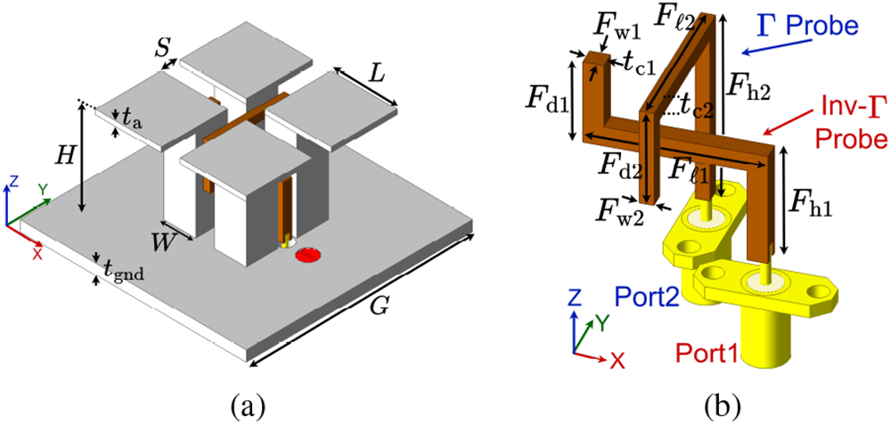
As depicted in Fig. 1a, the proposed MED antenna is composed of two pairs of metallic horizontal plates shorted by vertical posts, and a pair of mutually orthogonal feeding probes. Figure 1b shows the feeding network of the antenna. The first probe is inv- $\Gamma$ shaped while the second probe has the shape of
 $\Gamma$. Two SMA connectors connected to the feeding probes excite the antenna. Table 1 lists the dimensions of the proposed antenna.
Structure of the proposed (a) antenna 1 and (b) its feed network.

Figure 1 Long description
The structure of the proposed antenna, consisting of two pairs of metallic horizontal plates shorted by vertical posts. The plates are labeled S and L, while the posts are labeled H and W. A red dot is visible on the base labeled G. The image B illustrates the feed network of the antenna, featuring two probes. The first probe is labeled as inv-dash Gamma shaped and the second probe is labeled as Gamma shaped. The probes are connected to two ports, labeled Port1 and Port2. Various forces are labeled along the probes, including F subscript d1, F subscript d2, F subscript d3, F subscript d4, F subscript e1, F subscript e2, F subscript e3, F subscript e4, F subscript h1 and F subscript h2. The axes are marked with x, y and z directions, indicating orientation. The diagram provides a detailed view of the antenna′s structural and functional components.
Antenna dimensions in mm

Table 1 Long description
Dimensions in millimeters are given for an antenna body and two probe configurations labeled Inv Gamma Probe, MED Port 1, and Gamma Probe, MED Port 2. Under Antenna body, parameters L, S, H, G, W, t a, and t gnd have values 17.55, 4.97, 25.35, 60, 8.45, 1.3, and 2.8. For Inv Gamma Probe, MED Port 1, parameters t c1, F w1, F h1, F ell1, and F d1 have values 2.43, 2.36, 13.97, 21.43, and 10.5. For Gamma Probe, MED Port 2, parameters t c2, F w2, F h2, F ell2, and F d2 have values 2, 1.71, 23.08, 21.43, and 12. Port 2 has a larger F h value than Port 1, while both ports share the same F ell value of 21.43. The Port 1 thickness t c is 2.43 and the Port 2 thickness t c is 2.
Radiation and excitations principle
The metallic plates and posts serve as a pair of half-wave electric dipoles and shorted quarter-wave patches (acting as magnetic dipoles), respectively. Each feeding probe can be divided into three distinct sections [Reference Li and Luk6]:
(1) The first section is a vertical line that carries the signal from the input port to the horizontal section. This part functions like an air-filled stripline, with the probe serving as the inner conductor, the two posts as the ground plane, and air as the substrate. In the current design, the parameters
 $t_{\rm{c1,2}}$ and
$F_{\rm{w1,2}}$ represent the conductor widths and thicknesses of the equivalent striplines, respectively, while the parameter
$S$ denotes the substrate height. The conductor width and dielectric height primarily determine the characteristic impedance, while the conductor thickness has a secondary effect [Reference Pozar18].
(2) The second section is the horizontal line, which serves as the coupling element between the electric and magnetic dipoles. Since the resonators are coupled to each other via magnetic coupling, this section exhibits strong inductive behavior, which can potentially cause impedance mismatch in the antenna.
(3) The third and final section is another vertical line, designed as an open-ended stripline. It introduces a capacitive effect that compensates for the inductive effect from the previous section, helping to balance the overall impedance.


Ports isolation
To achieve high isolation between the antenna ports, the probe feeds should be placed as far apart as possible. Previous designs in the literature have used two orthogonal  $\Gamma$-shaped probe feeds [Reference Wu and Luk5–Reference Sun, Li and Xia7]. However, a limitation arises with the shorter probe: its open-ended section imposes a geometric constraint, as its first section cannot be shortened to increase the spacing between the feeds further. Therefore, we proposed an inv-
 $\Gamma$ shape probe. To further improve isolation, the magnetic dipole is designed to operate at the lower edge of the frequency band, allowing for a greater post height (
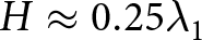 $H\approx 0.25\lambda_1$) and thereby increasing the spacing between the probes. Meanwhile, the electric dipole is designed at the center frequency, ensuring that the combined length of the plate and the gap is approximately
 $0.5\lambda_0$. The remaining design parameters are optimized to achieve a wide impedance bandwidth for both ports.
Simulation and analysis
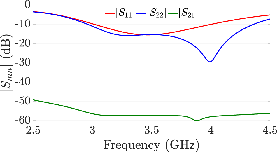
An electromagnetic (EM) full-wave simulation was executed utilizing Ansys® HFSS™ (High-Frequency Structure Simulator), which employs a finite element solver. Figure 2 illustrates the simulated S-parameters of antenna 1. The bandwidths for  $|S_{11}| \lt {-10}{dB}$ at port 1 and
 $|S_{22}| \lt {-10}{dB}$ at port 2 are in the ranges of 3 to 4 GHz and 2.96 to 4.36 GHz, respectively. Additionally, the broadband isolation exceeds 56 dB
S-parameters of antenna 1.

Upon examination of the reflection coefficient at the second port (i.e.,  $|S_{22}|$), two reflection zeros are apparent due to the coupling of the two resonators (electric and magnetic dipoles). However,
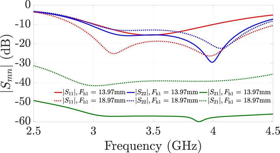
 $|S_{11}| \lt $ -10dB bandwidth of the first port is narrower than the second port, and the second reflection zero is not visible. From the theory of coupling, the reflection zeros are getting closer to each other, and finally, they cannot be distinguished when the coupling strength is weaker. The difference between the two ports, except for the shape, is the height of the probes. Figure 3 shows the S-parameters for different height of the first probe. The
 $|S_{11}| \lt $ -10 dB bandwidth is getting wider, and two reflection zeros are seen when the height is increased, which means the coupling strength between the dipoles is getting stronger. On the contrary, the isolation level is getting worse due to a reduction in the gap between the two probes. In other words, increasing the port height of the first probe not only increases the coupling strength between resonators (i.e., dipoles) but also increases the coupling between ports. Resulting in a wider
 $|S_{11}| \lt $ -10 dB bandwidth but weaker isolation.
 $|S_{22}|$ slightly differs due to the stronger interaction with the first probe.
Effect of the probe height on S-parameters of antenna 1.

Figure 3 Long description
The x-axis is labeled, Frequency (gigahertz), with tick labels at 2.5, 3, 3.5, 4 and 4.5. The y-axis is labeled, vertical bar S subscript m n vertical bar (decibel), with tick labels at 0, minus 10, minus 20, minus 30, minus 40, minus 50 and minus 60. A legend inside the plot lists six series: vertical bar S subscript 11 vertical bar, F subscript h 1 equals 13.97 millimeter; vertical bar S subscript 11 vertical bar, F subscript h 1 equals 18.97 millimeter; vertical bar S subscript 22 vertical bar, F subscript h 1 equals 13.97 millimeter; vertical bar S subscript 22 vertical bar, F subscript h 1 equals 18.97 millimeter; vertical bar S subscript 21 vertical bar, F subscript h 1 equals 13.97 millimeter; vertical bar S subscript 21 vertical bar, F subscript h 1 equals 18.97 millimeter. All curves start near the top of the plot close to 0 decibel at 2.5 gigahertz. The vertical bar S subscript 11 vertical bar curves descend to a dip near about 3.1 gigahertz and then rise toward 4.5 gigahertz, ending near about minus 10 decibel. The vertical bar S subscript 22 vertical bar curves show a deeper dip near about 4.0 gigahertz, reaching near about minus 30 decibel, then rise toward 4.5 gigahertz. The vertical bar S subscript 21 vertical bar curves remain much lower than the others across the full frequency range, staying between about minus 30 decibel and minus 60 decibel, with the lowest point near about 4.0 gigahertz close to minus 60 decibel.
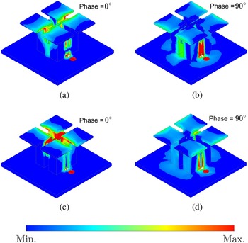
To elucidate the operating mechanism of the proposed antenna, Fig. 4 depicts the magnitude of the simulated current distribution when port 1 and port 2 are excited individually at the center frequency of 3.5 GHz. Fig. 4a and 4c show the magnitude of the currents on the posts and slot edge of the plates within the aperture attain maximum strength at phase = 0 $^{\circ}$, which indicates that the magnetic dipole is excited. At a phase of 90
 $^{\circ}$, the currents on the plates at the surrounding edges reach their maximum strength, indicating that the electric dipole is excited (Fig. 4b and 4d). As seen, the complementary sources are excited consecutively, which provides a hemispherical radiation pattern.
Magnitude surface current distribution of antenna 1 at 3.5 GHz when (a)–(b) port 1 and (c)–(d) port 2 are excited, respectively.

Figure 4 Long description
Four 3D antenna model renderings display the surface current magnitude distribution at 3.5 gigahertz. Each panel shows the antenna geometry colored by current magnitude using a continuous colormap scale ranging from minimum to maximum, where minimum represents the lowest current level and maximum represents the highest. No spatial axis labels or units are shown in the figure; the colormap solely indicates relative current magnitude intensity across the antenna structure. The colorbar at the bottom of the composite figure is labeled Min. on the left and Max. on the right, indicating a normalized relative scale rather than absolute values in specific units. Port 1 excited at phase equals 0 degrees: Current magnitude reaches its highest relative level concentrated at the posts and along the slot edges of the plates within the aperture region. The surrounding perimeter edges show comparatively lower magnitude. Port 1 excited at phase equals 90 degrees: The highest relative current magnitude shifts to the plates at the surrounding perimeter edges. The posts and slot edge region shows reduced magnitude compared to the 0 degree case. Port 2 excited at phase equals 0 degrees: The distribution pattern closely mirrors the port 1 at 0 degree case, with peak relative current magnitude at the posts and slot edges within the aperture. Surrounding edges carry lower magnitude. Port 2 excited at phase equals 90 degrees: Similar to the port 1 at 90 degree case, the highest relative magnitude appears along the surrounding perimeter edges, while the posts and slot edge region shows lower magnitude. Across both ports, the shared pattern is consistent: phase equals 0 degrees concentrates current near the feed posts and slot edges, while phase equals 90 degrees redistributes current toward the surrounding perimeter edges. No absolute numeric peak values are indicated in the figure; only relative intensity levels are visually distinguishable through the colormap.
Consequently, the equivalent electric and magnetic currents exhibit a 90 $^{\circ}$ phase difference (Fig.5) and are orthogonal to each other, resulting in a wider impedance bandwidth and reduced back radiation [Reference Li and Luk6].
Vector surface current distribution of antenna 1 when port 1 is excited at 3.5 GHz, phase = (a) 0 $^{\circ}$, (b) 90
 $^{\circ}$, (c) 180
 $^{\circ}$, (d) 270
 $^{\circ}$.

Figure 5 Long description
Vector surface current distribution of antenna 1 with port 1 excited at 3.5 GHz, shown at four excitation phase snapshots: 0 degrees, 90 degrees, 180 degrees and 270 degrees. The figure is a spatial field map over the antenna surface with no labeled coordinate axes. Arrows encode the direction and relative magnitude of surface current vectors at each point on the antenna surface. The colormap encodes the magnitude of surface current density, with units not specified in the figure. The colorbar below all four panels ranges from Min at the left end to Max at the right end, with no intermediate numeric tick values visible. At phase 0 degrees: a strong, narrow vertical band of high-magnitude current vectors runs centrally along the antenna surface, with minimal activity at the outer regions. At phase 90 degrees: the central vertical band persists with comparable density and small clusters of vectors appear at the sides of the central region. At phase 180 degrees: the central band remains dominant but shifts slightly off-center, with a more pronounced side cluster visible adjacent to the main band. At phase 270 degrees: the distribution returns to a pattern closely resembling phase 0 degrees, with a strong central vertical band and reduced peripheral activity. Across all four snapshots, the highest current density concentrates along a central vertical strip of the antenna surface, with minor redistributions occurring as the excitation phase advances from 0 to 270 degrees.
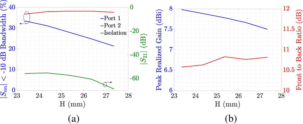
Figure 6 illustrates the advantages and disadvantages of using a higher post, as reflected in the S-parameters (Fig. 6a) and radiation performance (Fig. 6b). The fractional bandwidth of the first port becomes narrower as the post height increases. This occurs because the coupling between the electric and magnetic dipoles – already weak for the first probe – further decreases. The effect is less pronounced for the second port, and the isolation at the center frequency improves slightly. On the other hand, increasing the post height slightly reduces the peak realized gain, since the magnetic dipole resonance frequency shifts to a lower value, while the front-to-back ratio remains nearly unchanged.
Effect of post height  $H$ on (a) S-parameters and (b) radiation at 3.5 GHz.

Figure 6 Long description
Three line series versus H in millimeter. The x-axis is labeled, H (mm), with ticks at 23, 24, 25, 26, 27, 28. The left y-axis is labeled, vertical bar S subscript m n vertical bar less than minus 10 decibel Bandwidth (percent), with ticks at 0, 10, 20, 30, 40. The right y-axis is labeled, vertical bar S subscript 2 1 vertical bar (dB), with ticks at 0, minus 20, minus 40, minus 60. A legend lists Port 1, Port 2, Isolation. Port 1 is a line that starts near 33 percent at H about 23.5 millimeter and decreases to about 21 percent at H about 27 millimeter. Port 2 is a line near 37 to 38 percent across the range, rising slightly from about 37 percent near H about 23.5 millimeter to about 38 percent near H about 25 to 26 millimeter, then slightly decreasing to about 37.5 percent near H about 27 millimeter. Isolation is a line near minus 55 decibel at H about 23.5 millimeter, near minus 54 decibel at H about 24 millimeter, near minus 55 decibel at H about 25 millimeter, near minus 57 decibel at H about 26 millimeter and near minus 62 decibel at H about 27 millimeter. The image B showing two line series versus H in millimeter. The x-axis is labeled, H (mm), with ticks at 23, 24, 25, 26, 27, 28. The left y-axis is labeled, Peak Realized Gain (dBi), with ticks at 6, 6.5, 7, 7.5, 8. The right y-axis is labeled, Front to Back Ratio (dB), with ticks at 10, 10.5, 11, 11.5, 12. The gain line starts near 8.0 at H about 23.5 millimeter and decreases to about 7.5 at H about 27 millimeter, passing about 7.9 near 24 millimeter, about 7.8 near 25 millimeter and about 7.65 near 26 millimeter. The front to back ratio line starts near 10.55 at H about 23.5 millimeter, is near 10.6 at H about 24.5 millimeter, rises to about 10.8 at H about 25.5 millimeter, is near 10.75 at H about 26.5 millimeter and is near 10.8 at H about 27.5 millimeter.
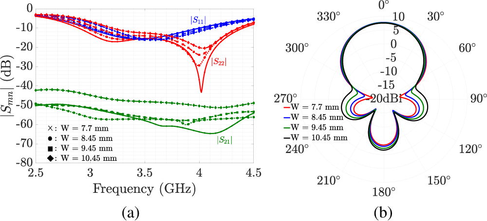
Similarly, Fig. 7a shows the effect of varying post widths on the S-parameters. The fractional bandwidth becomes narrower, and the isolation weakens as the post width increases. Furthermore, a larger post width increases the side-lobe level and slightly reduces the front-to-back ratio, as illustrated in Fig. 7b.
Effect of post width  $W$ on (a) S-parameters and (b) H-plane radiation of port 2 at 3.5 GHz.

Figure 7 Long description
A line graph with three labeled traces, S subscript 11, S subscript 22 and S subscript 21, each drawn as four line styles for W equals 7.7 millimeter, 8.45 millimeter, 9.45 millimeter and 10.45 millimeter. The horizontal axis is labeled, Frequency in gigahertz, from 2.5 to 4.5 with labeled ticks at 2.5, 3, 3.5, 4 and 4.5. The vertical axis is labeled, vertical bar S subscript m n vertical bar in decibel, from 0 at the top down to minus 80 at the bottom, with labeled ticks every 10 decibel. The S subscript 11 group is plotted near the top, starting near about minus 5 decibel at 2.5 gigahertz, dipping to around the mid minus teens between about 3.2 and 3.6 gigahertz, then rising toward about minus 5 to minus 8 decibel by 4.5 gigahertz. The S subscript 22 group shows a pronounced dip near 4.0 gigahertz, with one curve reaching roughly the mid minus 40 decibel range at the minimum, while the other W curves dip less deeply, around the minus 20 to minus 30 decibel range, then rise toward about minus 10 decibel by 4.5 gigahertz. The S subscript 21 group is plotted lower, around minus 40 to minus 70 decibel across the band, with curves generally decreasing from about the mid minus 40 to minus 50 decibel range near 2.5 gigahertz to minima around the low to mid minus 60 decibel range between about 3.5 and 4.2 gigahertz, then rising slightly toward 4.5 gigahertz. A legend inside the plot lists the four W values with marker symbols. The image B showing a polar plot with angle labels around the circle at 0 degree, 30 degree, 60 degree, 90 degree, 120 degree, 150 degree, 180 degree, 210 degree, 240 degree, 270 degree, 300 degree and 330 degree. The radial scale is labeled at 10, 5, 0, minus 5, minus 10 and minus 15, with a central label reading 20 decibel. Four overlaid radiation patterns correspond to W equals 7.7 millimeter, 8.45 millimeter, 9.45 millimeter and 10.45 millimeter as listed in the legend. The patterns form a main lobe centered near 0 degree with a rounded top and smaller lobes around the lower half near 180 degree, with the four curves closely spaced and differing slightly in the size of the side lobes.
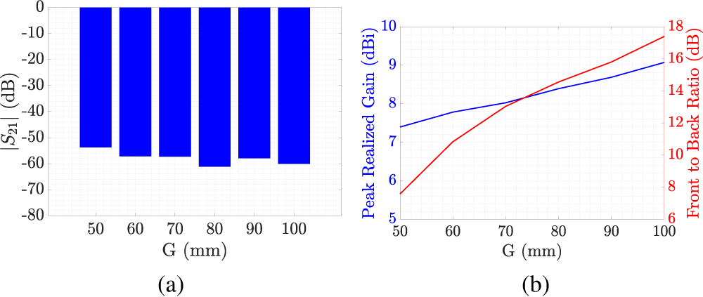
Figure 8 demonstrates that the antenna gain can be increased and the front-to-back ratio improved by enlarging the ground plane, without degrading the isolation performance. However, increasing the ground plane size may lead to the appearance of grating lobes in an array configuration, since the antenna spacing exceeds half a wavelength.
Effect of ground plane size  $G$ on (a) isolation and (b) radiation at 3.5 GHz.

Figure 8 Long description
A showing a bar chart. The horizontal axis label is, G (millimeter), with tick labels 50, 60, 70, 80, 90, 100. The vertical axis label is, vertical bar S subscript 21 vertical bar (decibel), with tick labels 0, minus 10, minus 20, minus 30, minus 40, minus 50, minus 60, minus 70, minus 80. The bar values at each G are: 50 is about minus 55 decibel, 60 is about minus 58 decibel, 70 is about minus 58 decibel, 80 is about minus 62 decibel, 90 is about minus 59 decibel, 100 is about minus 61 decibel. B showing a two line graph with two vertical axes. The horizontal axis label is, G (millimeter), with tick labels 50, 60, 70, 80, 90, 100. The left vertical axis label is, Peak Realized Gain (decibel i), with tick labels 5, 6, 7, 8, 9, 10. The right vertical axis label is, Front to Back Ratio (decibel), with tick labels 6, 8, 10, 12, 14, 16, 18. The Peak Realized Gain line values are approximately: at 50 is 7.4, at 60 is 7.8, at 70 is 8.0, at 80 is 8.3, at 90 is 8.6, at 100 is 9.0. The Front to Back Ratio line values are approximately: at 50 is 7.5, at 60 is 11.0, at 70 is 13.5, at 80 is 15.0, at 90 is 16.0, at 100 is 17.5.
It is observed that the main parameter influencing the isolation is the gap between the two probes. This gap can be adjusted by increasing the height of the second probe or decreasing that of the first probe. However, since the second probe is already at the limit of the post height, it cannot be increased further. Otherwise, the horizontal section of the probe – which acts as the coupling section between the dipoles – would extend above the antenna, resulting in impedance mismatch.
Probe orthogonality
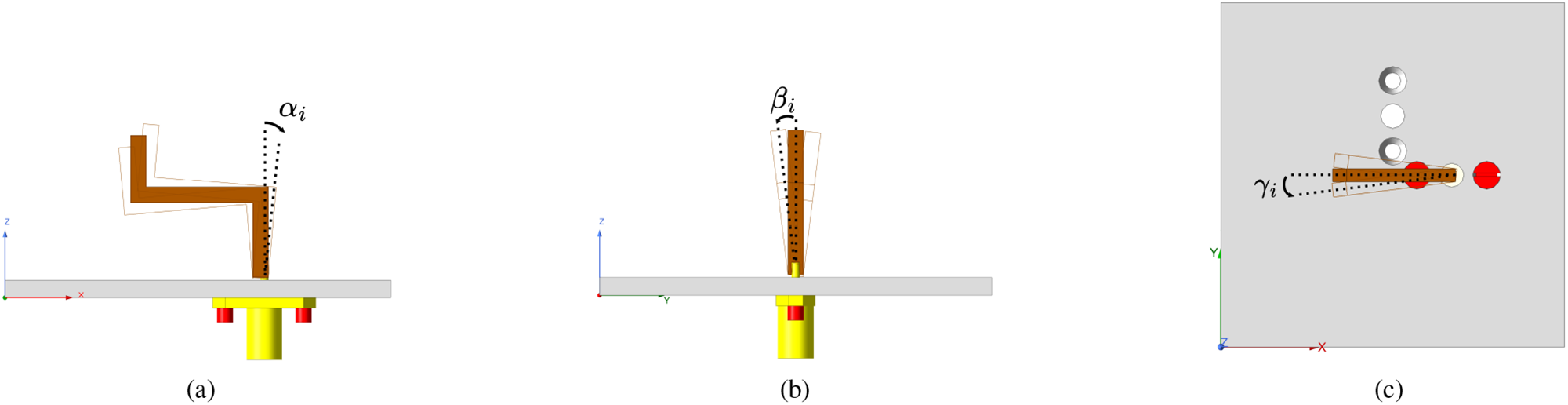
The probes’ alignment might be slightly offset during assembly of the proposed antenna, e.g., during soldering to the SMA connectors. To investigate the effect of probe misalignment, three misalignment angles are defined. Figure 9a shows the pitch misalignment angle that represents the rotation around the y-axis for port 1 (x-axis for port 2), and it is indicated as  $\alpha_i$ where the subscript
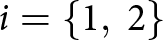 $i = \{1, \: 2\}$ shows the probe ID. Similarly, the rotation around the x-axis for port 1 (y-axis for port 2) represents the roll misalignment,
 $\beta_i$, as shown in Fig. 9b. Finally, the yaw misalignment (rotation around the z-axis) is defined by
 $\gamma_i$ (Fig. 9c).
Probe misalignment angles (a) pitch, (b) roll, and (c) yaw.

Figure 10 shows the effects of pitch, roll, and yaw misalignment within a range of  $\pm 2^\circ$ on port-to-port isolation, cross polarization isolation (XPI) (i.e.,
 $|S_{21}|$) for the first and second probe separately. Only one misalignment is varied at a time, while the others are kept at 0
 $^{\circ}$. Figure 10a shows that the pitch misalignment does not significantly affect
 $|S_{21}|$; the port isolation remains above 50 dB within the operating bandwidth. On the other hand, a roll misalignment significantly degrades isolation performance. It drops by almost 30dB at 2
 $^{\circ}$ of misalignment as shown in Fig. 10b. The yaw misalignment has the most significant effect on port isolation, even with an error of only 0.5
 $^{\circ}$, the port isolation decreases by approximately 23 dB (Fig. 10c).
Individual effects of (a) pitch, (b) roll, and (c) yaw misalignment on  $|S_{21}|$ for each probe.

Figure 10 Long description
A line graph with the y-axis labeled, vertical bar S subscript 21 vertical bar, open parenthesis decibel close parenthesis, ranging from minus 80 to 0 in increments of 10. The x-axis is labeled, Frequency, open parenthesis gigahertz close parenthesis, ranging from 2.5 to 4.5 with labeled ticks at 2.5, 3, 3.5, 4 and 4.5. A legend lists alpha subscript 1 equals minus 2 degrees, minus 1.5 degrees, minus 1 degrees, minus 0.5 degrees, 0 degrees, 0.5 degrees, 1 degrees, 1.5 degrees, 2 degrees and alpha subscript 2 equals minus 2 degrees, minus 1.5 degrees, minus 1 degrees, minus 0.5 degrees, 0 degrees, 0.5 degrees, 1 degrees, 1.5 degrees, 2 degrees. Multiple solid and dotted curves start near about minus 45 to minus 50 at 2.5 gigahertz, then several curves dip between about 3.0 and 3.2 gigahertz to values between about minus 60 and minus 80 and then rise toward about minus 55 to minus 60 by 4.5 gigahertz. One curve shows a deep notch near about 3.9 to 4.0 gigahertz reaching about minus 80. The image B showing a line graph with the y-axis labeled, vertical bar S subscript 21 vertical bar, open parenthesis decibel close parenthesis, ranging from minus 80 to 0 in increments of 10. The x-axis is labeled, Frequency, open parenthesis gigahertz close parenthesis, ranging from 2.5 to 4.5 with labeled ticks at 2.5, 3, 3.5, 4 and 4.5. A legend lists beta subscript 1 equals minus 2 degrees, minus 1.5 degrees, minus 1 degrees, minus 0.5 degrees, 0 degrees, 0.5 degrees, 1 degrees, 1.5 degrees, 2 degrees and beta subscript 2 equals minus 2 degrees, minus 1.5 degrees, minus 1 degrees, minus 0.5 degrees, 0 degrees, 0.5 degrees, 1 degrees, 1.5 degrees, 2 degrees. Several curves lie between about minus 25 and minus 40 from 2.5 to about 4.0 gigahertz, then many slope downward after about 4.0 gigahertz toward about minus 35 to minus 55 by 4.5 gigahertz. One lower curve runs near about minus 50 at 2.5 gigahertz, drops toward about minus 60 around 3.2 to 3.6 gigahertz and remains near about minus 55 to minus 60 through 4.5 gigahertz. The image C showing a line graph with the y-axis labeled, vertical bar S subscript 21 vertical bar, open parenthesis decibel close parenthesis, ranging from minus 80 to 0 in increments of 10. The x-axis is labeled, Frequency, open parenthesis gigahertz close parenthesis, ranging from 2.5 to 4.5 with labeled ticks at 2.5, 3, 3.5, 4 and 4.5. A legend lists gamma subscript 1 equals minus 2 degrees, minus 1.5 degrees, minus 1 degrees, minus 0.5 degrees, 0 degrees, 0.5 degrees, 1 degrees, 1.5 degrees, 2 degrees and gamma subscript 2 equals minus 2 degrees, minus 1.5 degrees, minus 1 degrees, minus 0.5 degrees, 0 degrees, 0.5 degrees, 1 degrees, 1.5 degrees, 2 degrees. Most curves form a band between about minus 20 and minus 35 across 2.5 to 4.5 gigahertz with gentle curvature. A lower curve starts near about minus 50 at 2.5 gigahertz, decreases to around minus 60 near about 3.9 to 4.0 gigahertz and then rises slightly toward about minus 55 by 4.5 gigahertz.
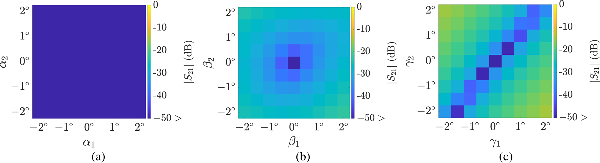
Furthermore, Fig. 11 illustrates the individual effects of misalignment angles (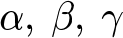 $\alpha,\: \beta,\: \gamma$) on
 $|S_{21}|$ with simultaneous angle variation on both probes at 3.5 GHz. The difference in impact can be attributed to the orthogonality and relative positioning of the probes. Since probe 1 lies in the xz-plane and probe 2 lies in the yz-plane, their orthogonality can be evaluated by examining the scalar (dot) product of their unit normal vectors. Assuming that the unit normal vector of probe 1 is given by
 $\hat{a}_{\rm{n}1} = [0,\: 1,\: 0]'$ and that of probe 2 by
 $\hat{a}_{\rm{n}2} = [1,\: 0,\: 0]'$, three cases can be analyzed as follows:
Individual effects of (a) pitch, (b) roll, and (c) yaw misalignment on  $|S_{21}|$ with simultaneous angle variation on both probes at 3.5 GHz.

Figure 11 Long description
A heatmap with horizontal axis label, alpha subscript 1 and vertical axis label, alpha subscript 2. Both axes show tick labels from minus 2 degrees to 2 degrees. A vertical scale bar at the right is labeled, vertical bar S subscript 21 vertical bar, open parenthesis decibel close parenthesis, with tick labels 0, minus 10, minus 20, minus 30, minus 40, minus 50. The scale bar indicates that values nearer 0 decibel correspond to higher vertical bar S subscript 21 vertical bar and values nearer minus 50 decibel correspond to lower vertical bar S subscript 21 vertical bar. The heatmap field appears nearly uniform, with no distinct bands or localized regions. The image B showing a heatmap with horizontal axis label, beta subscript 1 and vertical axis label, beta subscript 2. Both axes show tick labels from minus 2 degrees to 2 degrees. A vertical scale bar at the right is labeled, vertical bar S subscript 21 vertical bar, open parenthesis decibel close parenthesis, with tick labels 0, minus 10, minus 20, minus 30, minus 40, minus 50. The scale bar indicates that values nearer 0 decibel correspond to higher vertical bar S subscript 21 vertical bar and values nearer minus 50 decibel correspond to lower vertical bar S subscript 21 vertical bar. The heatmap shows a localized region centered near beta subscript 1 equals 0 degrees and beta subscript 2 equals 0 degrees, with surrounding square like bands expanding outward from the center. The image C showing a heatmap with horizontal axis label, gamma subscript 1 and vertical axis label, gamma subscript 2. Both axes show tick labels from minus 2 degrees to 2 degrees. A vertical scale bar at the right is labeled, vertical bar S subscript 21 vertical bar, open parenthesis decibel close parenthesis, with tick labels 0, minus 10, minus 20, minus 30, minus 40, minus 50. The scale bar indicates that values nearer 0 decibel correspond to higher vertical bar S subscript 21 vertical bar and values nearer minus 50 decibel correspond to lower vertical bar S subscript 21 vertical bar. The heatmap shows a diagonal band running from the lower left toward the upper right, crossing near gamma subscript 1 equals 0 degrees and gamma subscript 2 equals 0 degrees, with block like regions on either side of the diagonal.
1) Pitch misalignment: In this case, the probes rotate around the direction of their normal vectors. As a result, the unit normal vectors remain unchanged, and the probes remain orthogonal regardless of the values of  $\alpha_1$ and
 $\alpha_2$. Although the vertical gap between the probes changes slightly, its impact is negligible within the examined misalignment range, and the isolation remains above 50 dB in all combinations (Fig. 11a).
2) Roll misalignment: Probe 1 is rotating  $\beta_1$ degrees around the x-axis, and probe 2 is rotating
 $\beta_2$ degrees around the y-axis. The normal unit vectors of the new planes can be found by applying the rotation matrix as
 \begin{equation}
\hat{a}^\prime _{\rm{n}1} =
\begin{bmatrix}
1 & 0 & 0 \\
0 & \cos\beta_1 & -\sin\beta_1 \\
0 & \sin\beta_1 & \cos\beta_1
\end{bmatrix}
\begin{bmatrix}
0 \\
1 \\
0
\end{bmatrix} =
\begin{bmatrix}
0 \\
\cos\beta_1 \\
\sin\beta_1
\end{bmatrix} \text{,}
\end{equation}
 \begin{equation}\hspace{25pt}
\hat{a}^\prime _{\rm{n}2} =
\begin{bmatrix}
\cos\beta_2 & 0 & \sin\beta_2 \\
0 & 1 & 0 \\
-\sin\beta_2 & 0 & \cos\beta_2
\end{bmatrix}
\begin{bmatrix}
1 \\
0 \\
0
\end{bmatrix} =
\begin{bmatrix}
\cos\beta_2 \\
0 \\
-\sin\beta_2
\end{bmatrix} \text{.}
\end{equation}
 \begin{equation}
\hat{a}^\prime _{\rm{n}1} \cdot \hat{a}^\prime _{\rm{n}2} = -\sin\beta_1 \sin\beta_2\text{,}
\end{equation}
which indicates that the probes are not orthogonal iff 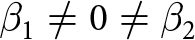 $\beta_1 \neq 0 \neq \beta_2$, since the scalar product is not zero. As shown in Fig. 11b, the isolation level decreases consistently regardless of the direction of rotation, and the behavior is nearly symmetrical around both axes. This is because the distance between the probes decreases by the same amount, whether rotated in the positive or negative direction. However, a special case occurs when the probes are orthogonal, i.e., when
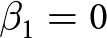 $\beta_1 = 0$ or
 $\beta_2 = 0$. Even in these cases, isolation continues to degrade, although orthogonality is maintained. This is due to the relative placement of the probes – specifically, the rotated probe becomes physically closer to the fixed probe, which increases the coupling between them.
3) Yaw misalignment: In this case, both probes are rotating around the z-axis by  $\gamma_1$ and
 $\gamma_2$, respectively. The normal unit vectors of the new planes are
 \begin{equation}\hspace{23pt}
\hat{a}^\prime _{\rm{n}1} =
\begin{bmatrix}
\cos\gamma_1 & -\sin\gamma_1 & 0 \\
\sin\gamma_1 & \cos\gamma_1 & 0\\
0 & 0 & 1
\end{bmatrix}
\begin{bmatrix}
0 \\
1 \\
0
\end{bmatrix} =
\begin{bmatrix}
-\sin\gamma_1 \\
\cos\gamma_1 \\
0
\end{bmatrix} \text{,}
\end{equation}
 \begin{equation}
\hat{a}^\prime _{\rm{n}2} =
\begin{bmatrix}
\cos\gamma_2 & -\sin\gamma_2 & 0 \\
\sin\gamma_2 & \cos\gamma_2 & 0\\
0 & 0 & 1
\end{bmatrix}
\begin{bmatrix}
1 \\
0 \\
0
\end{bmatrix} =
\begin{bmatrix}
\cos\gamma_2 \\
\sin\gamma_2 \\
0
\end{bmatrix} \text{.}
\end{equation}
 \begin{equation}
\hat{a}^\prime _{\rm{n}1} \cdot \hat{a}^\prime _{\rm{n}2} = \cos\gamma_1 \sin\gamma_2 - \sin\gamma_1 \cos\gamma_2 .
\end{equation}
It states that the probes remain orthogonal iff 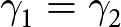 $\gamma_1=\gamma_2$. The degradation in isolation is expected to be smaller than in the previous case when orthogonality is maintained, since the relative positions of the probes remain the same (i.e., the distance between the probes remains unchanged). Figure 11c demonstrates that the isolation remains nearly the same for identical combinations of misalignment angles (
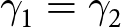 $\gamma_1=\gamma_2$). Moreover, it depends on the direction of rotation and exhibits symmetry around the diagonal. In the worst case, the third sections of the probes come very close to each other, resulting in an isolation level of approximately 14dB.
Final design
The importance of orthogonality and the relative positioning of the probes was examined in the previous section. To minimize probe misalignment across the three analyzed cases with a simple and effective approach, four plastic (Nylon PA12) support rods (1mm of diameter) are inserted through the metallic posts and probe feeds to hold the feeding structure in place. Figure 12 shows the feed networks of the two antennas and their performance. The operating mechanism of the proposed antenna remains unchanged, and a slight improvement is obtained in isolation.
Comparison between antenna 1 (initial design) and antenna 2 (final design).

Figure 12 Long description
Two rows labeled Ant.1 and Ant.2 and four columns labeled Feed Network, Complex Mag. of Current Dist. at 3.5 GHz, S-parameters and Realized Gain. In the Feed Network column, the top row shows a 3D structure with two labeled ports, Port1 and Port2 and a small axis triad labeled X, Y and Z. The bottom row shows a similar 3D structure with Port1 and Port2 labels and the same X, Y and Z axis triad. In the Complex Mag. of Current Dist. at 3.5 GHz column, the top row shows a 3D field plot over a square base with a raised central structure and four top elements. The bottom row shows a similar 3D field plot with the same overall geometry. In the S-parameters column, each row contains a line graph. The x-axis is labeled Frequency (GHz), ranging from 2.5 to 4.5. The y-axis is labeled magnitude of S parameter (dB), ranging from 0 to minus 80. A legend lists magnitude of S subscript 11, magnitude of S subscript 22 and magnitude of S subscript 21. In the top row, the magnitude of S subscript 21 curve is near minus 50 to minus 60 across the band and the magnitude of S subscript 11 and magnitude of S subscript 22 curves lie between about 0 and minus 30 with a pronounced dip near about 4.0 gigahertz. In the bottom row, the magnitude of S subscript 21 curve drops from about minus 50 toward about minus 70 near mid band and rises toward about minus 60 by 4.5 gigahertz, while the magnitude of S subscript 11 and magnitude of S subscript 22 curves remain between about 0 and minus 30 with a dip near about 4.0 gigahertz. In the Realized Gain column, each row contains a line graph. The x-axis is labeled Frequency (GHz), ranging from 2.5 to 4.5. The y-axis is labeled Realized Gain (dBi), ranging from 0 to 10. A legend lists Port1 and Port2. In the top row, both Port1 and Port2 rise from about 3 at 2.5 gigahertz to about 8 near 3.0 gigahertz, stay near about 8 through around 4.0 gigahertz, then dip slightly near about 4.2 gigahertz and end near about 7 to 8 at 4.5 gigahertz. In the bottom row, both Port1 and Port2 rise from about 2 to 3 at 2.5 gigahertz to about 8 near 3.0 gigahertz, remain near about 8 through around 4.0 gigahertz and end near about 7 to 8 at 4.5 gigahertz.
Experimental results and discussion
Fabrication and assembly
Figure 13a shows the fabricated parts of the proposed antenna. The body of the antenna is made of low-cost, standard metal 3D-printed aluminum alloy (AlSi $_10$Mg) with a machine tolerance of
 $\pm$0.2mm. The manufacturing constraints for this material include a minimum feature size of 0.4mm and a minimum wall thickness of 1mm. The white support rods are 3D-printed Nylon (PA12), while the probes are milled from brass. A WR-SMA Panel Jack 2-Hole Flange Connector is used to feed the antenna ports, and stainless steel DIN 963 slotted countersunk screws are used for connector mounting.
Fabricated antenna (a) un-assembled and (b) assembled.

Simulated and measured S-parameters.

Figure 14 Long description
The y-axis label is, vertical bar S subscript m n vertical bar, in decibel, ranging from 0 to minus 80. The y-axis tick labels are 0, minus 10, minus 20, minus 30, minus 40, minus 50, minus 60, minus 70 and minus 80. The x-axis label is Frequency, in gigahertz, ranging from 2.5 to 4.5 with tick labels 2.5, 3, 3.5, 4 and 4.5. A legend inside the plot lists six series: vertical bar S subscript 11 vertical bar, sim.; vertical bar S subscript 11 vertical bar, meas.; vertical bar S subscript 22 vertical bar, sim.; vertical bar S subscript 22 vertical bar, meas.; vertical bar S subscript 21 vertical bar, sim.; vertical bar S subscript 21 vertical bar, meas. The vertical bar S subscript 11 vertical bar simulated trace starts near about minus 3 at 2.5 gigahertz, decreases to around minus 15 by about 3.3 to 3.6 gigahertz, then rises toward about minus 6 by 4.5 gigahertz. The vertical bar S subscript 11 vertical bar measured trace follows a similar path, with points around minus 3 at 2.5 gigahertz, around minus 15 near about 3.4 to 3.6 gigahertz and around minus 7 to minus 8 near 4.5 gigahertz. The vertical bar S subscript 22 vertical bar simulated trace starts near about minus 3 at 2.5 gigahertz, drops to around minus 15 near about 3.3 to 3.6 gigahertz, then forms a deep notch near 4.0 gigahertz reaching roughly the mid minus 30s and rises again toward about minus 8 by 4.5 gigahertz. The vertical bar S subscript 22 vertical bar measured trace is similar but with a deeper notch slightly above 4.0 gigahertz, reaching roughly around minus 40, then rising toward about minus 10 by 4.5 gigahertz. The vertical bar S subscript 21 vertical bar simulated trace is between about minus 45 and minus 70 across the band, decreasing from roughly the high minus 40s near 2.5 gigahertz to a minimum near about 3.6 gigahertz around minus 70, then increasing to roughly around minus 60 by 4.5 gigahertz. The vertical bar S subscript 21 vertical bar measured trace begins around the low minus 50s near 2.5 gigahertz, decreases to around minus 70 near about 3.5 to 3.6 gigahertz, then increases to around minus 45 by 4.5 gigahertz.
To avoid plastic deformation during the soldering process, four metal rods were temporarily 3D printed and installed in place of the plastic supports to ensure mechanical stability. These metal rods were later replaced with the final plastic ones after soldering was completed. The assembled prototype is shown in Fig.13b.
Antenna measurements
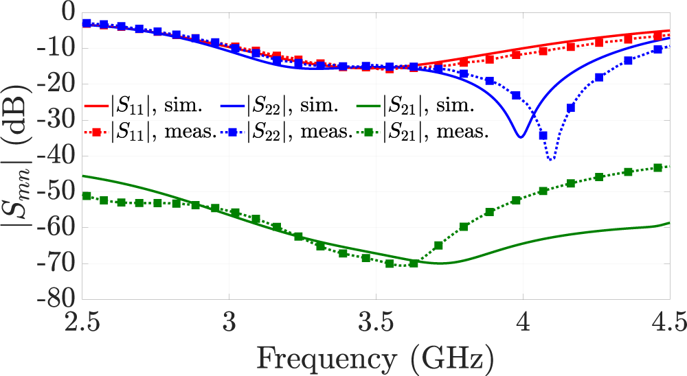
Figure 14 depicts the simulated and measured S-parameters of the proposed antenna. The simulated and measured  $|S_{11}| \lt $ -10 dB bandwidths are approximately 3.02 to 4GHz (28%) and 3.05 to 4.13GHz (30%), respectively. Similarly, the
 $|S_{22}| \lt $ -10 dB bandwidths are around 2.97 to 4.35GHz (38%, simulated) and 3.03 to 4.46GHz (38%, measured). The corresponding isolation remains above 50 dB throughout the operating bandwidth. Notably, the measured isolation reaches approximately 70dB at 3.5 GHz. It is observed that the measured and simulated results show good agreement, with a slight frequency shift attributed to fabrication tolerances.
To measure the radiation pattern and broadside realized gain of the proposed antenna, the measurement setup was arranged using absorber walls as shown in Fig. 15b. An MVG QH2000 open-boundary quad-ridge horn antenna served as the reference antenna. Since both antennas are dual-polarized, a full four-port measurement was performed using R&S®ZVA24 vector network analyzer (VNA) to capture the co-polarized and cross-polarized components for each polarization state. Prior to measurement, the VNA was calibrated using the short–open–load–thru (SOLT) method to compensate for systematic errors introduced by cables and connectors, utilizing an electronic calibration kit R&S®ZV-Z52. Figure 15a illustrates the measurement diagram. The distance between the MED antenna – antenna under test (AUT) – and the reference antenna was set to 50cm, which exceeds the far-field criterion. We then accounted for the reference antenna gain and the 50cm free-space path loss to report the AUT’s absolute gain values. The reference antenna and the AUT were precisely aligned using a laser system to minimize pointing errors.
Measurement setup (a) diagram and (b) view of the setup.

Figure 15 Long description
Two parts are shown. The first part is a diagram illustrating the measurement setup for antenna testing. On the left side, labeled as AUT, is the antenna under test, with a position stage labeled RS. The distance between the AUT and the reference antenna, labeled RA, is marked as 50 centimeters. The RA is positioned on the right side. Below the RA, a vector network analyzer labeled VNA is connected to a PC. The VNA has four ports labeled P1, P2, P3 and P4, corresponding to numbers 1, 2, 3 and 4. The diagram includes labels for each component, such as the reference antenna model and the vector network analyzer model. The second part of the image shows a real-world view of the setup. It features a room with absorber walls, which are blue and have a triangular pattern. In the center, equipment is set up, including antennas and cables, reflecting the arrangement shown in the diagram. The setup is designed to measure the radiation pattern and gain of the antenna under test.
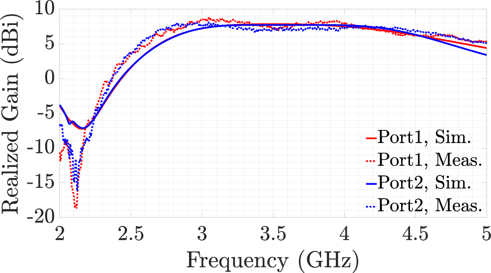
Figure 16 shows the simulated and measured broadside realized gains. The measured realized gains for both ports vary from 7.2 to 7.9 dBi, and the proposed antenna exhibits nearly flat broadside gain over its operating bandwidth. The average measured antenna efficiencies are 86% and 90% for the first port and second port, respectively. The simulated and measured radiation patterns of the proposed antenna are shown in Fig. 17. The measured half-power beamwidths in the E-plane are 59 $^{\circ}$, 62
 $^{\circ}$, and 64
 $^{\circ}$ for the first port and 89
 $^{\circ}$, 80
 $^{\circ}$, and 89
 $^{\circ}$ for the second port at 3, 3.5, and 4GHz, respectively. The measured half-power beamwidths in the H-plane are 85
 $^{\circ}$, 78
 $^{\circ}$, and 83
 $^{\circ}$ for the first port and 58
 $^{\circ}$, 62
 $^{\circ}$, and 63
 $^{\circ}$ for the second port at 3, 3.5, and 4GHz, respectively. The measured cross-polarization discrimination (XPD) is more than 20dB at all frequency points. The measured values are slightly stronger than the simulated ones, which might be due to the tilting error in the placement of the reference antenna.
Simulated and measured broadside realized gains.

Simulated and measured normalized gain patterns for port 1 in (a), (c), and (e), and for port 2 in (b), (d), and (f), at 3, 3.5, and 4GHz, respectively.

Figure 17 Long description
Simulated and measured normalized gain patterns for two ports at frequencies of 3, 3.5 and 4 GHz are displayed. Each plot shows E-plane and H-plane patterns. The radial axis represents gain magnitude in decibels, with concentric circles at minus 20, minus 40 and minus 60 decibels. G theta and G phi represent polarization components. For Port 1, the E-plane shows main lobes around 0 and 180 degrees, with close agreement between simulated and measured patterns. The H-plane reveals multi-lobed structures with notable nulls around 90 and 270 degrees. For Port 2, the E-plane patterns also align well, with main lobes near 0 and 180 degrees. The H-plane shows more pronounced multi-lobed features, with deep nulls at similar angles. Panels (c) to (f) illustrate similar comparisons across different frequencies, maintaining consistent agreement between simulated and measured data. The patterns exhibit slight variations in lobe directions and null depths, but overall, the agreement remains strong.
Finally, Tables 2 and 3 compare the proposed antenna with previously reported dual-polarized MED antennas and full-duplex antennas, respectively. The proposed antenna features a novel probe design and offers one of the highest reported port-to-port isolations. This isolation is due to the inv- $\Gamma$ feed configuration, the height of the first probe can be reduced without the third section contacting the ground plane. This feed configuration increases the physical separation between the two probes, thereby decreasing the electromagnetic mutual coupling and enhancing isolation. Unlike the state-of-the-art MED antennas – reported in Table 2 – in which two gamma-shaped feed probes were used. In addition, the use of plastic support rods minimizes isolation degradation by improving mechanical stability and reducing misalignment errors during antenna assembly. Furthermore, the proposed antenna exhibits a wide fractional bandwidth, compact size, and employs a polarization-orthogonality-based SIC method. These characteristics make the antenna simple, compact, and easily scalable to other frequency bands.
Comparison between proposed antenna and reported dual-polarized MED antennas

Table 2 Long description
Columns list reference, probe shape, bandwidth in gigahertz, isolation in decibels, maximum realized gain in dBi, and size in free space wavelength units. Reference 5 uses a gamma probe for both ports, with Port 1 bandwidth 1.72 to 3.56 at standing wave ratio less than 2 and Port 2 bandwidth 1.56 to 3.41 at standing wave ratio less than 2; isolation is greater than 36, maximum realized gain is 9.5, and size is 1.28 by 1.28 by 0.23. Reference 6 uses a gamma probe for both ports, with Port 1 bandwidth 1.69 to 2.83 at standing wave ratio less than 1.5 and Port 2 bandwidth 1.68 to 2.76 at standing wave ratio less than 1.5; isolation is greater than 30, maximum realized gain is 8.5, and size is 0.8 by 0.8 by 0.26. Reference 7 uses a gamma probe for both ports, with bandwidth 3.05 to 4.42 at standing wave ratio less than 1.5; isolation is greater than 17, maximum realized gain is 9.36, and size is 0.57 by 0.57 by 0.26. The row labeled, This work, lists probe shapes as Port 1 inverse gamma and Port 2 gamma, with Port 1 bandwidth 3.05 to 4.13 using an input reflection threshold of less than minus 10 dB and Port 2 bandwidth 3.03 to 4.46 using the same threshold; isolation is greater than 50 with a note of common bandwidth, maximum realized gain is 7.9, and size is 0.7 by 0.7 by 0.3.
All results listed above are the measured results.
Comparison between proposed antenna and reported full-duplex antennas

Table 3 Long description
Columns list reference, antenna type, SIC methods, polarization, fractional bandwidth in percent, isolation in dB, maximum realized gain in dBi, and size in lambda naught units, with an operating frequency noted for each entry. Reference 19 uses a leaky wave antenna with polarization orthogonality and differential feed, with TX vertical polarization and RX horizontal polarization at 28 GHz, 6.65 percent bandwidth, isolation greater than 51 dB, gain 24 dBi, and size 11.7 by 11.7 by 0.3. Reference 20 uses a patch antenna with polarization orthogonality, differential feed, and an isolation feed network, with TX plus 45 degree polarization and RX minus 45 degree polarization at 3.6 GHz, 18.5 percent bandwidth, isolation greater than 46 dB, gain 9.45 dBi, and size 1.2 by 1.2. Reference 9 uses an MED antenna with a decoupling structure and co linear polarization at 2.4 GHz, 42 percent bandwidth, isolation greater than 22 dB, gain 6.28 dBi, and size 0.95 by 1.58 by 0.14. Reference 10 uses an MED antenna with a decoupling structure, with TX dual linear polarization and RX dual linear polarization at 2.4 GHz, 36.6 percent bandwidth, isolation greater than 20.9 dB, gain 5.2 dBi, and size 1.11 by 1.11 by 0.19. The row labeled This work lists an MED antenna using polarization orthogonality, with TX horizontal polarization and RX vertical polarization at 3.5 GHz, TX bandwidth 30 percent and RX bandwidth 38 percent, isolation greater than 50 dB with a note of common bandwidth, gain 7.9 dBi, and size 0.7 by 0.7 by 0.3.
All results listed above are the measured results. FBW: fractional bandwidth. PO: polarization orthogonality. DF: differential feed. IFN: isolation feed network. DS: decoupling structure. Co-LP: co-linear polarized (TX and RX have the same polarization). DLP: dual-linear polarized.
(*) Port 1 is assumed to be the TX port, and port 2 is assumed to be the RX port.
Conclusion
In this study, we have successfully developed and characterized a novel 3D-printed dual-polarized MED antenna, with wideband resonance and dual RF ports tailored for full-duplex and ICAS applications in basestations. The design effectively addresses the critical challenge of isolation between ports (XPI) through the innovative use of inverted and conventional  $\Gamma$-shaped feeding probes. Our results demonstrate that the proposed antenna achieves remarkable XPI exceeding 50 dB across a wide operating frequency range 3.05 to 4.13GHz. The analysis of probe misalignment effects underscores the importance of precise alignment in maintaining antenna performance, which we have mitigated through the strategic placement of support rods. The resulting structure exhibits consistent radiation patterns and a maximum realized gain of approximately 7.9dBi, highlighting the antenna’s robust performance profile. As future work, the antenna will be integrated into an array, and an ICAS or a full-duplex scenario will be deployed. Furthermore, the antenna will be scaled to operate in the upper mid-band (7.125–24.25GHz), which is a part of the anticipated 6G frequency bands, for future 6G base station deployments.
Acknowledgements
The authors acknowledge the financial support by the Federal Ministry for Research, Technology and Space (BMFTR) in Germany through the project “6G-ICAS4Mobility”; the project has an identification number: 16KISK235.
Competing interests
The author(s) declare none.

Mehmet Ahad Yurtoglu received his bachelor’s degree in Electrical and Electronics Engineering from Gazi University, Türkiye, in 2021. In 2023, he received his Master of Science (M.Sc.) degree with cum laude in Telecommunication Engineering from Politecnico di Milano, Italy. Currently, he is a Research Associate at Fraunhofer HHI. He is interested in antennas, antenna arrays, microwave filters, filtering antennas, and reconfigurable intelligent surfaces.

Ramez Askar received his B.Eng. degree from Homs (formerly AL-Baath) University in 2008, his M.Sc. degree from Ilmenau University of Technology in 2013, and his Ph.D. degree (summa cum laude) from Technische Universität Berlin in 2022. He is the Deputy Head of the mmWave Research group at Fraunhofer HHI. His research interests include full-duplex, self-interference channels and cancellation, transceiver hardware impairments, and sub-THz RF system design and propagation. He has published numerous peer-reviewed papers, journals, and patents – some of which are licensed – in his area of expertise. He received the Best Paper Award at IEICE SmartCom 2017 and the Best Demo awards at the 2024 IEEE 6G Summit in Dresden and the 2024 IEEE 6G Summit in Brooklyn.

Laura Alice Leather received her B.Sc. degree in Electrical Engineering from Technische Universität Berlin in 2025. She has worked with the Fraunhofer Heinrich Hertz Institute mmWave research group, where she was involved in the design, simulation, and measurement of magneto-electric dipole antennas operating in the GHz frequency range. She is currently pursuing a master’s degree European Master for Industry in Microwave Electronics and Photonics in France, and plans to continue her academic path toward a Ph.D. upon completion of her studies.

Michael Peter received Dipl.-Ing. (M.S.) degree from the University of Karlsruhe, in 2004, and Dr.-Ing (Ph.D.) degree from the Technische Universität Berlin, in 2018. He is the Head of the mmWave research group at Fraunhofer HHI. His research interests include millimeter-wave and THz communications with focus on channel measurements and modeling, physical layer design and simulation, and performance analysis taking into account hardware impairments. He has authored or coauthored more than 80 peer-reviewed scientific papers.