1 Introduction
The social and political worlds are full of heterogeneity. Exploring such heterogeneity in treatment effects has become an important and widely used approach in applied social science research. Indeed, examining varying treatment effects allows scholars to evaluate competing theories about social science phenomena and to better understand mechanisms behind some causal effect. For example, seeing an effect of remittances on political protest in nondemocracies but not in democracies rules out potential mechanisms that would be common to both types of countries. Reliable estimates of effect heterogeneity may also help decision-makers target their efforts to achieve the most positive impact.
The standard approach to testing these hypotheses is to add a single multiplicative interaction between the main variable of interest and the hypothesized moderator to a “baseline” regression model. A large literature in political methodology has helped clarify these estimands with a particular focus on interpretation, visualization, and sensitivity to hidden assumptions (Braumoeller Reference Braumoeller2004; Brambor, Clark, and Golder Reference Brambor, Clark and Golder2006; Franzese and Kam Reference Franzese and Kam2009; Berry, DeMeritt, and Esarey Reference Berry, DeMeritt and Esarey2010; Kam and Trussler Reference Kam and Trussler2017; Bansak Reference Bansak2021; Esarey and Sumner Reference Esarey and Sumner2018; Hainmueller, Mummolo, and Xu Reference Hainmueller, Mummolo and Xu2019; Beiser-McGrath and Beiser-McGrath Reference Beiser-McGrath and Beiser-McGrath2020). Together, these studies have dramatically improved applied researchers’ use and presentation of interactive models. Most of these papers, however, focus on situations where, aside from the interaction itself, the regression model is correctly specified.
In this article, we build on this literature and focus on a key potential problem in estimating interaction effects raised by Beiser-McGrath and Beiser-McGrath (Reference Beiser-McGrath and Beiser-McGrath2020): how the misspecification of “base effects” of the moderator can lead to dramatically biased estimates of the treatment–moderator interaction. In particular, when a researcher adds a single treatment–moderator interaction to a regression model, they are implicitly assuming no additional interactions between the moderator and other covariates in the model. If the relationship between the covariates and the outcome also depends on the moderator, a naive application of the single-interaction model can lead to what we call omitted interaction bias, a form of model misspecification that can be severe. We argue that this type of moderator–covariate interaction is likely to hold in observational data but often goes unnoticed by applied researchers. This source of bias has been noted in a handful of papers in statistics and political methodology (Vansteelandt et al. Reference Vansteelandt, VanderWeele, Tchetgen and Robins2008; Beiser-McGrath and Beiser-McGrath Reference Beiser-McGrath and Beiser-McGrath2020) but is only rarely discussed or addressed in applied political science research.
If single-interaction terms can create such bias, what alternative do applied researchers have? One approach, analogous to a split-sample strategy with a discrete moderator, is to simply interact the moderator with treatment and all covariates in what we call a “fully moderated model.” For applied researchers interested in checking the robustness of their single-interaction model point estimates to more flexible specifications, this fully interacted approach may be sufficient. Unfortunately, this fully moderated approach can lead to overfitting of the regression model when there are many covariates, possibly leading to unstable estimates and large standard errors. To avoid these problems, recent work has proposed data-driven approaches to guard against model misspecification (Beiser-McGrath and Beiser-McGrath Reference Beiser-McGrath and Beiser-McGrath2020). Intuitively, the goal of these approaches is to use machine learning to select the “correct” interactions or nonlinearities based on their predictive power.
In this paper, we demonstrate how these previously proposed methods can be poorly suited to mitigating omitted interaction bias and propose an alternative data-driven approach that avoids these issues. In particular, we show that standard machine learning algorithms have two flaws for this task, both of which are forms of regularization bias. First, machine learning algorithms will usually shrink all effects toward zero even for effects and interactions of theoretical interest, which we call direct regularization bias. Second, because these algorithms focus on predictive accuracy for the outcome alone, they may overregularize variables or interactions that are important predictors of the independent variable of interest (here, the treatment–moderator interaction), leading to what we call indirect regularization bias. When combined, these regularization biases in standard machine learning algorithms can produce biases that are worse than the omitted interaction bias they intend to solve.
To address both of these issues, we adapt the post-double selection (PDS) approach of Belloni, Chernozhukov, and Hansen (Reference Belloni, Chernozhukov and Hansen2014a) to this problem. This method is a variant of the lasso, or
 $L_1$
-regularization, a popular technique for prediction that produces sparse models, or models that have many estimated coefficients set to zero. PDS avoids direct regularization bias by only using the lasso for model selection, not estimation; it solves the problem of indirect regularization bias by using the lasso on both the outcome and the treatment–moderator interaction and taking the union of variables selected by those models as the conditioning set. This approach allows us to guard against large biases due to misspecification while reducing inclusion of irrelevant interactions that reduce statistical efficiency. Finally, we propose a new variance estimator for the PDS approach that captures the covariance between estimated coefficients, which allows for the estimation of uncertainty estimates for both the interaction and marginal effects.
This paper joins studies such as Brambor et al. (Reference Brambor, Clark and Golder2006), Franzese and Kam (Reference Franzese and Kam2009), Hainmueller et al. (Reference Hainmueller, Mummolo and Xu2019), and Beiser-McGrath and Beiser-McGrath (Reference Beiser-McGrath and Beiser-McGrath2020) in offering applied researchers easy-to-implement solutions to potentially serious problems encountered when estimating and interpreting interactive regression models. Our paper is most closely related to Beiser-McGrath and Beiser-McGrath (Reference Beiser-McGrath and Beiser-McGrath2020), a recent paper that describes the bias inherent in omitting product terms in regression models and uses simulations to assess the performance of various machine learning methods in this setting. We build on their approach by highlighting the potential for regularization bias and how it can be avoided with PDS. In our simulation study, we find that adaptive approaches they investigate (Bayesian additive regression trees [BART], kernel-regularized least squares [KRLS], and the adaptive lasso) can have significantly higher bias compared to PDS in many realistic scenarios.
Our approach balances two distinct approaches to social science inquiry. On the one hand, the research tradition that we most directly enter into is that of theory testing. Specifically, we assume that a researcher has a hypothesis, derived through theory-building, that the relationship between two variables is moderated by a third. The tools we develop are therefore intended to be used in “confirmatory” analyses that seek to establish the existence of such a relationship. In developing our intuitions and solutions, however, we draw on a broad literature using machine learning to characterize the heterogeneity of treatment effects in terms of some subset of the high-dimensional covariates (Imai and Ratkovic Reference Imai and Ratkovic2013; Ratkovic and Tingley Reference Ratkovic and Tingley2017; Künzel et al. Reference Künzel, Sekhon, Bickel and Yu2019). These studies, however, tend to have an exploratory, rather than confirmatory, orientation, seeking to use data to uncover relationships, rather than examining a particular quantity of theoretical interest. Importantly, our approach neither replaces nor does it rule out the use of additional theory to guide analyses. Researchers might choose not to use our suggested estimator, but instead to further develop theory to guide which covariate–moderator interactions to include in a model. They might use our preferred estimator, but as a robustness check to establish whether hypothesized covariate–moderators succeed in eliminating bias. Or they might simply use PDS as a first approach, allowing theory to guide the choice of quantity of interest and covariate selection, but using data to guide the unbiased estimation of the precise functional form.
Our article proceeds as follows. First, we describe the basic setting and formally demonstrate how model misspecification for interactions can occur. We do so in the common and straightforward case of linear regression, and also in a nonparametric setting that allows us to clearly define causal quantities of interest. We then introduce various machine learning methods to solve this problem and describe the regularization biases they may generate. Next, we explore the PDS approach, including our proposed variance estimator and our extension for handling fixed effects in this setting. We demonstrate the relative strengths of different estimation approaches using a simulation study, and show the potential importance of the issue using two empirical illustrations. We conclude with thoughts about best practices with interaction terms.
2 The Problem
2.1 Multiplicative Interactions in Linear Models
We first review the core problem of omitted moderator–covariate interactions (Beiser-McGrath and Beiser-McGrath Reference Beiser-McGrath and Beiser-McGrath2020). Suppose we have a random sample from a population of interest labeled
 $i = 1, \ldots , N$
. For each unit in the sample, we measure the causal variable of interest, or treatment,
 $D_i$
, an outcome
 $Y_i$
, a potential moderator
 $V_i$
, and a
 $K\times 1$
vector of additional controls,
 $X_i$
. In particular, we are interested in how the effect of
 $D_i$
on
 $Y_i$
varies across levels of
 $V_i$
, controlling for the additional covariates,
 $X_i$
. We consider the following “base” regression model that a researcher might use to assess the effect of treatment:
 $$ \begin{align} Y_i = \alpha_0 + \alpha_1D_i + \alpha_2 V_i + X^{\prime}_i\alpha_3 + \varepsilon_{i1}. \end{align} $$
A common way to assess treatment effect heterogeneity is to augment this model with a single multiplicative interaction term between the treatment and the moderator, which we call the single-interaction model:
 $$ \begin{align} Y_i = \beta_0 + \beta_1 D_i + \beta_2 V_i + X^{\prime}_i\beta_3 + \beta_4 D_i V_i + \varepsilon_{i2}, \end{align} $$
where
 $\beta _4$
is the quantity of interest.
An alternative estimation strategy that may, at first glance, appear equivalent to (2) is to estimate the base model (1) within levels of
 $V_i$
(obviously omitting the
 $\alpha _2V_i$
term). From standard results on the linear regression, these two approaches will be equivalent when there are no additional covariates,
 $X_i$
, in these models. When those covariates are present, however, they can differ substantially. Figure 1 shows a simulated example of this in action, with a single
 $X_i$
, and binary
 $D_i$
and
 $V_i$
(the full simulation code is available in the replication archive). Here, we see that when running the single-interaction model (2), it appears as if there is no effect heterogeneity across levels of
 $V_i$
, but when we split the sample on
 $V_i$
, there is a large and meaningful difference in effects, one that aligns with the true value of the interaction.
An simulated example of model misspecification in interaction models.

Why does the split-sample approach capture the true interaction effect in this case when the single-interaction model cannot? It is helpful to note that the split sample approach is equivalent to running a fully moderated model, where
 $V_i$
is interacted with all of the variables:
 $$ \begin{align} Y_i = \delta_0 + \delta_1 D_i + \delta_2 V_i + X^{\prime}_i\delta_3 + \delta_4 D_i V_i + V_iX^{\prime}_i\delta_5 + \varepsilon_{i3}. \end{align} $$
If this model represents the true data-generating process, then using ordinary least squares (OLS) to estimate the single-interaction model will result in a biased estimator for the interaction of interest,
 $\widehat {\beta }_4$
. Under the standard omitted variable bias formula, we have
 $\widehat {\beta }_4 {\stackrel {p}{\rightarrow }} \delta _4 + \gamma _v^{\prime }\delta _5$
, where
 $\gamma _v$
is the population regression coefficients of the
 $V_iX_i$
interactions on
 $D_{i}V_{i}$
, controlling for the other variables in the single-interaction model. Thus, the single-interaction model can produce misleading estimates when (a) the treatment–moderator interaction is predictive of the omitted interactions, and (b) the omitted interactions are important for predicting the outcome. Thus, an estimated interaction from a single-interaction model could be due to the moderator as hypothesized or due to some unmodeled heterogeneity in the interactive effects. We refer to this possible bias,
 $\gamma _v^{\prime }\delta _5$
, as omitted interaction bias. Note that the inclusion of treatment–covariate interactions (
 $D_iX_i$
) does not fully address this issue, because these do not account for interactions between the moderator and the covariates.
Intuitively, this type of omitted interaction bias occurs because the covariates have different relationships with the outcome across levels of the moderator. In the split-sample or fully moderated approaches, this variation in the conditional relationship between
 $X_i$
and
 $Y_i$
is allowed, whereas in the single-interaction model, it is assumed away. Thus, even if a scholar is convinced that they have chosen the correct model for the baseline regression, hypothesized moderators pose a new challenge. There are a few settings where we might expect this omitted interaction bias to be zero. In particular, there will be no such bias when treatment
 $D_i$
, the moderator
 $V_i$
, and covariates
 $X_i$
are all randomized, as would be the case in a factorial or conjoint experiment. In those cases,
 $\gamma _v = 0$
, and so there will be no omitted interaction bias. Thus, our discussion here most closely applies to situations where
 $X_i$
represents a set of observational controls where independence will almost certainly be violated.Footnote
1
2.2 Nonparametric Analysis and Interactions as Modeling Assumptions
While a linear regression context is perhaps the most intuitive—and immediately useful—way to understand the omitted interaction bias issue, most scholars use linear regression not as an end in itself but rather as a tool to estimate causal inferences about social and political phenomena. Thus, it is valuable to define our causal quantities of interest and assumptions in a nonparametric setting.
We now explicitly focus on estimating the causal effect of
 $D_i$
and how that effect varies by the effect modifier
 $V_i$
. Let
 $Y_i(d)$
be the potential outcome for unit i when treatment is at level d, so the average treatment effect is defined as
 $\tau (d,d^{\ast }) = {\mathbb {E}}[Y_i(d) - Y_i(d^{\ast })]$
. We can connect the potential outcomes to the observed outcomes with a consistency assumption that
 $Y_i = Y_i(d)$
when
 $D_i = d$
. With a binary moderator, we can define the interaction between the treatment and the moderator as follows:
 $$ \begin{align} \delta(d,d^{\ast}) = {\mathbb{E}}[Y_i(d) - Y_i(d^{\ast}) \mid V_i = 1] - {\mathbb{E}}[Y_i(d) - Y_i(d^{\ast}) \mid V_i = 0]. \end{align} $$
Note that we are not explicitly considering causal interactions (VanderWeele Reference VanderWeele2015; Bansak Reference Bansak2021), wherein the interaction effect is defined in terms of joint potential outcomes,
 $Y_i(d,v)$
, and can itself be interpreted causally. To use these joint counterfactuals, researchers would need to identify both the causal effect of
 $V_i$
and
 $D_i$
. Our main focus, instead, is on unbiased estimation of causal effect heterogeneity, without necessarily being able to causally attribute that heterogeneity to the moderator
 $V_i$
. Of course, our approach does not preclude causal interpretation of the moderator and could in fact facilitate a causal interpretation of the interaction if that interpretation rests on a “selection on observables” assumption or, as we describe below, a functional form assumption.
When attempting to estimate these types of causal effects, it is helpful to classify assumptions into two types: identification assumptions and modeling assumptions. Identification assumptions are those that allow us to connect causal (i.e., counterfactual) quantities of interest to statistical parameters of an observable population distribution. For instance, a common assumption invoked in observational studies to estimate a causal effect in the above base regression model would be “no unmeasured confounding,” or
 $Y_i(d) {\perp \!\!\!\perp } D_i \mid V_i, X_i$
, where
 $A {\perp \!\!\!\perp } B \mid C$
means that A is independent of B conditional on C. Under this identification assumption, we can connect the conditional expectation of the potential outcomes to conditional expectation of the observed outcome,
 ${\mathbb {E}}[Y_i(d)\mid V_i, X_i] = {\mathbb {E}}[Y_i \mid D_i = d, V_i, X_i]$
. Thus, the interaction between
 $D_i$
and
 $V_i$
is nonparametrically identified as
 $$ \begin{align} \delta(d, d^{\ast}) & = \int_{x \in \mathcal{X}} \left( {\mathbb{E}}[Y_i \mid D_i = 1, V_i = 1, X_i = x]\right.\nonumber\\ &\quad\left. - {\mathbb{E}}[Y_i \mid D_i = 0, V_i = 1, X_i = x] \right)dF_{X|V}(x|V_i = 1) \nonumber\\ &\quad - \int_{x \in \mathcal{X}} \left( {\mathbb{E}}[Y_i \mid D_i = 1, V_i = 0, X_i = x]\right.\nonumber\\ &\quad\left. - {\mathbb{E}}[Y_i \mid D_i = 0, V_i = 0, X_i = x] \right)dF_{X|V}(x|V_i = 0), \end{align} $$
where
 $F_{X|V}(x|v)$
is the distribution function of
 $X_i$
given
 $V_i$
. This result is nonparametric in the sense that it places no restrictions on the joint distribution of the observed data. In particular, the interaction is identified from the data before we make any assumptions about what interaction terms “belong” in the regression models. Omitted variable bias usually refers to the case when no unmeasured confounding (the key identification assumption) is incorrect, but there is an additional variable,
 $Z_i$
, that, if added to
 $X_i$
, would ensure that the assumption would hold.
Once we have identified the causal effect, the task becomes purely a statistical exercise of estimating conditional expectation functions (CEFs)
 ${\mathbb {E}}[Y_i|D_i, V_i, X_i]$
. When there are very few discrete covariates, it might be possible to estimate these CEFs by estimating sample means within levels of
 $X_i$
, but when there more than a handful of covariates or if any of the covariates are continuous, this approach will not be feasible due to the curse of dimensionality. Thus, in order to estimate this statistical quantity of interest, researchers will often invoke modeling assumptions, which are restrictions on the population distribution of the observed data. For example, linearity of the observable CEF in terms of
 $X_i$
is a modeling assumption, because it places restrictions on the conditional relationship between
 $X_i$
and
 $Y_i$
. The various assumptions about interactions in the above linear models are modeling assumptions and imply simplified expressions for the quantity
 $\delta (d,d^*)$
. For instance, under the base regression model, we have
 $\delta (d,d^*) = 0$
, whereas in the single-interaction model, we have
 $\delta (d,d^*) = \beta _4\times (d - d^{\ast })$
, and in the fully moderated model, we have
 $\delta (d,d^*) = \delta _4\times (d - d^{\ast })$
.
Modeling assumptions are distinct from identification assumptions. The identification assumption of no unmeasured confounders tells us that we must condition on
 $X_i$
, but it does not tell us how to do so. Should it be linear? Should we include interactions between the covariates? Should we include polynomial functions of the covariates? These are all decisions about modeling assumptions, and while they are statistical in nature, these choices can impact the estimation of causal effects. When these modeling assumptions are incorrect, we have model misspecification, which can lead to bias for our estimates of the relevant CEF and, in turn, bias for the causal effect. Thus, violations of both identification and modeling assumptions can lead to biased or inconsistent estimators. Importantly, however, identification assumptions cannot usually be verified or falsified directly by the data, whereas modeling assumptions can always be relaxed to reduce bias at the expense of additional variability in the estimates. For example, the fully moderated model will reduce bias relative to the single-interaction model, since it is more flexible and thus better able to produce an accurate approximation to the underlying CEF of interest,
 ${\mathbb {E}}[Y_i|D_i, V_i, X_i]$
. Of course, the reduction of bias comes at the cost of increased uncertainty due to overfitting. Finally, this distinction suggests how our approach may apply in contexts where researchers estimate “causal interactions”: even if a researcher has correctly identified which variables confound estimates of the interaction, model misspecification (such as linearity, or, as we emphasize here, omitted covariate–moderator interactions) can preclude unbiased estimation of causal effects.
This bias-variance trade-off with modeling assumptions suggests that they are amenable to weakening with data-driven machine learning methods. This is because, given the identification assumptions, the task of estimating the CEF of interest,
 ${\mathbb {E}}[Y_i\mid D_i, V_i, X_i]$
, is just curve fitting, which is a suitable task for many machine learning methods. Below, we leverage this use of adaptive methods to estimate interactions with weaker modeling assumptions while guarding against overfitting. We should emphasize that using machine learning in this way to weaken modeling assumptions is not the same as discovering the important causal factors for
 $Y_i$
among all the covariates. The variables in
 $X_i$
may and often do have causal relationships with both the treatment and the outcomes (as captured in the identification assumption), but there is no reason to expect
 $\partial {\mathbb {E}}[Y_i\mid D_i, V_i, X_i]/ \partial X_i$
to equal any causal effect. Thus, we do not need to worry about having to estimate the causal effects of
 $X_i$
to obtain good estimates of the causal effect of
 $D_i$
on
 $Y_i$
and how it varies by levels of
 $V_i$
.
Finally, we note that the choice of modeling assumptions is sometimes confused with the choice of quantity of interest. For example, researchers often use the above base regression that omits an interaction between
 $D_i$
and
 $V_i$
in part, because they are targeting the average or overall effect of treatment. They then turn to alternative modeling assumptions—those encoded in the single-interaction model—when their quantity of interest changes to the effect heterogeneity of
 $D_i$
across
 $V_i$
. This practice, while commonplace, is not required, since researchers can use fully moderated models to recover average treatment effects even though such effects are not encoded in a single parameter of the model. Thus, many of the same modeling decisions we discuss here could also be used when targeting the average treatment effect. Indeed, previous work has emphasized that running separate regression models for treatment and control groups (and implicitly including treatment–covariate interactions) is a good way to estimate the overall effect (Imbens Reference Imbens2004). The specific choice of
 $X_iV_i$
interactions, though, is often more consequential for estimation of the
 $D_{i}V_{i}$
interaction (rather than the main effect of
 $D_i$
) because of the inclusion of
 $V_i$
in both multiplicative terms.
3 Flexible Estimation Methods for Interactions
How can scholars avoid the misspecification of the single-interaction model? We explore several possibilities that address the omitted interactions problem and highlight their advantages and drawbacks. While much of the discussion in this paper revolves around the moderator–covariate interactions, both of the approaches outlined below can also incorporate treatment–covariate interactions or even covariate nonlinearities in a straightforward manner.
The most straightforward strategy for avoiding the misspecification of the single-interaction model is to simply estimate the fully moderated model (3). This is equivalent to split-sample estimation when the moderator is binary, but allows for other types of moderators as well. For full flexibility, the moderator must be interacted not only with observable covariates, but also with controls for unobserved unit or time fixed effects, if they are included in the model. The estimation and interpretation of the marginal effects of the treatment and the interaction remain similar to the single-interaction model (2). One concern with a fully moderated model is the dramatic proliferation of parameters that it generates. Adding an interaction between the moderator and all covariates will nearly double the number of parameters to be estimated in the model, which is problematic in models with large numbers of covariates or fixed effects.
3.1 Adaptive Methods: The Potential for Regularization Bias
As a solution to these concerns, recent work has proposed using regularization to guard against overfitting. Beiser-McGrath and Beiser-McGrath (Reference Beiser-McGrath and Beiser-McGrath2020) tested and compared the performance of several flexible methods for tackling this problem, including the adaptive lasso (Zou Reference Zou2006), KRLS (Hainmueller and Hazlett Reference Hainmueller and Hazlett2014), and BART (Chipman, George, and McCulloch Reference Chipman, George and McCulloch2010). All of these are data-driven methods for selecting the correct functional form of a conditional expectation without having to make strong theoretical restrictions on the data-generating process.
Each of these machine learning approaches to estimating interactions works in a different way, but they all share two limitations that can lead to biased estimates. First, each of these methods regularizes the entire response surface, including any potential relationship or interaction of theoretical interest. Thus, any regularization will serve to bias estimates of the interaction of interest, sometimes severely, which we call direct regularization bias. This bias is due to the goals of these regularization methods: they are designed to predict the outcome well, not necessarily to estimate the “effect” or interaction of any particular variable.Footnote 2 Second, all of these methods focus on estimating the conditional expectation of the outcome and so may overregularize the effects of some variables or interactions that are relatively unimportant for the outcome but are relatively important for the treatment or treatment–moderator interaction. This attenuation of the covariate–outcome relationships can lead to omitted variable bias for the effect of interest, which we call indirect regularization bias.
When might these biases occur in applied research? Direct regularization bias is a fundamental byproduct of these flexible methods and will occur unless the parameters of interest are very large in magnitude. Indirect regularization bias is more subtle and depends on how strongly the covariates (and covariate–moderator interactions) covary with the outcome and treatment (Belloni et al. Reference Belloni, Chernozhukov and Hansen2014a). When covariates are unrelated to the treatment, using the outcome model alone will work well and there will be little indirect regularization bias. And this type of bias will be strongest when there are covariates that are strongly related to the treatment, but only weakly related to the outcome. In this case, for instance, the standard lasso applied to the outcome might set the coefficients on these variables to zero, leading to large biases for the coefficients on
 $D_i$
and
 $D_iV_i$
. This is because the indirect regularization bias is a form of omitted variable bias and is a function of the product of the outcome–covariate relationship and the treatment–covariate relationship. We view this type of covariate to be potentially very common in empirical work. Finally, we note that while we focus on how these biases manifest for interactions, they can both occur for main effects as well, as discussed by Belloni et al. (Reference Belloni, Chernozhukov and Hansen2014a).
3.2 Mitigating Regularization Bias with Post-Double Selection
To avoid both direct and indirect regularization bias and to perform inference on the key quantities of interest, we apply the PDS procedure of Belloni et al. (Reference Belloni, Chernozhukov and Hansen2014a), which builds on the standard lasso approach to regularization (Tibshirani Reference Tibshirani1996). The lasso is a penalized regression procedure that induces sparsity, so that many of the coefficients are estimated to be precisely zero, making it subject to the same two regularization biases described above. PDS, on the other hand, takes the estimation of treatment effects or some other low-dimensional parameter as its explicit goal, making it ideally suited to our application. This procedure uses the lasso with data-dependent and covariate-specific penalties for variable selection and applies the lasso to not only the outcome but also the main independent variables of interest (here,
 $D_i$
and
 $D_{i}V_i$
). Finally, the union of the selected variables is passed to a standard least-squares regression, which will include variables that predict any of these variables well. By using the union of variables selected to predict both the outcome and the independent variables of interest well (the “double selection” in PDS), this procedure minimizes the potential for indirect regularization bias omitted variable bias due to incorrect model selection by the lasso. And by using standard OLS for the final estimation after these lasso steps (the “post” in PDS), we avoid the direct regularization bias of the standard lasso.
To apply the PDS approach to the current setting, we take the main effect
 $D_i$
and the interaction
 $D_{i}V_{i}$
as the main variables of interest and let
 $Z_i^{\prime} = [V_i \; X_i^{\prime} \; V_i X_i^{\prime}]$
be the vector of remaining variables from the fully moderated model (where we assume they have been mean centered). We then run lasso regressions with each of
 $\{Y_i, D_i, D_{i}V_{i} \}$
as dependent variables and
 $Z_i$
as the independent variables in each model, using the data-driven penalty loadings suitably adjusted for the clustering in our applications (Belloni et al. Reference Belloni, Chernozhukov, Hansen and Kozbur2016).
 $$ \begin{align} \widehat{\gamma}_y &= \operatorname*{\mbox{arg min}}_{\gamma_y} \sum_{i=1}^N (Y_i - Z_i^{\prime} \gamma_y)^2 + \sum_{j=1}^k \lambda_{yj}|\gamma_{yj}|. \end{align} $$
 $$ \begin{align} \widehat{\gamma}_{d} &= \operatorname*{\mbox{arg min}}_{\gamma_d}\sum_{i=1}^N (D_i - Z_i^{\prime} \gamma_d)^2 + \sum_{j=1}^k \lambda_{dj}|\gamma_{dj}|. \end{align} $$
 $$ \begin{align} \widehat{\gamma}_{dv} &= \operatorname*{\mbox{arg min}}_{\gamma_{dv}} \sum_{i=1}^N (D_{i}V_{i} - Z_i^{\prime} \gamma_{dv})^2 + \sum_{j=1}^k \lambda_{dvj} |\gamma_{dvj}|. \end{align} $$
Let
 $Z^\ast _i$
be a vector of the subset of
 $Z_i$
that has either
 $\widehat {\gamma }_y$
,
 $\widehat {\gamma }_d$
, or
 $\widehat {\gamma }_{dv}$
not equal to zero. The final step of PDS is to regress
 $Y_i$
on
 $\{D_i, D_{i}V_{i}, Z^\ast _i\}$
using OLS.
Belloni et al. (Reference Belloni, Chernozhukov and Hansen2014a) showed that, under regularity conditions, this procedure will give consistent estimates of the coefficients of interest and the standard robust or cluster-robust sandwich estimators for the standard errors will be asymptotically correct. The key regularity condition of this approach is approximate sparsity, which states that the CEFs of each of the outcomes given
 $Z_i$
can be well approximated by a sparse subset of
 $Z_i$
and that the size of this sparse subset grows slowly relative to the sample size.Footnote
3
This is a considerably weaker condition than the usual sparsity requirement of the lasso, where many of the covariates must have exact zero coefficients. This assumption also fits well with the context of moderator–covariate interactions, which we might be willing to believe are mostly small but not exactly zero.
The asymptotic results of Belloni et al. (Reference Belloni, Chernozhukov and Hansen2014a) are valid for high-dimensional models, where the number of covariates or parameters in the model grows with the sample size. Our discussion, on the other hand, has focused on a model where the number of covariates is fixed but could be large once all
 $X_iV_i$
interactions are added to the model. The usual asymptotic results for fixed-parameter models would imply that the fully moderated model should outperform the PDS approach, but asymptotic results are only useful insofar as they predict performance in finite, realistic sample sizes which we investigate in the simulations below. Furthermore, when the number of covariates is large relative to the sample size, the fully moderated model will become either unstable or not possible to calculate, but PDS should maintain its desirable properties.
The penalty loadings in the lasso selection models vary by both the outcome in the lasso and the covariate. In order to achieve consistency and asymptotic normality, these loadings must be chosen carefully. Belloni et al. (Reference Belloni, Chernozhukov and Hansen2014a) show that the ideal penalty loadings are a function of the interaction between the covariates and the error for that outcome. For instance, for the outcome, we have
 $\lambda _{yj} = \lambda _{y0}\sqrt {(1/N)\sum _{i=1}^N Z^2_{ij}\varepsilon _{yi}^2}$
. Intuitively, this regularizes variables more if their “noise” correlates with the error. These infeasible loadings can be estimated using a first-step lasso to provide estimates of the error,
 $\widehat {\varepsilon }_{yi}$
, as with robust variance estimators. Belloni et al. (Reference Belloni, Chernozhukov and Hansen2014a) show that this procedure (along with a carefully chosen value of the
 $\lambda _{y0}$
) ensures consistency and asymptotic normality even when the errors are nonnormal and heteroskedastic.
It is possible to override the lasso selections and force the inclusion of some variables in the final model. In the empirical examples below, we force
 $V_i$
and
 $X_i$
to be included in the final model selection, regardless of how the lasso estimates their coefficients. This helps isolate the change in the estimated interactions due to interaction modeling alone and ensures that the original model for the marginal effect of
 $D_i$
is nested in the model for effect heterogeneity. A second benefit of this modeling choice is that it avoids a situation where the lasso estimates base terms of, say,
 $X_{ij}$
are zero, but selects the interaction
 $V_iX_{ij}$
to be included in the model.
We expect that, in many settings, PDS will have good statistical properties as demonstrated by the simulation evidence below. When might it be less useful compared to other methods? First, if most of the covariate–moderator interactions are completely unrelated (or almost unrelated) to the treatment, then it may be more efficient to only use the outcome for model selection, which we call post-single selection. In the Supplementary Material, we show that a post-single selection lasso (which eliminates the possibility of direct regularization bias) can have lower root-mean-square error (RMSE) compared to PDS in that setting, although it does perform worse when covariate–moderator interactions are strongly related to treatment. In addition, PDS can fail when there are many covariates and the covariate effects are “dense” in the sense that a large fraction of the coefficients are far from zero. Of course, this is a difficult setting for most flexible methods, as our simulations below highlight. Finally, with a small number of covariates, we find that a fully moderated model performs just as well as any flexible method and so that may be a good option for many applied settings.
3.3 Variance Estimator for Interactions After Post-Double Selection
In the interaction setting, we are often interested in making inferences on both the interaction term itself and various marginal effects of the main treatment. This task requires joint inference for all parameters and, in particular, the covariance between the lower-order and interaction terms. The original PDS approach of Belloni et al. (Reference Belloni, Chernozhukov and Hansen2014a) handled multiple parameters of interest by applying the approach for a single parameter to each variable of interest separately, which does not allow for this type of joint inference.Footnote
4
In particular, their procedure involves separate regressions of
 $Y_i$
on
 $\{D_i, Z^*_i\}$
and
 $Y_i$
on
 $\{D_iV_i, Z^*_i\}$
.
We propose an alternative variance estimator that also estimates the covariance between the estimated effects of
 $D_i$
and
 $D_{i}V_{i}$
in order to quantify uncertainty for marginal effects. In particular, we define
 $\widetilde {Y}_i$
,
 $\widetilde {D}_i$
, and
 $\widetilde {DV}_i$
to be the residuals from regressions of
 $Y_i$
,
 $D_i$
, and
 $D_{i}V_{i}$
on
 $Z_i^*$
(the selected set of covariates from the double selection). Let
 $\widetilde {\varepsilon }_i = \widetilde {Y}_i - \widehat {\delta }_{1}\widetilde {D}_i - \widehat {\delta }_{4} \widetilde{DV_i}$
, where
 $\widehat {\delta }_1$
and
 $\widehat {\delta }_{4}$
are the PDS estimators of the coefficients on
 $D_i$
and
 $D_{i}V_{i}$
, respectively. Let
 $\boldsymbol{D}$
be the matrix with rows
 ${(\widetilde {D}_i, \widetilde {DV}_i)}^T$
, and define the following projection matrix:
 ${\boldsymbol{H}} = \boldsymbol{D} {\left ( \boldsymbol{D}'\boldsymbol{D} \right )} ^ {-1}\boldsymbol{D}'$
. Let
 $h_{i} = h_{ii}$
be the diagonal entries of this matrix. Then, we define
 $\widehat {\boldsymbol {\Omega }}$
to be a diagonal matrix with entries
 $\widetilde {\varepsilon }^2_i / {(1 - h_i)}^2$
. Then, our estimated covariance matrix of
 $(\widehat {\delta }_1, \widehat {\delta }_4)$
has the following sandwich form:
 $$ \begin{align*} \widehat{V} = \frac{1}{N} \times \frac{N-1}{N-K^*-3} {\left( \boldsymbol{D}'\boldsymbol{D} \right)} ^ {-1}\left(\boldsymbol{D}'\widehat{\boldsymbol{\Omega}}\boldsymbol{D} \right) {\left( \boldsymbol{D}'\boldsymbol{D} \right)} ^ {-1}, \end{align*} $$
where
 $K^*$
is the dimension of
 $Z_i^*$
. Essentially, this is a heteroskedastic-consistent variance estimator of MacKinnon and White (Reference MacKinnon and White1985) applied to the residualized regression. This generalizes the univariate version of this estimator that Belloni et al. (Reference Belloni, Chernozhukov and Hansen2014a) applied to each coefficient separately. Below, we show that this estimator produces confidence intervals with good coverage under the approximate sparsity setting that Belloni et al. (Reference Belloni, Chernozhukov and Hansen2014a) investigated. While these covariances are important for the interaction setting, this approach would be useful anytime a researcher is interested in a function of the parameters of interest.
3.4 Fixed Effects and Clustering with the Lasso
One source of substantial numbers of parameters in many regression models is unit or time fixed effects. For the base regression model, these factors can be incorporated without having to estimate additional parameters by various demeaning operations. For fully interacted model, on the other hand, they must be included as interactions between a binary variable representation of the units or time periods (usually omitting a reference category) and the moderator. But this may add a significant number of parameters to the model, and so it may be fruitful to regularize those interactions. Unfortunately, the typical dummy variable representation of fixed effects is poorly suited for regularization. Imagine, for instance, that we had a variable for a region of the United States in our model, with levels
 $\{\texttt {Northeast, Midwest, West, South}\}$
. In a typical regression model, we would include dummy variables for, perhaps, Midwest, West, and South, and the coefficients on these dummy variables would be comparisons of the (conditional) average outcomes in each of these categories against the omitted category, Northeast. Thus, shrinking coefficients toward zero in this case means making each region closer to the Northeast region. If there are not many regions close to the omitted category, then the lasso will not take advantage of its sparsity.
Instead of this typical reference or dummy coding of categorical variables, we recommend deviation or sum coding. To illustrate how this coding works, we take the same census region variable and represent it with a series of variables
 $\left (R_{i1}, R_{i2}, R_{i3}\right )$
that are similar to the typical dummy variable representation of the
 $\texttt {\{Midwest, West, South\}}$
regions, except that in each variable, any observation from the omitted category,
 $\texttt {Northeast}$
, is coded as
 $\texttt {-1}$
. We show how each variable codes each category in Table 1. The benefit of this coding is that the coefficients on each of these variables has the interpretation of the difference in (conditional) means between each region and the grand (conditional) mean of the groups. Thus, shrinkage toward zero in this case implies shrinkage of each group toward the grand mean, a far more meaningful baseline than an arbitrary omitted category. And while this discussion focused on “main effects,” the same reasoning applies to the types of interactions we consider in this paper.
Deviation coding example.

Finally, clustering of units is a common concern in applied work, and scholars often rely on cluster-robust standard errors to ensure proper uncertainty estimates. Clustering also complicates the PDS approach through the choice of the penalty terms. Belloni et al. (Reference Belloni, Chernozhukov, Hansen and Kozbur2016) show that a small modification to the penalty will ensure the PDS will continue to be produced consistent and asymptotically normal in this setting. In particular, suppose that we have observations in clusters, so that
 $Y_{ig}$
is observation i in group g, with
 $N_g$
observations in each group, G groups, and
 $N = \sum _{g=1}^G N_g$
total individuals. Then, we would set the penalty parameter as
 $\lambda _{yj} = \lambda _{y0}\phi _{yj}$
, where
 $$ \begin{align*} \phi^2_{yj} =\frac{1}{N} \sum_{g=1}^G {\left(\sum_{i=1}^{N_g} Z_{igj}\varepsilon_{yig} \right)}^2. \end{align*} $$
For a feasible estimate of this penalty, we can run an initial lasso to obtain estimates of
 $\widehat {\varepsilon }_{yig}$
. The penalty terms for the other lasso regressions follow similarly. Again, the penalty parameter depends on a measure of the noise in estimating the
 $\gamma _{yj}$
, but in this case that noise allows for arbitrary dependence within the clusters (Belloni et al. Reference Belloni, Chernozhukov, Hansen and Kozbur2016). The difference between this case and the above standard PDS is similar to the difference between calculating the cluster-robust variance estimator and the heteroskedasticity-robust variance estimator. Finally, we can easily extend the above variance estimator to handle clustering by changing the form of the above estimator to that of a cluster-robust variance estimator.
4 Simulation Evidence
The theoretical properties of the PDS estimator are asymptotic in nature which are only useful insofar as they provide reasonable approximations to performance in finite samples. Furthermore, these asymptotic results cannot tell us how PDS will perform against other previously proposed adaptive methods. In this section, we describe the results of a Monte Carlo analysis of this approach and several alternative approaches to see how they perform in a variety of finite sample settings.Footnote
5
We follow a similar approach to Belloni et al. (Reference Belloni, Chernozhukov and Hansen2014a) and draw a set of covariates
 $X_i$
of dimension K, from
 $\mathcal {N}(0, \Sigma )$
, where
 $\Sigma_{ij} = 0.5^ {|i - j|}$
, so that the covariates depend on each other. We set the sample size to
 $425$
and vary the number of covariates between a low-dimensional setting,
 $K = 20$
, and a relatively high-dimensional setting,
 $K = 200$
. We then generate the moderator as
 ${\mathbb {P}}[V_i = 1 \mid X_i] = \text {logit}^{-1}\left (\delta _{v|0} + X_i^{\prime }\boldsymbol {\delta }_{v|x}\right )$
, with the treatment and the outcome as follows:
 $$ \begin{align} D_i &= \delta_{d|0} + 0.25 \times V_i + X_i^{\prime}\boldsymbol{\delta}_{d|x} + V_{i}X_i^{\prime}\boldsymbol{\delta}_{d|vx} + \varepsilon_{id}, \end{align} $$
 $$ \begin{align} Y_i & = \delta_{y|0} + 0.5\times D_i + 0.25 \times V_i + X_i^{\prime}\boldsymbol{\delta}_{y|x} + 1 \times D_{i}V_{i} + V_{i}X_{i}\boldsymbol{\delta}_{y|vx} + \varepsilon_{iy}. \end{align} $$
Each of the errors,
 $\{\varepsilon _{id}, \varepsilon _{iy}\}$
, is independent standard normal. Given this setup, we note that the bias of the single-interaction model, described above, will occur if
 $\boldsymbol {\delta }_{d|x}$
,
 $\boldsymbol {\delta }_{d|vx}$
, and
 $\boldsymbol {\delta }_{y|vx}$
are nonzero.
The parameters of these models are generated under a quadratic decay, so that the jth entry of
 $\boldsymbol {\delta }_{v|x}$
is
 $\delta _{v|x[j]} = 2/j^2$
. We define the other coefficient vectors similarly:
 $\delta _{d|x[j]} = 2/j^2$
,
 $\delta _{y|x[j]} = 2/j^2$
,
 $\delta _{d|vx[j]} = c_{d|vx}/j^2$
, and
 $\delta _{y|vx[j]} = c_{y|vx}/j^2$
. We vary
 $c_{d|vx}$
and
 $c_{y|vx}$
, so that the
 $V_iX_i$
interactions have partial
 $R^2$
values of
 $\{0, 0.25, 0.5\}$
. Note that this set is not sparse in any of the equations, but it is approximately sparse in the sense of Belloni et al. (Reference Belloni, Chernozhukov and Hansen2014a). We focus on the partial relationship between
 $D_i$
and
 $V_iX_i$
rather than the partial relationship between
 $D_iV_i$
and
 $V_iX_i$
, because the former are the relationships that can induce the type of indirect regularization bias described above, whereas the latter will mostly affect the omitted interaction bias of the single-interaction model. Since the omitted interaction bias is well understood, we focus on the parameter that has the potential to most affect the performance of the various adaptive methods.
We apply several methods to this data-generating process, building on the simulation evidence of Beiser-McGrath and Beiser-McGrath (Reference Beiser-McGrath and Beiser-McGrath2020). First, we apply both the single-interaction and fully moderated OLS models. Second, we use the adaptive lasso with all lower order terms and the treatment–moderator interactions unpenalized and the penalty term selected by cross validation and the one-standard deviation rule. Third, we apply the PDS estimator described above. For PDS, as with the adaptive lasso, we force the lower-order terms to be included in the post-selection models, so any differences between PDS and the standard OLS approaches are due to their estimation of the interactions. Next, we include both KRLS and BART supplying them with the original variables only. Finally, for reference, we also estimate an infeasible “oracle” model, where we assume
 $\delta _{y|0}$
,
 $\boldsymbol {\delta }_{y|x}$
, and
 $\boldsymbol {\delta }_{y|vx}$
are known. Since BART and KRLS are potentially nonlinear, we estimate the interaction for these by taking the difference between the effect of
 $D_i=1$
versus
 $D_i = 0$
when
 $V_i = 1$
and
 $V_i = 0$
. To estimate uncertainty, we use the variance estimator described in Section 3.3 for PDS, the conventional standard errors for KRLS, and the residual bootstrap for the adaptive lasso (Chatterjee and Lahiri Reference Chatterjee and Lahiri2011). In the Supplementary Material, we also compare PDS to a post-single-selection lasso that only uses the lasso to select variables predictive of the outcome, and we briefly discuss those results below.
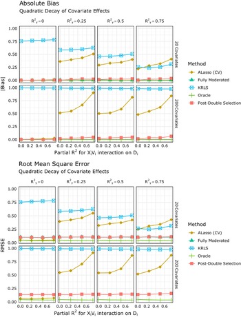
Figure 2 shows the results of these simulations. We omit the single-interaction model and the BART from these plots, because their outlier results obscure the relative performance of the other methods. We present the full results in Figure SM.1 in the Supplementary Material. With a low number of covariates (
 $K = 20$
), the fully moderated model dominates the feasible methods in terms of bias, across all settings. PDS is very close in performance, with slightly higher levels of bias, depending on the strength of the interactions. All of the other adaptive methods have large biases except for the adaptive lasso when the covariate–moderator interactions are unrelated to the outcome and so produce no omitted variables bias when they are omitted. KRLS has a large degree of bias that is relatively unaffected by the parameters varied here. BART (presented in the Supplementary Material) has similar bias to the adaptive lasso and KRLS but has significant RMSE driven by large variance in the estimator.
Simulation results. Notes: Bias (top) and root-mean-square error (bottom) of various methods when estimating interactions. Horizontal panels vary the partial
 $R^2$
of the
 $V_iX_i$
interactions on
 $Y_i$
, and vertical panels vary the number of covariates. The x-axis in each panel varies the partial
 $R^2$
of the
 $V_iX_i$
on
 $D_i$
.

In the high-dimensional setting (
 $K = 200$
), the fully moderated model is very numerically unstable, since the number of parameters (
 $403$
) is close to the sample size (
 $425$
), leading to RMSE that is too high to show on the graphs.Footnote
6
The results on the adaptive methods are remarkably similar here to in the low-dimensional setting, with slightly higher bias and RMSE for PDS. Here, KRLS almost always estimates a precise zero interaction, leading to near constant bias and RMSE across the parameter values.
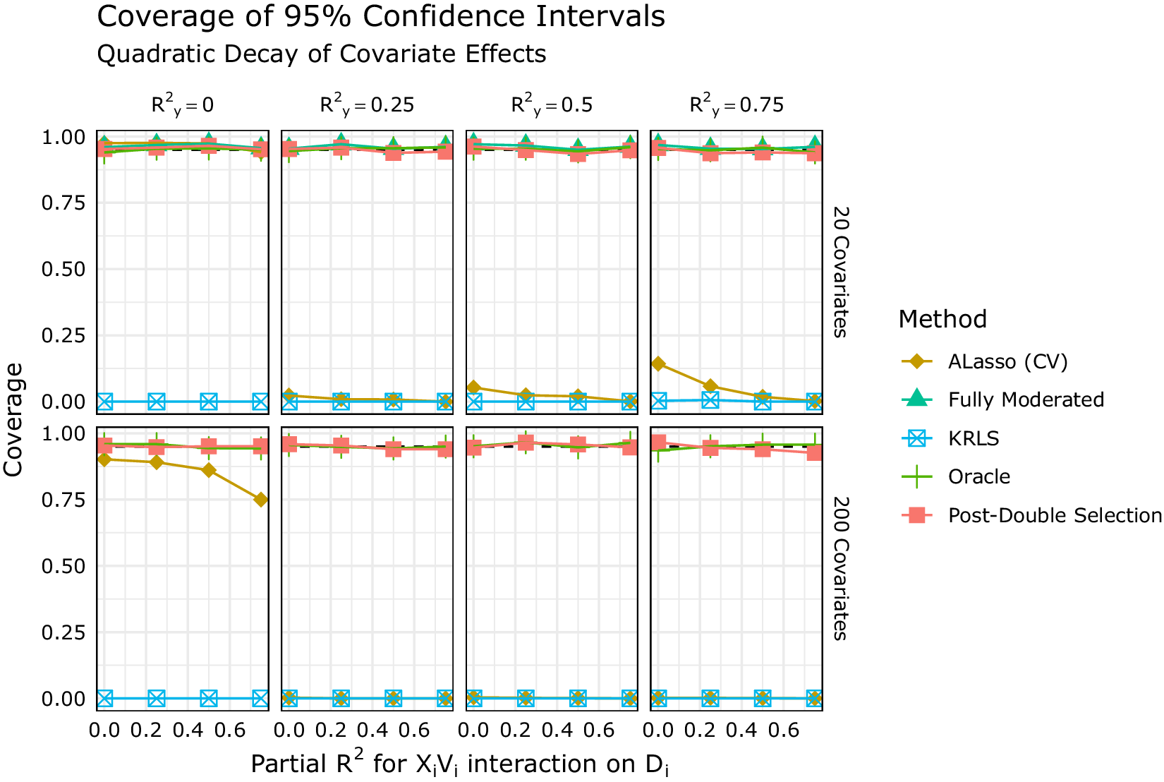
In Figure 3, we present the empirical coverage of nominal 95% confidence intervals from these estimators. With a small number of covariates, both the fully moderated and PDS approaches perform well, with PDS having coverage slightly closer to nominal levels except when the interactions are strongly related to the outcome, when it slightly undercovers. The residual bootstrap confidence intervals from the adaptive lasso undercover quite severely across a range of settings, mostly due to the bias of the method. With a high number of covariates, the PDS approach maintains its roughly nominal coverage, whereas the adaptive lasso shows an exaggerated pattern of its performance in the low-dimensional setting. In particular, the confidence intervals undercover even when the adaptive lasso has very little bias (that is, when
 $R^2_y = 0$
). Thus, in this quadratic decay setting, where the interactions are approximately sparse, the PDS estimator performs well in low- and high-dimensional settings, even when fully moderated models are infeasible. Furthermore, it appears to outperform several competing adaptive methods that have been applied to this problem in the past.
Simulation results for confidence interval coverage.
Note: Coverage rate of nominal 95% confidence intervals when estimating interactions.

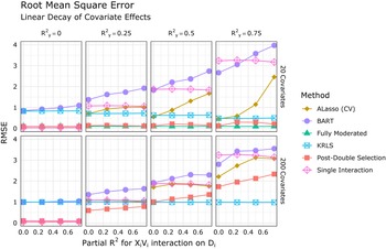
When can the lasso approaches to this problem fail? We investigate this with an alternative data-generating process where the covariate effects are more “dense.” In particular, we set the
 $\delta $
effects defined above to be functions of
 $j^{-1}$
instead of
 $j^{-2}$
, which spreads the same explanatory power over a larger set of covariates. We present the RMSE of the various estimators in Figure 4, where it is clear that the lasso-based estimators perform much worse than in the approximately sparse setting, especially in the high-dimensional setting. It is interesting to note, however, that PDS still outperforms the other adaptive methods except for KRLS in the high-dimensional setting, where its near-constant zero estimate of the interaction gives it the edge.
Simulation results under a dense coefficient setting. Notes: Root-mean-square error of various methods when estimating interactions. Horizontal panels vary the partial
 $R^2$
of the
 $V_iX_i$
interactions on
 $Y_i$
, and vertical panels vary the number of covariates. The x-axis in each panel varies the partial
 $R^2$
of the
 $V_iX_i$
on
 $D_i$
.

Overall, adaptive approaches are very suited to this task. As we show in the Supplementary Material, all of the adaptive methods investigated here can dramatically reduce bias over single-interaction methods except when the covariates are completely unrelated to the outcome. Furthermore, these methods can also improve efficiency (and estimability) over fully moderated models. The PDS approach appears to outperform the other adaptive approaches considered here in both bias and RMSE. We should note that the results for KRLS and BART are in some ways unfair to these methods, since they both focus on estimating the entire response surface rather than a particular interaction, like the lasso-based methods. While we focused on their off-the-shelf implementation, a worthwhile path for future research might be to estimate separate CEFs of the outcome within levels of
 $D_i$
and
 $V_i$
when both are binary. In the Supplementary Material, we also show that the PDS approach also outperforms a post-single selection approach unless interactions are unimportant for either the treatment or the outcome. Finally, the PDS approach appears to work best when the covariate interactions are either sparse or approximately sparse.
5 Empirical Illustrations
5.1 The Direct Primary and Third-Party Voting
The role of the direct primary in shaping American electoral politics has been of persistent interest to scholars. One argument surrounding this uniquely American institution is that, by creating a clear path to major party nominations by those other than party insiders (Hirano and Snyder Reference Hirano and Snyder2007), and by allowing for ideological heterogeneity within parties (Ansolabehere, Hirano, and Snyder Reference Ansolabehere, Hirano, Snyder, Brady and McCubbins2007), it reduced the electoral prominence of third parties. This argument is tested directly by Hirano and Snyder (Reference Hirano and Snyder2007) using a two-way fixed effects models to control for state-specific and year-specific unobserved confounders. In the South, the direct primary was a fundamentally different reform, tied up in the disfranchisement of African Americans and the consolidation of white Democratic one-party rule (Ware Reference Ware2002, pp. 18–20). With varying motivations for primary adoption across the North and the South, it is important to evaluate whether the effect of direct primary adoption is similar in the two regions. Hirano and Snyder (Reference Hirano and Snyder2007) do so by estimating separate models for the South and the non-South—in effect, a fully moderated model.
We focus on U.S. House elections, and take as our outcome variable the share of all U.S. House votes cast in a given state election for parties or individuals other than Democrats or Republicans.Footnote
7
 $^,$
Footnote
8
We measure direct primary adoption as an indicator variable for whether the direct primary was in widespread use in a given state and year.Footnote
9
Our moderator,
 $\textit {South}$
, is an indicator for whether a state is one of the 11 states of the former Confederacy. The single-interaction model can therefore be expressed as follows:
 $$ \begin{align} (100-\textit{DemShare}_{it}-\textit{RepShare}_{it}) &= \beta \left( \textit{Primary}_{it} \times \textit{South}_i \right) + \gamma\textit{Primary}_{it} + \alpha_i + \tau_t + \epsilon_{it}, \end{align} $$
where i indexes states and t indexes election years. The base term on
 $\textit {South}$
is absorbed by the state fixed effects
 $\alpha $
;
 $\tau $
is a year fixed effect. In this straightforward setup, the only interactions added in the fully moderated model are those between year fixed effects and the moderator.
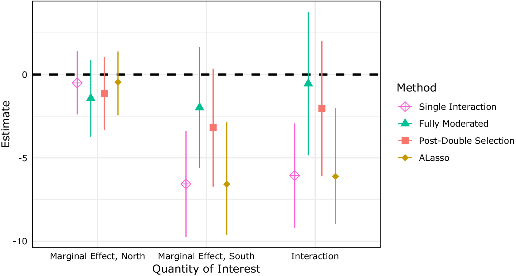
Figure 5 displays estimates from a single-interaction model given by Equation (11), a fully moderated model that adds interactions between the year fixed effects and the
 $\textit {South}$
indicator, our suggested PDS estimator, and the adaptive lasso, which is Beiser-McGrath and Beiser-McGrath’s (Reference Beiser-McGrath and Beiser-McGrath2020) suggested estimator. In Figure SM.9 in the Supplementary Material, we additionally report replication results using the post-single selection, KRLS, and BART estimators discussed above and in Beiser-McGrath and Beiser-McGrath (Reference Beiser-McGrath and Beiser-McGrath2020).
Effect of the direct primary in the American North and South. Notes: Estimates from the single-interaction, fully moderated, post-double selection (PDS), and adaptive lasso models described above. 95% confidence intervals are based on state-clustered standard errors (single-interaction, fully moderated, PDS) or state-blocked bootstrap (adaptive lasso).

The estimates from the single-interaction and adaptive lasso estimates are extremely similar, and are starkly different from the fully moderated and PDS results. While all four model types agree that there is a small, statistically insignificant effect of direct primary adoption in northern states, the single-interaction and adaptive lasso etimators indicate that the effect is significantly more negative, and indeed negative overall, in the South. The fully moderated model indicates no such interaction between region and primary adoption, with a near-zero estimate of the interaction and a small and insignificant marginal effect of direct primary adoption in the South. The conclusions of the PDS estimator lie in-between these extremes, with a marginally significant negative marginal effect of primary adoption in the South. This replication suggests key features of these different estimators. First, the adaptive lasso estimator here fails to select potentially impactful interactions that condition the relationship between primary adoption and region, leading to estimates that are extremely similar to the single-interaction model. Second, the PDS estimator appears to hedge against possible overfitting by the fully moderated model, although its conclusions remain largely consistent with it.
5.2 Regime Type and Remittances
The role of remittances in shaping political activity is an active area of research, with some literature suggesting that remittances can buttress authoritarian governments, and others suggesting that remittances can spur political change in democratizing or nondemocratic countries. Entering into this debate, Escribà-Folch, Meseguer, and Wright (Reference Escribà-Folch, Meseguer and Wright2018) explore the relationship between remittances and political protest, a first step on the path of democratization. They argue that remittances ought to be associated with greater levels of protest, but only in nondemocracies, and find evidence consistent with this claim.
To do so, the authors use novel (continuous) measures of remittances and protest and an array of control variables in a linear regression model with country and time fixed effects.Footnote
10
To test the heterogeneous effects of remittances across regime type,
 $\textit {Remit}$
is interacted with a binary indicator for regime type,
 $\textit {Autocracy}$
. This yields the following specification:
 $$ \begin{align} \textit{Protest}_{it} &= \beta \left( \textit{Remit}_{it} \times \textit{Autocracy}_{it}\right) + \gamma \textit{Remit}_{it} + \phi \textit{Autocracy}_{it} + \boldsymbol{\psi}' \textbf{X}_{it} + \alpha_i + \tau_t + \epsilon_{it}, \end{align} $$
where
 $\textbf {X}_{it}$
is a vector of time-varying controls. In keeping with the above discussion, however, we argue that this model makes important assumptions that can be easily relaxed. Specifically, we note that this model assumes that all covariates—including, importantly, the fixed effects—other than the main treatment of interest have the same (linear) effect in democracies and autocracies. To explore the sensitivity of inferences to modeling choices, we replicated the main specification of Escribà-Folch et al. (Reference Escribà-Folch, Meseguer and Wright2018, Table 1, column 2), using methods discussed above.
Figure 6 plots points estimates and confidence intervals from four of these approaches.Footnote 11 We report these estimates for three quantities of interest: the marginal effect of remittances in autocracies, the marginal effect of remittances in democracies, and the interaction between remittances and autocracy. As Figure 6 makes clear, estimates differ considerably depending on the estimator used.
Remittances, protest, and regime type. Notes: Estimates from the single-interaction, fully moderated, post-double selection (PDS), and adaptive lasso models described above. 95% confidence intervals are based on regime-clustered standard errors (single-interaction, fully moderated, PDS) or regime-blocked bootstrap (adaptive lasso).

All models are consistent in their conclusion that remittances are important predictors of protest in autocracies, but only the single-interaction model supports the authors’ original conclusion that remittances matter differently, to a statistically significant degree, in autocracies and democracies. For the single-interaction model, the estimated marginal effect in democracies is almost exactly zero; the interaction between remittances and autocracy is positive and significant. Among the other estimators, the adaptive lasso comes closest to affirming an interaction between regime type and remittances, although the estimate does not approach statistical significance. The fully moderated and PDS models, however, agree that there is little if any difference in the effect of remittances across regime type. Interestingly, these models disagree about the extent to which remittances matter at all; the fully moderated model suggests they matter substantially in both democracies and autocracies, while the PDS estimates are considerably lower for both regime types, and only statistically significant in autocracies. As expected, the use of the PDS estimator produces somewhat tighter confidence intervals than the fully moderated model.
6 Conclusion
In this paper, we review how model misspecification can affect the estimation of interactive effects in regression models. A single multiplicative interaction term can be biased when interactions between the same moderator and other covariates are omitted from the model (Beiser-McGrath and Beiser-McGrath Reference Beiser-McGrath and Beiser-McGrath2020). These omitted interactions can considerably change the estimated effect heterogeneity and lead scholars to draw misleading conclusions. To avoid this issue, we advocate for two possible solutions. The first is a fully moderated (or split-sample) model that includes an interaction between the moderator and all variables in the model. When this a fully moderated model is not possible due to sample size, we recommend a machine learning approach, but as we describe above, it is important to choose one that avoids the types of regularization bias common in those techniques. In particular, we proposed one solution, PDS, that utilizes the lasso for model selection, but not estimation, and applies it both the outcome and the main independent variable of interest.
Based on our analyses, we recommend that scholars think carefully about model misspecification when estimating interactions, and when possible, use more flexible estimation procedures for this purpose. This includes assessing linearity of the interaction, as Hainmueller et al. (Reference Hainmueller, Mummolo and Xu2019) emphasize, but also to consider how lower-order terms of the moderator and covariates, among other nuisances, affect inferences. In this paper, we have focused on the lasso, but other machine learning methods may also provide flexible ways of estimating interactions. When using other machine learning methods, though, it is important to assess how they perform in terms of estimating low-dimensional parameters, since many of these methods are designed for general prediction tasks and not the traditional inference of the applied social sciences.
Acknowledgments
Thanks to Stephen Chaudoin, Kosuke Imai, Josh Kertzer, Gary King, Horacio Larreguy, Christoph Mikulaschek, Pia Raffler, Maya Sen, Daniel Smith, Dustin Tingley, Yuhua Wang, Soichiro Yamauchi, and Xiang Zhou for helpful comments and discussions. All errors remain our own.
Data Availability Statement
Open-source software to implement the method of this paper are included in the inters R package. Data and code to replicate the results of this paper can be found in Blackwell and Olson (Reference Blackwell and Olson2021).
Supplementary Material
For supplementary material accompanying this paper, please visit https://doi.org/10.1017.pan.2021.19.