1 Introduction
Combustion noise plays a key role in the instability of many combustion systems (Strahle Reference Strahle1978; Docquier & Candel Reference Docquier and Candel2002; Lieuwen Reference Lieuwen2012; Dowling & Mahmoudi Reference Dowling and Mahmoudi2015; Ihme Reference Ihme2017). The noise generated by turbulent premixed flames deserves special attention since they are common in contemporary, low-emission gas turbines.
In one of the earlier studies of combustion noise, Smith & Kilham (Reference Smith and Kilham1963) experimentally investigated sound generation by open, turbulent, premixed flames. Like several later works, they observed that the radiated sound was predominantly monopolar, and they argued that the emitted sound originated from monopolar sources throughout the flame. In the same year, Bragg (Reference Bragg1963) proposed a theory to describe the relationship between the sound production and combustion by assuming that the generated noise was the result of changes in the flame volume, which was assumed to be directly proportional to changes in the rate of heat release rate. Many subsequent theoretical studies of sound generation by turbulent premixed flames have also attempted to relate the radiated sound to changes in the flame volume or the heat release rate e.g. Hurle et al. (Reference Hurle, Price, Sugden and Thomas1968), Strahle (Reference Strahle1978), Kotake & Takamoto (Reference Kotake and Takamoto1990), Dowling (Reference Dowling1992), Schuller, Durox & Candel (Reference Schuller, Durox and Candel2003), Candel, Durox & Schuller (Reference Candel, Durox and Schuller2004), Rajaram & Lieuwen (Reference Rajaram and Lieuwen2009), Swaminathan et al. (Reference Swaminathan, Balachandran, Xu and Dowling2011a ,Reference Swaminathan, Xu, Dowling and Balachandran b ), Liu (Reference Liu2015).
There are several numerical studies on sound generation by turbulent flames using large-eddy simulation (LES) e.g. Bui et al. (Reference Bui, Meinke, Schröder, Flemming, Sadiki and Janicka2005), Birbaud et al. (Reference Birbaud, Ducruix, Durox and Candel2006), Flemming, Sadiki & Janicka (Reference Flemming, Sadiki and Janicka2007), Bui, Schröder & Meinke (Reference Bui, Schröder and Meinke2008), Bui et al. (Reference Bui, Ihme, Schröder and Pitsch2009), Ihme, Pitsch & Bodony (Reference Ihme, Pitsch and Bodony2009), Ihme & Pitsch (Reference Ihme and Pitsch2012), Silva et al. (Reference Silva, Leyko, Nicoud and Moreau2013), Zhang et al. (Reference Zhang, Habisreuther, Bockhorn, Nawroth and Paschereit2013), Livebardon et al. (Reference Livebardon, Moreau, Poinsot and Bouty2015). Although the significance of the heat release rate fluctuations was confirmed by these studies, varying levels of agreement between LES and experiment was observed (Flemming et al. Reference Flemming, Sadiki and Janicka2007; Bui et al. Reference Bui, Ihme, Schröder and Pitsch2009) and several sources of uncertainty such as sub-grid modelling (Ihme et al. Reference Ihme, Pitsch and Bodony2009) and grid resolution (Ihme et al. Reference Ihme, Pitsch and Bodony2009; Silva et al. Reference Silva, Leyko, Nicoud and Moreau2013) were found. Nonetheless, LES appears to be the only plausible tool for examining sound generation in practical turbulent flames.
In contrast to LES, direct numerical simulation (DNS) should not suffer from problems associated with grid resolution or sub-grid modelling. However, DNS of sound generation by unconfined premixed flames is relatively rare (e.g. Miyauchi, Tanahashi & Li Reference Miyauchi, Tanahashi and Li2001; Zhao & Frankel Reference Zhao and Frankel2001; Tanahashi et al. Reference Tanahashi, Tsukinari, Saitoh, Miyauchi, Choi, Ikame, Kishi, Harumi and Hiraoka2002; Talei, Brear & Hawkes Reference Talei, Brear and Hawkes2012a ) because of the computational cost incurred by resolving both the flame and the radiated sound simultaneously, and the sensitivity of the acoustic field to numerical issues that are particularly challenging in combusting flows (Zhao & Frankel Reference Zhao and Frankel2001; Talei, Brear & Hawkes Reference Talei, Brear and Hawkes2014). As a result, all previous DNS studies appear to either feature a large one- or two-dimensional domain or a relatively small three-dimensional configuration (Miyauchi et al. Reference Miyauchi, Tanahashi and Li2001; Tanahashi et al. Reference Tanahashi, Tsukinari, Saitoh, Miyauchi, Choi, Ikame, Kishi, Harumi and Hiraoka2002). Once again, a common feature of these studies were the importance of heat release rate fluctuations as a source of noise.
Flame annihilation is one mechanism that can lead to large fluctuations of the heat release rate in premixed flames (Kidin et al. Reference Kidin, Librovich, MacQuisten, Roberts and Vuillermoz1988; Schuller et al. Reference Schuller, Durox and Candel2003; Candel et al. Reference Candel, Durox and Schuller2004; Talei, Brear & Hawkes Reference Talei, Brear and Hawkes2011; Brear et al. Reference Brear, Nicoud, Talei, Giauque and Hawkes2012; Talei et al. Reference Talei, Brear and Hawkes2012a ; Talei, Hawkes & Brear Reference Talei, Hawkes and Brear2012b ; Talei et al. Reference Talei, Brear and Hawkes2014; Jiménez et al. Reference Jiménez, Haghiri, Talei, Brear and Hawkes2015). During annihilation, flame surfaces collide with each other, leading to rapid consumption of the unburned gas trapped between the flame surfaces, and can therefore produce noise. In a number of theoretical and numerical studies of laminar flame annihilation, Talei et al. (Reference Talei, Brear and Hawkes2011, Reference Talei, Brear and Hawkes2012a ,Reference Talei, Hawkes and Brear b , Reference Talei, Brear and Hawkes2014) investigated the impact of key flame parameters such as flame thickness, flame speed, Zel’dovich number, temperature ratio and Lewis number on flame annihilation and the produced sound. However, the significance of annihilation events in noise generation by turbulent premixed flames appears to have received no examination, even though they have been observed in numerous non-acoustic studies of turbulent, premixed flames (e.g. Echekki, Chen & Gran Reference Echekki, Chen and Gran1996; Balachandran et al. Reference Balachandran, Ayoola, Kaminski, Dowling and Mastorakos2005; Griffiths et al. Reference Griffiths, Chen, Kolla, Cant and Kollmann2015).
The aim of this paper is therefore twofold. First, we present three-dimensional DNS of sound generation by open turbulent premixed flames. Two turbulent, methane–air flames are studied with equivalence ratios
 $\unicode[STIX]{x1D719}=0.7$
and 1.0. Second, the significance of annihilation events will be examined using a simple model that is based on one of our previous studies (Talei et al.
Reference Talei, Brear and Hawkes2012a
).
2 Governing equations
The governing equations for the conservation of mass, momentum, total energy and reactant species mass fraction are solved using a single-step, irreversible chemical reaction. The non-dimensionalised forms of the equations of motion are obtained using the flow premixture quantities, where the superscript ‘*’ represents dimensional values and the subscript
 $ref$
corresponds to the values of the reactant at the inlet boundary:
 $$\begin{eqnarray}\displaystyle \left.\begin{array}{@{}l@{}}\boldsymbol{x}_{j}=\displaystyle \frac{\boldsymbol{x}_{j}^{\ast }}{D},\quad t=\frac{t^{\ast }\,c_{ref}}{D},\quad \boldsymbol{u}_{j}=\frac{\boldsymbol{u}_{j}^{\ast }}{c_{ref}},\quad \unicode[STIX]{x1D70C}=\frac{\unicode[STIX]{x1D70C}^{\ast }}{\unicode[STIX]{x1D70C}_{ref}},\quad T=\frac{T^{\ast }}{(\unicode[STIX]{x1D6FE}-1)T_{ref}},\\[12.0pt] Y_{R}=\displaystyle \frac{Y_{R}^{\ast }}{Y_{R,\,ref}},\quad p=\frac{p^{\ast }}{\unicode[STIX]{x1D70C}_{ref}c_{ref}^{2}}\quad \text{and}\quad \unicode[STIX]{x1D707}=\frac{\unicode[STIX]{x1D707}^{\ast }}{\unicode[STIX]{x1D707}_{ref}}.\end{array}\right\} & & \displaystyle\end{eqnarray}$$
In the above,
 $\boldsymbol{x}$
and
 $t$
are the spatial coordinate vector and time, respectively. In addition,
 $c$
is the sonic velocity,
 $\boldsymbol{u}_{j}$
is the
 $j$
-component of velocity vector,
 $\unicode[STIX]{x1D70C}$
is the mixture density,
 $T$
is the temperature,
 $\unicode[STIX]{x1D6FE}$
is the heat capacity ratio and considered to be 1.4,
 $Y_{R}$
is the reactant mass fraction (progress variable),
 $p$
is the pressure,
 $D$
is the jet diameter and
 $\unicode[STIX]{x1D707}$
is the dynamic viscosity where its variation with temperature is modelled as
 $=(T/T_{ref})^{0.76}$
(Poinsot, Echekki & Mungal Reference Poinsot, Echekki and Mungal1992). The following non-dimensional parameters are also defined:
 $$\begin{eqnarray}\displaystyle \left.\begin{array}{@{}l@{}}\mathit{Re}=\displaystyle \left(\frac{c\,D}{\unicode[STIX]{x1D708}}\right)_{ref},\quad \mathit{Pr}=\left(\frac{\unicode[STIX]{x1D708}}{D_{th}}\right)_{ref},\quad \mathit{Le}=\left(\frac{D_{th}}{D_{m}}\right)_{ref}=1,\\[13.0pt] \mathit{Da}=\displaystyle \left(\frac{\unicode[STIX]{x1D6EC}\,D}{c}\right)_{ref}\quad \text{and}\quad \mathit{Sc}=\mathit{Le}~\mathit{Pr},\end{array}\right\} & & \displaystyle\end{eqnarray}$$
where Re is the acoustic Reynolds number, Pr is the Prandtl number, Sc is the Schmidt number, Le is the Lewis number, Da is the Damköhler number,
 $D_{th}$
is the thermal diffusivity coefficient,
 $D_{m}$
is the binary mass diffusion coefficient,
 $\unicode[STIX]{x1D6EC}$
is the pre-exponential factor in the Arrhenius law and
 $\unicode[STIX]{x1D708}$
is the kinematic viscosity.
Using these parameters, the non-dimensional form of the governing equations may be expressed as
 $$\begin{eqnarray}\displaystyle & \displaystyle \frac{\unicode[STIX]{x2202}\unicode[STIX]{x1D70C}}{\unicode[STIX]{x2202}t}+\frac{\unicode[STIX]{x2202}\unicode[STIX]{x1D70C}\boldsymbol{u}_{i}}{\unicode[STIX]{x2202}\boldsymbol{x}_{i}}=0, & \displaystyle\end{eqnarray}$$
 $$\begin{eqnarray}\displaystyle & \displaystyle \frac{\unicode[STIX]{x2202}\unicode[STIX]{x1D70C}\boldsymbol{u}_{j}}{\unicode[STIX]{x2202}t}+\frac{\unicode[STIX]{x2202}\unicode[STIX]{x1D70C}\boldsymbol{u}_{i}\boldsymbol{u}_{j}}{\unicode[STIX]{x2202}\boldsymbol{x}_{i}}=-\frac{\unicode[STIX]{x2202}p}{\unicode[STIX]{x2202}\boldsymbol{x}_{j}}+\frac{\unicode[STIX]{x2202}\unicode[STIX]{x1D70F}_{ij}}{\unicode[STIX]{x2202}\boldsymbol{x}_{i}}, & \displaystyle\end{eqnarray}$$
 $$\begin{eqnarray}\displaystyle & \displaystyle \frac{\unicode[STIX]{x2202}\unicode[STIX]{x1D70C}E_{t}}{\unicode[STIX]{x2202}t}+\frac{\unicode[STIX]{x2202}\boldsymbol{u}_{j}(\unicode[STIX]{x1D70C}E_{t}+p)}{\unicode[STIX]{x2202}\boldsymbol{x}_{j}}=\frac{\unicode[STIX]{x2202}\boldsymbol{u}_{i}\unicode[STIX]{x1D70F}_{ij}}{\unicode[STIX]{x2202}\boldsymbol{x}_{j}}-\frac{\unicode[STIX]{x2202}\boldsymbol{q}_{j}}{\unicode[STIX]{x2202}\boldsymbol{x}_{j}}, & \displaystyle\end{eqnarray}$$
and
 $$\begin{eqnarray}\displaystyle & \displaystyle \frac{\unicode[STIX]{x2202}\unicode[STIX]{x1D70C}Y_{R}}{\unicode[STIX]{x2202}t}+\frac{\unicode[STIX]{x2202}\unicode[STIX]{x1D70C}\boldsymbol{u}_{j}Y_{R}}{\unicode[STIX]{x2202}\boldsymbol{x}_{j}}=\frac{\unicode[STIX]{x2202}}{\unicode[STIX]{x2202}\boldsymbol{x}_{j}}\left(\frac{1}{Re\mathit{Sc}}\unicode[STIX]{x1D707}\frac{\unicode[STIX]{x2202}Y_{R}}{\unicode[STIX]{x2202}\boldsymbol{x}_{j}}\right)+\dot{\unicode[STIX]{x1D714}}_{R}, & \displaystyle\end{eqnarray}$$
where
 $$\begin{eqnarray}\displaystyle & \displaystyle p=\frac{\unicode[STIX]{x1D6FE}-1}{\unicode[STIX]{x1D6FE}}\unicode[STIX]{x1D70C}T, & \displaystyle\end{eqnarray}$$
 $$\begin{eqnarray}\displaystyle & \displaystyle E_{t}=\frac{T}{\unicode[STIX]{x1D6FE}}+\frac{1}{2}\boldsymbol{u}_{i}\boldsymbol{u}_{i}+\frac{\unicode[STIX]{x1D70F}}{\unicode[STIX]{x1D6FE}-1}Y_{R}, & \displaystyle\end{eqnarray}$$
 $$\begin{eqnarray}\displaystyle & \displaystyle \unicode[STIX]{x1D70F}_{ij}=\frac{\unicode[STIX]{x1D707}}{\mathit{Re}}\left[\frac{\unicode[STIX]{x2202}\boldsymbol{u}_{i}}{\unicode[STIX]{x2202}\boldsymbol{x}_{j}}+\frac{\unicode[STIX]{x2202}\boldsymbol{u}_{j}}{\unicode[STIX]{x2202}\boldsymbol{x}_{i}}-\frac{2}{3}\frac{\unicode[STIX]{x2202}\boldsymbol{u}_{k}}{\unicode[STIX]{x2202}\boldsymbol{x}_{k}}\unicode[STIX]{x1D6FF}_{ij}\right], & \displaystyle\end{eqnarray}$$
 $$\begin{eqnarray}\displaystyle & \displaystyle \boldsymbol{q}_{j}=-\frac{\unicode[STIX]{x1D707}}{\mathit{Re }~\mathit{ Pr}}\frac{\unicode[STIX]{x2202}T}{\unicode[STIX]{x2202}\boldsymbol{x}_{j}}-\frac{\unicode[STIX]{x1D707}}{\mathit{Re }~\mathit{ Sc}}\frac{\unicode[STIX]{x1D70F}}{(\unicode[STIX]{x1D6FE}-1)}\frac{\unicode[STIX]{x2202}Y_{R}}{\unicode[STIX]{x2202}\boldsymbol{x}_{j}}, & \displaystyle\end{eqnarray}$$
and
 $$\begin{eqnarray}\displaystyle & \displaystyle \dot{\unicode[STIX]{x1D714}}_{R}=-\mathit{Da}\unicode[STIX]{x1D70C}Y_{R}~\exp \left[-\frac{\unicode[STIX]{x1D6FD}\,(1-\unicode[STIX]{x1D703})}{1-\unicode[STIX]{x1D6FC}\,(1-\unicode[STIX]{x1D703})}\right], & \displaystyle\end{eqnarray}$$
with
 $$\begin{eqnarray}\displaystyle & \displaystyle \unicode[STIX]{x1D70F}=\unicode[STIX]{x1D6FC}/(1-\unicode[STIX]{x1D6FC}),\quad \text{and}\quad \unicode[STIX]{x1D703}=\frac{(\unicode[STIX]{x1D6FE}-1)T-1}{\unicode[STIX]{x1D70F}}. & \displaystyle\end{eqnarray}$$
Note that
 $E_{t}$
is the total energy (including sensible, kinetic and chemical energy),
 $\boldsymbol{q}_{j}$
is the heat flux vector,
 $\unicode[STIX]{x1D70F}_{ij}$
is the
 $ij$
-component of the viscous stress tensor,
 $\unicode[STIX]{x1D6FF}_{ij}$
is the Kronecker delta and
 $\dot{\unicode[STIX]{x1D714}}_{R}$
is the reactant species reaction rate. In addition,
 $\unicode[STIX]{x1D6FC}$
is the heat release parameter and
 $\unicode[STIX]{x1D6FD}$
is the Zel’dovich number:
 $$\begin{eqnarray}\displaystyle & \displaystyle \unicode[STIX]{x1D6FC}=\frac{T_{f}-T_{u}}{T_{f}}\quad \text{and}\quad \unicode[STIX]{x1D6FD}=\frac{E_{a}(T_{f}-T_{u})}{R\,T_{f}^{2}}. & \displaystyle\end{eqnarray}$$
Here,
 $T_{f}$
is the adiabatic flame temperature,
 $T_{u}$
is the fresh (unburned) mixture temperature,
 $E_{a}$
is the activation energy and
 $R$
is the gas constant.
3 Flow configuration and numerical set-up
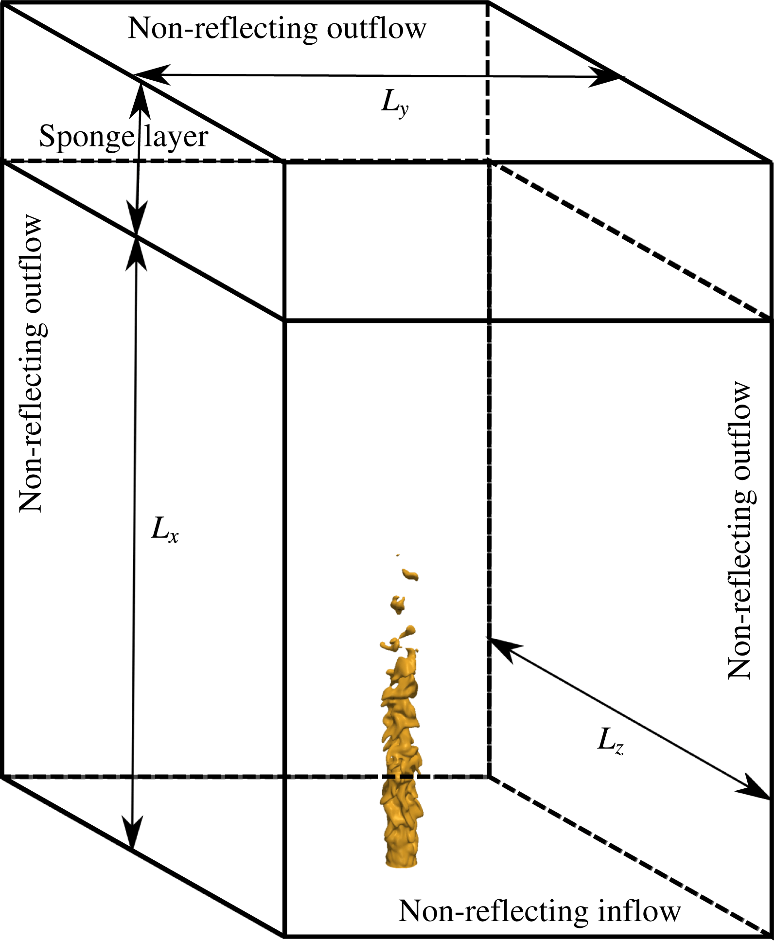
As shown in figure 1, a subsonic round jet of premixed reactant is injected into an open environment of combustion products at the adiabatic flame temperature. Methane/air combustion is considered at two different equivalence ratios (
 $\unicode[STIX]{x1D719}=0.7$
and 1.0), with the reactants preheated to
 $T_{u}=800~\text{K}$
at 1 atm. The reactant temperature is representative of modern gas turbines. A coflow with a low velocity magnitude (1 % of the jet mean velocity) surrounds the jet flame at the inflow at the product temperature.
A simple chemistry model is used to reduce the computational cost, since the resolution required for the study of sound generation by turbulent, premixed flames is significantly higher than for non-acoustic studies of combustion (Talei et al. Reference Talei, Brear and Hawkes2014). Whilst single-step chemistry is not always adequate to describe the flame structure, it can nonetheless be used to match several important parameters such as the laminar flame speed, the flame thickness, the temperature ratio and the Lewis number. The use of simple chemistry is therefore a logical first step in such studies, and is reasonably common in the literature (e.g. Haworth & Poinsot Reference Haworth and Poinsot1992; Poinsot et al. Reference Poinsot, Echekki and Mungal1992; Chakraborty & Cant Reference Chakraborty and Cant2009; Dunstan et al. Reference Dunstan, Swaminathan, Bray and Kingsbury2013; Karami et al. Reference Karami, Hawkes, Talei and Chen2015; Chakraborty, Konstantinou & Lipatnikov Reference Chakraborty, Konstantinou and Lipatnikov2016).
To construct the single-step chemical model, the required laminar flame speed, laminar flame thickness and adiabatic flame temperature were first obtained from PREMIX (Kee et al.
Reference Kee, Grcar, Smooke, Miller and Meeks1985) computations with detailed chemistry using GRI-MECH 3.0 (Smith et al.
Reference Smith, Golden, Frenklach, Moriarty, Eiteneer, Goldenberg, Bowman, Hanson, Song and Gardiner1999). The Zel’dovich number was also calculated following the procedure proposed by Law & Sung (Reference Law and Sung2000). The values of
 $Da_{ref}$
and
 $Re_{ref}$
were then determined such that the values of
 $S_{L}$
and
 $\unicode[STIX]{x1D6FF}_{th}$
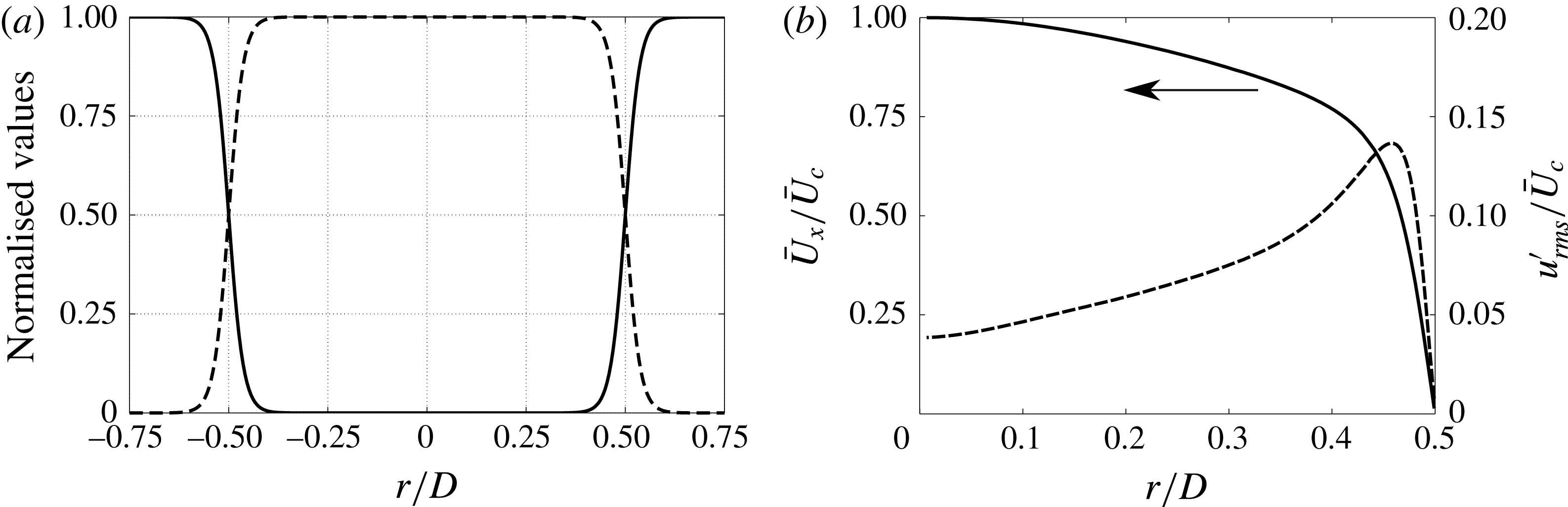
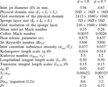
calculated from a laminar, unstrained premixed flame simulation with simple chemistry were matched to those calculated from a PREMIX computation for each case. The computational and flame parameters are summarised in table 1. The temperature and reactant species mass fraction profiles at the inlet boundary (see figure 2
a) were obtained using an unstrained laminar flame solution computed with the flame parameters, presented in table 1.
Schematic of the computational domain (not to scale). Note that the coordinate origin is located at the jet centreline on the inflow plane.

The mean and the root mean square (r.m.s.) profiles of the inlet streamwise velocity (see figure 2
b) were adapted from the DNS study of Wu & Moin (Reference Wu and Moin2008) for a fully developed turbulent pipe flow at
 $\mathit{Re}_{\mathit{D}}=5300$
. It should be noted that the choice of Reynolds number and
 $\unicode[STIX]{x1D6FF}_{th}/D$
were constrained by the computational cost. There is a difference in the inlet Mach numbers in order to keep the Reynolds number and the normalised laminar flame thickness (
 $\unicode[STIX]{x1D6FF}_{th}/D=0.07$
) the same for both values of
 $\unicode[STIX]{x1D719}$
, as can be seen in table 1.
To impose the velocity fluctuations at the inlet, a homogeneous isotropic turbulence field based on a prescribed turbulent energy spectrum (Passot & Pouquet Reference Passot and Pouquet1987) with a turbulence intensity of 3.7 % is first produced. (This value is equal to the turbulent intensity of the pipe flow simulation at the centreline, reported by Wu & Moin (Reference Wu and Moin2008).) The obtained velocity fluctuations were then rescaled using the turbulent intensity profile from Wu & Moin (Reference Wu and Moin2008), shown in figure 2(b). The resulting frozen velocity field was then added to the mean inlet velocity using Taylor’s hypothesis.
The domain was resolved by a three-dimensional, structured, Cartesian mesh. A uniform grid was used in the streamwise direction. An algebraically stretched mesh with an increasing grid spacing (
 $(\unicode[STIX]{x1D6E5}_{i+1}/\unicode[STIX]{x1D6E5}_{i})-1$
) not exceeding 2 % was used for
 $|y,z|>1.5D$
. The resulting mesh provides a uniform grid spacing with 200 grid points per jet diameter over a region covering one
 $D$
on each side of the jet. This ensures that the instantaneous flame brush always remains within this finely resolved region, with 14 grid points per laminar flame thickness. Extensive mesh-independence studies were performed to ensure that the internal structure of the flame was adequately resolved and the radiated sound was free of numerical noise.
(a) Normalised temperature
 $\unicode[STIX]{x1D703}$
(solid) and reactant species mass fraction
 $Y_{R}$
(dashed) profiles at the inlet boundary; (b) the mean inlet streamwise velocity (
 $\bar{U}_{x}/\bar{U}_{c}$
) profile (solid) and the normalised r.m.s. of streamwise velocity fluctuations
 $u_{rms}^{\prime }/\bar{U}_{c}$
(dashed) at the inlet boundary.

DNS parameters.

The governing equations (2.3) to (2.6) were solved using a modified version of the numerical solver S3D (Chen et al. Reference Chen, Choudhary, De Supinski, DeVries, Hawkes, Klasky, Liao, Ma, Mellor-Crummey and Podhorszki2009) known as S3D-SC (Karami et al. Reference Karami, Hawkes, Talei and Chen2015, Reference Karami, Hawkes, Talei and Chen2016, Reference Karami, Talei, Hawkes and Chen2017). This solver features an eighth-order central differencing scheme for spatial derivatives, combined with a six-stage, fourth-order explicit Runge–Kutta time integrator. In order to suppress the spurious short waves produced by the central finite differencing scheme, a tenth-order filter is applied (Kennedy, Carpenter & Lewis Reference Kennedy, Carpenter and Lewis2000) at every time step.
All inflow/outflow boundaries were carefully treated to avoid spurious noise reflections. So-called standard ‘Navier–Stokes characteristic boundary conditions (NSCBC)’ (Poinsot & Veynante Reference Poinsot and Veynante2005) were used at the outflow planes in the transverse directions. At the inflow boundary and the streamwise outflow plane the modified NSCBC known as ‘3DNSCBC’ (Yoo & Im Reference Yoo and Im2007) were used, accounting for the effect of transverse terms. A sponge layer (Colonius, Lele & Moin Reference Colonius, Lele and Moin1997; Bogey, Bailly & Juvé Reference Bogey, Bailly and Juvé2000) was used for each case in the streamwise direction from
 $20D$
to
 $25D$
to gradually damp the velocity fluctuation at the outflow boundary. The sponge layer parameters were carefully chosen to ensure a negligible effect on the upstream flow field (Bogey et al.
Reference Bogey, Bailly and Juvé2000).
The simulations were performed using a constant time step for 6 jet flow-through times
 $\unicode[STIX]{x1D70F}_{j}=L_{x}/U_{j}$
, and only the data from the last
 $4\unicode[STIX]{x1D70F}_{j}$
were used for post-processing. The computational costs for the stoichiometric and lean cases were 1.4 and 1.9 million CPU hours respectively running on 9216 computing cores (Intel Xeon E5-2690V3 ‘Haswell’ processors, 2.6 GHz).
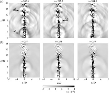
Instantaneous snapshots of the dimensionless dilatation field
 $\unicode[STIX]{x1D735}\boldsymbol{\cdot }\boldsymbol{u}$
on the central plane through the jet for (a)
 $\unicode[STIX]{x1D719}=1$
and (b)
 $\unicode[STIX]{x1D719}=0.7$
.

4 Discussion of DNS results
4.1 Noise sources
Instantaneous snapshots of the dimensionless dilatation field on the central
 $x$
–
 $y$
plane through the jet are shown for both equivalence ratios in figure 3. (It can be readily shown that the dilatation
 $\unicode[STIX]{x1D735}\boldsymbol{\cdot }\boldsymbol{u}$
and the pressure are related in the far field (Colonius et al.
Reference Colonius, Lele and Moin1997).) The reader is also referred to an animation of the dilatation field for these two cases in the supplementary material available at https://doi.org/10.1017/jfm.2018.115. The acoustic fields for both cases clearly feature monopolar sound sources originating from the flame. Weaker monopolar sources appear in the lean flame. Since both cases have the same Reynolds number and inlet turbulence intensities, this observation is likely related to a difference in chemical parameters between the two cases.
Instantaneous iso-surface with
 $Y_{R}=0.122$
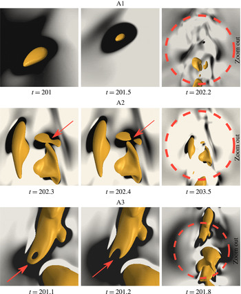
superimposed on the dilatation field for the three labelled events A1, A2 and A3 observed in figure 3. The dashed circle shows the monopolar sound wave generated by each annihilation event.

Figure 4 shows a flame iso-surface for events A1, A2 and A3 in figure 3 superimposed on the dilatation field. An iso-surface with
 $Y_{R}=0.122$
for
 $\unicode[STIX]{x1D719}=1.0$
is considered. This iso-surface is selected because it is close to the point of peak heat release in a one-dimensional premixed flame with the same chemistry. The event A1 involves consumption of a pocket of unburned gases in the downstream region near the flame tip. Consistent with our earlier works (Talei et al.
Reference Talei, Hawkes and Brear2012b
, Reference Talei, Brear and Hawkes2014), we refer to this phenomenon as ‘flame island burn out’. Event A2 is referred to as a ‘flame pinch off’, with a pocket of unburned gases locally detaching from the flame surface. Finally, the event A3 takes place when flame-to-flame interaction first results in the formation of a tunnel of burned gas, and then the local flame area is lost due to cusp retraction associated with another pinch-off event. We call this first event ‘tunnel formation’. All these identified events can be classified as upstream interactions since a portion of the unburned gas is consumed by propagation of flame surfaces (Chen & Sohrab Reference Chen and Sohrab1995). The topology of these events has been studied by Dunstan et al. (Reference Dunstan, Swaminathan, Bray and Kingsbury2013) and more recently by Griffiths et al. (Reference Griffiths, Chen, Kolla, Cant and Kollmann2015). Figure 3 suggests that these frequent flame annihilation events play an important role in the generation of sound.
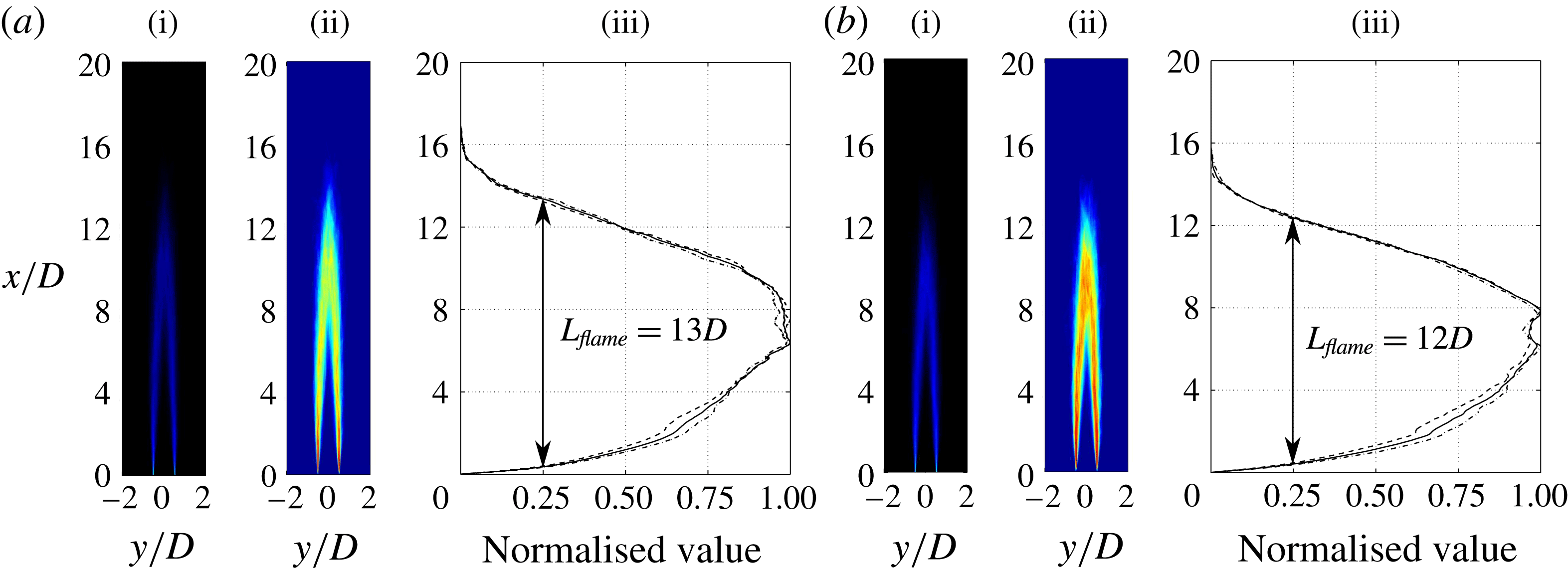
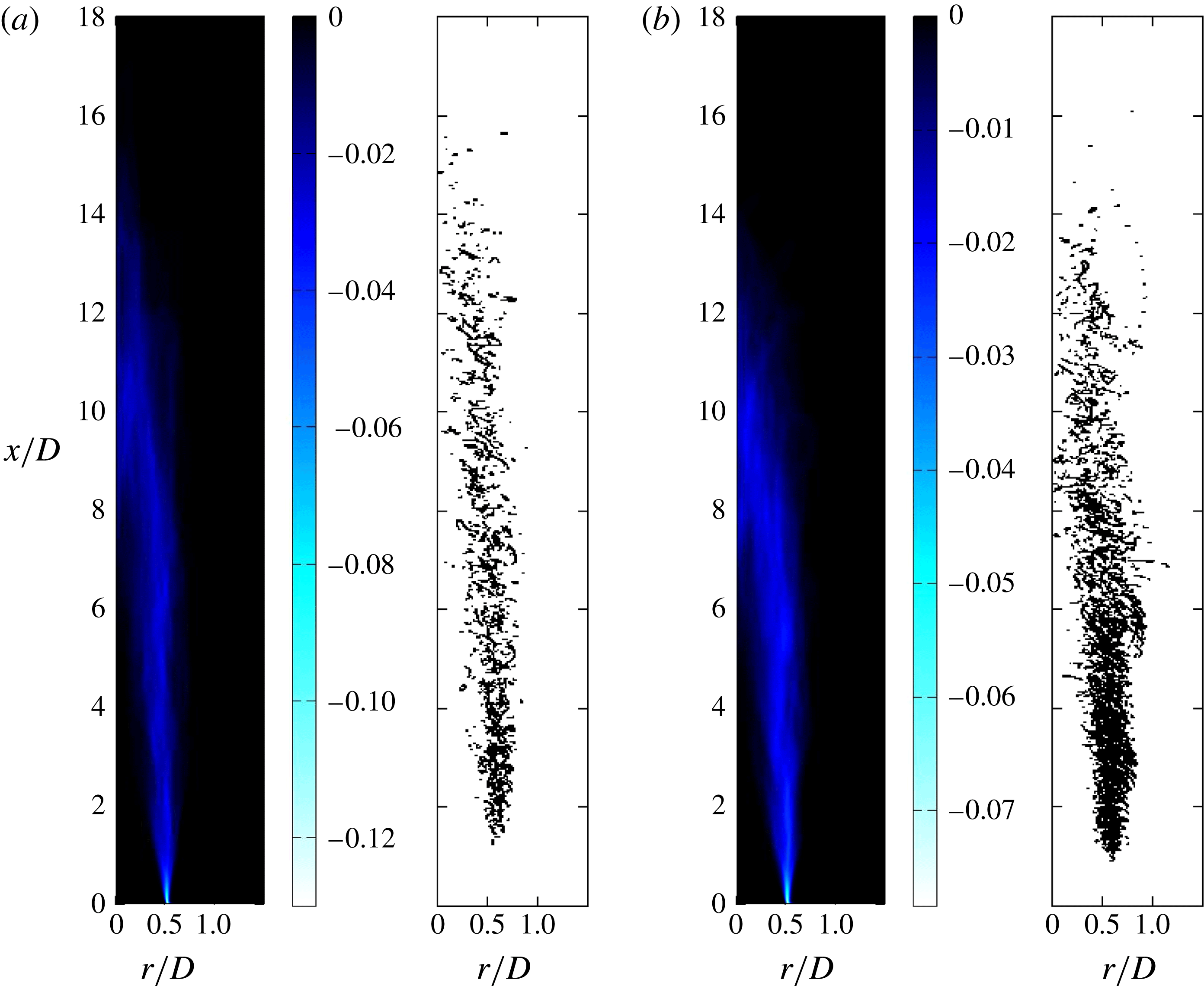
(i) Time-averaged reaction rate; (ii) variance of reaction rate; (iii) horizontally integrated variance field normalised by its maximum value (dashed:
 $x{-}y$
plane, dash-dot:
 $x{-}z$
plane and solid: the average of these planes) for (a)
 $\unicode[STIX]{x1D719}=1.0$
and (b)
 $\unicode[STIX]{x1D719}=0.7$
.

4.2 Spectral analysis
Rajaram & Lieuwen (Reference Rajaram and Lieuwen2009) showed that a peak Strouhal number
 $St_{peak}=f_{peak}L_{flame}/U_{av}$
of the far-field spectrum was always of order unity and varied between 0.5 and 2.2 across a large set of turbulent premixed flames tested, where
 $L_{flame}$
was a flame length and
 $U_{av}$
was the cold flow, bulk jet velocity. It should, however, be noted that Rajaram & Lieuwen (Reference Rajaram and Lieuwen2009) calculated their flame length using the variance in the intensity of chemiluminescence emitted by the flame at a given point in space. The flame length (
 $L_{flame}$
) was then defined as the distance between the heights where the horizontally integrated intensity of the variance image crosses a quarter of its maximum value. In the present study, the flame length was therefore calculated using the variance of the reaction rate field. As depicted in figure 5, these flame lengths were approximately equal to
 $13D$
and
 $12D$
for the stoichiometric and lean cases, respectively. The spectrum of the produced sound is calculated on a plane perpendicular to the jet axis at
 $x=10D$
using thirty two virtual microphones that were uniformly distributed at
 $r=6D$
. To reduce the so-called ‘spectral leakage’, a modified Hanning window (Lockard Reference Lockard2000) with 50 % overlap (Bui et al.
Reference Bui, Schröder and Meinke2008) was used to perform the fast Fourier transform (FFT) at each probe. The data for
 $\unicode[STIX]{x1D719}=1$
and 0.7 cases were collected for 1.43 and 2.9 ms. Since we have used a Hanning window with 50 % overlap, the lowest frequency that we can capture from the DNS is then approximately 1 kHz. This computational study is already very resource intensive, it is therefore impractical to reduce this lower frequency bound significantly, as this requires a corresponding increase in the computational cost.
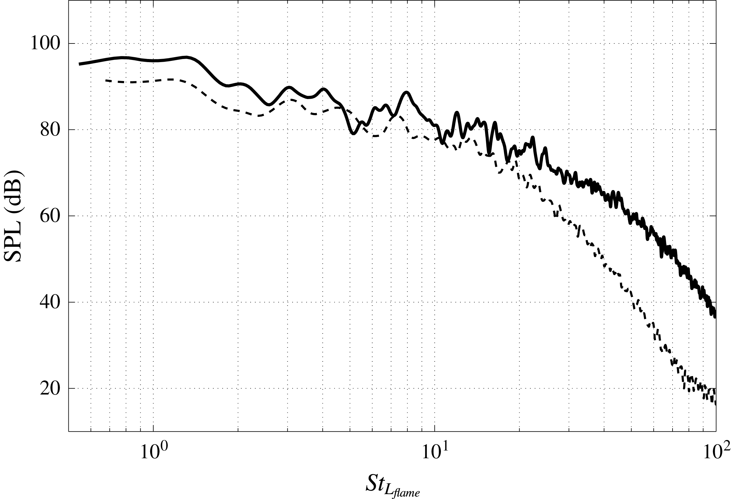
The averaged spectrum for both cases is shown in figure 6. The magnitude of the noise radiated by the stoichiometric flame is greater than that of the lean flame. This is examined later in this section. Using the calculated flame lengths, the peak Strouhal numbers for the stoichiometric and lean flames are 1.3 and 1.2, respectively, which fall within the range found experimentally by Rajaram & Lieuwen (Reference Rajaram and Lieuwen2009).
However, Rajaram & Lieuwen (Reference Rajaram and Lieuwen2009) also observed that the high frequency spectra rolls off at 42–64 (dB/decade) across
 $St_{L_{flame}}\sim 1{-}100$
for several different flames with
 $Re_{D}>10^{4}$
. This is not observed in the present study. There are several potential reasons for this observed difference. Those expected to be of particular significance are the two studies’ differing inflow turbulence, differing forms of flame stabilisation, and the present study’s lower jet Reynolds number of
 $\mathit{Re}_{D}\sim 5000$
.
Noise spectrum for
 $\unicode[STIX]{x1D719}=1.0$
(solid) and
 $\unicode[STIX]{x1D719}=0.7$
(dashed) considering 32 equally spaced probes at
 $x/D=10$
and
 $r/D=6$
. The horizontal axis shows Strouhal number based on flame length (
 $St_{L_{flame}}=fL_{flame}/U_{av}$
). The vertical axis shows the sound pressure level (SPL) in dB.

It is also worth mentioning that our DNS is undertaken at significantly different conditions to experimental studies such as Rajaram & Lieuwen (Reference Rajaram and Lieuwen2009). The same range of frequencies for DNS and experiment should therefore not be expected. Nonetheless, our captured range of frequencies non-dimensionalised by the frequency of peak emission is approximately between 0.4 and 100, which is in agreement with the range observed by Rajaram & Lieuwen (Reference Rajaram and Lieuwen2009) for natural gas (the relevant fuel to our study).
To shed light on the reason for the stoichiometric flame being louder than the lean flame, the scaling analysis performed by Rajaram, Gray & Lieuwen (Reference Rajaram, Gray and Lieuwen2006) is extended here. In this scaling, the total acoustic power,
 $P$
, is considered to be proportional to
 $(\text{d}Q/\text{d}t)^{2}$
. The underlying assumption is the heat release rate fluctuations,
 $\text{d}Q/\text{d}t$
, being the dominant source of noise, as discussed in § 1. The following scaling can then be derived:
 $$\begin{eqnarray}\displaystyle & \displaystyle \frac{\text{d}Q}{\text{d}t}\sim {\displaystyle \frac{Q_{char}}{t_{char}}}, & \displaystyle\end{eqnarray}$$
where
 $Q_{char}$
is the characteristic heat release rate estimated by
 ${\dot{m}}c_{p}(T_{b}-T_{u})$
and
 $t_{char}$
is the characteristic time scale estimated by
 $1/f_{peak}$
. Rajaram & Lieuwen (Reference Rajaram and Lieuwen2009) showed that the frequency of peak emission can be scaled with
 $U/L_{flame}$
. This is analogous to the scaling performed for non-reacting jets, in which the relevant frequency for sound generation is estimated as
 $U/D$
(Dowling & Ffowcs Williams Reference Dowling and Ffowcs Williams1983). Considering a premixed flame as a monopolar source of noise, it is reasonable to assume that the relevant length scale is the averaged flame length. These assumptions then lead to:
 $$\begin{eqnarray}\displaystyle & \displaystyle \frac{\text{d}Q}{\text{d}t}\sim \unicode[STIX]{x1D70C}_{u}UD^{2}c_{p}(T_{b}-T_{u})f_{peak}\sim \unicode[STIX]{x1D70C}_{u}c_{p}(T_{b}-T_{u})U^{2}D^{2}/L_{flame}. & \displaystyle\end{eqnarray}$$
The averaged flame length can be then estimated by assuming a small flame cone angle using the following expressions:
 $$\begin{eqnarray}\displaystyle & \displaystyle L_{flame}\sim UD/S_{T}, & \displaystyle\end{eqnarray}$$
where
 $S_{T}$
is the averaged turbulent flame speed. According to the resent work by Fogla, Creta & Matalon (Reference Fogla, Creta and Matalon2017),
 $S_{T}$
can be generally described as,
 $$\begin{eqnarray}\displaystyle & \displaystyle S_{T}=S_{L}f(T_{b}/T_{u},u^{\prime }/S_{L},l_{T}/D,\mathscr{M}), & \displaystyle\end{eqnarray}$$
where
 $l_{T}$
is the turbulence integral length scale and
 $\mathscr{M}$
is the Markstein number. The total acoustic power can then be estimated as:
 $$\begin{eqnarray}\displaystyle & \displaystyle P\sim \unicode[STIX]{x1D70C}_{u}^{2}c_{p}^{2}T_{u}^{2}(UDS_{L})^{2}(T_{b}/T_{u}-1)^{2}f^{2}(T_{b}/T_{u},u^{\prime }/S_{L},l_{T}/D,\mathscr{M}). & \displaystyle\end{eqnarray}$$
It is interesting to note that the term
 $(UDS_{L})^{2}$
which is an empirical correlation proposed by Smith & Kilham (Reference Smith and Kilham1963) appears in (4.5). This equation can be further rearranged to
 $$\begin{eqnarray}\displaystyle & \displaystyle P\sim \unicode[STIX]{x1D70C}_{u}^{2}c_{p}^{2}\unicode[STIX]{x1D708}^{2}T_{u}^{2}S_{L}^{2}Re_{D}^{2}(T_{b}/T_{u}-1)^{2}f^{2}(T_{b}/T_{u},u^{\prime }/S_{L},l_{T}/D,\mathscr{M}). & \displaystyle\end{eqnarray}$$
The jets in our study feature the same jet Reynolds number, turbulence intensity (
 $u^{\prime }/S_{L}\sim 3$
) and turbulence length scale at the inlet (cf. table 1). For unity Lewis number, the Markstein number
 $\mathscr{M}$
is a function of temperature ratio only (Clavin & Joulin Reference Clavin and Joulin1983) which leads to a slightly higher value for the stoichiometric case. Equation (4.6) therefore states that the higher flame speed and the higher temperature ratio of the stoichiometric flame play an important role in determining why the stoichiometric flame is louder than the lean flame.
4.3 Identification of flame annihilation
We have argued that flame annihilation events play a significant role in the noise generated by a turbulent premixed flame. A means of identifying these events should therefore be defined. It is known that flames accelerate prior to flame annihilation (e.g. Echekki et al. Reference Echekki, Chen and Gran1996; Sun & Law Reference Sun and Law1998). The impact of this acceleration on the produced sound was also discussed by Talei et al. (Reference Talei, Brear and Hawkes2011). To capture this acceleration, the density-weighted displacement speed of the flame relative to the local gas velocity (Echekki & Chen Reference Echekki and Chen1999) is therefore considered in non-dimensional form,
 $$\begin{eqnarray}\displaystyle & \displaystyle S_{d}^{\ast }\equiv \frac{\unicode[STIX]{x1D70C}S_{d}}{\unicode[STIX]{x1D70C}_{u}}=-\frac{\dot{\unicode[STIX]{x1D714}}_{R}}{\unicode[STIX]{x1D70C}_{u}|\unicode[STIX]{x1D735}Y_{R}|}-\frac{1}{Sc\,Re}\frac{\boldsymbol{n}\boldsymbol{\cdot }\unicode[STIX]{x1D735}(\unicode[STIX]{x1D707}|\unicode[STIX]{x1D735}Y_{R}|)}{\unicode[STIX]{x1D70C}_{u}|\unicode[STIX]{x1D735}Y_{R}|}-\frac{\unicode[STIX]{x1D707}}{Sc\,Re\,\unicode[STIX]{x1D70C}_{u}}(\unicode[STIX]{x1D735}\boldsymbol{\cdot }\boldsymbol{n}). & \displaystyle\end{eqnarray}$$
The density-weighted form of the flame displacement is used since this minimises the effect of thermal expansion on the displacement speed. Here,
 $(\unicode[STIX]{x1D735}\boldsymbol{\cdot }\boldsymbol{n})$
is the flame curvature where
 $\boldsymbol{n}$
is the unit normal vector of the iso-contour of
 $Y_{R}$
directed towards the reactant,
 $$\begin{eqnarray}\displaystyle & \displaystyle \boldsymbol{n}=\frac{\unicode[STIX]{x1D735}Y_{R}}{|\unicode[STIX]{x1D735}Y_{R}|}. & \displaystyle\end{eqnarray}$$
The flame curvature is taken to be negative (positive) when the flame is curved towards the fresh reactant (burned mixture). Note that (4.7) shows that the flame displacement speed is obtained by the relative contributions of the reaction rate, the normal diffusion and the flame curvature.
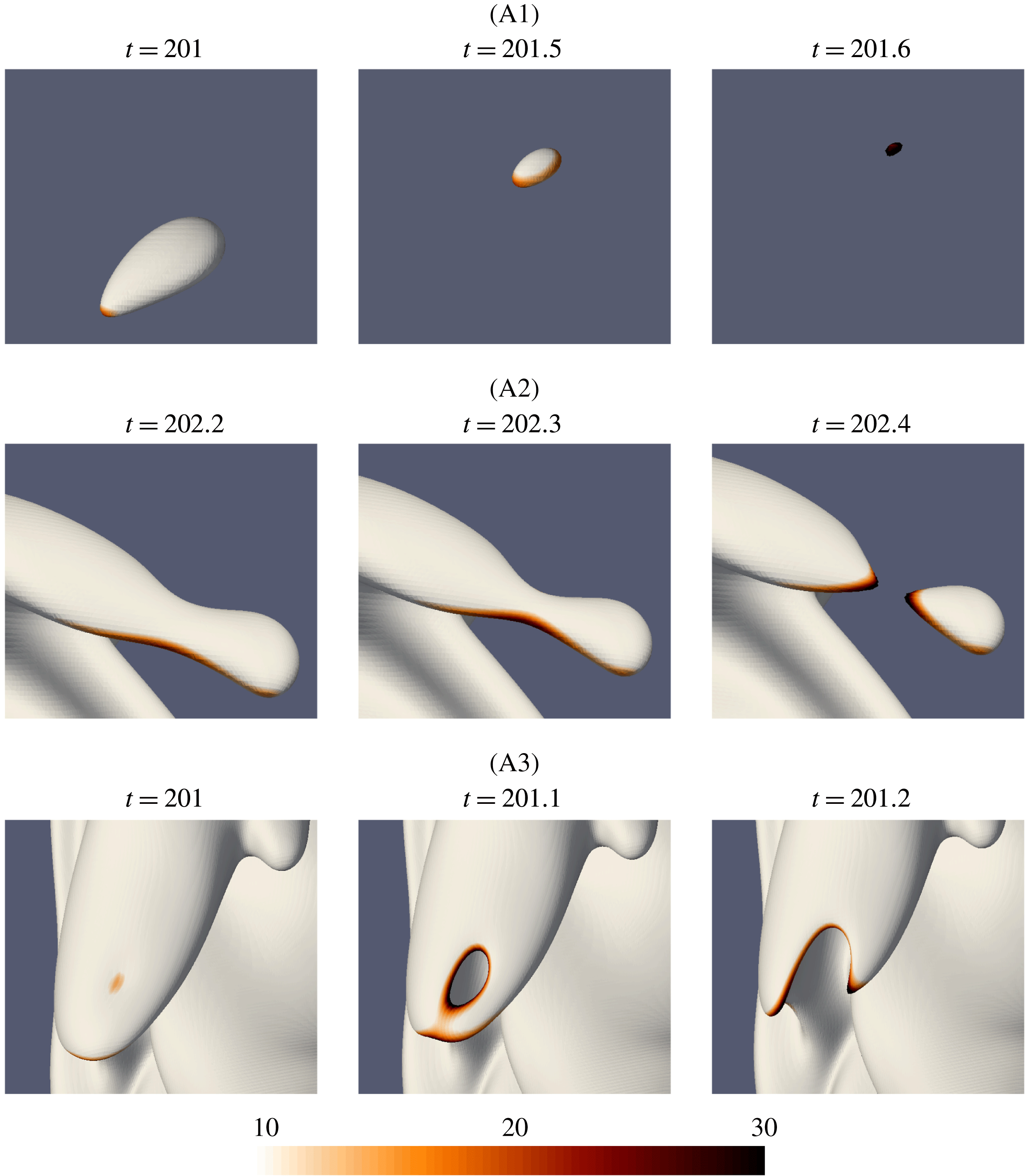
The time evolution of the three flame annihilation events labelled in figure 3 and their corresponding normalised density-weighted flame displacement speed (
 $S_{d}^{\ast }/S_{L}$
) fields mapped on the flame surface.

Figure 7 illustrates the iso-surface of the progress variable
 $Y_{R}=0.122$
corresponding to the three distinct flame annihilation events A1 to A3 in figure 3. These iso-surfaces are now coloured with the normalised density-weighted flame displacement speed (
 $S_{d}^{\ast }/S_{L}$
). There is a large increase in the magnitude of
 $S_{d}^{\ast }/S_{L}$
during the annihilation events. Thus,
 $S_{d}^{\ast }/S_{L}>10$
seems to be a reasonable condition for identifying annihilation events.
Figure 8 therefore shows scatter plots of grid nodes that satisfy this proposed identifier of flame annihilation, i.e. points with
 $Y_{R}=0.122$
for
 $\unicode[STIX]{x1D719}=1.0$
(
 $Y_{R}=0.156$
for
 $\unicode[STIX]{x1D719}=0.7$
) and
 $S_{d}^{\ast }/S_{L}>10$
. These scatter plots were generated using the same time period, which was the flow through time of the stoichiometric case detailed in table 1. Events throughout the stoichiometric and lean flames are evident and common. Perhaps surprisingly, the lean flame shows more of these events even though figures 3 and 6 showed that it was the quieter flame. However, this is not necessarily a contradiction, particularly since premixed flame noise is known to scale with the laminar flame speed (Smith & Kilham Reference Smith and Kilham1963; Strahle & Shivashankara Reference Strahle and Shivashankara1975; Talei et al.
Reference Talei, Brear and Hawkes2011). We therefore now consider how identification of these events can be used in a simple model of the radiated sound.
Time-averaged reaction rate and instantaneous scatter plot of nodes with
 $S_{d}^{\ast }/S_{L}>10$
on an iso-surface with (a)
 $Y_{R}=0.122$
for
 $\unicode[STIX]{x1D719}=1.0$
and (b)
 $Y_{R}=0.156$
for
 $\unicode[STIX]{x1D719}=0.7$
.

5 A simple model of sound generation by flame annihilation
We now consider a simple model of sound generation by these annihilation events. This model is consistent with the approach of Smith & Kilham (Reference Smith and Kilham1963), and considers the flame to be a distribution of annihilation events, each of which radiates monopolar sound to the far field. This simple model is therefore only a means of assessing the contribution of annihilation events to the overall sound produced by turbulent premixed flames, and is not intended to be a complete model of sound production since other sources are neglected.
5.1 Laminar flame annihilation
Spherically symmetric annihilation events are simulated first. The flame parameters are the same as those used in the turbulent flames for both stoichiometric and lean conditions. After initialising the flow field, the spherical flames start to propagate from their initial position at
 $r_{0}/\unicode[STIX]{x1D6FF}_{th}=7$
, where
 $r_{0}$
is the distance from the origin.
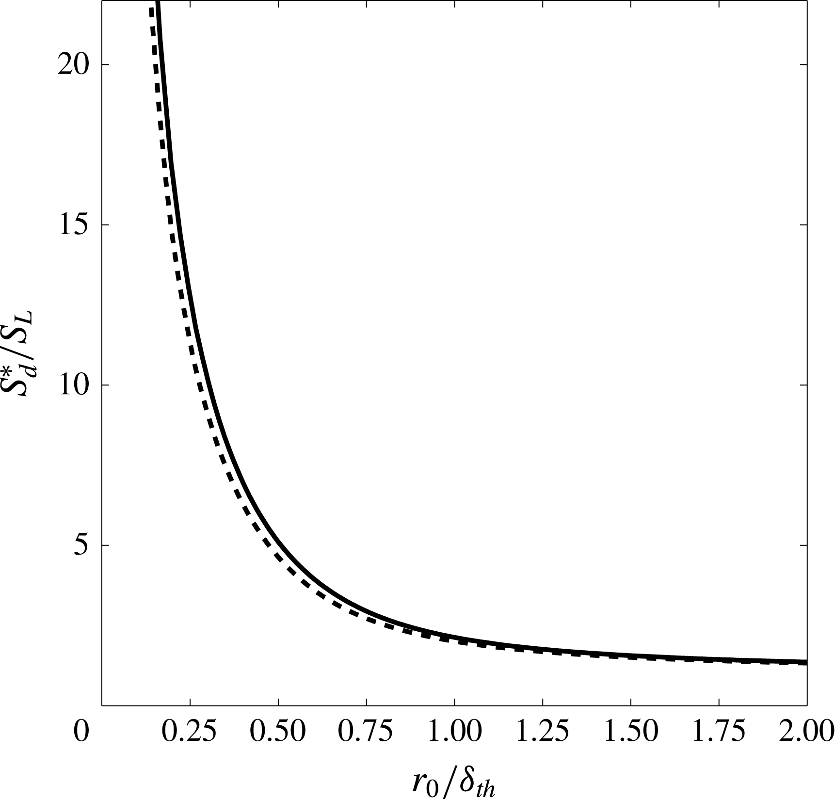
Figure 9 shows
 $S_{d}^{\ast }/S_{L}$
as a function of
 $r_{0}/\unicode[STIX]{x1D6FF}_{th}$
for both cases. It is observed that
 $S_{d}^{\ast }/S_{L}$
has a value of approximately unity when the flame is at
 $r_{0}/\unicode[STIX]{x1D6FF}_{th}\approx 2$
. After that,
 $S_{d}^{\ast }/S_{L}$
starts to increase, reaching very large values during annihilation, as several other studies have found (e.g. Echekki et al.
Reference Echekki, Chen and Gran1996; Sun & Law Reference Sun and Law1998).
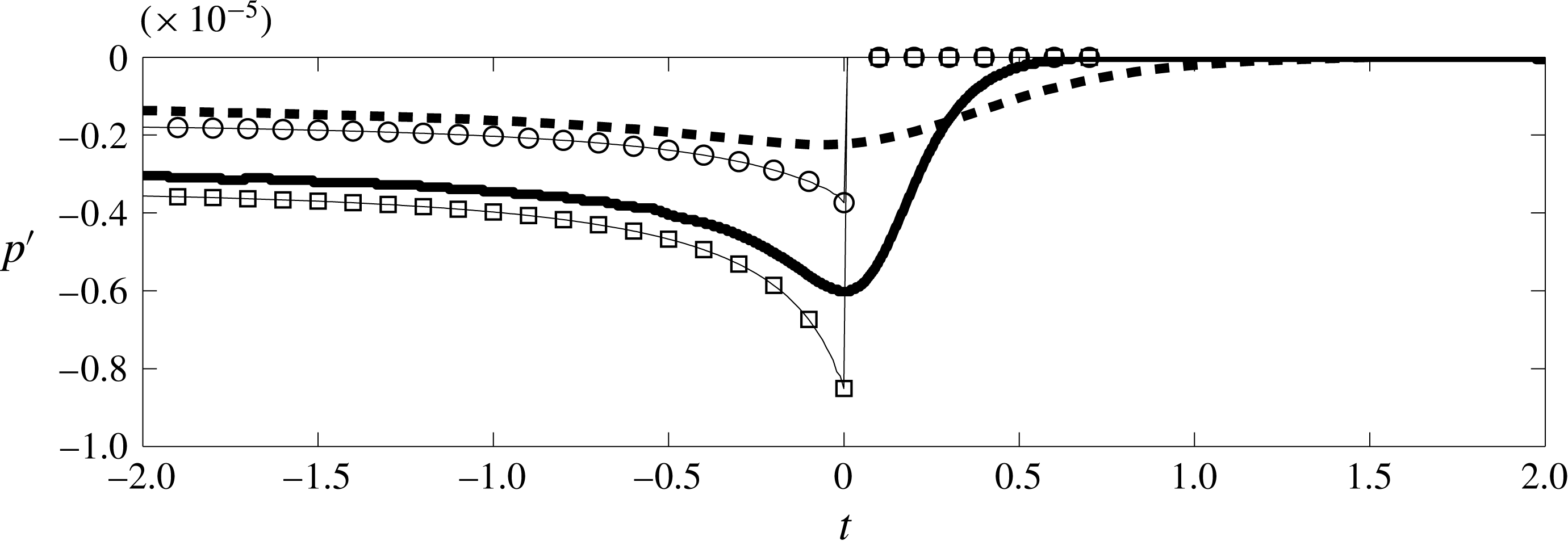
Figure 10 shows a comparison of the sound produced by both annihilation events at
 $r/\unicode[STIX]{x1D6FF}_{th}=28$
, where
 $r$
is the distance between the receiver and the centre of the flame sphere. The annihilation event corresponding to the lean flame is much quieter than that of the stoichiometric flame. This is consistent with Talei et al. (Reference Talei, Brear and Hawkes2011), who found that the sound produced for a spherically symmetric annihilation event is proportional to
 $S_{L}^{2}$
. This can also likely contribute to the lower level of noise produced by the turbulent lean flame.
Normalised density-weighted flame displacement speed (
 $S_{d}^{\ast }/S_{L}$
) as a function of normalised flame radius (
 $r_{0}/\unicode[STIX]{x1D6FF}_{th}$
) for a spherically symmetric annihilation event for
 $\unicode[STIX]{x1D719}=1.0$
(solid) and
 $\unicode[STIX]{x1D719}=0.7$
(dashed).

Time history of sound generated by a spherically symmetric annihilation event at
 $r/\unicode[STIX]{x1D6FF}_{th}=28$
from DNS for
 $\unicode[STIX]{x1D719}=1.0$
(solid) and
 $\unicode[STIX]{x1D719}=0.7$
(dashed) and by (5.1) for
 $\unicode[STIX]{x1D719}=1.0$
(square) and
 $\unicode[STIX]{x1D719}=0.7$
(circle).

5.2 Theory
Talei et al. (Reference Talei, Brear and Hawkes2012a ) used the theory of Dowling (Reference Dowling1992), which in turn extended Lighthill’s equation (Lighthill Reference Lighthill1952, Reference Lighthill1954), for the study of combusting flows. By considering the fluctuations in heat release as the only source term, modelling the reaction rate as a delta function and assuming a constant consumption speed, Talei et al. (Reference Talei, Brear and Hawkes2012a ) showed that the general solution of Lighthill’s equation for a spherically symmetric annihilation event is
 $$\begin{eqnarray}\displaystyle & \displaystyle p^{\prime }(r,t)=-2\unicode[STIX]{x1D70C}_{u}S_{L}\left(1-\frac{T_{u}}{T_{b}}\right)\frac{r_{0}(t-r/c_{b})}{r}V_{f}(t-r/c_{b})H(t-r/c_{b}), & \displaystyle\end{eqnarray}$$
where
 $p^{\prime }$
is the fluctuating part of the pressure,
 $c_{b}$
is the burned sonic speed,
 $H$
is the Heaviside function and
 $V_{f}$
is the magnitude of flame propagation velocity
 $\boldsymbol{V}_{f}$
projected onto the flame normal
 $\boldsymbol{n}$
,
 $$\begin{eqnarray}\displaystyle & \displaystyle V_{f}\equiv \boldsymbol{V}_{f}\boldsymbol{\cdot }\boldsymbol{n}=\boldsymbol{u}\boldsymbol{\cdot }\boldsymbol{n}+S_{d}. & \displaystyle\end{eqnarray}$$
Figure 10 compares
 $p^{\prime }$
from DNS and (5.1) for spherical annihilation events. The over-prediction of the peak pressure is due to the assumption of constant consumption speed, particularly at the later stages of the annihilation event (Talei et al.
Reference Talei, Brear and Hawkes2012a
). The step at the peak acoustic pressure in the theory is because the flame is represented as a delta function.
5.3 Model for turbulent premixed flames
5.3.1 Model description
Equation (5.1) provides a reasonable model of the noise generated by a single spherical annihilation event. However, this theory now needs to be extended to estimate sound generation by the various types of annihilation that occur throughout a turbulent flame. A precise extension of this equation to different types of annihilation events involves a substantial numerical and theoretical study to construct a model which incorporates the features of different types of annihilation events. This is beyond the scope of this work. Thus, as a first step, all annihilation events are assumed to be spherically symmetric, and the simplification in making this assumption must always be kept in mind.
The iso-surface of the progress variable corresponding to the maximum reaction rate (
 $Y_{R}=0.122$
and
 $0.156$
for
 $\unicode[STIX]{x1D719}=1.0$
and
 $\unicode[STIX]{x1D719}=0.7$
respectively) are then conditioned using
 $S_{d}^{\ast }/S_{L}\geqslant n$
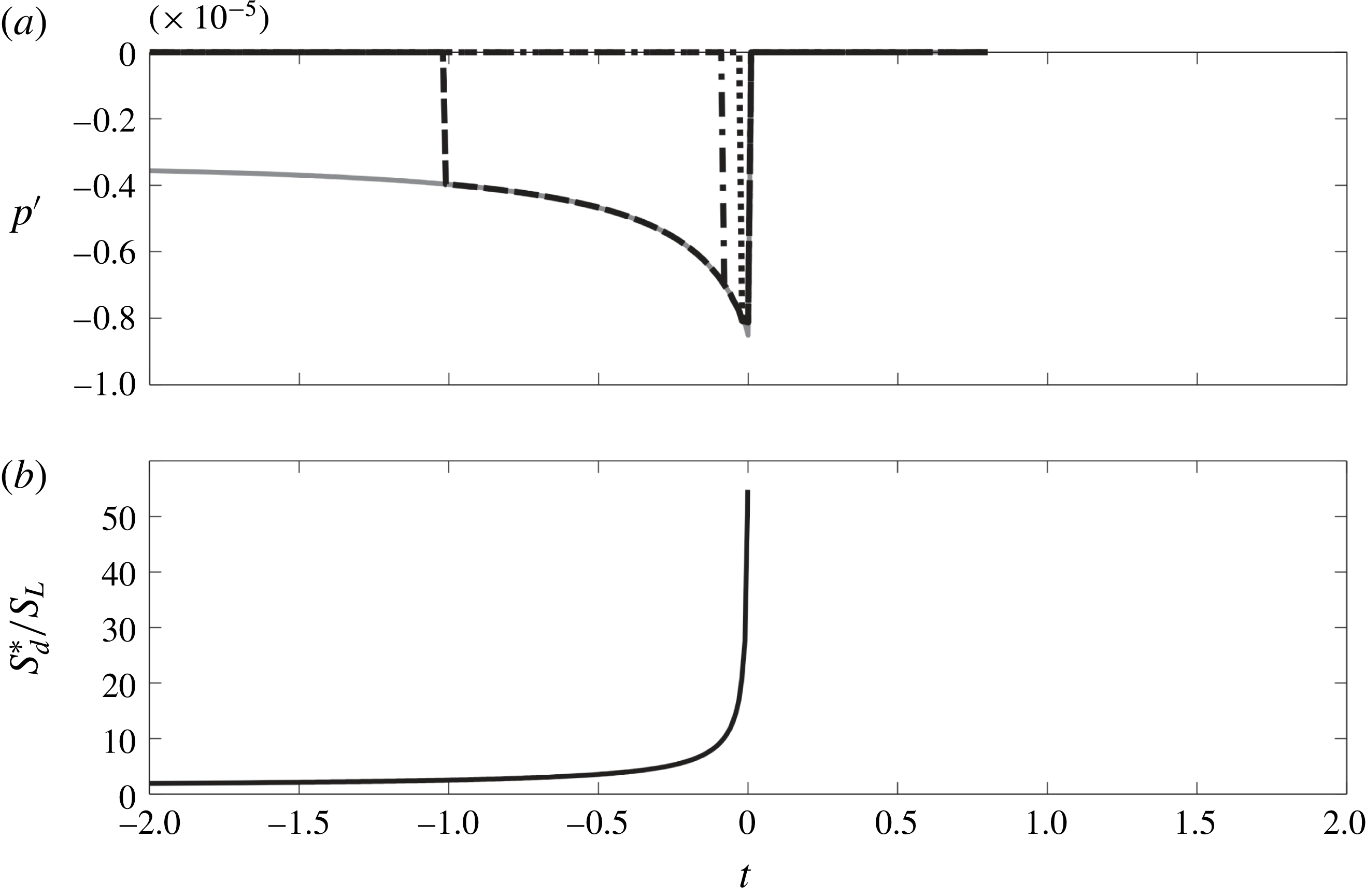
as a marker. Figure 11 shows the effect of different values of
 $n$
on the noise generated by a spherically symmetric annihilation event using a modified form of (5.1),
 $$\begin{eqnarray}\displaystyle \displaystyle p^{\prime }(r,t) & = & \displaystyle -2\unicode[STIX]{x1D70C}_{u}S_{L}\left(1-\frac{T_{u}}{T_{b}}\right)\frac{r_{0}(t-r/c_{b})}{r}V_{f}(t-r/c_{b})\nonumber\\ \displaystyle & & \displaystyle \times \,H(t-r/c_{b})H\left({\displaystyle \frac{S_{d}^{\ast }(t-r/c_{b})}{S_{L}}}-n\right).\end{eqnarray}$$
The rightmost Heaviside function in (5.3) is added to capture annihilation events. As mentioned earlier, flame acceleration is a defining feature of these events. We therefore use this function to identify annihilation by setting a threshold on
 $S_{d}^{\ast }/S_{L}=n$
. It can be seen that when
 $n=2.5$
is chosen, the whole annihilation is captured whereas for
 $n=20$
, only the final stage of annihilation is recovered. Equation (5.3) requires the information at
 $t-r/c_{b}$
for each annihilation event. This instant might not coincide with the instants at which the DNS data are collected. We therefore used a time shift
 $r/c_{b}$
to obtain the pressure fluctuations at a later time as follows:
 $$\begin{eqnarray}\displaystyle & \displaystyle p^{\prime }(r,\unicode[STIX]{x1D70F}+r/c_{b})=-2\unicode[STIX]{x1D70C}_{u}S_{L}\left(1-\frac{T_{u}}{T_{b}}\right)\frac{r_{0}(\unicode[STIX]{x1D70F})}{r}V_{f}(\unicode[STIX]{x1D70F})H\left({\displaystyle \frac{S_{d}^{\ast }(\unicode[STIX]{x1D70F})}{S_{L}}}-n\right), & \displaystyle\end{eqnarray}$$
where
 $\unicode[STIX]{x1D70F}=t-r/c_{b}$
and
 $r_{0}$
is determined from figure 9 at a given
 $S_{d}^{\ast }/S_{L}$
.
(a) Comparison of the sound generated by a spherically symmetric annihilation event at
 $r/\unicode[STIX]{x1D6FF}_{th}=28$
using (5.1) (solid) and the modified theory (equation (5.3)) with
 $n=2.5$
(dashed), 10 (dash-dot) and 20 (dotted). (b) The corresponding time history of
 $S_{d}^{\ast }/S_{L}$
for this event.

(a) One snapshot of the flame iso-surface for
 $\unicode[STIX]{x1D719}=1.0$
on a uniform mesh with a cube of edge length
 $\unicode[STIX]{x1D6E5}=2\unicode[STIX]{x1D6FF}_{th}$
. (b) The regions B1, B2 and B3 in (a) are zoomed in and coloured with the
 $S_{d}^{\ast }/S_{L}$
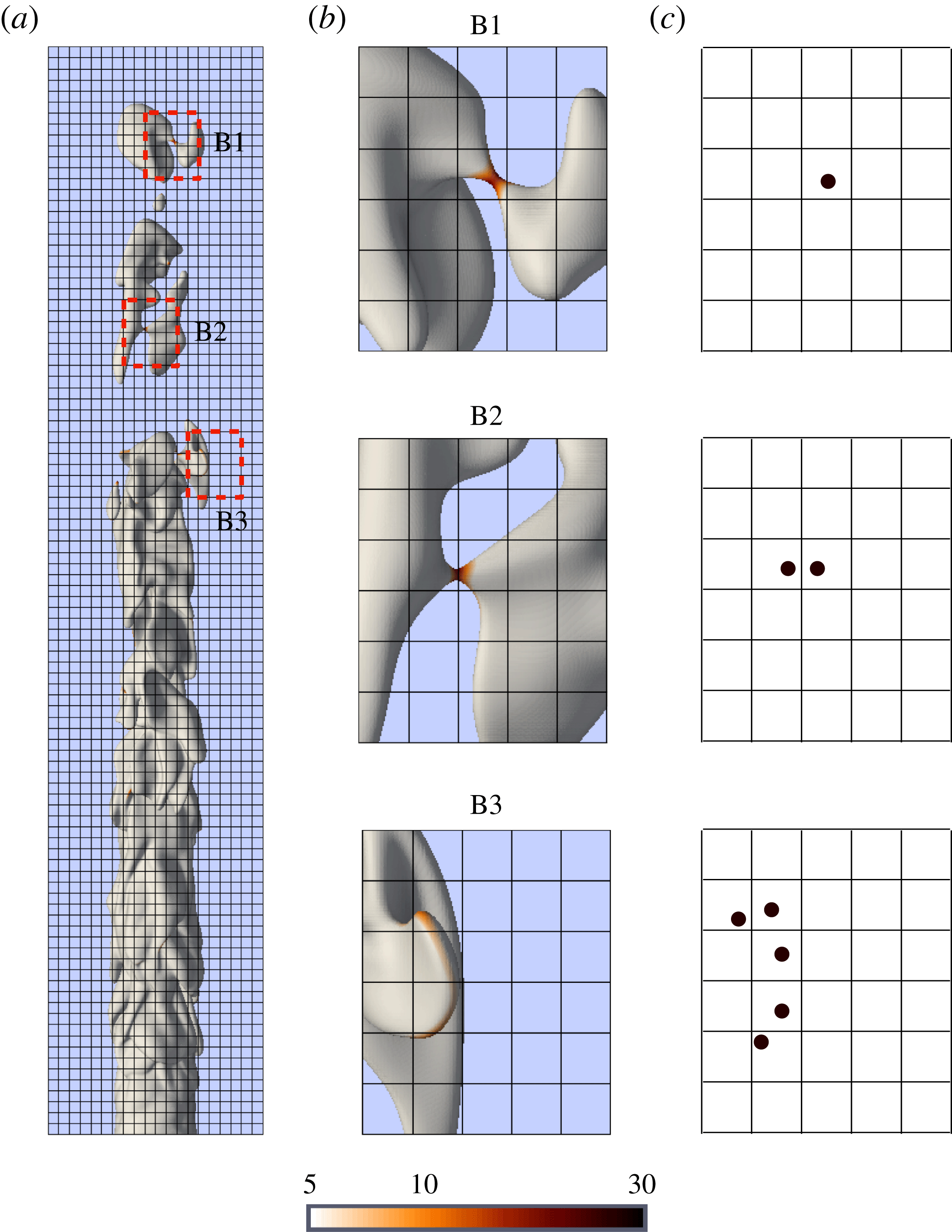
field. (c) Centroid of the cluster of the conditioned data as per § 5.3.2.

5.3.2 Algorithm
There are four steps in our modelling algorithm.
(i) Divide the domain into cubes.
(ii) Identify flame annihilation events.
(iii) Represent the flame with a number of spherically symmetric annihilation events.
(iv) Calculate the total sound produced.
Figure 9 shows that having information from the instant at which
 $r_{0}=\unicode[STIX]{x1D6FF}_{th}$
is sufficient to represent the annihilation event. Note that
 $r_{0}=\unicode[STIX]{x1D6FF}_{th}$
corresponds to
 $S_{d}^{\ast }/S_{L}\approx 2.5$
which is the lowest threshold for
 $S_{d}^{\ast }/S_{L}$
considered in this study. We therefore assume that each cube in the domain has a size of
 $2\unicode[STIX]{x1D6FF}_{th}$
in which only one spherically symmetric annihilation event can occur at any time. The entire domain that features the flame is therefore divided into these uniformly distributed cubes (figure 12
a).
For step 2, the points on the iso-surfaces of
 $Y_{R}$
(0.122 and 0.156 for the stoichiometric and the lean cases, respectively) in each cube with
 $S_{d}^{\ast }/S_{L}\geqslant n$
and
 $V_{f}>0$
are identified at each instant. Figure 12(b) shows examples of the identified points for different types of annihilation events.
For step 3, the cluster of points in each cube is now replaced with one point at the centroid of the cluster with an averaged propagation velocity obtained from the velocity of each point. This point is considered as one spherically symmetric annihilation event. Figure 12(c) shows how the flame pinch-off event labelled as B1 is represented by one spherically symmetric annihilation. Another flame pinch-off event labelled as B2 is considered as two events since it is split into two cubes. Although this event is very similar to that labelled as B1, it will be modelled as a sound source of twice the strength. This is an unavoidable and undesirable feature of this algorithm, with some over-prediction of the sound expected to result. Finally, the event labelled as B3 shows a long, curved flame edge distributed over several cubes. Once again, this will potentially contribute to over-prediction of the sound.
Step 4 then calculates the overall sound produced by calculating the noise generated by each annihilation event. First, a number of time bins (with the bin size equal to the sampling size of the DNS data) are considered and the result of (5.4) for each representative point source is stored in its associated time bin. Then,
 $p^{\prime }$
in the far field resulting from the sound produced by all points is calculated by summing the stored values in each time bin.
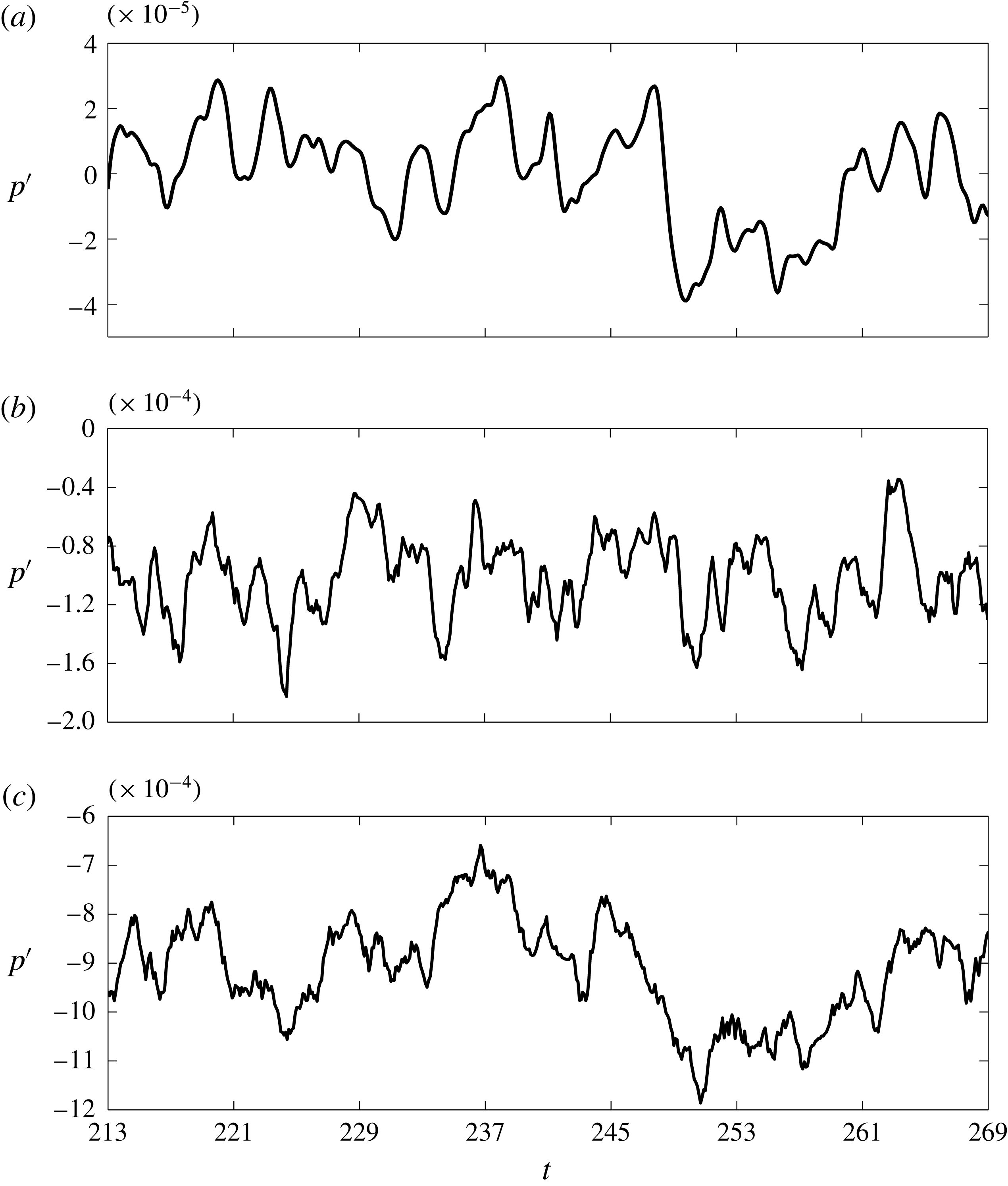
Time history of the far-field noise at
 $r=6D$
and
 $x=10D$
for
 $\unicode[STIX]{x1D719}=1.0$
, obtained from (a) DNS, (b) model with
 $n=10$
and (c) model with
 $n=5$
.

5.4 Comparison of the simple model with DNS
Figure 13(a) depicts the time history of the acoustic pressure
 $p^{\prime }$
at
 $x=10D$
and
 $r=6D$
(One should note that since the relevant length scale for annihilation events is the flame thickness, the receiver
 $r=85\unicode[STIX]{x1D6FF}_{th}$
is sufficiently far from the jet to be considered in the far field, as our previous studies of laminar flames have shown (Talei et al.
Reference Talei, Brear and Hawkes2011, Reference Talei, Brear and Hawkes2012a
).) obtained from the DNS for the case with
 $\unicode[STIX]{x1D719}=1.0$
. Figure 13(b,c) shows the corresponding model results for
 $n=10$
and
 $5$
, respectively. The modelled signals contain some high frequency noise which is due to the model representing the flame as discrete point sources that appear and disappear rapidly due to the conditioning on
 $S_{d}^{\ast }/S_{L}$
. The correlation coefficient,
 $\unicode[STIX]{x1D70C}=\text{cov}(X,Y)/(\unicode[STIX]{x1D70E}(X)\unicode[STIX]{x1D70E}(Y))$
, between the modelled signal and the DNS data is 36 % for
 $n=10$
and 66 % when
 $n=5$
is used. A comparison of figures 13(b,c) and 13(a) also shows that the magnitude of the pressure fluctuations is over-predicted by the model, as discussed in § 5.3.2. Clearly, the choice of threshold
 $n$
is important.
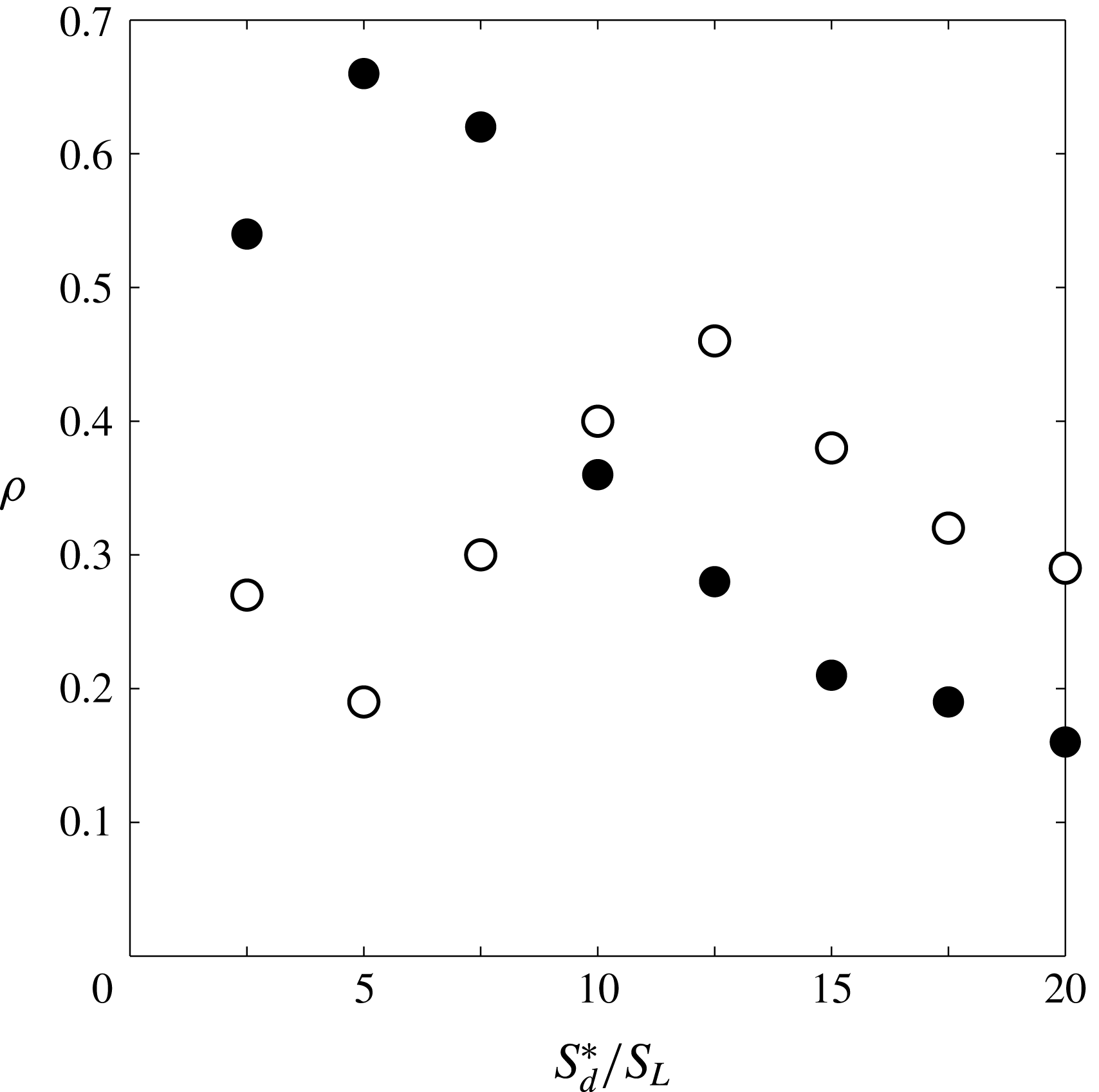
Correlation coefficient
 $\unicode[STIX]{x1D70C}$
between the DNS far-field noise and that of the model at
 $r=6D$
and
 $x=10D$
as a function of
 $S_{d}^{\ast }/S_{L}$
for
 $\unicode[STIX]{x1D719}=1$
(solid circles) and
 $\unicode[STIX]{x1D719}=0.7$
(hollow circles).

A range of
 $n$
from 2.5 to 20 is therefore considered. For high values of
 $n$
, some of the annihilation events are not captured because of the finite time resolution of the recorded DNS data. On the other hand, choosing a low value of
 $n$
will include parts of the flame surface which are not annihilation events. This suggests that there will be an optimum value of
 $n$
in terms of correlation coefficient. Figure 14 supports this hypothesis by showing that
 $n=5$
and
 $n=12.5$
are optimal for the stoichiometric and lean cases, respectively. The optimal correlation is particularly strong for the stoichiometric flame, demonstrating the significant contribution of annihilation events to sound production.
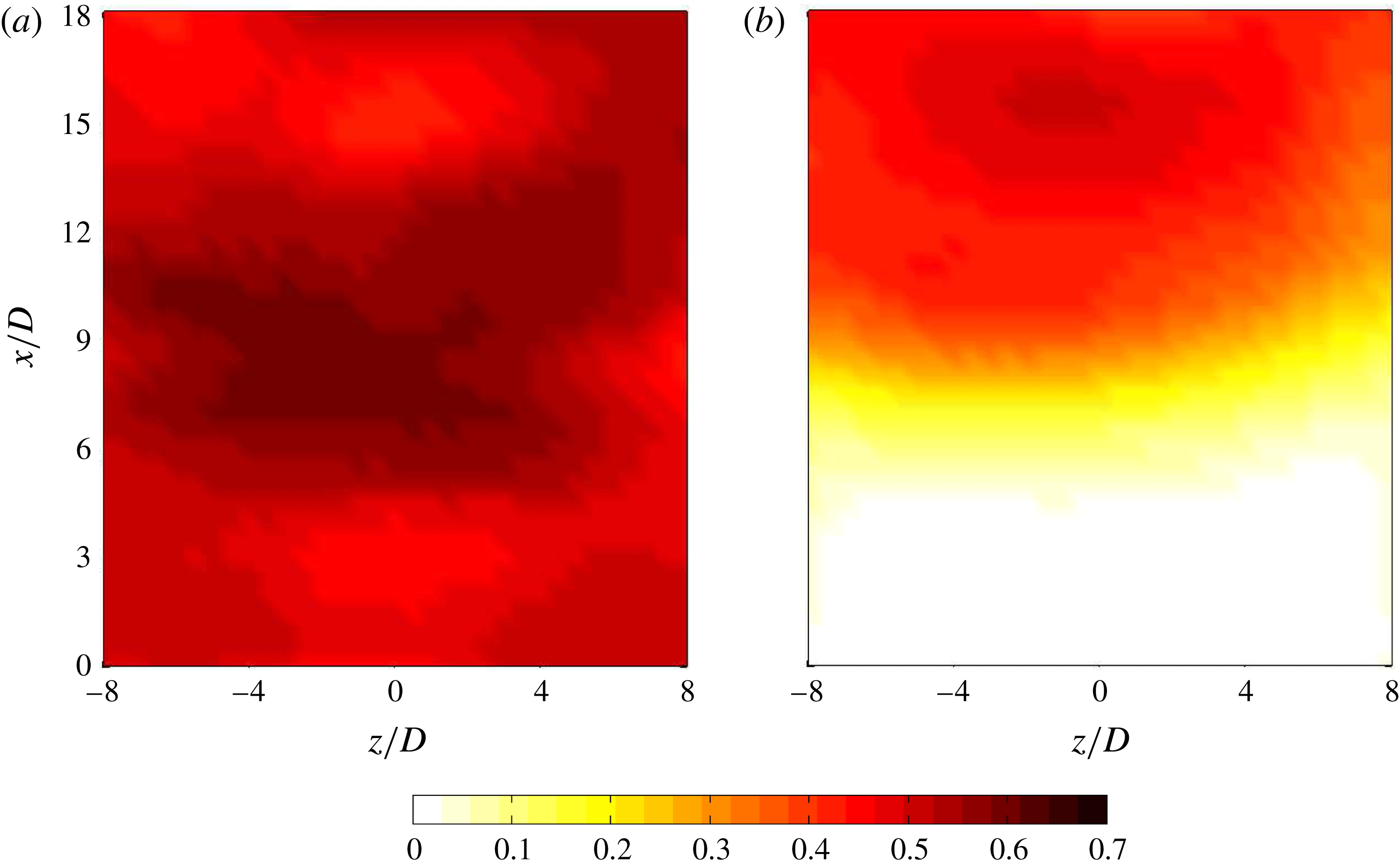
Figure 15 shows this correlation coefficient over an
 $x{-}z$
plane located at
 $y/D=-6$
. The optimum values of
 $n$
for both flames in figure 14 are used to calculate the correlation coefficient. While an almost uniform distribution is observed for the stoichiometric flame (figure 15
a), two distinct zones are found for the lean flame (figure 15
b). This shows that annihilation events are a strong source of noise for the stoichiometric flame. There is, however, a competition between the sound produced by the annihilation events and other sources such as the inflow noise for the quieter, lean flame.
Distribution of the correlation coefficient
 $\unicode[STIX]{x1D70C}$
between the DNS and the model calculated over an
 $x{-}z$
plane located at
 $y/D=-6$
for (a)
 $\unicode[STIX]{x1D719}=1.0$
with
 $n=5$
and (b)
 $\unicode[STIX]{x1D719}=0.7$
with
 $n=12.5$
.

The degree of correlation between the DNS and the model in figure 15 is surprising given the model’s simplicity. The model considers all sound sources to be spherically symmetric annihilations, even though other forms of annihilation were shown to exist and other sound sources are expected in combusting flows (Dowling Reference Dowling1992; Talei et al. Reference Talei, Brear and Hawkes2014). Further, all sound is modelled as travelling radially from these sources at the burnt gas velocity, ignoring refraction and sound propagation at lower velocity, as should occur for a source on one side of the flame with the receiver on the other side.
Smith & Kilham’s (Reference Smith and Kilham1963) model of a flame as a distribution of monopolar sound sources therefore appears to be insightful. The simple model in the present work identifies flame annihilation events as these sources and, in so doing, provides a physical explanation for the well-known monopolar content of the sound radiated by premixed turbulent flames.
6 Conclusions
This paper presented a numerical study of the sound generated by turbulent, premixed flames. Direct numerical simulations (DNS) of two round jet flames with equivalence ratios of 0.7 and 1.0 were first carried out. Single-step chemistry was employed to reduce the computational cost, and care was taken to resolve both the near and far fields and to avoid noise reflections at the outflow boundaries.
Several significant features of these two simulated flames were noted. First, the acoustic fields of both the stoichiometric and lean flames exhibited monopolar features that originated within the flame, with the stoichiometric flame being significantly louder than the lean flame. These observations are consistent with several experimental studies of turbulent jet flames in the literature. Further, so-called ‘flame annihilation’ events were observed to be a source of these monopolar, acoustic features, which was consistent with prior works on laminar premixed flames. The acoustic spectra of both flames were also studied. These were found to be broadband in nature, with a frequency at the peak spectral amplitude agreeing with those observed experimentally by Rajaram & Lieuwen (Reference Rajaram and Lieuwen2009).
A simple model that related the observed annihilation events to the far-field sound was then proposed. This model considered the far-field sound as the superposition of the sound radiated by individual, spherically symmetric annihilation events that occurred throughout the flame. These events were identified by conditioning the flame displacement speed at some threshold since flame annihilation is well known to feature flame acceleration. The choice of threshold was shown to strongly affect the correlation between the modelled and measured, far-field sound, with the correlation coefficient exceeding 0.5 in some cases. Such levels of correlation were surprising given the model’s simplicity, and demonstrated the importance of flame annihilation as acoustic sources in turbulent premixed flames. This model is also consistent with Smith & Kilham’s (Reference Smith and Kilham1963) model of a flame as a distribution of monopolar sound sources, with the present work identifying flame annihilation events as these sources and, in so doing, providing a physical explanation for the well-known monopolar content of the sound radiated by premixed turbulent flames.
Acknowledgements
This study was supported by the Advanced Centre for Automotive Research and Testing (ACART, www.acart.com.au), the Australian Research Council (ARC) and the Australian Government’s National Computational Merit Allocation Scheme. The computational facilities supporting this project included the Australian National Facility (NCI), the partner share of the NCI facility provided by Intersect Australia Pty Ltd. and the Pawsey Supercomputing Centre.
Supplementary material
Supplementary material is available at https://doi.org/10.1017/jfm.2018.115.