1 Introduction
Liquid impact phenomena are ubiquitous in science, nature and technology. They are critically important in fields ranging from biotechnology and agriculture to marine engineering. One particular phenomenon observed in liquid impacts on solid surfaces is that of splashing, where the wetting front propagating along the surface becomes unstable, detaches from the surface, and can subsequently disperse into multiple smaller droplets. Several causes of splashing initiation have been identified: for example, surface roughness and interaction of the fast-moving wetting jet with the surrounding air. Controlling splashing is of practical interest. When designing a car windscreen, splashing is encouraged to disperse rain (Blocken & Carmeliet Reference Blocken and Carmeliet2004), whilst splashing should be avoided in ink-jet printing (Martin, Hoath & Hutchings Reference Martin, Hoath and Hutchings2008). Increasingly surfaces are being designed using smart materials or with microstructured roughness to control droplet dynamics (Maitra et al. Reference Maitra, Antonini, Tiwari, Mularczyk, Imeri, Schoch and Poulikakos2014a ,Reference Maitra, Tiwari, Antonini, Schoch, Jung, Eberle and Poulikakos b ). Splashing is a complicated process governed by several physical effects. It is determined by properties of the liquid, substrate and surrounding atmosphere. Flexibility of the substrate is another physical effect which may cause splashing. This effect has can be observed for substrates with relatively high rigidity.
Despite the importance of splashing, the mechanisms that trigger splashing are still not fully understood. It was discovered in experiments carried out by Xu, Zhang & Nagel (Reference Xu, Zhang and Nagel2005) that the pressure of the surrounding gas was critically important for the splashing of a drop impacting a smooth surface. Xu (Reference Xu2007) later experimentally studied the impact of liquid drops with a variety of surfaces, and found that the surrounding gas is responsible for ‘corona’ splash where the rapidly spreading liquid can detach from the wall and substrate roughness causes ‘prompt’ splash characterised by the creation of smaller droplets at the contact line. Riboux & Gordillo (Reference Riboux and Gordillo2014) studied the effects of the presence of surrounding gas in droplet impacts onto smooth surfaces, deriving a relationship between splashing and a critical impact velocity. Ellis, Smith & White (Reference Ellis, Smith and White2011) analytically investigated the impact of a liquid droplet with a rough surface using the Wagner model for a surface of small roughness, and an alternative model for rougher surfaces. Their study did not incorporate splashing, but the analysis showed that the effect of surface roughness can be modelled in an appropriate small-roughness limit.
Whilst previous theoretical works have focused on the air and surface roughness as the causes of splashing, here we will show that elasticity of the impacted substrate is an additional mechanism for splashing. It has been shown experimentally that elasticity can play a key role in splashing. Pepper, Courbin & Stone (Reference Pepper, Courbin and Stone2008) presented an experimental study of droplets impacting an elastic membrane held under different tensions. They found indications that it is the very early times after impact that are critical for determining whether splashing will occur. They showed that a soft substrate can suppress splashing entirely. Experimental studies (see, for example, Mangili et al. Reference Mangili, Antonini, Marengo and Amirfazli2012 and Alizadeh et al. Reference Alizadeh, Bahadur, Shang, Zhu, Buckley, Dhinojwala and Sohal2013) of droplets impacting deformable surfaces have focused on soft surfaces. Experiments of droplet impacts onto soft silicone and acrylic substrates were performed by Howland et al. (Reference Howland, Antkowiak, Castrejón-Pita, Howison, Oliver, Style and Castrejón-Pita2016). Like Pepper et al. (Reference Pepper, Courbin and Stone2008), they found softer substrates caused a reduction in the splashing threshold.
Our current analytical and numerical study is based on the Wagner model of liquid impact. It was first developed by Wagner (Reference Wagner1932) for evaluating the hydrodynamic loads on the floaters of seaplanes during landing. The Wagner model assumes that the solid surface and the free surface of the liquid at impact are nearly parallel to each other, with the normal displacements of these surfaces being much smaller than the size of their contact region. The Wagner model is used during the early stages of impact, when the geometry of the impacting surfaces, equations of the liquid flow, and the corresponding boundary conditions can be simplified. However, the problem remains nonlinear because the size of the wetted area is unknown in advance and should be determined as part of the solution. The size of the wetted part of the substrate is determined by using the so-called Wagner condition. This condition requires that the liquid boundary, which includes the liquid free surface and the wetted area of the substrate, is continuous. This condition was formally justified by Howison, Ockendon & Wilson (Reference Howison, Ockendon and Wilson1991) through an asymptotic analysis of liquid impact problems.
Many of the studies adopting the Wagner model have focused on two-dimensional problems. A droplet–liquid impact problem was investigated by Howison et al. (Reference Howison, Ockendon, Oliver, Purvis and Smith2005). Water entry problems (mathematically equivalent to droplet impact) have received much more attention, stretching as far back as the studies by von Karman (Reference von Karman1929), who investigated the impact of a solid wedge onto a water free surface. Other examples include Wu (Reference Wu2007), who investigated the impact of liquid columns and droplets on solid wedges, and Philippi, Lagree & Antkowiak (Reference Philippi, Lagree and Antkowiak2016), who investigated the early stages of a liquid drop impacting with a solid plate. Liquid–liquid impacts were investigated by Semenov, Wu & Korobkin (Reference Semenov, Wu and Korobkin2015). There have been a considerable range of other important effects considered, including three-dimensional oblique impact (Moore et al. Reference Moore, Howison, Ockendon and Oliver2012), water entry of a skimming elastic plate (Reinhard, Korobkin & Cooker Reference Reinhard, Korobkin and Cooker2013), as well as including air cushioning effects (Moore, Ockendon & Oliver Reference Moore, Ockendon and Oliver2013; Moore & Oliver Reference Moore and Oliver2014). Liquid-elastic impacts have begun to receive an increasingly large amount of attention. Khabakhpasheva & Korobkin (Reference Khabakhpasheva and Korobkin2013) investigated the two-dimensional liquid-elastic wedge impact problem and Tkacheva (Reference Tkacheva2008) studied the impact of a box with an elastic base onto a thin layer of liquid. Many of the papers studying the three-dimensional impact problem derive from the work presented by Scolan & Korobkin (Reference Scolan and Korobkin2001) and Korobkin & Scolan (Reference Korobkin and Scolan2006). Xu, Wu & Duan (Reference Xu, Wu and Duan2011) investigated the axisymmetric impact of a liquid block onto a solid surface and Scolan (Reference Scolan2004) has produced one of the few works on an axisymmetric liquid-elastic impact.
The present study addresses the normal impact between an axisymmetric liquid droplet and a circular elastic plate which sits, simply supported, within an otherwise rigid flat surface. The radius of the elastic plate is taken to be much smaller than the radius of the liquid droplet. Aside from splashing mechanisms being of fundamental theoretical interest, increasingly designs of microfluidic devices are investigating and making use of such small flexible elements. For example, Nguyen, Takahashi & Shimoyama (Reference Nguyen, Takahashi and Shimoyama2017) report on the design of a pressure sensor using a small (centimetre scale) flexible polydimethylsiloxane (PDMS) membrane for measuring droplet vibrations. Vasileiou, Schutzius & Poulikakos (Reference Vasileiou, Schutzius and Poulikakos2017) performed experiments on supercooled droplets impacting upon a superhydrophobic flexible substrate. They found that a flexible patterned substrate (of approximate dimensions 30 mm) could repel supercooled droplets which would freeze on an equivalent rigid substrate. Weisensee et al. (Reference Weisensee, Tian, Miljkovik and King2016) investigated droplets impacting and bouncing off elastic superhydrophobic surfaces. They found that the contact time of a bouncing droplet is dramatically reduced with the introduction of an elastic substrate of size approximately 10 mm. Although these experiments considered droplets of comparable size to the flexible substrates, they demonstrate a trend towards the attempted understanding and development of small-scale surface structures and nanoengineered surfaces (see also Maitra et al. Reference Maitra, Antonini, Tiwari, Mularczyk, Imeri, Schoch and Poulikakos2014a ,Reference Maitra, Tiwari, Antonini, Schoch, Jung, Eberle and Poulikakos b ). The use of such elastic substrates allows for the creation of unique devices and opens up an additional way to control droplet wetting, impact, bouncing and, as we show in this work, potentially splashing.
Many of the recent studies showing that flexible or deformable substrates suppress splashing, such as those by Pepper et al. (Reference Pepper, Courbin and Stone2008) and Howland et al. (Reference Howland, Antkowiak, Castrejón-Pita, Howison, Oliver, Style and Castrejón-Pita2016), consider regimes where the time scales of any response from the substrate are much longer than those associated with the initial stages of the droplet splash. The configuration we present here is chosen such that, rather than just absorbing energy during the initial, most violent, part of the impact, the substrate is genuinely interacting over the same initial time scale. We concentrate on a parameter regime where the plate has a relatively high rigidity so that, rather than simply being deformed by the impact, it can vibrate. The period of the substrate vibration is of the order of the duration of the impact stage, and deflections of the elastic plate remain small. Vibration of the substrate and the liquid flow in the impacting droplet are coupled through the hydrodynamic pressure and the kinematic boundary condition on the wetted part of the substrate. The effects of viscosity, surface tension and gravity are shown to play a negligible role during the early stages of impact. We assume the conditions are such that the flow caused by the impact is driven by inertia, and described by the theory of potential flow. The gas surrounding the droplet is also not taken into account.
The flow in the main part of the droplet, deflection of the elastic plate, and the size of the wetted area are described by the model of Wagner (Reference Wagner1932). The plate vibrations are described by the method of normal modes. The two-dimensional study by Korobkin & Khabakhpasheva (Reference Korobkin and Khabakhpasheva2006) used this method to investigate the impact of a water wave onto an elastic plate. In contrast to the current paper, the entire focus of Korobkin & Khabakhpasheva (Reference Korobkin and Khabakhpasheva2006) was to predict the loads experienced by the plate due to impact; other than noting that the splash jets exist, the characteristics of the splash, and in particular how the elasticity of the plate drives the splash, were not considered. Scolan (Reference Scolan2004) used the method of normal modes to investigate an elastic cone impacting a liquid. The present analysis, unlike those works, focuses on the jetting and initiation of splashing. The Wagner model provides the speed of the jet formed at the periphery of the wetted surface, and the thickness of the jet through the self-similar and nonlinear solution of the impact problem in the jet-root region (Howison et al. Reference Howison, Ockendon and Wilson1991). The speed of the jet is a monotonically decreasing function of time for a rigid substrate, but can be non-monotonic for an elastic substrate. The dynamics of the jet is described by a system of nonlinear hyperbolic shallow-water equations. These equations predict a gradient catastrophe if the flow speed at the entrance to the jet is a non-monotonic function of time. This blow-up of the jet solution strongly indicates the onset of splashing with formation of a corona at some distance from the jet-root region. In this paper the role of elasticity on splashing is highlighted and quantified. We note here that we adopt an axisymmetric model to allow better comparison with experimental results in the future. The new splashing mechanism identified here would also be present in two-dimensional configurations.
In § 2 below, we introduce the problem of a droplet impacting upon a substrate which includes a small elastic part. We introduce the relevant scales and non-dimensional variables for the early stage of droplet impact within a potential flow model. Both the coupled elastic and hydrodynamic problems are described at the leading order. These problems are coupled, in particular, via the equation for the unknown radius of the contact region between the droplet and substrate. The resulting model is based on the Wagner theory of liquid impact. In § 3, the plate deflection is obtained by the normal mode method and the hydrodynamic pressure in the contact region is determined as a solution of an axisymmetric mixed boundary value problem for the velocity potential of the flow in the droplet. The obtained solution predicts singular flow velocities close to the advancing contact line. The Wagner solution is corrected near the contact region in § 4, where the jet-root region is introduced. The solution of the problem in the jet-root region provides the speed of the flow at the entrance to the jet and the thickness of this sheet. The jet flow is described by a one-dimensional nonlinear model. It is shown that the nonlinear jet solution breaks down if the acceleration of the contact line is positive, predicting unbounded jet thickness. This is interpreted as splashing. In § 5, the coupled problem of hydroelasticity is solved numerically. Convergence and stability of the numerical algorithm are discussed. The results of the analysis are presented in § 6. It is shown that the Wagner model of liquid impact is no longer appropriate for very thin plates, or for very flexible plates. Conditions of splashing are obtained and explained. The conclusions are drawn in § 7 together with ideas for future work. For clarity, some details of the analysis are collected in the appendices at the end of the paper.
2 Formulation of the problem
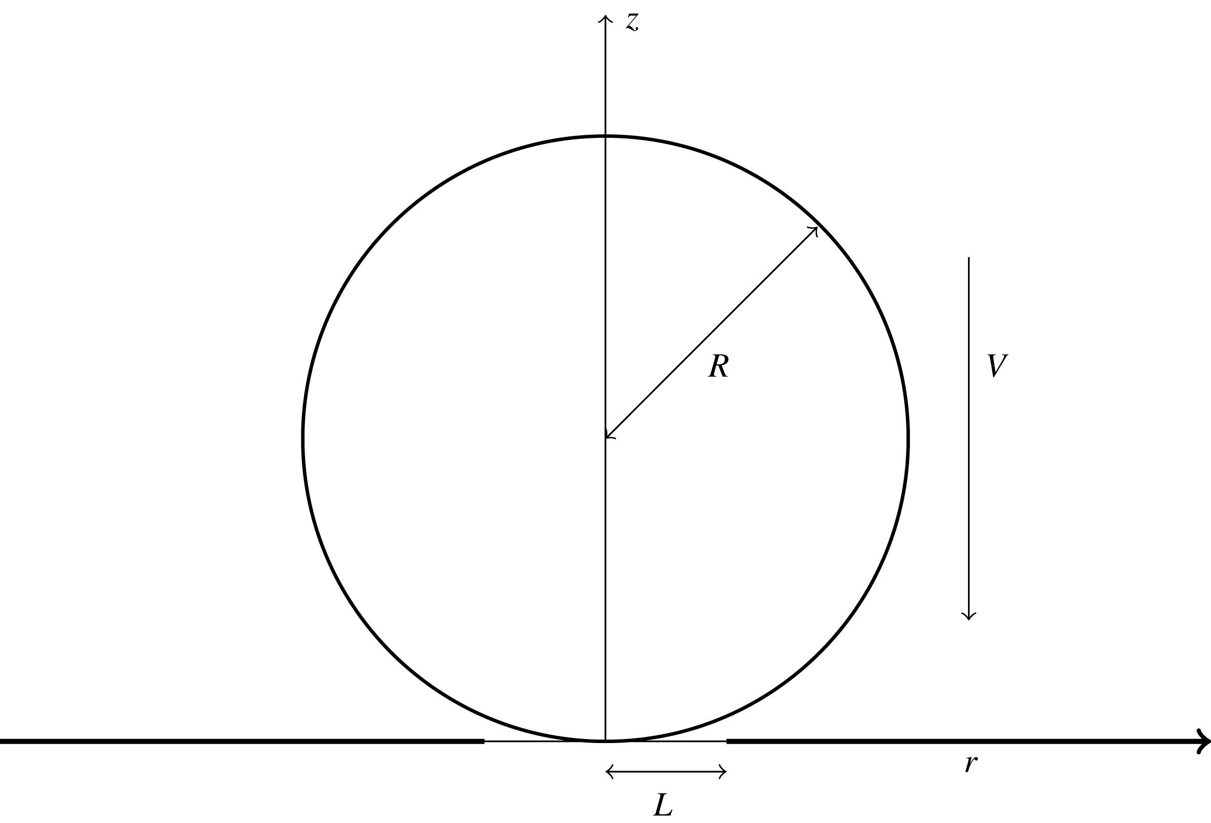
A side-on view of the problem. A spherical droplet of radius
 $R$
, travelling with constant speed
 $V$
, impacts onto a circular elastic plate of radius
 $L$
(thin horizontal line) housed in a solid housing of otherwise infinite extent (thick horizontal line).

The axisymmetric problem of a liquid droplet impacting onto a partly elastic substrate is formulated in non-dimensional variables. The liquid drop is taken to be spherical before impact, with radius
 $R$
. The impact speed
 $V$
is constant. At the instant of impact
 $(t=0)$
, the drop touches the elastic circular plate at its central point. The circular elastic plate of radius
 $L$
sits in an otherwise rigid substrate, and is simply supported at its edge (see figure 1). The liquid in the drop is assumed inviscid and incompressible, and the subsequent flow is irrotational and axisymmetric. The effects of the surrounding gas, gravity and surface tension are neglected; these assumptions are more formally justified below. The radius of the elastic plate,
 $L$
, is assumed to be much smaller than the radius of the drop,
 $R$
. This condition is motivated by a potential application of the present study to the design of smart surfaces. The ratio
 $$\begin{eqnarray}\unicode[STIX]{x1D716}=L/R\end{eqnarray}$$
is a small parameter in the present study. We consider the frame of reference in which the droplet is stationary and the plate moves up towards it. This is equivalent to considering the droplet impacting a stationary plate.
The early stage of the impact with a strong coupling between the deflection of the elastic plate and the liquid motion is considered here. The conditions of strong coupling are derived below. The dimensional scales are taken to be:
 $L$
is the length scale,
 $V$
is the velocity scale and
 $\unicode[STIX]{x1D70C}V^{2}R/L$
is the pressure scale. The typical time scale
 $T$
of this stage of the impact is taken as the time required for the elastic plate to be completely wetted. Geometrical considerations yield
 $T=L^{2}/(VR)$
. The displacements of both the plate and free surface of the liquid drop are of the order of
 $VT$
. All variables used below are non-dimensional.
The problem is studied by using the cylindrical coordinate system
 $(r,z)$
. Initially,
 $t=0$
, the drop is spherical and touches the flat horizontal substrate,
 $z=0$
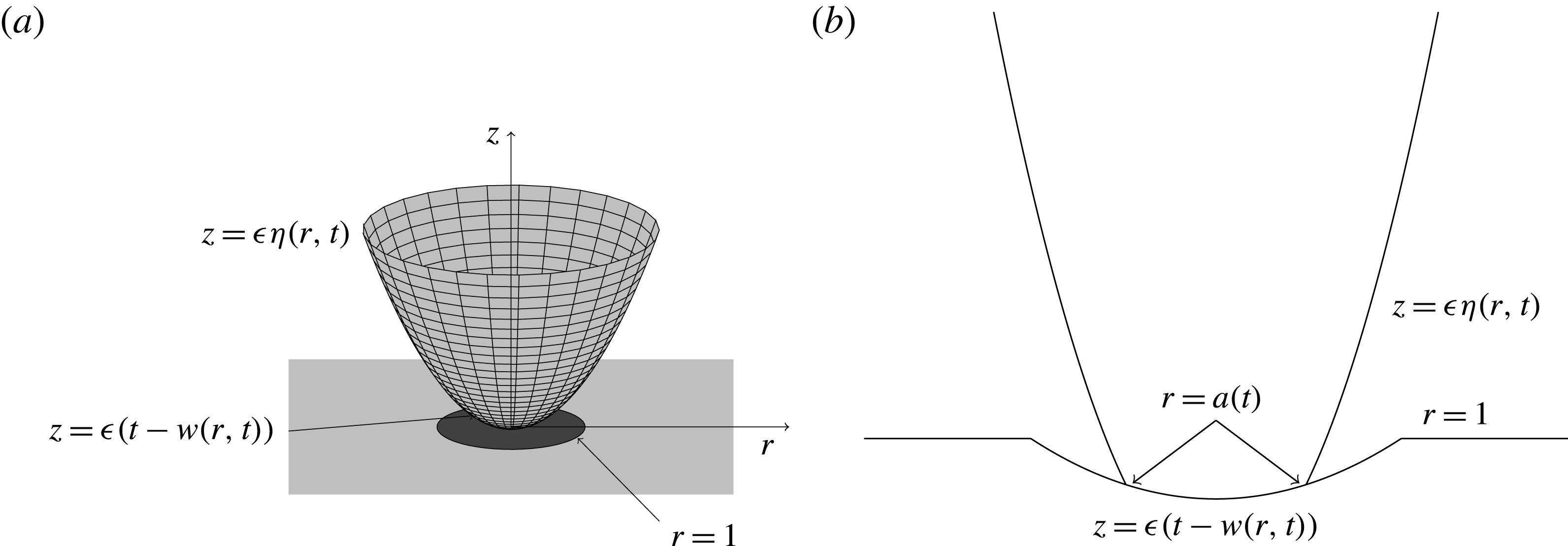
, at a single point which is taken as the origin of the coordinate system (see figure 2). The initial surface of the drop is described by the equation
 $$\begin{eqnarray}z=\frac{\unicode[STIX]{x1D716}}{2}(r^{2}+z^{2}).\end{eqnarray}$$
For mathematical convenience we chose a frame of reference where the droplet is initially at rest and the substrate hits the liquid drop at unit speed from below. The position of the moving substrate is given by
 $$\begin{eqnarray}z=\unicode[STIX]{x1D716}(t-w(r,t)),\end{eqnarray}$$
where
 $w(r,t)$
is the deflection of the elastic part,
 $r<1$
, of the substrate, and
 $w(r,t)=0$
elsewhere. The deflection
 $w(r,t)$
is taken to be positive in the negative
 $z$
-direction.
The flow in the droplet is described by the velocity potential
 $\unicode[STIX]{x1D711}(r,z,t)$
. The potential satisfies Laplace’s equation in the flow region,
 $\unicode[STIX]{x1D6FA}(t,\unicode[STIX]{x1D716})$
, and is subject to the kinematic boundary condition,
 $$\begin{eqnarray}\unicode[STIX]{x1D711}_{z}=\unicode[STIX]{x1D716}\unicode[STIX]{x1D702}_{r}\unicode[STIX]{x1D711}_{r}+\unicode[STIX]{x1D702}_{t},\end{eqnarray}$$
on the free surface of the drop,
 $z=\unicode[STIX]{x1D716}\unicode[STIX]{x1D702}(r,t)$
, where
 $\unicode[STIX]{x1D702}(r,0)=(1/2)r^{2}+O(\unicode[STIX]{x1D716})$
and
 $r=O(1)$
, and the body boundary condition
 $$\begin{eqnarray}\unicode[STIX]{x1D711}_{z}=1-w_{t}-\unicode[STIX]{x1D716}w_{r}\unicode[STIX]{x1D711}_{r},\end{eqnarray}$$
on the moving substrate (2.3), in the wetted region where
 $r<a(t,\unicode[STIX]{x1D716})$
. This wetted region is unknown in advance and should be found as part of the solution; the unknown function
 $a(t,\unicode[STIX]{x1D716})$
gives the radius of the contact region (neglecting the thin jet discussed later). The dynamic boundary condition on the free surface of the impacted drop is
 $$\begin{eqnarray}p(r,\unicode[STIX]{x1D716}\unicode[STIX]{x1D702}(r,t),t)=0,\end{eqnarray}$$
where the hydrodynamic pressure
 $p(r,z,t)$
is given by the Bernoulli equation,
 $$\begin{eqnarray}p(r,z,t)=-\unicode[STIX]{x1D711}_{t}-{\textstyle \frac{1}{2}}\unicode[STIX]{x1D716}|\unicode[STIX]{x1D735}\unicode[STIX]{x1D711}|^{2}.\end{eqnarray}$$
The plate deflection
 $w(r,t)$
is taken to be described by the thin plate theory:
 $$\begin{eqnarray}\unicode[STIX]{x1D6FC}w_{tt}+\unicode[STIX]{x1D6FD}\unicode[STIX]{x1D6FB}^{4}w=p(r,\unicode[STIX]{x1D716}(t-w(r,t)),t),\quad (r\leqslant 1),\end{eqnarray}$$
where
 $$\begin{eqnarray}\unicode[STIX]{x1D6FC}=\frac{\unicode[STIX]{x1D70C}_{p}h}{\unicode[STIX]{x1D70C}L},\quad \unicode[STIX]{x1D6FD}=\frac{Eh^{3}\unicode[STIX]{x1D716}^{2}}{12(1-\unicode[STIX]{x1D708}^{2})\unicode[STIX]{x1D70C}V^{2}L^{3}},\end{eqnarray}$$
 $\unicode[STIX]{x1D70C}_{p}$
is the density of the elastic plate,
 $h$
is the plate thickness,
 $E$
is the Young modulus of the plate material, and
 $\unicode[STIX]{x1D708}$
is the Poisson ratio. The parameter
 $\unicode[STIX]{x1D6FC}$
indicates the importance of the structural mass per unit area of the plate,
 $\unicode[STIX]{x1D70C}_{p}h$
, compared to the added mass of the liquid per unit area, which is of the order of
 $O(\unicode[STIX]{x1D70C}L)$
. The parameter
 $\unicode[STIX]{x1D6FD}$
can be considered as the dynamic rigidity of the plate. This parameter depends on the elastic characteristics of the plate, speed of impact and the size of the drop. We assume that both
 $\unicode[STIX]{x1D6FC}$
and
 $\unicode[STIX]{x1D6FD}$
are of order
 $O(1)$
in the present analysis, which guarantees strong coupling between hydrodynamic loads and the plate deflection. Outside the wetted region,
 $r>a(t,\unicode[STIX]{x1D716})$
, the right-hand side in (2.8) is zero. We assume that the elastic plate is simply supported at
 $r=1$
and flat initially. Then the plate equation (2.8) is to be solved subject to the initial and boundary conditions
 $$\begin{eqnarray}\displaystyle w=0,\quad w_{rr}+\frac{\unicode[STIX]{x1D708}}{r}w_{r}=0,\quad (r=1), & & \displaystyle\end{eqnarray}$$
 $$\begin{eqnarray}\displaystyle w(r,0)=0,\quad w_{t}(r,0)=0\quad (r\leqslant 1). & & \displaystyle\end{eqnarray}$$
The formulation of the fully coupled problem is completed by the initial conditions
 $$\begin{eqnarray}\displaystyle & \displaystyle \unicode[STIX]{x1D711}(r,z,0)=0, & \displaystyle\end{eqnarray}$$
 $$\begin{eqnarray}\displaystyle & \displaystyle a(0,\unicode[STIX]{x1D716})=0, & \displaystyle\end{eqnarray}$$
 $$\begin{eqnarray}\displaystyle & \displaystyle \unicode[STIX]{x1D702}(r,0)={\textstyle \frac{1}{2}}r^{2}+O(\unicode[STIX]{x1D716}), & \displaystyle\end{eqnarray}$$
where
 $r=O(1)$
and
 $z=O(1)$
. The pressure
 $p(r,z,t)$
in (2.6) and (2.7) does not account for ambient pressure, hydrostatic pressure and the pressure due to surface tension effects. The hydrostatic pressure is of the order of
 $\unicode[STIX]{x1D70C}gR$
, which is much smaller than the dynamic pressure scale
 $\unicode[STIX]{x1D70C}V^{2}R/L$
if
 $\unicode[STIX]{x1D716}(gR/V^{2})\ll 1$
. The surface tension can be neglected at leading order if the inverse Weber number
 $We^{-1}=\unicode[STIX]{x1D70E}/(\unicode[STIX]{x1D70C}V^{2}R)\ll 1$
, where
 $\unicode[STIX]{x1D70E}$
is the coefficient of surface tension of the liquid. For a water droplet of density
 $\unicode[STIX]{x1D70C}=1000~\text{kg}~\text{m}^{-3}$
, surface tension
 $\unicode[STIX]{x1D70E}=7.2\times 10^{-2}~\text{N}~\text{m}^{-1}$
and radius
 $R=5\times 10^{-3}~\text{m}$
, with
 $g=9.81~\text{m}~\text{s}^{-2}$
impacting an elastic circular disk of radius
 $L=1\times 10^{-3}~\text{m}$
at velocity
 $V=1~\text{m}~\text{s}^{-1}$
, we have
 $\unicode[STIX]{x1D70E}/(\unicode[STIX]{x1D70C}V^{2}R)<0.0144$
and
 $\unicode[STIX]{x1D716}(gR/V^{2})<10^{-2}$
. Hence we neglect surface tension and gravity, as both provide smaller contributions to the hydrodynamic pressure compared to that from inertia.
The problem formulated above is strongly coupled. The plate deflection depends on the hydrodynamic loads through the right-hand side of (2.8), and both the hydrodynamic pressure (2.7) and the flow in the liquid droplet depend on the elastic deflection of the plate through the body boundary condition (2.5). The flow region,
 $\unicode[STIX]{x1D6FA}(\unicode[STIX]{x1D716},t)$
, and the wetted area of the plate,
 $r<a(t,\unicode[STIX]{x1D716})$
, are unknown in advance and should be determined along with the hydrodynamic and structural characteristics of the problem.
The problem (2.2)–(2.14) can be simplified during the early stage of impact. The approximate solution can be obtained by asymptotic methods as
 $\unicode[STIX]{x1D716}\rightarrow 0$
. Equations (2.2)–(2.3) show that the flow region can be approximated by the upper half-space,
 $z>0$
, to leading order, and the boundary conditions (2.4)–(2.6) can be linearised and imposed on the plane
 $z=0$
. In addition, the linearised dynamic condition (2.6) can be integrated in time using the initial conditions. Below we keep the original notations of the unknown functions for their leading-order terms. At leading order, the hydrodynamic part of the problem reads
 $$\begin{eqnarray}\displaystyle & \displaystyle \unicode[STIX]{x1D6FB}^{2}\unicode[STIX]{x1D711}=0,\quad (z>0), & \displaystyle\end{eqnarray}$$
 $$\begin{eqnarray}\displaystyle & \displaystyle \unicode[STIX]{x1D711}=0,\quad (z=0,r>a(t)), & \displaystyle\end{eqnarray}$$
 $$\begin{eqnarray}\displaystyle & \displaystyle \unicode[STIX]{x1D711}_{z}=1-w_{t}(r,t),\quad (z=0,r\leqslant a(t)), & \displaystyle\end{eqnarray}$$
 $$\begin{eqnarray}\displaystyle & \displaystyle \unicode[STIX]{x1D711}\rightarrow 0,\quad (r^{2}+z^{2}\rightarrow \infty ), & \displaystyle\end{eqnarray}$$
where
 $w(r,t)=0$
for
 $r>1$
. The hydrodynamic pressure is given by the linearised Bernoulli equation,
 $p(r,z,t)=-\unicode[STIX]{x1D711}_{t}(r,z,t)$
. The plate equation (2.8) at leading order then becomes
 $$\begin{eqnarray}\displaystyle \frac{\unicode[STIX]{x2202}}{\unicode[STIX]{x2202}t}(\unicode[STIX]{x1D6FC}w_{t}(r,t)+\unicode[STIX]{x1D711}(r,0,t))+\unicode[STIX]{x1D6FD}\unicode[STIX]{x1D6FB}^{4}w=0,\quad (r<1). & & \displaystyle\end{eqnarray}$$
Equation (2.19) is solved subject to the boundary conditions (2.10) and initial conditions (2.11). The shape of the liquid free surface,
 $z=\unicode[STIX]{x1D716}\unicode[STIX]{x1D702}(r,t)$
, is provided at leading order by
 $\unicode[STIX]{x1D702}_{t}(r,t)=\unicode[STIX]{x1D711}_{z}(r,0,t)$
, where
 $r>a(t)$
, which follows from the kinematic condition (2.4). Note that
 $\unicode[STIX]{x1D702}(r,0)\rightarrow r^{2}/2$
as
 $\unicode[STIX]{x1D716}\rightarrow 0$
. The equations of flow, (2.15)–(2.18), and the equation of the plate deflection (2.19) at leading order are linear but crucially still coupled.
The radius of the contact region between the liquid and substrate,
 $r<a(t)$
, is determined by using the condition that the vertical coordinate of the free surface,
 $z=\unicode[STIX]{x1D716}\unicode[STIX]{x1D702}(a(t),t)$
at the contact line
 $r=a(t)$
, and the vertical coordinate of the elastic substrate (2.3) are equal, namely
 $$\begin{eqnarray}\unicode[STIX]{x1D702}(a(t),t)=t-w(a(t),t).\end{eqnarray}$$
Condition (2.20) is known as the Wagner condition (Wagner Reference Wagner1932). This condition assumes that the spray jet formed at the periphery of the contact region is thin and can be neglected at leading order as
 $\unicode[STIX]{x1D716}\rightarrow 0$
. The Wagner condition makes the leading-order problem nonlinear. As in Korobkin (Reference Korobkin1982), we can reduce the Wagner condition (2.20) to
 $$\begin{eqnarray}\int _{0}^{\unicode[STIX]{x03C0}/2}\sin (\unicode[STIX]{x1D703})F(a(t)\sin (\unicode[STIX]{x1D703}),t)\,\text{d}\unicode[STIX]{x1D703}=0,\end{eqnarray}$$
where
 $F(r,t)=t-w(r,t)-r^{2}/2$
is the distance between the initial position of the liquid free surface and the current position of the impacting elastic substrate. See Korobkin (Reference Korobkin1996) and Korobkin & Scolan (Reference Korobkin and Scolan2006) for full details of this approach for related problems. Note that the radius of the contact region
 $a(t)$
depends strongly on the plate deflection
 $w(r,t)$
.
The hydrodynamic problem (2.15)–(2.18) is solved by the method of dual integral equations (Sneddon Reference Sneddon1966) and the plate deflection is obtained by the method of normal modes (Korobkin Reference Korobkin1998; Scolan Reference Scolan2004) applied to the structural problem (2.19), (2.10), (2.11), where the radius
 $a(t)$
of the contact region is determined by equation (2.21).
(a) A sketch of the problem away from the contact region. The light grey paraboloid shows the liquid free surface
 $z=\unicode[STIX]{x1D716}\unicode[STIX]{x1D702}(r,t)$
, the dark grey circle is the elastic plate with deformation
 $z=\unicode[STIX]{x1D716}(t-w(r,t))$
and the light grey square region indicates the infinite rigid substrate for the elastic plate. (b) A side-on view of the impact situation for time
 $t>0$
with plate deflection
 $w(r,t)$
shown. The substrate moves upwards towards the droplet, which is initially at rest, at a unit speed in the non-dimensional variables.

3 Coupled problem of hydroelastic impact
The formulated problem (2.10)–(2.11), (2.15)–(2.21) is coupled. The hydrodynamic part of the problem (2.15) subject to (2.16)–(2.18), and the structural part of the problem (2.19), subject to (2.10)–(2.11) should be solved simultaneously, together with the Wagner condition (2.21) for the unknown radius of the contact region,
 $a(t)$
.
3.1 Structural problem
It is convenient to introduce a new unknown function,
 $$\begin{eqnarray}q(r,t)=-\frac{1}{\unicode[STIX]{x1D6FD}}(\unicode[STIX]{x1D6FC}w_{t}(r,t)+\unicode[STIX]{x1D711}(r,0,t)),\end{eqnarray}$$
where
 $0\leqslant r<1$
, and to rewrite equation (2.19) as
 $$\begin{eqnarray}\displaystyle & \displaystyle q_{t}=\unicode[STIX]{x1D6FB}^{4}w, & \displaystyle\end{eqnarray}$$
 $$\begin{eqnarray}\displaystyle & \displaystyle \unicode[STIX]{x1D6FC}w_{t}+\unicode[STIX]{x1D711}(r,0,t)=-\unicode[STIX]{x1D6FD}q(r,t). & \displaystyle\end{eqnarray}$$
Here
 $\unicode[STIX]{x1D711}(r,0,t)=0$
, where
 $a(t)\leqslant r<1$
, during the early stage when the elastic plate is only partly in contact with the liquid,
 $a(t)<1$
. Within the method of normal modes, the deflection
 $w(r,t)$
and auxiliary function
 $q(r,t)$
are sought in the forms
 $$\begin{eqnarray}\displaystyle & \displaystyle w(r,t)=\mathop{\sum }_{n=1}^{\infty }A_{n}(t)w_{n}(r), & \displaystyle\end{eqnarray}$$
 $$\begin{eqnarray}\displaystyle & \displaystyle q(r,t)=\mathop{\sum }_{n=1}^{\infty }k_{n}^{4}q_{n}(t)w_{n}(r), & \displaystyle\end{eqnarray}$$
where
 $A_{n}(t)$
and
 $q_{n}(t)$
are the coefficients to be determined. The functions
 $w_{n}(r)$
are the non-trivial bounded solutions to the homogeneous boundary value problem
 $$\begin{eqnarray}\displaystyle \unicode[STIX]{x1D6FB}^{4}w_{n}=k_{n}^{4}w_{n},\quad r<1, & & \displaystyle\end{eqnarray}$$
 $$\begin{eqnarray}\displaystyle w_{n}(1)=0,\quad w_{n}^{\prime \prime }(1)+\unicode[STIX]{x1D708}w_{n}^{\prime }(1)=0, & & \displaystyle\end{eqnarray}$$
and
 $k_{n}$
are the corresponding eigenvalues. The functions
 $w_{n}(r)$
describe the axisymmetric shapes of free vibrations of a circular simply supported plate with frequencies proportional to
 $k_{n}^{2}$
(Leissa Reference Leissa1969). The solutions have the form
 $$\begin{eqnarray}w_{n}(r)=\text{J}_{0}(k_{n}r)-\frac{\text{J}_{0}(k_{n})}{\text{I}_{0}(k_{n})}\text{I}_{0}(k_{n}r),\end{eqnarray}$$
where
 $k_{n}$
are the solutions of the equation
 $$\begin{eqnarray}\frac{\text{J}_{1}(k_{n})}{\text{J}_{0}(k_{n})}+\frac{\text{I}_{1}(k_{n})}{\text{I}_{0}(k_{n})}=\frac{2k_{n}}{1-\unicode[STIX]{x1D708}},\end{eqnarray}$$
with
 $n\geqslant 1$
and
 $k_{n+1}>k_{n}$
. Here
 $\text{J}_{n}(r)$
and
 $\text{I}_{n}(r)$
are the Bessel functions of the first kind and modified Bessel functions of the first kind of order
 $n$
respectively. The functions (3.8) are orthogonal but not normalised:
 $$\begin{eqnarray}\int _{0}^{1}w_{n}(r)w_{m}(r)r\,\text{d}r=U_{n}\unicode[STIX]{x1D6FF}_{nm},\end{eqnarray}$$
where
 $U_{n}$
are given in appendix A, and where
 $\unicode[STIX]{x1D6FF}_{nm}=0$
for
 $n\neq m$
and
 $\unicode[STIX]{x1D6FF}_{nn}=1$
.
3.2 Coupled problem
The equations (3.3), (3.4) and (3.5) together with initial conditions (2.11) provide the system of ordinary differential equations for the vector
 $\boldsymbol{q}(t)=\{q_{1}(t),q_{2}(t),\ldots \}$
,
 $$\begin{eqnarray}\dot{\boldsymbol{q}}=\boldsymbol{A}(t),\quad \boldsymbol{q}(0)=0,\end{eqnarray}$$
where
 $\boldsymbol{A}(t)=\{A_{1}(t),A_{2}(t),\ldots \}$
is the vector of coefficients in the series (3.4), and overdot stands for time derivative. The boundary problem (2.15)–(2.18) for the velocity potential
 $\unicode[STIX]{x1D711}(r,z,t)$
and the series for the plate deflection (3.4) lead to the following decomposition of the potential:
 $$\begin{eqnarray}\unicode[STIX]{x1D711}(r,z,t)=\unicode[STIX]{x1D711}_{0}(r,z,a)-\mathop{\sum }_{n=1}^{\infty }{\dot{A}}_{n}(t)\unicode[STIX]{x1D711}_{n}(r,z,a).\end{eqnarray}$$
Here
 $\unicode[STIX]{x1D711}_{0}(r,z,a)$
is the potential of the flow caused by the impact of the rigid circular disk of radius
 $a$
with the condition on the disc,
 $\unicode[STIX]{x1D711}_{0,z}(r,0,a)=1$
. The potentials
 $\unicode[STIX]{x1D711}_{n}(r,z,a)$
satisfy (2.15) and (2.18), with the condition (2.17) becoming
 $\unicode[STIX]{x1D711}_{n,z}(r,0,a)=w_{n}(r)$
, for
 $r<a$
. Substituting (3.12) and (3.4) into the second equation of (3.3), multiplying both sides of this equation by
 $w_{m}(r)r$
, and integrating in
 $r$
from
 $0$
to
 $1$
, we find
 $$\begin{eqnarray}\displaystyle & & \displaystyle \unicode[STIX]{x1D6FC}{\dot{A}}_{m}U_{m}+\int _{0}^{a}\unicode[STIX]{x1D711}_{0}(r,0,a)w_{m}(r)r\,\text{d}r-\mathop{\sum }_{n=0}^{\infty }{\dot{A}}_{n}(t)\int _{0}^{a}\unicode[STIX]{x1D711}_{n}(r,0,a)w_{m}(r)r\,\text{d}r\nonumber\\ \displaystyle & & \displaystyle \quad =-\unicode[STIX]{x1D6FD}k_{m}^{4}q_{m}(t)U_{m},\end{eqnarray}$$
which can be written more concisely in vector form as
 $$\begin{eqnarray}\dot{\boldsymbol{A}}=-(\unicode[STIX]{x1D726}+\unicode[STIX]{x1D652}(a))^{-1}(\unicode[STIX]{x1D655}\boldsymbol{q}-\boldsymbol{g}(a)),\quad \boldsymbol{A}(0)=0.\end{eqnarray}$$
Here
 $\unicode[STIX]{x1D726}=\text{diag}\{\unicode[STIX]{x1D6FC}U_{1},\unicode[STIX]{x1D6FC}U_{2},\ldots \}$
and
 $\unicode[STIX]{x1D655}=\text{diag}\{\unicode[STIX]{x1D6FD}k_{1}^{4}U_{1},\unicode[STIX]{x1D6FD}k_{2}^{4}U_{2},\ldots \}$
are diagonal matrices. The elements of the vector
 $\boldsymbol{g}(a)$
are
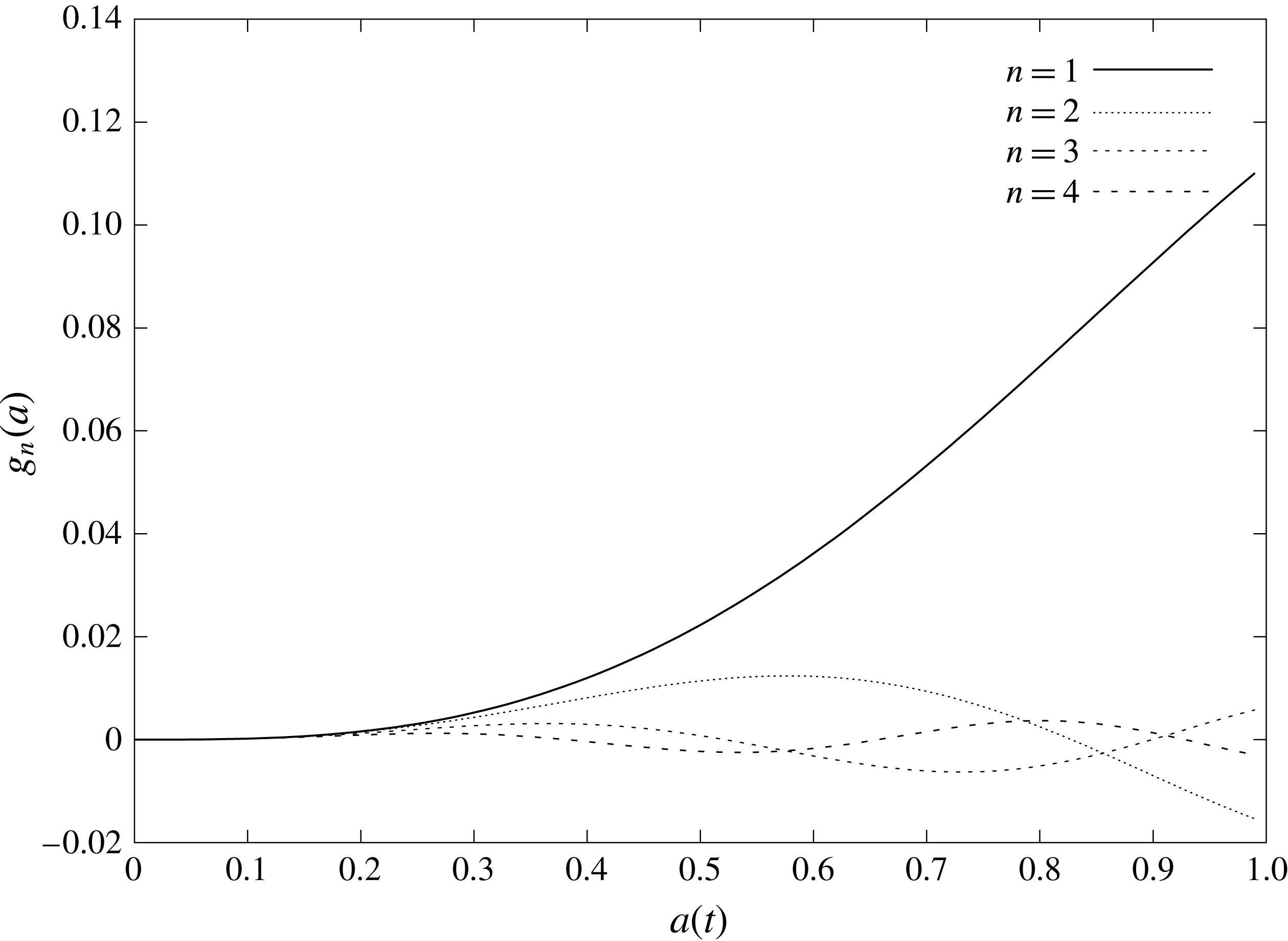
 $$\begin{eqnarray}g_{n}(a)=-\int _{0}^{a}\unicode[STIX]{x1D711}_{0}(r,0,a)w_{n}(r)r\,\text{d}r,\end{eqnarray}$$
and the symmetric added mass matrix
 $\unicode[STIX]{x1D652}(a)$
has the elements
 $$\begin{eqnarray}\unicode[STIX]{x1D61E}_{nm}(a)=-\int _{0}^{a}\unicode[STIX]{x1D711}_{n}(r,0,a)w_{m}(r)r\,\text{d}r.\end{eqnarray}$$
The system of ordinary differential equations (3.11) and (3.14) is valid for
 $a\leqslant 1$
. For the later stages, when
 $a(t)>1$
and the elastic plate is completely wetted, we should change the upper limits in (3.15) and (3.16) to
 $1$
and set
 $w_{n}(r)=0$
, where
 $r>1$
in the boundary conditions for the potentials
 $\unicode[STIX]{x1D711}_{n}(r,z,a)$
. The coefficients in (3.14) depend on the radius of the wetted area,
 $a(t)$
, which is defined by equation (2.21). Substituting for
 $F(r,t)$
and the series (3.4) in (2.21), we find
 $$\begin{eqnarray}t-\frac{1}{2}a^{2}(t)\int _{0}^{\unicode[STIX]{x03C0}/2}\sin ^{3}(\unicode[STIX]{x1D703})\,\text{d}\unicode[STIX]{x1D703}-\mathop{\sum }_{n=1}^{\infty }A_{n}(t)\int _{0}^{\unicode[STIX]{x03C0}/2}\sin (\unicode[STIX]{x1D703})w_{n}(a\sin (\unicode[STIX]{x1D703}))\,\text{d}\unicode[STIX]{x1D703}=0,\end{eqnarray}$$
and then
 $$\begin{eqnarray}a^{2}(t)=3t-3\boldsymbol{A}(t)\boldsymbol{\cdot }\boldsymbol{Q}(a),\end{eqnarray}$$
where
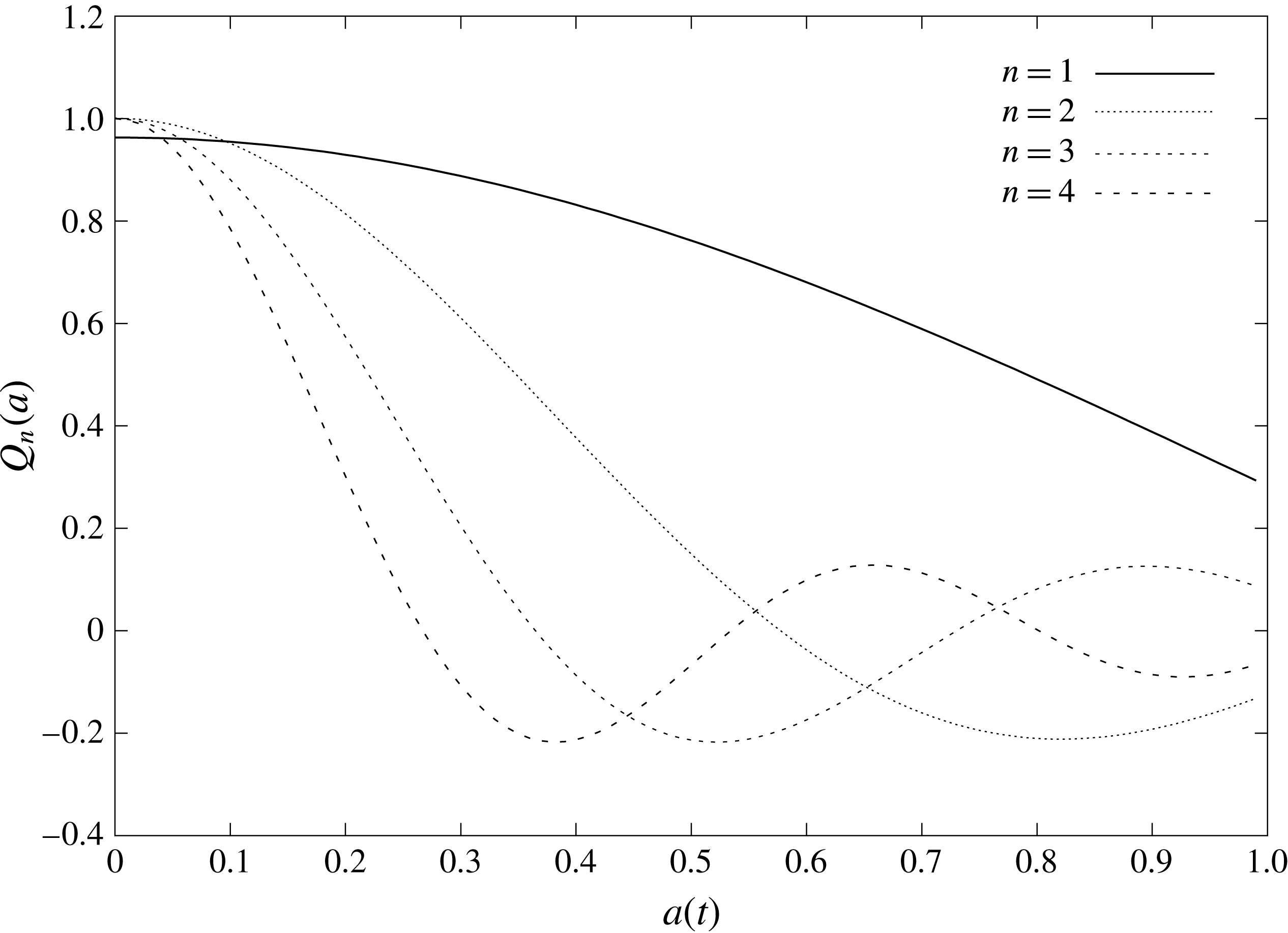
 $$\begin{eqnarray}Q_{n}(a)=\int _{0}^{\unicode[STIX]{x03C0}/2}\sin (\unicode[STIX]{x1D703})w_{n}(a\sin (\unicode[STIX]{x1D703}))\,\text{d}\unicode[STIX]{x1D703}=\frac{1}{a}\int _{0}^{a}\frac{\unicode[STIX]{x1D70C}w_{n}(\unicode[STIX]{x1D70C})\,\text{d}\unicode[STIX]{x1D70C}}{\sqrt{a^{2}-\unicode[STIX]{x1D70C}^{2}}}.\end{eqnarray}$$
Note that
 $w_{n}(a\sin (\unicode[STIX]{x1D703}))\equiv 0$
, where
 $a\sin (\unicode[STIX]{x1D703})>1$
. The system (3.11), (3.14) and (3.18) can be solved numerically once the integrals (3.15), (3.16) and (3.19) are known functions of
 $a$
. The functions
 $Q_{n}(a)$
and
 $g_{n}(a)$
are evaluated in appendices B and C, respectively.
3.3 Hydrodynamic problem
The hydrodynamic problem (2.15)–(2.18), together with the decomposition (3.12), leads to two mixed boundary value problems. The rigid part of the decomposition (3.12) becomes
 $$\begin{eqnarray}\displaystyle & \displaystyle \unicode[STIX]{x1D6FB}^{2}\unicode[STIX]{x1D711}_{0}=0,\quad (z>0), & \displaystyle\end{eqnarray}$$
 $$\begin{eqnarray}\displaystyle & \displaystyle \unicode[STIX]{x1D711}_{0}=0,\quad (z=0,r>a(t)), & \displaystyle\end{eqnarray}$$
 $$\begin{eqnarray}\displaystyle & \displaystyle \unicode[STIX]{x1D711}_{0,z}=1,\quad (z=0,r\leqslant a(t)), & \displaystyle\end{eqnarray}$$
 $$\begin{eqnarray}\displaystyle & \displaystyle \unicode[STIX]{x1D711}_{0}\rightarrow 0,\quad (r^{2}+z^{2}\rightarrow \infty ), & \displaystyle\end{eqnarray}$$
whilst the elastic part of the decomposition requires
 $$\begin{eqnarray}\displaystyle & \displaystyle \unicode[STIX]{x1D6FB}^{2}\unicode[STIX]{x1D711}_{n}=0,\quad (z>0), & \displaystyle\end{eqnarray}$$
 $$\begin{eqnarray}\displaystyle & \displaystyle \unicode[STIX]{x1D711}_{n}=0,\quad (z=0,r>a(t)), & \displaystyle\end{eqnarray}$$
 $$\begin{eqnarray}\displaystyle & \displaystyle \unicode[STIX]{x1D711}_{n,z}=w_{n}(r),\quad (z=0,r\leqslant a(t)), & \displaystyle\end{eqnarray}$$
 $$\begin{eqnarray}\displaystyle & \displaystyle \unicode[STIX]{x1D711}_{n}\rightarrow 0,\quad (r^{2}+z^{2}\rightarrow \infty ), & \displaystyle\end{eqnarray}$$
where
 $n\geqslant 1$
.
These mixed boundary value problems are solved through the use of Hankel transformations. Equations (3.20) and (3.23) give
 $$\begin{eqnarray}\unicode[STIX]{x1D711}_{0}(r,z,a)=\int _{0}^{\infty }G_{0}(\unicode[STIX]{x1D706},a)e^{-\unicode[STIX]{x1D706}z}\text{J}_{0}(\unicode[STIX]{x1D706}r)\,\text{d}\unicode[STIX]{x1D706},\end{eqnarray}$$
where
 $G_{0}(\unicode[STIX]{x1D706},a)$
is a new unknown function. Substituting (3.28) in the boundary conditions (3.21) and (3.22) gives us the dual integral equations
 $$\begin{eqnarray}\displaystyle & \displaystyle \int _{0}^{\infty }G_{0}(\unicode[STIX]{x1D706},a)\text{J}_{0}(\unicode[STIX]{x1D706}r)\,\text{d}\unicode[STIX]{x1D706}=0,\quad r>a & \displaystyle\end{eqnarray}$$
 $$\begin{eqnarray}\displaystyle & \displaystyle \int _{0}^{\infty }G_{0}(\unicode[STIX]{x1D706},a)\unicode[STIX]{x1D706}\text{J}_{0}(\unicode[STIX]{x1D706}r)\,\text{d}\unicode[STIX]{x1D706}=-1,\quad r\leqslant a. & \displaystyle\end{eqnarray}$$
These equations were solved by Sneddon (Reference Sneddon1966), yielding
 $$\begin{eqnarray}G_{0}(\unicode[STIX]{x1D706},a)=-\sqrt{\frac{2\unicode[STIX]{x1D706}}{\unicode[STIX]{x03C0}}}\int _{0}^{a}\sqrt{x}\text{J}_{1/2}(x\unicode[STIX]{x1D706})\,\text{d}x\int _{0}^{x}\frac{\unicode[STIX]{x1D70C}\,\text{d}\unicode[STIX]{x1D70C}}{\sqrt{x^{2}-\unicode[STIX]{x1D70C}^{2}}}.\end{eqnarray}$$
Equations (3.31) and (3.28) provide
 $$\begin{eqnarray}\unicode[STIX]{x1D711}_{0}(r,0,a)=-\sqrt{\frac{2}{\unicode[STIX]{x03C0}}}\int _{0}^{a}\sqrt{x}\,\text{d}x\int _{0}^{x}\frac{\unicode[STIX]{x1D70C}\,\text{d}\unicode[STIX]{x1D70C}}{\sqrt{x^{2}-\unicode[STIX]{x1D70C}^{2}}}\int _{0}^{\infty }\sqrt{\unicode[STIX]{x1D706}}\text{J}_{0}(\unicode[STIX]{x1D706}r)\text{J}_{1/2}(\unicode[STIX]{x1D706}x)\,\text{d}\unicode[STIX]{x1D706}.\end{eqnarray}$$
This can be integrated directly (with the
 $\unicode[STIX]{x1D706}$
integral given by 6.575.1 of Gradshteyn & Ryzhik (Reference Gradshteyn and Ryzhik2007)) to give an explicit expression for the rigid velocity potential,
 $$\begin{eqnarray}\displaystyle \unicode[STIX]{x1D711}_{0}(r,0,a)=-\frac{2}{\unicode[STIX]{x03C0}}\sqrt{a^{2}-r^{2}},\quad (r\leqslant a). & & \displaystyle\end{eqnarray}$$
The elastic part of the problem (3.24)–(3.27) is solved using the same method. The elastic terms of the velocity potential,
 $\unicode[STIX]{x1D711}_{n}(r,0,a)$
, are given by
 $$\begin{eqnarray}\unicode[STIX]{x1D711}_{n}(r,0,a)=-\frac{2}{\unicode[STIX]{x03C0}}\int _{r}^{a}\frac{\text{d}x}{\sqrt{x^{2}-r^{2}}}\int _{0}^{x}\frac{\unicode[STIX]{x1D70C}w_{n}(\unicode[STIX]{x1D70C})\,\text{d}\unicode[STIX]{x1D70C}}{\sqrt{x^{2}-\unicode[STIX]{x1D70C}^{2}}}.\end{eqnarray}$$
By using (3.19) we can express (3.34) as
 $$\begin{eqnarray}\unicode[STIX]{x1D711}_{n}(r,0,a)=-\frac{2}{\unicode[STIX]{x03C0}}\int _{r}^{a}\frac{xQ_{n}(x)\,\text{d}x}{\sqrt{x^{2}-r^{2}}}=-\unicode[STIX]{x1D6F7}_{n}(r,a),\end{eqnarray}$$
and (3.12) as
 $$\begin{eqnarray}\displaystyle \unicode[STIX]{x1D711}(r,0,a)=-\frac{2}{\unicode[STIX]{x03C0}}\sqrt{a^{2}-r^{2}}+\mathop{\sum }_{n=1}^{\infty }{\dot{A}}_{n}(t)\unicode[STIX]{x1D6F7}_{n}(r,a),\quad (r\leqslant a). & & \displaystyle\end{eqnarray}$$
The added-mass elements (3.16) then become
 $$\begin{eqnarray}\displaystyle \unicode[STIX]{x1D61E}_{nm}=\frac{2}{\unicode[STIX]{x03C0}}\int _{0}^{a}\left(\int _{r}^{a}\frac{xQ_{n}(x)\,\text{d}x}{\sqrt{x^{2}-r^{2}}}\right)w_{m}(r)\,\text{d}r=\frac{2}{\unicode[STIX]{x03C0}}\int _{0}^{a}x^{2}Q_{n}(x)Q_{m}(x)\,\text{d}x. & & \displaystyle\end{eqnarray}$$
The integrals (3.37) are evaluated analytically in appendix D. Integrating in (3.35) by parts, we obtain
 $$\begin{eqnarray}\unicode[STIX]{x1D6F7}_{n}(r,a)=\frac{2}{\unicode[STIX]{x03C0}}Q_{n}(a)\sqrt{a^{2}-r^{2}}-\frac{2}{\unicode[STIX]{x03C0}}\int _{r}^{a}\sqrt{x^{2}-r^{2}}Q_{n}^{\prime }(x)\,\text{d}x,\end{eqnarray}$$
where
 $Q_{n}(a)$
is given by (3.19).
Equations (3.38) and (3.36) provide the behaviour of the velocity potential close to the contact line as
 $r\rightarrow a(t)$
,
 $$\begin{eqnarray}\unicode[STIX]{x1D711}(r,0,t)=B(t)\sqrt{a(t)-r}+O((a-r)^{3/2}),\end{eqnarray}$$
where
 $$\begin{eqnarray}B(t)=\frac{2}{\unicode[STIX]{x03C0}}\sqrt{2a}\left(\mathop{\sum }_{n=1}^{\infty }{\dot{A}}_{n}(t)Q_{n}(a)-1\right).\end{eqnarray}$$
Therefore the Wagner model predicts a square-root singularity in the radial velocity of the flow in the main region,
 $(\unicode[STIX]{x2202}\unicode[STIX]{x1D711}/\unicode[STIX]{x2202}r)(r,0,t)$
, and in the hydrodynamic pressure,
 $p(r,0,t)=-\unicode[STIX]{x2202}\unicode[STIX]{x1D711}/\unicode[STIX]{x2202}t$
, at the contact line as
 $r\rightarrow a(t)$
. The coefficient of this singularity,
 $B(t)$
, depends on the plate deflection and is calculated as part of the solution in the main flow region. The Wagner model is not valid at the periphery of the contact region. In Wagner-type problems, this singularity is resolved by introducing an inner region, the so-called jet-root region, around the contact line (Howison et al.
Reference Howison, Ockendon and Wilson1991). This locally resolves the singularity by the presence of a thin jet running along the substrate. This local inner solution is discussed below.
4 Jet-root and jet regions
The dynamics of the jet and its dependence on elastic oscillations of the plate play a key role in potential splashing of the droplet. We distinguish the jet-root region, which is in a small vicinity of the contact line and is characterised by large velocities and pressures, and the jet itself. The equations governing the flows in both the jet-root region and the jet region are derived by using stretched variables. For the jet-root region
 $r=a(t)+\unicode[STIX]{x1D716}^{2}X$
,
 $z=\unicode[STIX]{x1D716}(t-w(a,t))+\unicode[STIX]{x1D716}^{2}Z$
and
 $\unicode[STIX]{x1D711}=\unicode[STIX]{x1D716}(\unicode[STIX]{x1D719}(X,Z,t)+{\dot{a}}X)$
are used in the limit
 $\unicode[STIX]{x1D716}\rightarrow 0$
. Howison et al. (Reference Howison, Ockendon and Wilson1991) and Oliver (Reference Oliver2002) contain full details of the case for impact with a rigid substrate. We do not provide details of the asymptotic analysis here, and instead just highlight how the elastic substrate affects the solution.
In the jet-root region the singularity found in the pressure above is resolved by considering a locally two-dimensional flow problem around the contact line
 $r=a(t)$
subject to the far-field condition which follows from (3.39) as
 $X^{2}+Y^{2}\rightarrow \infty$
. Locally the jet-root flow is the same as in the problem of a rapid rigid body impact onto a water free surface. The latter problem was studied by Oliver (Reference Oliver2002). In our situation the key difference is in the
 $B(t)$
term of the far-field condition, which contains additional elastic terms: see equation (3.40). The important results are the initial thickness of the jet,
 $$\begin{eqnarray}H_{j}(t)=\frac{\unicode[STIX]{x03C0}}{16}\frac{B^{2}}{{\dot{a}}^{2}},\end{eqnarray}$$
and the velocity of fluid entering the jet
 $2{\dot{a}}(t)$
, in the static frame of reference.
Note that without the elastic deflection of the plate,
 $A_{j}(t)=0$
in (3.18) and (3.40), the Wagner condition requires
 $a(t)=\sqrt{3t}$
, giving
 $B=-2\sqrt{2a}/\unicode[STIX]{x03C0}$
in the non-dimensional variables. The jet thickness (4.1) is then given by
 $2t^{3/2}/(\sqrt{3}\unicode[STIX]{x03C0})$
. In dimensional variables, the jet thickness at the entrance to the jet is
 $2R(Vt_{d}/R)^{3/2}/(\sqrt{3}\unicode[STIX]{x03C0})$
, where
 $t_{d}$
is the dimensional time and
 $Vt_{d}$
is the displacement of the droplet. The obtained results are in agreement with the results by Korobkin & Scolan (Reference Korobkin and Scolan2003) in the problem of an elliptic paraboloid impact onto the flat water surface. Note that the uniform velocity in the jet,
 $2{\dot{a}}(t)$
, and the constant jet thickness,
 $H_{j}$
, are approached exponentially quickly as
 $X$
increases. In particular,
 $\unicode[STIX]{x1D719}_{X}(X,0,t)={\dot{a}}(t)+O(\exp [-\unicode[STIX]{x03C0}X/2H_{j}])$
as
 $X\rightarrow +\infty$
along the plate. The pressure in the jet-root region is much greater than in the main flow region, with
 $p={\dot{a}}^{2}/(2\unicode[STIX]{x1D716})$
at the stagnation point. However, the hydrodynamic pressure approaches zero in the jet exponentially quickly as
 $X\rightarrow +\infty$
. With the elastic deformation of the plate, the jet thickness and jet velocity can be found from (4.1) once the coupled hydrodynamic-elastic problem described above is solved.
Although the curvature in the jet-root region becomes higher than in the main flow region, we still neglect the effect of surface tension in the current paper. Using the jet-root scales we find a Weber number local to the jet root given by
 $\unicode[STIX]{x1D70C}V^{2}R\unicode[STIX]{x1D716}/\unicode[STIX]{x1D70E}$
, which compares with
 $\unicode[STIX]{x1D70C}V^{2}R/\unicode[STIX]{x1D70E}\unicode[STIX]{x1D716}$
in the main flow region considered in § 3. We note here that since the Weber number in the jet-root region is two orders of magnitude smaller, the overall effect of curvature (proportional to
 $1/We$
) can become large and cause surface tension to be a leading-order effect. For instance, when considering the impact of a water droplet with a
 $0.5$
mm radius elastic plate at
 $1~\text{m}~\text{s}^{-1}$
, we find
 $\unicode[STIX]{x1D70C}V^{2}R\unicode[STIX]{x1D716}/\unicode[STIX]{x1D70E}\approx 7$
. More generally, for a typical range of water droplet sizes and impact velocities the local Weber number in the jet root ranges from approximately
 $1$
to
 $450$
. Solving the jet root with strong surface tension included is a challenging and interesting problem in its own right, but is not the focus of this work. We restrict ourselves to situations where the surface tension may be considered a higher-order correction.
As the flow leaves the jet-root region it enters a long thin jet detailed here. Motivated by matching to the jet-root region, the axisymmetric flow in the jet is described in cylindrical coordinates by the shallow-water equations,
 $$\begin{eqnarray}\displaystyle & \displaystyle \frac{\unicode[STIX]{x2202}h_{0}}{\unicode[STIX]{x2202}t}+\frac{1}{r}\frac{\unicode[STIX]{x2202}}{\unicode[STIX]{x2202}r}(ruh_{0})=0, & \displaystyle\end{eqnarray}$$
 $$\begin{eqnarray}\displaystyle & \displaystyle \frac{\unicode[STIX]{x2202}u}{\unicode[STIX]{x2202}t}+u\frac{\unicode[STIX]{x2202}u}{\unicode[STIX]{x2202}r}=0, & \displaystyle\end{eqnarray}$$
where
 $r>a(t)$
. Here we have introduced the leading-order jet thickness
 $h(r,t)$
and radial velocity
 $u(r,t)$
. Matching onto the jet-root region provides boundary conditions
 $$\begin{eqnarray}u(a,t)=2{\dot{a}}(t),\quad h(a,t)=H_{j}(t).\end{eqnarray}$$
We note here that the jet thickness in the dimensional variables is
 $L^{3}h(r,t)/R^{2}$
. Details of these equations can be found in Howison et al. (Reference Howison, Ockendon and Wilson1991) for two-dimensional problems, in Korobkin (Reference Korobkin1997) for axisymmetric problems, and in Oliver (Reference Oliver2002) for three-dimensional problems. See also Moore & Oliver (Reference Moore and Oliver2014) and Moore et al. (Reference Moore, Howison, Ockendon and Oliver2012) for more details and the case of an oblique impact. The shallow-water problem (4.2)–(4.4) is solved using the method of characteristics. We introduce the Lagrangian coordinate
 $\unicode[STIX]{x1D70F}$
corresponding to the time at which a given material particle enters the jet. The position of this particle at a later time
 $t$
is given by
 $$\begin{eqnarray}r=a(\unicode[STIX]{x1D70F})+2{\dot{a}}(\unicode[STIX]{x1D70F})(t-\unicode[STIX]{x1D70F}),\end{eqnarray}$$
and the jet thickness by
 $$\begin{eqnarray}h(r,t)=H_{j}(\unicode[STIX]{x1D70F})\left(1-\frac{2\ddot{a}(\unicode[STIX]{x1D70F})(t-\unicode[STIX]{x1D70F})}{{\dot{a}}(\unicode[STIX]{x1D70F})}\right)^{-1}\left(1+\frac{2{\dot{a}}(\unicode[STIX]{x1D70F})}{a(\unicode[STIX]{x1D70F})}(t-\unicode[STIX]{x1D70F})\right)^{-1}.\end{eqnarray}$$
This jet thickness has been derived under the assumption that the flow in the main region is described by the Wagner model of liquid impact. The Wagner model requires, in particular, that the contact region expands in time, namely that
 ${\dot{a}}(t)>0$
. Therefore
 $1+2{\dot{a}}(\unicode[STIX]{x1D70F})(t-\unicode[STIX]{x1D70F})/a(\unicode[STIX]{x1D70F})\geqslant 1$
in (4.6). The last term in (4.6) describes a decrease of the jet thickness as the particles spread further from the contact line in order to conserve mass. We note that as in (for example) Howison et al. (Reference Howison, Ockendon and Wilson1991), Oliver (Reference Oliver2002) and Howison et al. (Reference Howison, Ockendon, Oliver, Purvis and Smith2005), at leading order, equation (4.5) predicts that the splash jet extends to infinity. This infinite jet is only present for the impact of solid and liquid bodies bounded by a smooth surface before impact where
 ${\dot{a}}(t)\rightarrow \infty$
as
 $t\rightarrow 0$
. For non-smooth bodies, such as the water entry of a rigid cone at constant speed, the jet is finite in length.
It can be observed from (4.6) that the jet thickness
 $h(r,t)$
grows beyond all bounds if the acceleration of the contact line
 $\ddot{a}(\unicode[STIX]{x1D70F})$
is positive as
 $(2\ddot{a}(\unicode[STIX]{x1D70F})(t-\unicode[STIX]{x1D70F}))/{\dot{a}}(\unicode[STIX]{x1D70F})\rightarrow 1$
for some
 $t$
. This predicted unbounded growth in
 $h(r,t)$
violates the assumptions of our shallow-water model, as the vertical extent of the jet grows beyond the
 $O(\unicode[STIX]{x1D716}^{2})$
thickness we have assumed. We note that the vertical velocity of the jet at the point of unbounded growth is more singular than its height. As the critical time at which the shallow-water model breaks down is approached, the jet vertical velocity can become the same order of magnitude as the jet horizontal velocity, indicating a splash. Note that the contact line acceleration is strictly negative for a rigid substrate, where
 $a(t)=\sqrt{3t}$
(3.18). In this case
 $h(r,t)$
in (4.6) is always bounded. With the coupled elastic plate however, oscillations appear in the contact line acceleration
 $\ddot{a}(t)$
and it can become positive, leading to splashing being prompted in the jetting region.
5 Numerical solution
The system (3.11), (3.14) and (3.18) which describes the response of the elastic plate and the flow in the main flow region is solved numerically. Note that the right-hand sides of (3.11) and (3.14) depend on the unknown vector functions
 $\boldsymbol{q}$
,
 $\boldsymbol{A}$
and the radius of the contact region
 $a(t)$
, where
 $\text{d}a/\text{d}t>0$
during the impact stage. It is convenient numerically to take the radius
 $a$
as a new time-like variable and consider the time-varying functions vectors
 $\boldsymbol{q}$
,
 $\boldsymbol{A}$
as functions of
 $a$
. Differentiating the Wagner condition (3.18) with respect to time, we obtain
 $$\begin{eqnarray}\frac{\text{d}t}{\text{d}a}=\frac{\frac{2}{3}a+\boldsymbol{A}\boldsymbol{\cdot }\boldsymbol{Q}^{\prime }(a)}{1-\dot{\boldsymbol{A}}\boldsymbol{\cdot }\boldsymbol{Q}(a)}=G(\boldsymbol{A},\boldsymbol{q},a),\end{eqnarray}$$
where
 $\dot{\boldsymbol{A}}$
is given by (3.14). Note that
 $G(\boldsymbol{A},\boldsymbol{q},a)$
does not depend on the unknown function
 $t(a)$
. Next we multiply both sides of equations (3.11) and (3.14) by
 $\text{d}t/\text{d}a$
and use (5.1) to derive the equations for
 $\boldsymbol{A}(a)$
and
 $\boldsymbol{q}(a)$
:
 $$\begin{eqnarray}\displaystyle & \displaystyle \frac{\text{d}\boldsymbol{A}}{\text{d}a}=-(\unicode[STIX]{x1D726}+\unicode[STIX]{x1D652}(a))^{-1}(\unicode[STIX]{x1D655}\boldsymbol{q}(a)-\boldsymbol{g}(a))G(\boldsymbol{A},\boldsymbol{q},a), & \displaystyle\end{eqnarray}$$
 $$\begin{eqnarray}\displaystyle & \displaystyle \frac{\text{d}\boldsymbol{q}}{\text{d}a}=\boldsymbol{A}(a)G(\boldsymbol{A},\boldsymbol{q},a). & \displaystyle\end{eqnarray}$$
The initial conditions for the system of ordinary differential equations (5.1)–(5.3) are
 $$\begin{eqnarray}\boldsymbol{A}=0,\quad \boldsymbol{q}=0,\quad \text{at }t=0\text{ or }a=0.\end{eqnarray}$$
The initial value problem (5.1)–(5.4) is regular at
 $a=0$
. In particular,
 $t=O(a^{2})$
. The new time-like variable allows us to avoid difficulties with starting simulations from
 $t=0$
, where
 $\text{d}a/\text{d}t\rightarrow \infty$
as
 $t\rightarrow 0$
(see for example Korobkin & Khabakhpasheva (Reference Korobkin and Khabakhpasheva2006) for more details). The system of ordinary differential equations (5.1)–(5.3) is truncated to
 $N$
modes and integrated by using the fourth-order Runge–Kutta scheme. In total
 $2N+1$
equations are integrated. The number of retained modes is not an issue in the present problem because all elements of the system (5.1)–(5.3) are given by analytic formulae. The step of integration,
 $\unicode[STIX]{x1D6FF}a$
, is related to the time step,
 $\unicode[STIX]{x1D6FF}t$
, by equation (5.1),
 $\unicode[STIX]{x1D6FF}t=G\unicode[STIX]{x1D6FF}a$
, where
 $G=O(a)$
for small time. To properly capture the highest
 $N$
th mode, the time step
 $\unicode[STIX]{x1D6FF}t$
is taken to be smaller than the non-dimensional period of the
 $N$
th mode. The natural frequency of the
 $N$
th mode is equal to
 $(\unicode[STIX]{x1D6FD}/\unicode[STIX]{x1D6FC})^{1/2}k_{N}^{2}$
, which follows from the plate equation (2.8) and equation (3.6). The time step
 $\unicode[STIX]{x1D6FF}t$
is at least six times smaller than the period of the
 $N$
th mode if
 $$\begin{eqnarray}\unicode[STIX]{x1D6FF}t<(\unicode[STIX]{x1D6FC}/\unicode[STIX]{x1D6FD})^{1/2}k_{N}^{-2}.\end{eqnarray}$$
Correspondingly the step
 $\unicode[STIX]{x1D6FF}a$
should be smaller than
 $$\begin{eqnarray}\unicode[STIX]{x1D6FF}a<(\unicode[STIX]{x1D6FC}/\unicode[STIX]{x1D6FD})^{1/2}k_{N}^{-2}G^{-1}(\boldsymbol{A},\boldsymbol{q},a).\end{eqnarray}$$
It is seen that the upper limit of the integration step
 $\unicode[STIX]{x1D6FF}a$
depends on the solution through the speed of the contact radius
 $\text{d}a/\text{d}t=G^{-1}(\boldsymbol{A},\boldsymbol{q},a)$
. Initially the speed is very high, which makes it possible to use a relatively large step
 $\unicode[STIX]{x1D6FF}a$
. However, as the speed
 $\text{d}a/\text{d}t$
becomes small the right-hand side in (5.6) decreases, and this inequality requires a very small step of integration. In such conditions we swap between numerical stepping in contact line radius,
 $a$
, and stepping in time,
 $t$
, depending on the contact line velocity
 $\text{d}a/\text{d}t$
. We make this transition at approximately
 $\text{d}a/\text{d}t=2.5$
. If the stepping in time is used, the radius
 $a(t)$
is obtained from the Wagner condition, (3.18), by a root-finding method.
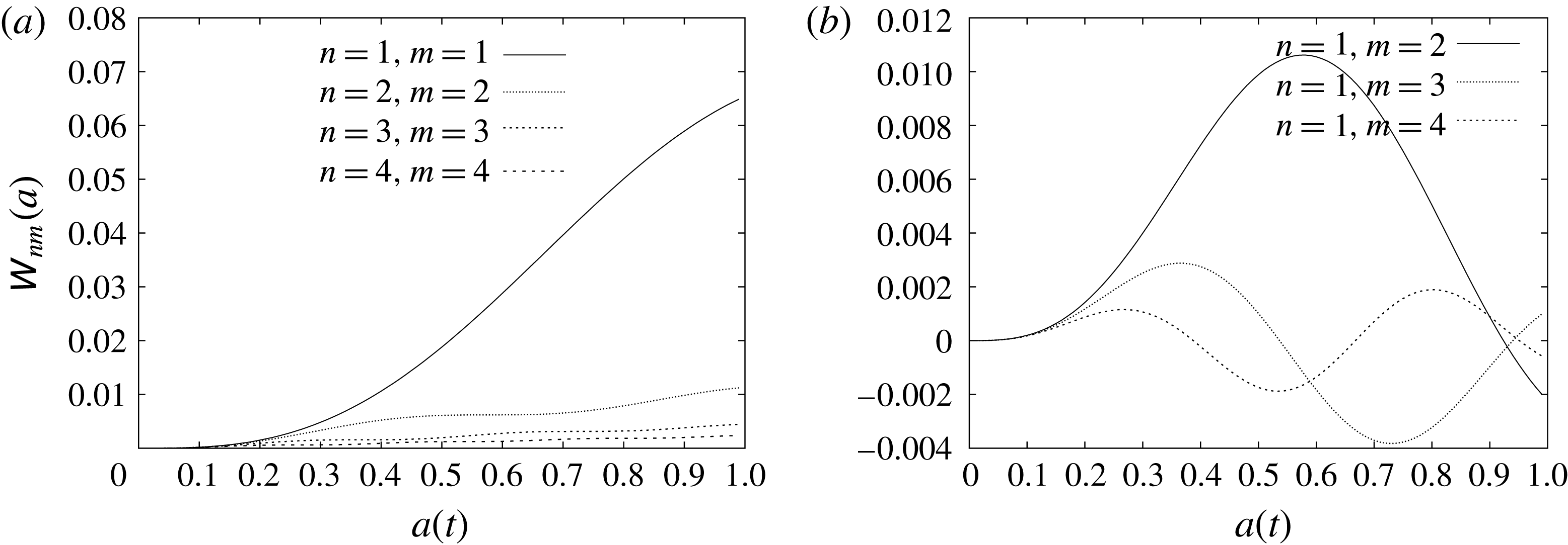
It was confirmed numerically that the solution converges with increasing number of modes and that the number of modes used in our calculations captures the physics of the full system with sufficient accuracy. We confirmed the convergence with number of modes by analysing in particular the behaviour of the added-mass matrix,
 $\unicode[STIX]{x1D652}(a)$
. It was found that as the number of modes increases the elements of the added-mass matrix rapidly decay, as will be seen in appendix D, figure 21. The convergence with number of modes was found to be fairly good – with ten modes providing very good accuracy during the impact stage with a partially wetted plate. Later, when the elastic plate is fully wetted, the method is found to have substantially better convergence – with five modes providing an adequate long-term representation of the flow and plate deflection. This stems from the elastic effects (and hence the added-mass contribution) becoming much less important compared with the rigid terms during the stage with a fully wetted plate.
Once (5.1)–(5.4) have been resolved the jet thickness (4.6) yields conditions providing the time splashing is observed. For negative acceleration
 $\ddot{a}(\unicode[STIX]{x1D70F})$
, we have
 $$\begin{eqnarray}1-\frac{2\ddot{a}(\unicode[STIX]{x1D70F})(t-\unicode[STIX]{x1D70F})}{{\dot{a}}(\unicode[STIX]{x1D70F})}=1+\frac{2|\ddot{a}(\unicode[STIX]{x1D70F})|(t-\unicode[STIX]{x1D70F})}{{\dot{a}}(\unicode[STIX]{x1D70F})}\geqslant 1,\end{eqnarray}$$
where
 $t\geqslant \unicode[STIX]{x1D70F}$
. If
 $\ddot{a}(\unicode[STIX]{x1D70F})>0$
for a certain
 $\unicode[STIX]{x1D70F}$
, then
 $h(r,t)\rightarrow \infty$
as
 $t\rightarrow t_{c}(\unicode[STIX]{x1D70F})$
, where
 $t_{c}(\unicode[STIX]{x1D70F})$
is determined by the equation
 $$\begin{eqnarray}\frac{2\ddot{a}(\unicode[STIX]{x1D70F})}{{\dot{a}}(\unicode[STIX]{x1D70F})}(t_{c}(\unicode[STIX]{x1D70F})-\unicode[STIX]{x1D70F})=1,\end{eqnarray}$$
and
 $t_{c}(\unicode[STIX]{x1D70F})>\unicode[STIX]{x1D70F}$
. For a given function
 $a(\unicode[STIX]{x1D70F})$
, to determine the position and time of formation of the splash we need to find the minimum value,
 $t_{min}$
, of the function
 $t_{c}(\unicode[STIX]{x1D70F})$
. To calculate
 $t_{min}$
and the radius
 $r_{s}$
at which the splashing occurs, we find the maxima of
 $$\begin{eqnarray}\frac{1}{t_{c}(\unicode[STIX]{x1D70F})}=\frac{2\ddot{a}(\unicode[STIX]{x1D70F})}{{\dot{a}}(\unicode[STIX]{x1D70F})+2\unicode[STIX]{x1D70F}\ddot{a}(\unicode[STIX]{x1D70F})},\end{eqnarray}$$
with the constraint that
 $$\begin{eqnarray}0<\frac{1}{t_{c}(\unicode[STIX]{x1D70F})}<\frac{1}{\unicode[STIX]{x1D70F}}.\end{eqnarray}$$
This approach provides a graphical way to find the time
 $t_{min}$
and the corresponding value of
 $\unicode[STIX]{x1D70F}=\unicode[STIX]{x1D70F}_{min}$
, such that
 $t_{c}(\unicode[STIX]{x1D70F}_{min})=t_{min}$
. The radius
 $r_{s}$
at which splashing occurs then follows from (4.5):
 $$\begin{eqnarray}r_{s}=a(\unicode[STIX]{x1D70F}_{min})+\frac{{\dot{a}}^{2}(\unicode[STIX]{x1D70F}_{min})}{\ddot{a}(\unicode[STIX]{x1D70F}_{min})}.\end{eqnarray}$$
Although the elastic plate motion additionally affects fine details of the jet behaviour through the initial jet thickness
 $H_{j}$
(see (3.39) and (4.1)), its primary effect is to be responsible for triggering blow-up of the jet through the varying acceleration of the contact line.
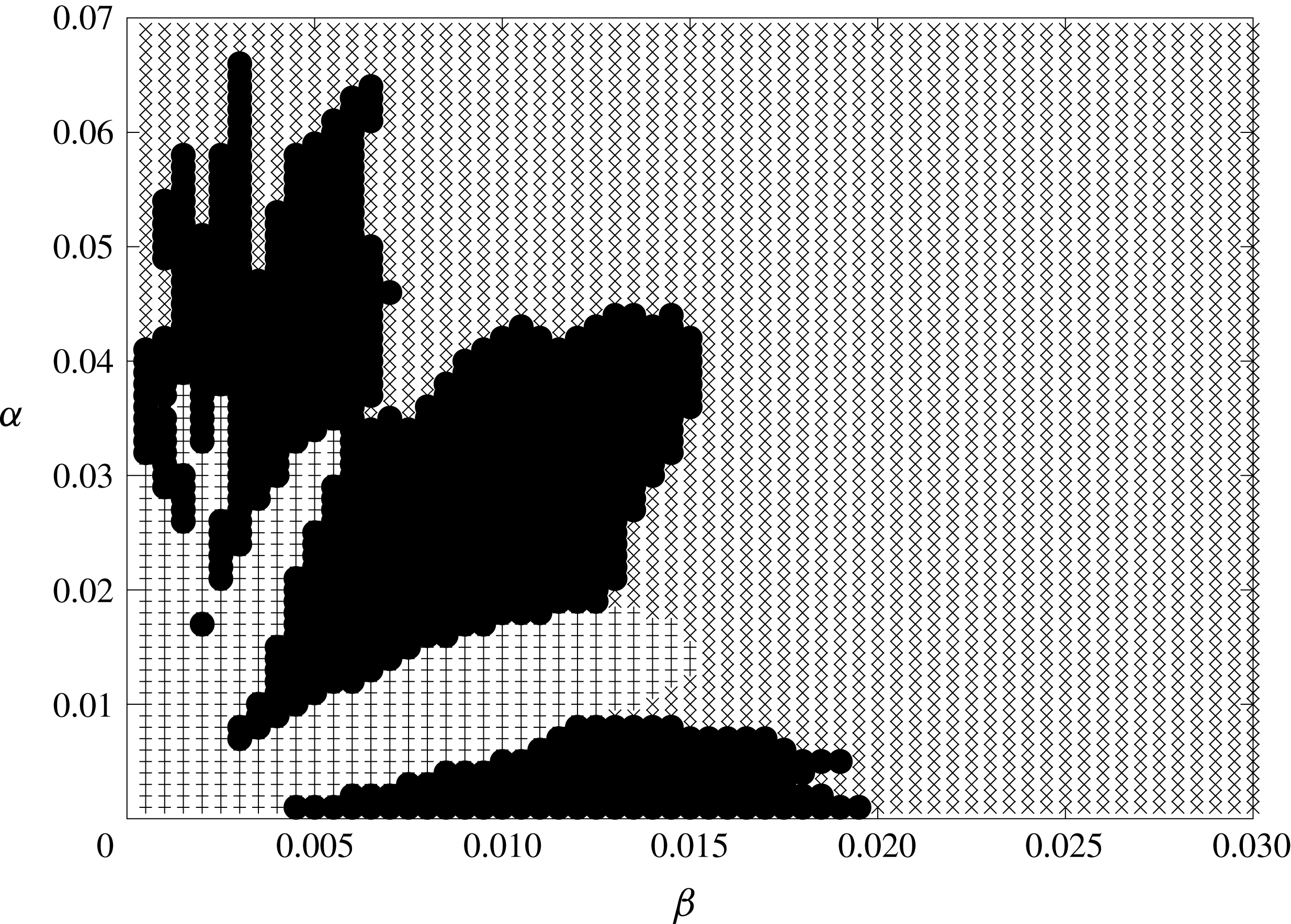
Parametric plane showing the regions of negative and unbounded contact line velocity. Pluses represent simulations which encounter contact line shrinkage, crosses represent simulations with no problems, and filled circles represent simulations with an unbounded contact line velocity.

Although the method of normal modes provides a good basis to investigate the velocity field in the droplet, plate deflection and elastic stresses, it does not allow us to accurately determine the pressure distribution over the wetted region. The pressure singularity at the contact line, coupled with poor convergence of the modal series for the plate acceleration
 $w_{tt}(r,t)$
, make a series representation of the pressure impractical, as discussed by Korobkin (Reference Korobkin1998). However, our main goal in this paper is to study the effect of elasticity on the spreading and splashing of a droplet. We assume that the pressure in the wetted part of the substrate does not go down to the vapour pressure due to the elastic plate vibration. If so, cavitation does not occur, and both the spreading and splashing of the droplet are not affected by the details of the pressure distribution.
6 Results
The problem described above is entirely governed by two non-dimensional parameters
 $\unicode[STIX]{x1D6FC}$
and
 $\unicode[STIX]{x1D6FD}$
, as defined in (2.9). Solutions have been calculated across the entirety of the
 $\unicode[STIX]{x1D6FC}$
–
 $\unicode[STIX]{x1D6FD}$
parameter space by solving (5.2)–(5.4), along with subsequently determining the characteristics of the splash jets. Before discussing these results in more detail, we note that there are values of
 $\unicode[STIX]{x1D6FC}$
and
 $\unicode[STIX]{x1D6FD}$
for which solutions cannot be found. Due to constraints of the Wagner approach adopted here, our model breaks down if the contact region begins to shrink,
 $\text{d}a/\text{d}t<0$
, or if the velocity of the contact region expansion becomes comparable to the speed of sound in the liquid for
 $t>0$
. This means that for some values of the parameters
 $\unicode[STIX]{x1D6FC}$
and
 $\unicode[STIX]{x1D6FD}$
in (2.8) the simulations cannot be completed up to the time the plate is fully wetted. Figure 3 depicts the regions in the parametric plane
 $(\unicode[STIX]{x1D6FC},\unicode[STIX]{x1D6FD})$
where these two types of failure were found. It is seen that the regions of failure are limited to small values of both
 $\unicode[STIX]{x1D6FC}$
and
 $\unicode[STIX]{x1D6FD}$
. Wagner theory can be used for any values of
 $\unicode[STIX]{x1D6FD}$
if
 $\unicode[STIX]{x1D6FC}>0.07$
. For an aluminium plate, with density
 $\unicode[STIX]{x1D70C}_{p}=2700~\text{kg}~\text{m}^{-3}$
, radius
 $L=1~\text{mm}$
and a water droplet of density
 $\unicode[STIX]{x1D70C}=1000~\text{kg}~\text{m}^{-3}$
, this inequality requires the thickness of the plate to be greater than
 $26~\unicode[STIX]{x03BC}\text{m}$
. The magnitudes of
 $\unicode[STIX]{x1D6FC}$
and
 $\unicode[STIX]{x1D6FD}$
in these excluded regions match those found by Korobkin & Khabakhpasheva (Reference Korobkin and Khabakhpasheva2006) in the related two-dimensional problem of water wave impact onto an elastic plate, although the details are different. Both types of failure are observed to occur at a relatively late stage of the impact, when the main part of the elastic plate has been wetted.
To understand the physical reasons for the very small and very large predicted velocities of the contact line when the validity of our model breaks down, note that the denominator in (5.1) corresponds to the relative velocity of impact, and the numerator corresponds to the relative angle between the undisturbed far-field droplet shape and the shape of the deformed elastic plate. This becomes more transparent if we return to the Wagner condition (2.21) for the radius of the contact region
 $a(t)$
, differentiate it in time, and introduce the new variable of integration,
 $r=a(t)\sin (\unicode[STIX]{x1D703})$
,
 $$\begin{eqnarray}\frac{\text{d}a}{\text{d}t}\frac{1}{a^{2}}\int _{0}^{a}\left(r+\frac{\unicode[STIX]{x2202}w}{\unicode[STIX]{x2202}r}(r,t)\right)\frac{r^{2}\,\text{d}r}{\sqrt{a^{2}-r^{2}}}=\frac{1}{a}\int _{0}^{a}\left(1-\frac{\unicode[STIX]{x2202}w}{\unicode[STIX]{x2202}t}(r,t)\right)\frac{r\,\text{d}r}{\sqrt{a^{2}-r^{2}}}.\end{eqnarray}$$
In (6.1),
 $r$
in the first integral corresponds to the slope of the initial shape of the droplet and
 $\unicode[STIX]{x2202}w/\unicode[STIX]{x2202}r$
corresponds to the slope of the deformed plate in the contact region,
 $0<r<a$
. The integral on the left-hand side of (6.1) divided by
 $a^{2}$
represents the averaged difference of the slopes with the weighting
 $r^{2}/\sqrt{a^{2}-r^{2}}$
. The weighting determines the relative importance of the local difference in slope and indicates that the value of the integral depends mainly on the relative slope near the contact line. Similar arguments hold for the integral on the right-hand side of (6.1). This integral divided by
 $a$
is the averaged relative velocity of the impact with weighting
 $r/\sqrt{a^{2}-r^{2}}$
. Both integrals should remain positive within the assumptions underlying the Wagner condition. If the velocity of the plate deflection,
 $\unicode[STIX]{x2202}w/\unicode[STIX]{x2202}t$
, becomes too large and the integral in the right-hand side of (6.1) approaches zero, then
 $\text{d}a/\text{d}t$
also approaches zero and the contact region stops expanding. This type of failure is shown in figure 3 by pluses. This failure mode is illustrated by figures 4 and 5 for
 $\unicode[STIX]{x1D6FC}=0.01$
and
 $\unicode[STIX]{x1D6FD}=0.001$
. These values of the non-dimensional parameters
 $\unicode[STIX]{x1D6FC}$
and
 $\unicode[STIX]{x1D6FD}$
imply that for the aluminium plate of radius 1 mm and droplet radius 5 mm, the impact speed is
 $9.67~\text{m}~\text{s}^{-1}$
and the elastic plate thickness is
 $3.7~\unicode[STIX]{x03BC}\text{m}$
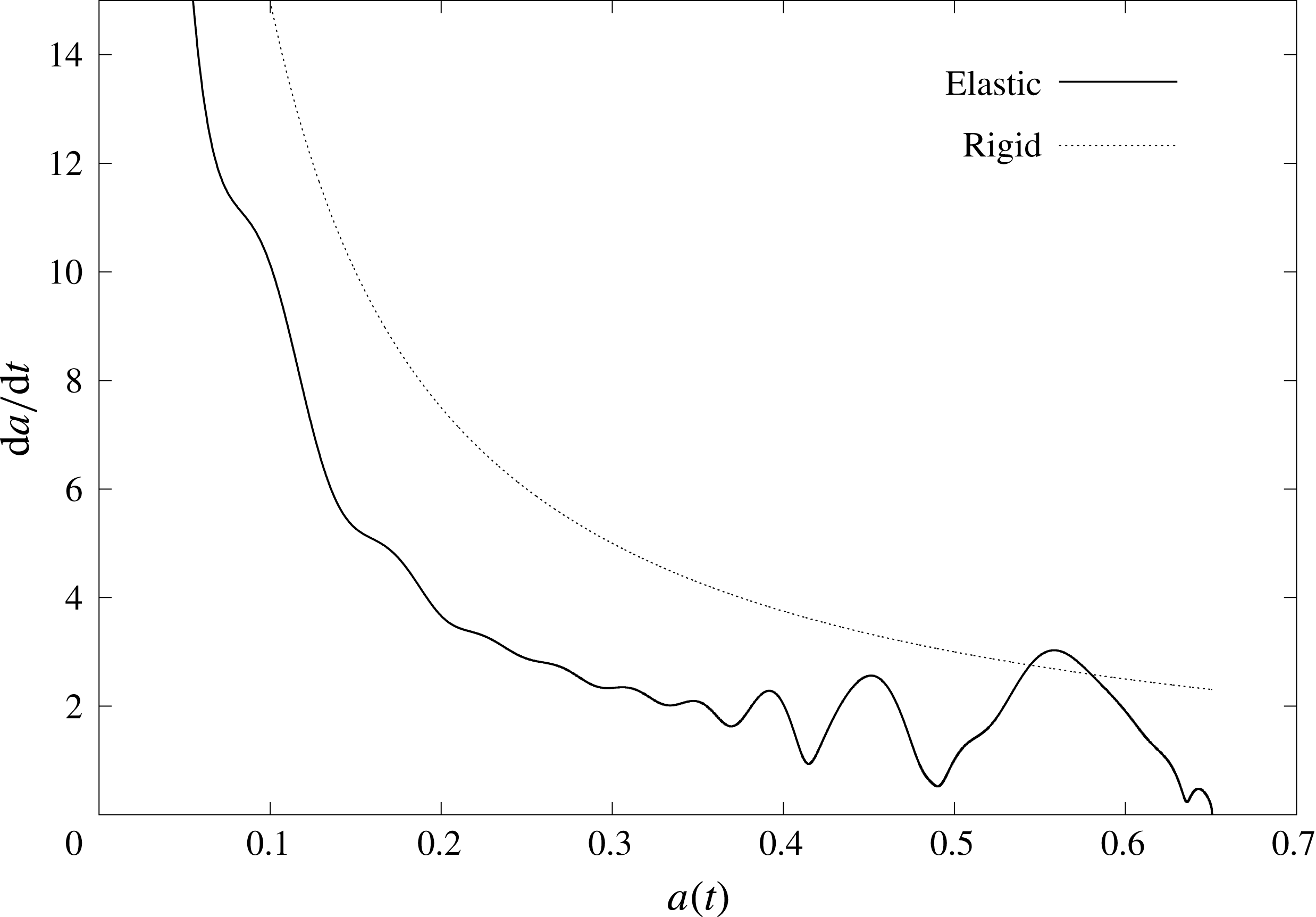
. Figure 4 shows that the non-dimensional contact line speed,
 $\text{d}a/\text{d}t$
, for this elastic plate is smaller than that for the corresponding rigid substrate, and the contact line speed starts oscillating at
 $a\approx 0.65$
, well before the plate is fully wetted. The averaged plate deflection and velocity,
 $$\begin{eqnarray}\int _{0}^{1}w(r,t)r\,\text{d}r,\quad \int _{0}^{1}w_{t}(r,t)r\,\text{d}r,\end{eqnarray}$$
are shown in figure 5. Both the averaged deflection and velocity are very small for
 $0<a\leqslant 0.2$
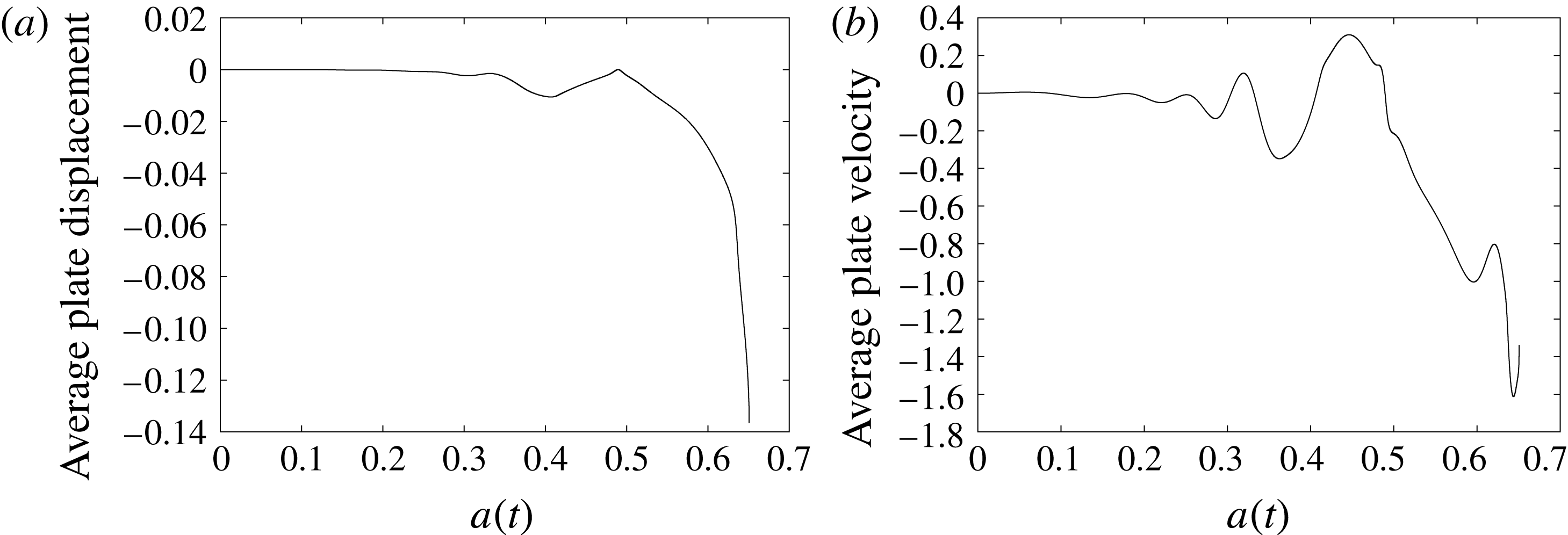
. However, the plate deflection cannot be neglected even during this initial phase. The effect of the plate deflection on the speed of the contact line is significant (see figure 4). Note that the acceleration of the contact line,
 $\text{d}^{2}a/\text{d}t^{2}$
, is always negative for rigid plates, but oscillates for the elastic plate.
The second distinct failure occurs where the slope of the deformed plate,
 $-\unicode[STIX]{x2202}w/\unicode[STIX]{x2202}r$
, becomes large and approaches the slope,
 $r$
, of the free surface of the undisturbed droplet. In this regime, the integral on the left-hand side of (6.1) approaches zero and
 $\text{d}a/\text{d}t\rightarrow \infty$
. This second type of failure is related to the shape of the deformed plate. When the shapes of the elastic plate and impacting free surface have the same gradient near the contact line, Wagner theory predicts that the plate can be instantly wetted. Physically this corresponds to touchdown occurring simultaneously over a finite region of the plate rather than via a moving contact line. This causes the unrealistically extremely large contact line velocity found in the results, and the failure of our model.
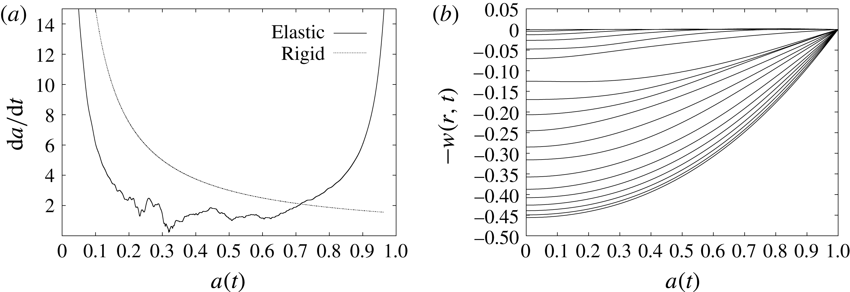
The non-dimensional speed of the contact line and the shapes of the plate at time instants corresponding to the radius of the contact line with a step of
 $0.05$
from
 $a=0$
to
 $a=0.9$
are shown in figure 6 for
 $\unicode[STIX]{x1D6FC}=0.005$
and
 $\unicode[STIX]{x1D6FD}=0.014$
. These values of
 $\unicode[STIX]{x1D6FC}$
and
 $\unicode[STIX]{x1D6FD}$
correspond to an aluminium plate of radius 1 mm and the thickness
 $2~\unicode[STIX]{x03BC}\text{m}$
impacted by a droplet of water with radius 5 mm and speed
 $0.9~\text{m}~\text{s}^{-1}$
. The speed of the contact line becomes unbounded shortly before the plate is completely wetted. When the elastic plate is partially wetted the contact region expands more slowly than for a rigid plate, which qualitatively agrees with the results by Pepper et al. (Reference Pepper, Courbin and Stone2008). This is not typically true as the contact line approaches the edge of the plate. This phenomenon was not observed by Pepper et al. (Reference Pepper, Courbin and Stone2008), where an elastic film of large radius was considered. The early stages, where the wetted region is far smaller than the elastic plate, act as an approximation to the situation investigated by Pepper et al. (Reference Pepper, Courbin and Stone2008).
Contact line velocity
 $\text{d}a/\text{d}t$
for
 $\unicode[STIX]{x1D6FC}=0.01$
,
 $\unicode[STIX]{x1D6FD}=0.001$
as a function of the non-dimensional contact line radius
 $a(t)$
.

The averaged plate displacement (a) and averaged plate velocity (b) for
 $\unicode[STIX]{x1D6FC}=0.01$
,
 $\unicode[STIX]{x1D6FD}=0.001$
as functions of the contact line radius
 $a$
.

The contact line velocity (a) and plate shapes (b) calculated at intervals of
 $a=0.05$
for
 $\unicode[STIX]{x1D6FC}=0.005$
,
 $\unicode[STIX]{x1D6FD}=0.014$
.

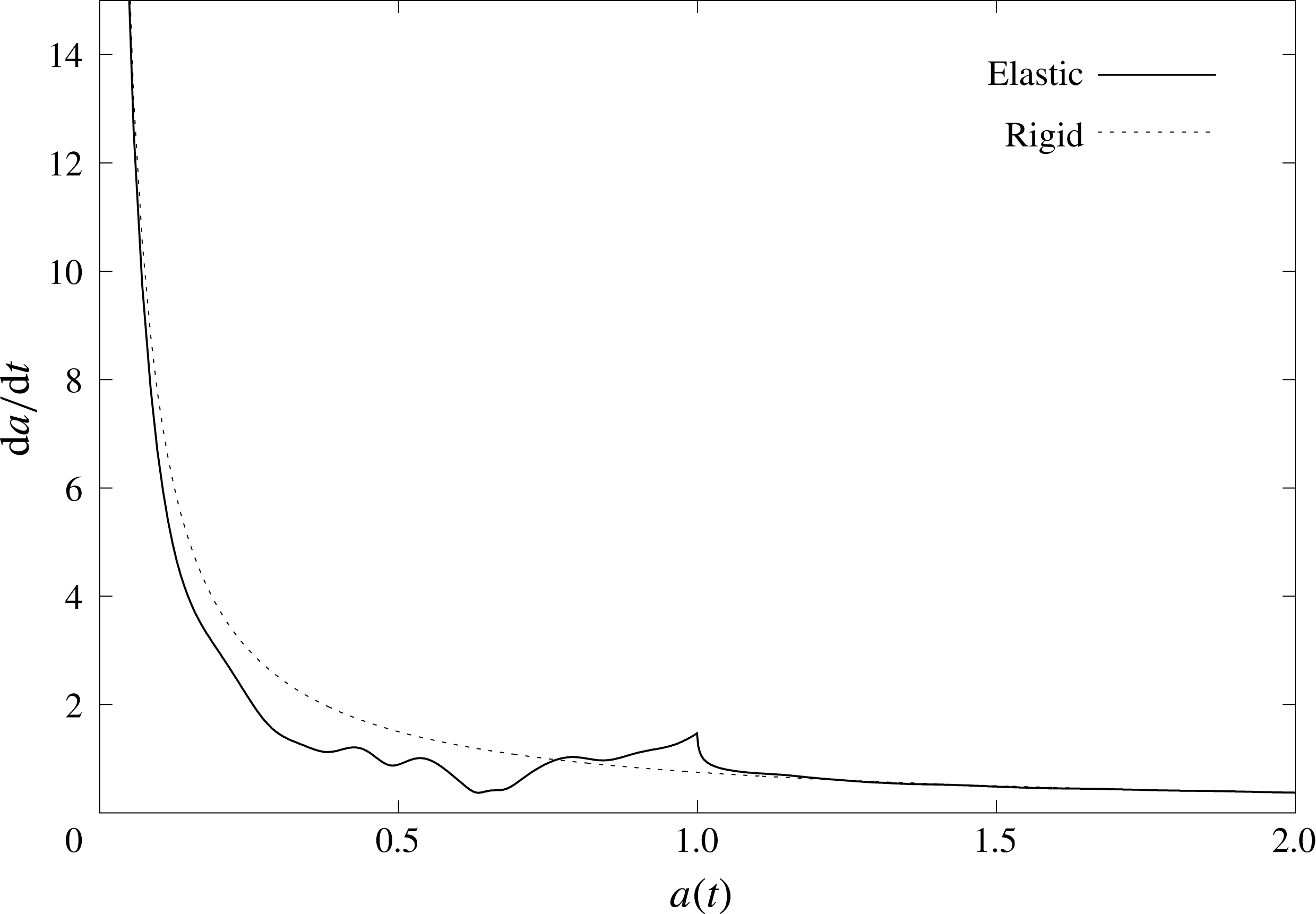
Since the slope of the substrate is discontinuous at the edge of the simply supported elastic plate, the contact line speed is also discontinuous there. This discontinuity is well described by the Wagner theory, as shown in figure 7 for an aluminium plate with parameters
 $\unicode[STIX]{x1D6FC}=0.1$
and
 $\unicode[STIX]{x1D6FD}=0.01$
. This figure demonstrates that, as the contact line advances beyond the edge of the elastic plate, the influence of the plate vibrations on the contact line velocity decays rapidly. Calculations were also performed with different end conditions for the elastic plate, in particular with clamped ends rather than simply supported; whilst the quantitative details of contact line velocity and plate behaviour are markedly different, the same splashing mechanism described below is still observed. This suggests that the edge discontinuity does not affect the underlying trigger for splashing.
Contact line velocity
 $\text{d}a/\text{d}t$
for
 $\unicode[STIX]{x1D6FC}=0.1$
,
 $\unicode[STIX]{x1D6FD}=0.01$
as a function of contact line radius
 $a$
.

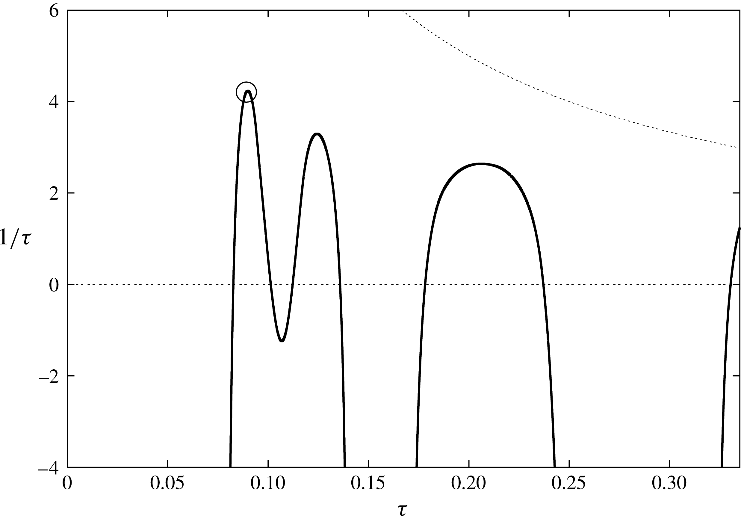
Figure 8 illustrates the method to determine the conditions of splashing; see § 5. Splashing occurs for any
 $\unicode[STIX]{x1D70F}$
such that the function
 $1/t_{c}(\unicode[STIX]{x1D70F})$
, given by (5.9) and shown in figure 8 by the solid line, satisfies both inequalities in (5.10). The limits in (5.10) are shown by dotted lines in figure 8. The earliest time of splashing,
 $t_{min}$
, corresponds to the maximum of
 $1/t_{c}(\unicode[STIX]{x1D70F})$
under conditions (5.10). This value is shown in figure 8 by a circle marker. Splashing occurs also for liquid particles with their Lagrangian coordinates
 $\unicode[STIX]{x1D70F}$
approximately 0.2 and 0.35 but slightly later than for the earliest splash and in different locations. For the parameters shown in figure 8 we can see that the first splash occurs at
 $\unicode[STIX]{x1D70F}=0.071$
and is seen at approximate non-dimensional time
 $t=1/3.87\approx 0.258$
. It is expected that surface tension and viscosity may smooth the predicted splash. Profiles of the jet thickness as functions of the radial coordinate
 $r>a(t)$
, at
 $t=0.07,0.12$
and
 $0.19$
are shown in figure 9(a) and in figure 9(b) as functions of the Lagrangian coordinate
 $\unicode[STIX]{x1D70F}$
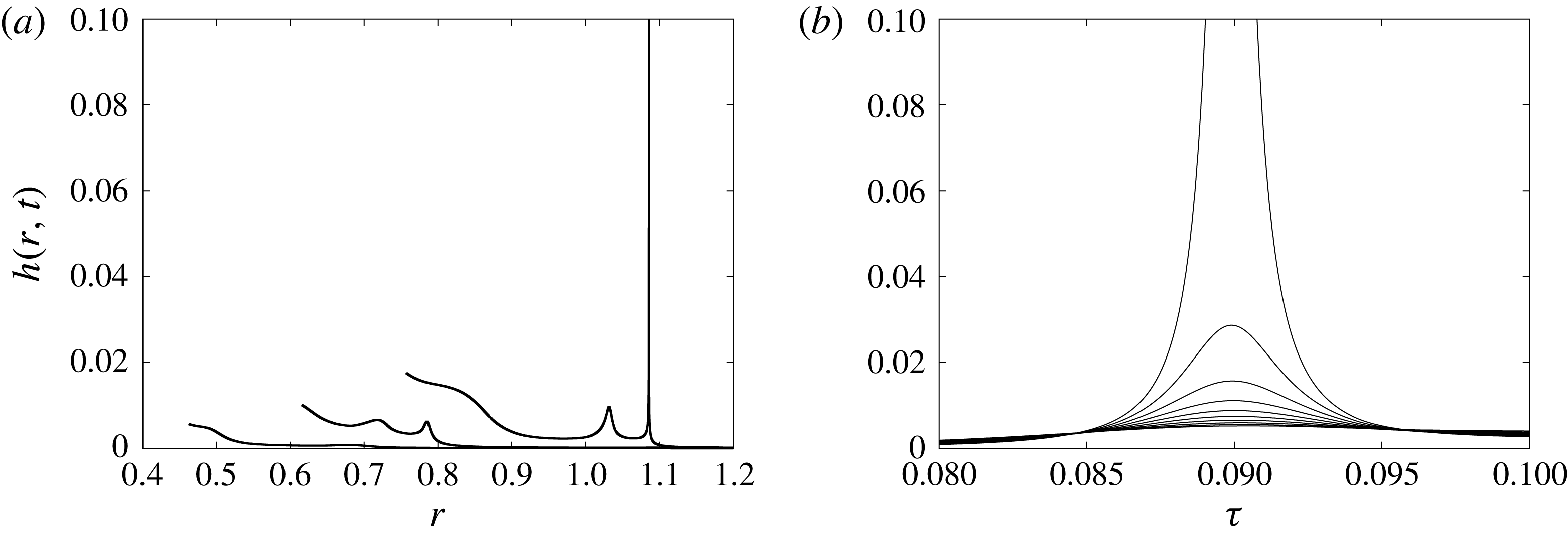
at different time instants. It is seen that the jet thickness decreases in front of and behind the liquid particle at which splashing occurs.


For the parameters
 $\unicode[STIX]{x1D6FC}=0.1$
and
 $\unicode[STIX]{x1D6FD}=0.3$
, (a) shows the jet thickness
 $h(r,t)$
given by (4.6) as the function of
 $r$
, where
 $r>a(t)$
for
 $t=0.07$
, 0.12 and 0.19 and (b) shows the growth of the splash for the interval
 $0.08<\unicode[STIX]{x1D70F}<0.105$
of the Lagrangian coordinate
 $\unicode[STIX]{x1D70F}$
, from time
 $t=0.145$
to
 $t=0.235$
in steps of
 $0.01$
. Increasing time is shown by an increasing maximum in both plots.

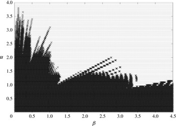
The region of the parametric plane (
 $\unicode[STIX]{x1D6FC},\unicode[STIX]{x1D6FD}$
) where splashing can occur is large (see figure 10), and includes all cases studied above. As parameter pairs come closer to the edge of the splashing region, the time in which we see the splash occur grows rapidly.
The
 $\unicode[STIX]{x1D6FC}-\unicode[STIX]{x1D6FD}$
parametric plot where splashing is predicted (dark crossed region) and where it is not predicted (dotted region).

To give further insight into the predicted behaviour of our model, figures 11–18 show variations in contact line velocity, plate deformation and jet profiles for a selection of parameters. Considering a 1 cm radius water droplet impacting a 1 mm radius aluminium plate at a speed of
 $2.5~\text{ms}^{-1}$
, we present results for three plate thicknesses 0.1, 0.065 and 0.04 mm. These choices correspond to our non-dimensional numbers being given by
 $\unicode[STIX]{x1D6FC}=0.27,0.175,0.108$
and
 $\unicode[STIX]{x1D6FD}=10.6,2.91,0.678$
, respectively. Physically they represent three distinct cases: no splashing predicted (0.1 mm), on the borderline of splashing (0.065 mm) and splashing (0.04 mm). This can be seen in figure 10.
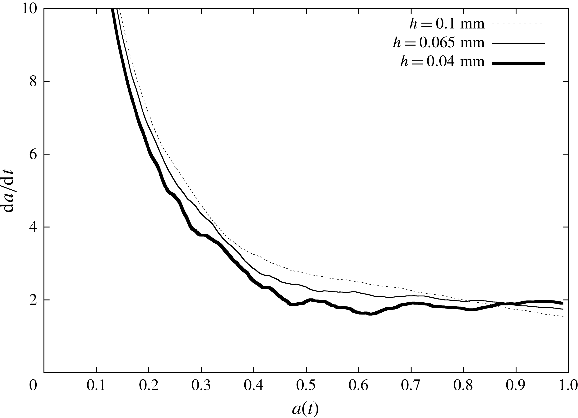
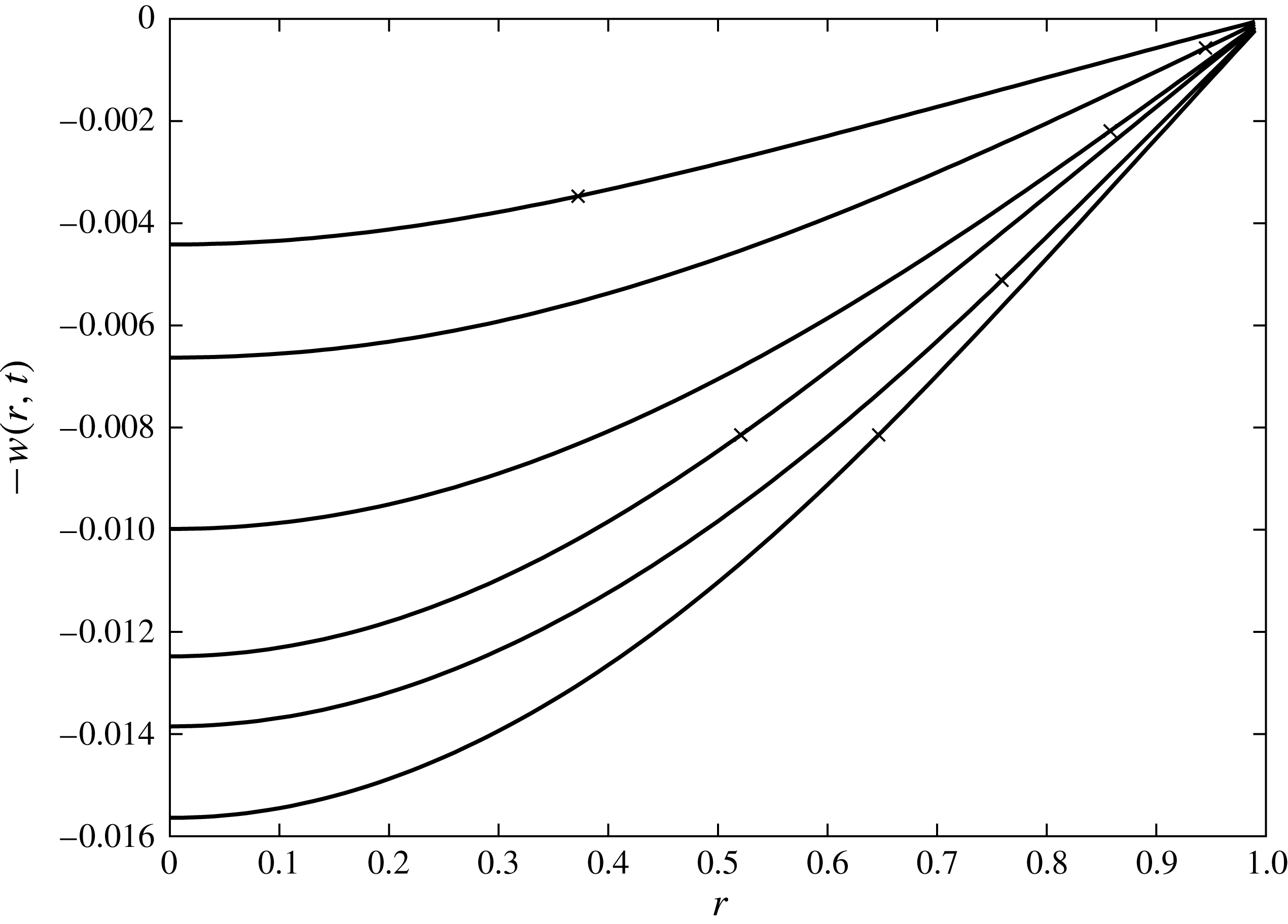
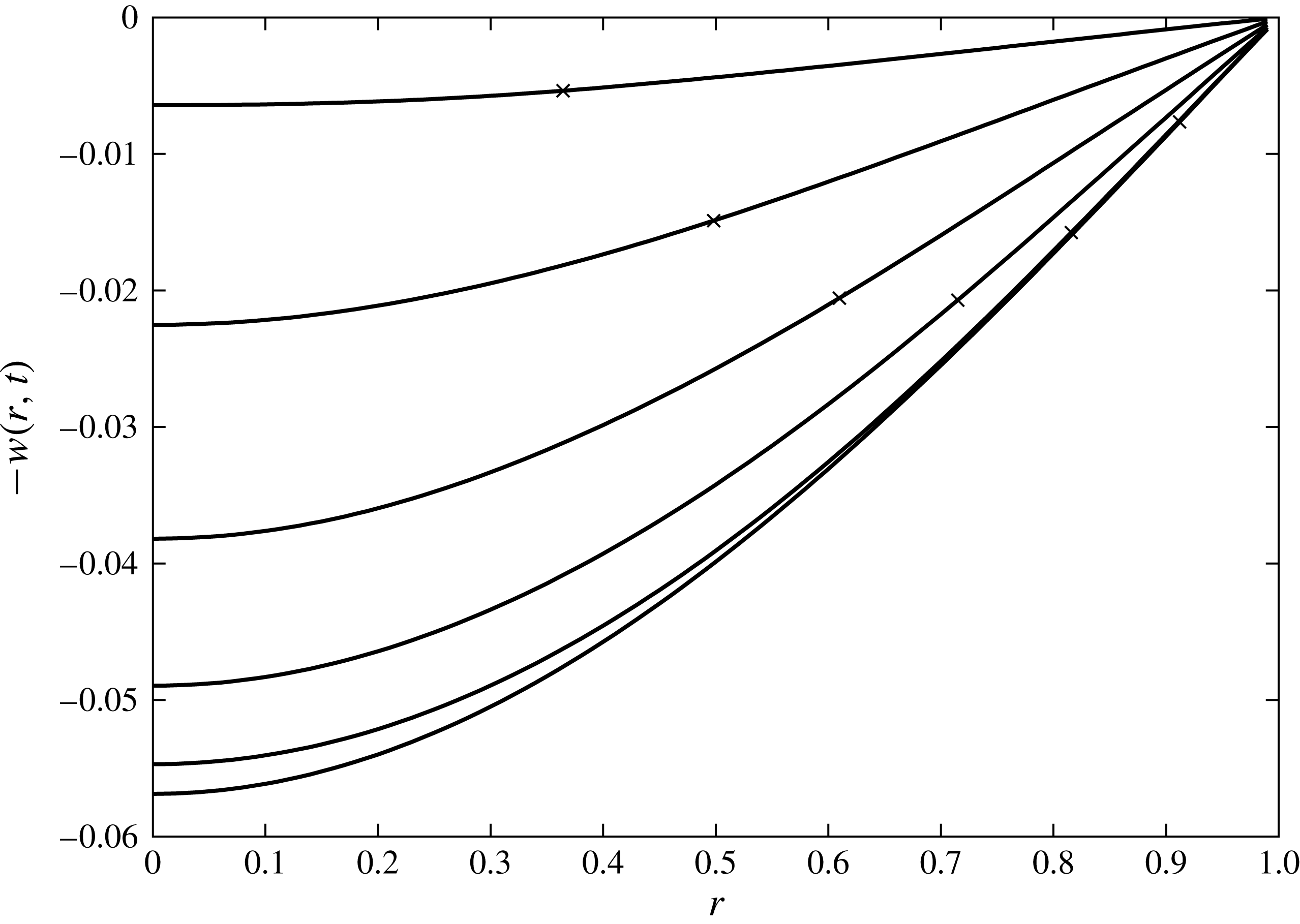
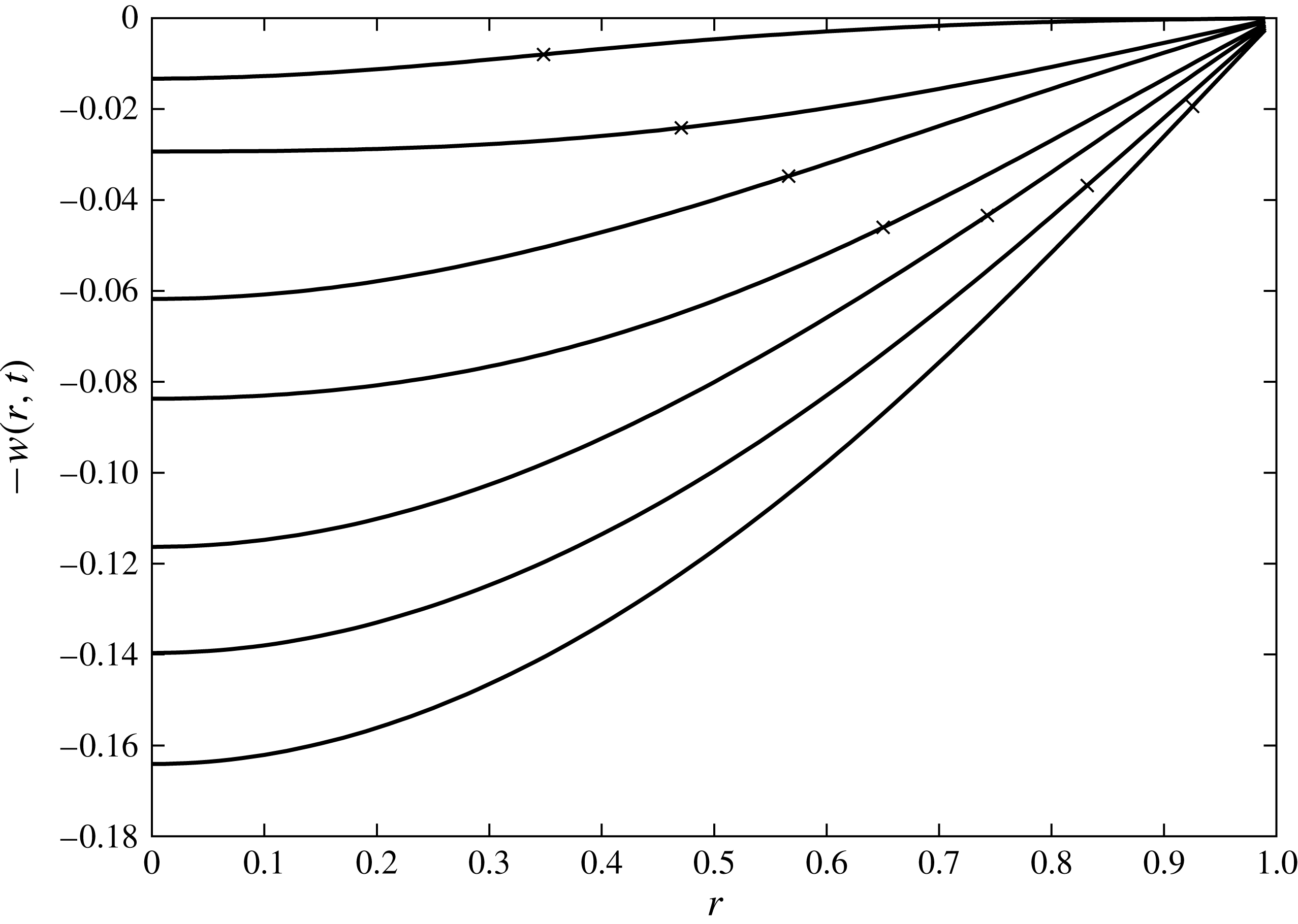
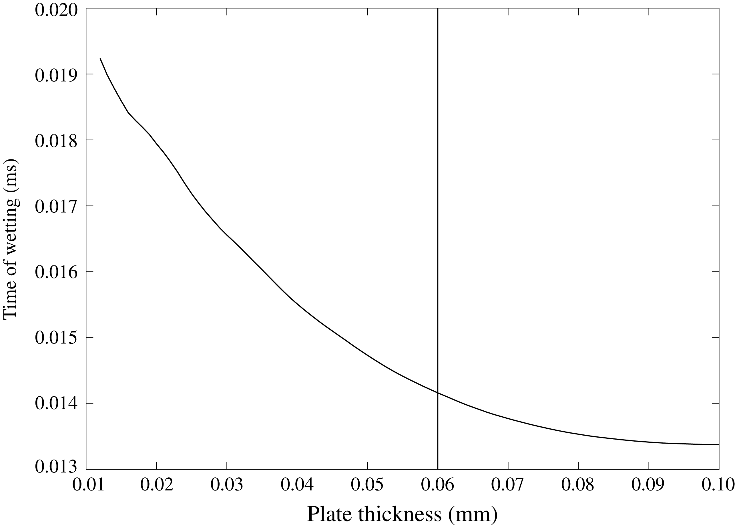
Considering the contact line velocity in figure 11, the thickest plate (which does not splash) follows very closely the behaviour of a rigid plate. Note that, although the borderline case does demonstrate some oscillatory behaviour, the acceleration of the contact line never becomes positive, in contrast to the 0.04 mm case, which does exhibit splashing. The shapes of the elastic plates are shown in figures 12 (0.1 mm), 13 (0.065 mm) and 14 (0.04 mm) at fixed times. The more elastic substrates deform substantially further and faster. The large displacements can result in a much longer time until the plate is completely wetted, as plotted in figure 15.
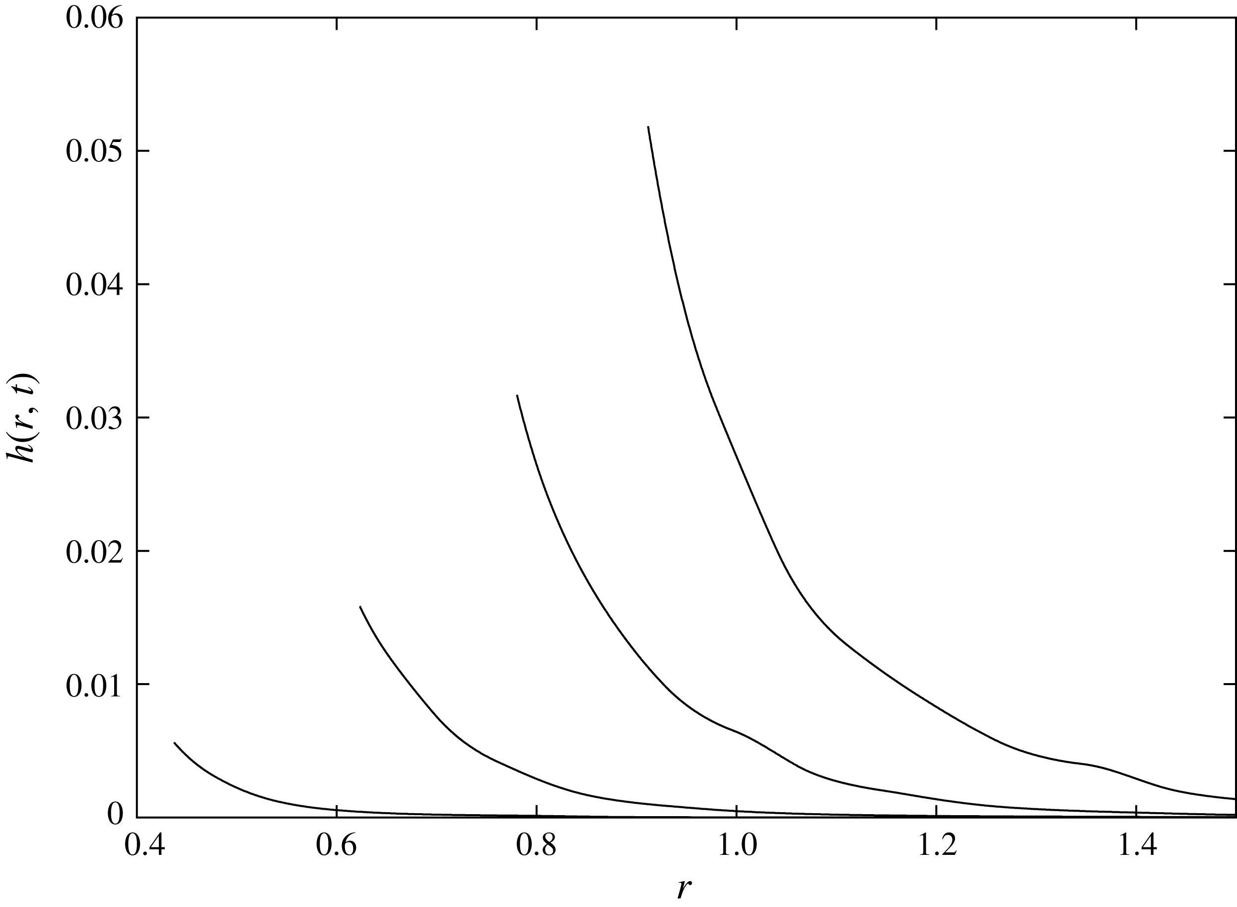
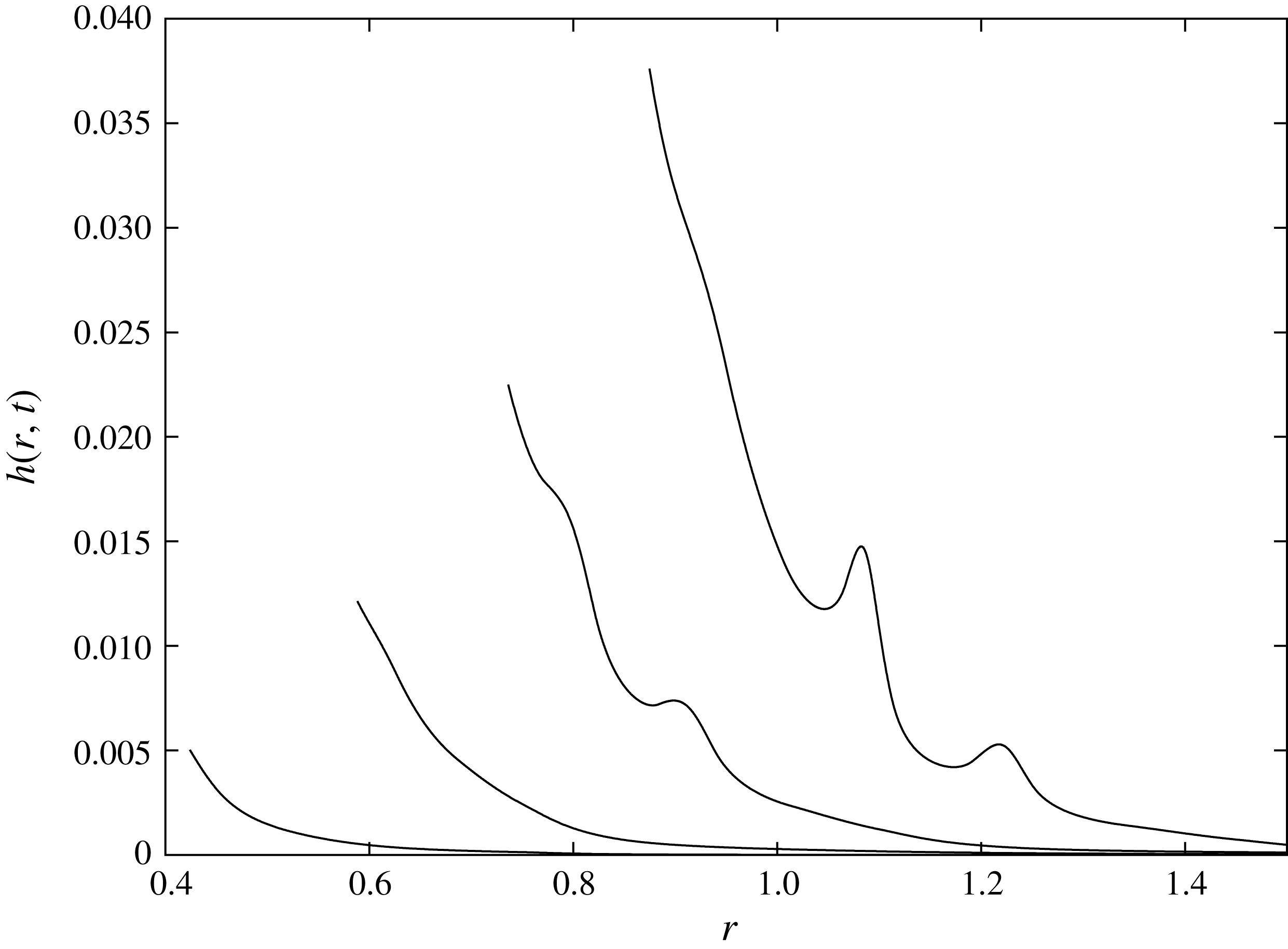
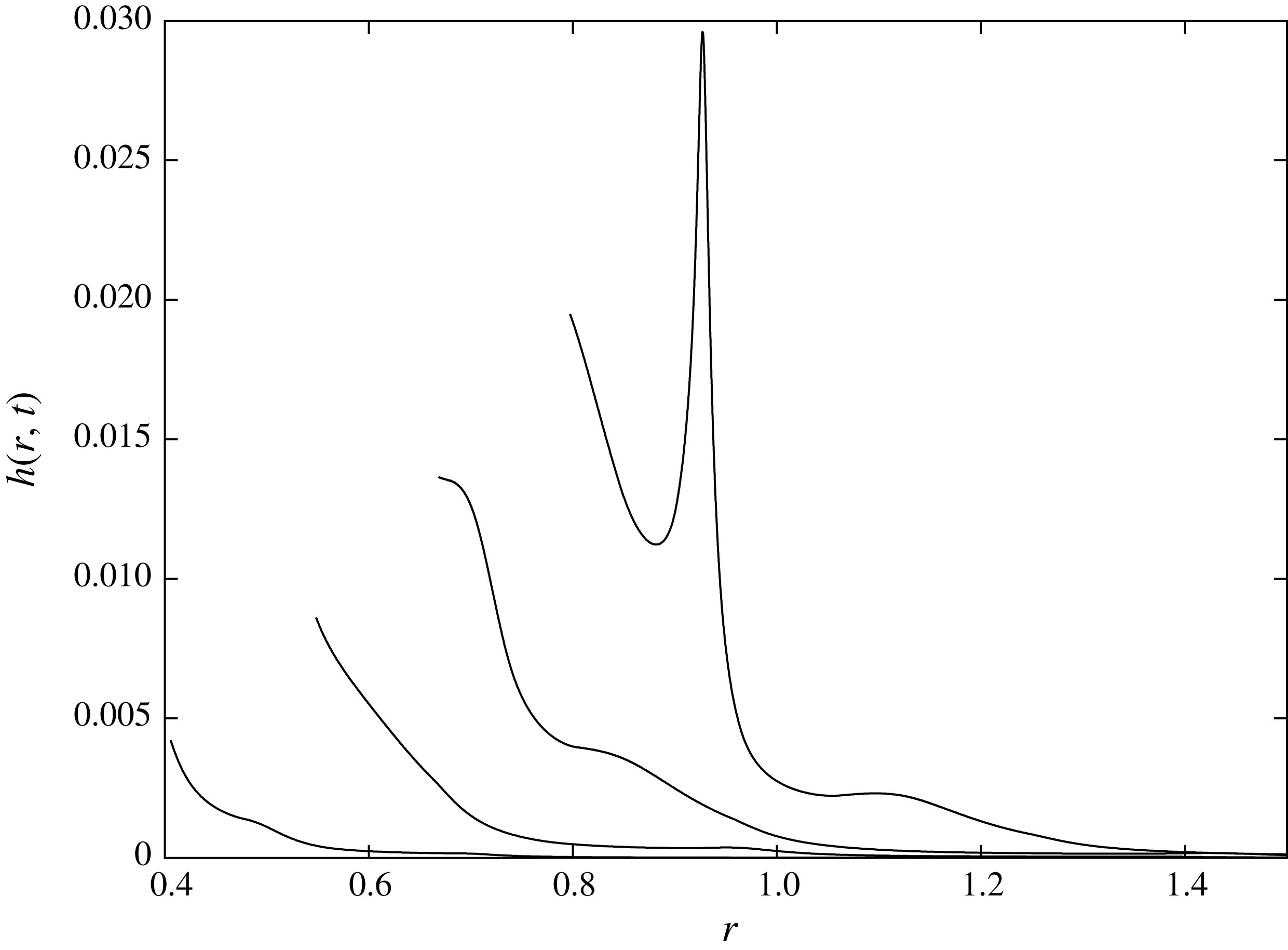
Profiles of the evolving splash jet are plotted in figures 16 (0.1 mm), 17 (0.065 mm) and 18 (0.04 mm). Oscillations of the elastic plate, and subsequent effects on the contact line velocity, can be seen to cause disturbances in the jet profiles even in the non-splashing cases. Due to the contact line acceleration never becoming positive, these disturbances can be observed not to grow in figures 16 and 17, whilst in figure 18 the initial disturbance grows and leads to blow-up in the thin jet, and subsequent splashing.
Contact line velocity for
 $\unicode[STIX]{x1D6FC}=0.27,\unicode[STIX]{x1D6FD}=10.6$
.
 $\unicode[STIX]{x1D6FC}=0.175,\unicode[STIX]{x1D6FD}=2.911$
and
 $\unicode[STIX]{x1D6FC}=0.108,\unicode[STIX]{x1D6FD}=0.678$
.

Plate displacement calculated at times
 $t=0.05,0.1,0.15,0.2,0.25,0.3$
for
 $\unicode[STIX]{x1D6FC}=0.27$
and
 $\unicode[STIX]{x1D6FD}=10.6$
(
 $h=0.1$
mm). Crosses indicate the position of the contact line.

Plate displacement calculated at times
 $t=0.05,0.1,0.15,0.2,0.25,0.3$
for
 $\unicode[STIX]{x1D6FC}=0.175$
and
 $\unicode[STIX]{x1D6FD}=2.911$
(
 $h=0.065~\text{mm}$
). Crosses indicate the position of the contact line.

Plate displacement calculated at times
 $t=0.05,0.1,0.15,0.2,0.25,0.3$
for
 $\unicode[STIX]{x1D6FC}=0.108$
and
 $\unicode[STIX]{x1D6FD}=0.678$
(
 $h=0.04~\text{mm}$
). Crosses indicate the position of the contact line.

Dimensional time at which the plate is fully wetted versus plate thickness for a 1 cm water droplet impacting a 1 mm radius aluminium plate at
 $2.5~\text{ms}^{-1}$
. The vertical line separates the splashing regimes to the left and non-splashing to the right.

Jet profile for
 $\unicode[STIX]{x1D6FC}=0.27,\unicode[STIX]{x1D6FD}=10.6$
(
 $h=0.1~\text{mm}$
) at times
 $t=0.07,0.14,0.21,0.28$
.

Jet profile for
 $\unicode[STIX]{x1D6FC}=0.175,\unicode[STIX]{x1D6FD}=2.91$
(
 $h=0.065~\text{mm}$
) at times
 $t=0.07,0.14,0.21,0.28$
.

Jet profile for
 $\unicode[STIX]{x1D6FC}=0.108,\unicode[STIX]{x1D6FD}=0.678$
(
 $h=0.04~\text{mm}$
) at times
 $t=0.07,0.14,0.21,0.28$
.

7 Conclusion
A model of droplet impact onto an elastic plate has been presented. The model generalises the Wagner theory of water impact to axisymmetric configurations and an elastic surface of the body. The uniformly valid description of the resulting flow was obtained using the asymptotic approach by Howison et al. (Reference Howison, Ockendon and Wilson1991). The flow region is divided into three subregions: the main flow region with its size on order of the elastic plate diameter; the small jet-root region at the periphery of the wetted part of the substrate; and the jet region where splashing can be observed. The pressure and velocity field of the main flow region are singular at the contact line, necessitating the formation of an asymptotic jet root close to the contact line. In order to conserve mass, a liquid jet emanates from the jet-root region in a direction normal to the contact line. It was shown that the vibrating substrate does not directly interact with the jet-root region at leading order, only providing a contribution to the jet parameters through the far-field condition and contact line position and velocity.
The leading-order solutions in each subdomain of the flow region were obtained and matched to each other. The flow in the main flow region was coupled with the plate vibration caused by impact. It was shown that the radius of the contact region is strongly dependent on the deflection of the elastic substrate. The jet flow is smooth and finite only if the acceleration of the contact line is negative, as it is for a rigid substrate. Elasticity of the substrate may change the sign of the contact line acceleration if the substrate starts to oscillate during the early impact stage. This can occur only for the finite elastic substrate with a relatively small period of natural vibration. It was shown that a positive acceleration of the contact line leads to blowing-up of the jet flow, with formation of the secondary torus jet in the direction normal to the surface of the substrate. The formation of this secondary jet is treated in the present model as splashing. Conditions of the splashing were derived in terms of the parameters of impact and characteristics of the substrate,
 $\unicode[STIX]{x1D6FC}$
and
 $\unicode[STIX]{x1D6FD}$
. A graphical way to predict the time and location at which splashing will first be seen was discussed and presented. The evolution of the jet thickness from a small bump to a large splash was shown against Eulerian and Lagrangian variables. Finally, a parametric analysis of the values of
 $\unicode[STIX]{x1D6FC}$
and
 $\unicode[STIX]{x1D6FD}$
for which splashing is predicted was performed. It was found that there is a large range of
 $\unicode[STIX]{x1D6FC}$
and
 $\unicode[STIX]{x1D6FD}$
for which splashing occurs.
The Wagner model requires that during the impact the contact line velocity is positive and finite. We obtained the range of the non-dimensional elastic parameters
 $\unicode[STIX]{x1D6FC}$
and
 $\unicode[STIX]{x1D6FD}$
for which the Wagner model is valid. Mechanisms behind the unbounded contact line velocity and contact line shrinking were investigated, and both tied directly to behaviour of the elastic plate. These critical regimes of a droplet impact are related to the early stage when the elastic plate is partly wetted. It was shown that the elastic effects decay quickly after the elastic plate is wetted completely, and the contact region continues to expand along the rigid part of the substrate.
It is interesting to highlight the difference between the splashing mechanism presented here, and that in the related problem of droplet impact onto a rigid plate with forced vertical vibrations (see Khabakhpasheva & Korobkin Reference Khabakhpasheva and Korobkin2016). In the latter situation, splashing is caused by the presence of positive vertical motion of the plate forcing additional fluid into the splash jet (and hence eventually requiring positive acceleration the contact point). In the current work, the splashing mechanism is caused by a more subtle local and global combination of plate accelerations, of plate and free-surface shapes, and of contact line position. In fact, in the non-splashing case presented in figure 12 the elastic plate is moving upwards, whilst in figure 14 splashing is predicted despite the average plate motion being downwards throughout the initial spreading of the droplet. Further investigation is required to fully understand this somewhat counter-intuitive difference.
We have shown that the presence of an elastic plate can cause splashing in the absence of interaction with surrounding gas or substrate roughness. However, the roles of the liquid surface tension and viscosity in the formation or suppression of the splash are still unclear. Surface tension will initially enter the problem at leading order in two ways: firstly, in the jet-root region, where it will probably require a numerical solution to resolve the rather complex local jetting problem; secondly, in the thin jet itself, when the thickness
 $h(r,t)$
becomes large, both surface tension and viscosity can become significant in some ranges of our parameter space. Whilst beyond the current study, further investigation of both would offer important insight into how the splash might develop, and in particular whether surface tension and viscosity can suppress the splashing discussed here in certain parameter regimes.
Vibrations of the elastic plate can cause cavitation which can be responsible for damage to the substrate. The present model does not allow us to control the distribution of the hydrodynamic pressure near the contact region and its evolution in time. This is due to the very slow convergence of the series for the pressure in terms of the normal modes of the elastic plate (see discussion of this problem by Korobkin (Reference Korobkin1998)).
This study was carried out assuming axisymmetry of the flow. It is interesting to investigate how much a fully three-dimensional situation would change the dynamics of spreading and splashing. The three-dimensionality of the flow and elastic response can be achieved by moving the impact point away from the centre of the plate, or by considering the impact of an ellipsoidal liquid droplet.
Acknowledgements
The results of computations presented in this paper were obtained using the High Performance Computing Cluster supported by the Research and Specialist Computing Support service at the University of East Anglia. M.P. would like to thank the Engineering and Physical Sciences Research Council for funding his PhD during which the work in the paper was completed.
Appendix A. Integrals
 $U_{n}$

The integrals
 $$\begin{eqnarray}U_{n}=\int _{0}^{1}rw_{n}^{2}(r)\,\text{d}r,\end{eqnarray}$$
where
 $$\begin{eqnarray}w_{n}(r)=\text{J}_{0}(k_{n}r)-\frac{\text{J}_{0}(k_{n})}{\text{I}_{0}(k_{n})}\text{I}_{0}(k_{n}r),\end{eqnarray}$$
and
 $k_{n}$
are the real solutions of the equation (3.9), provide
 $$\begin{eqnarray}U_{n}=\int _{0}^{1}r\left(\text{J}_{0}(k_{n}r)-\frac{\text{J}_{0}(k_{n})}{\text{I}_{0}(k_{n})}\text{I}_{0}(k_{n}r)\right)^{2}\,\text{d}r.\end{eqnarray}$$
The integrals (A 3) are evaluated by using the standard integrals:
 $$\begin{eqnarray}\displaystyle & \displaystyle \int _{0}^{1}x\text{J}_{0}^{2}(ax)\,\text{d}x=\frac{1}{2}(\text{J}_{0}^{2}(a)+\text{J}_{1}^{2}(a)), & \displaystyle\end{eqnarray}$$
 $$\begin{eqnarray}\displaystyle & \displaystyle \int _{0}^{1}x\text{I}_{0}^{2}(ax)\,\text{d}x=\frac{1}{2}(\text{I}_{0}^{2}(a)-\text{I}_{1}^{2}(a)), & \displaystyle\end{eqnarray}$$
 $$\begin{eqnarray}\displaystyle & \displaystyle \int _{0}^{1}x\text{J}_{0}(ax)\text{I}_{0}(ax)\,\text{d}x=\frac{\text{J}_{0}(a)\text{I}_{1}(a)+\text{J}_{1}(a)\text{I}_{0}(a)}{2a}. & \displaystyle\end{eqnarray}$$
The result is
 $$\begin{eqnarray}U_{n}=\left(1-\frac{2}{1-\unicode[STIX]{x1D708}}-\frac{2k_{n}^{2}}{(1-\unicode[STIX]{x1D708})^{2}}\right)\text{J}_{0}^{2}(k_{n})+\frac{2k_{n}}{1-\unicode[STIX]{x1D708}}\text{J}_{0}(k_{n})\text{J}_{1}(k_{n}),\end{eqnarray}$$
where
 $U_{n}=O(k_{n})$
as
 $n\rightarrow \infty$
.
Appendix B. Integrals
$Q_{n}(a)$

Substituting the normal modes (3.8) of a circular simply supported plate into (3.19),
 $$\begin{eqnarray}Q_{n}(a)=\int _{0}^{\unicode[STIX]{x03C0}/2}\sin (\unicode[STIX]{x1D703})\left(\text{J}_{0}(ak_{n}\sin (\unicode[STIX]{x1D703}))-\frac{\text{J}_{0}(k_{n})}{\text{I}_{0}(k_{n})}\text{I}_{0}(ak_{n}\sin (\unicode[STIX]{x1D703}))\right)\,\text{d}\unicode[STIX]{x1D703},\end{eqnarray}$$
and using the standard relations,
 $$\begin{eqnarray}\displaystyle & \displaystyle \int _{0}^{\unicode[STIX]{x03C0}/2}\sin (\unicode[STIX]{x1D703})\text{J}_{0}(X\sin (\unicode[STIX]{x1D703}))\,\text{d}\unicode[STIX]{x1D703}=\frac{\sin (X)}{X}, & \displaystyle\end{eqnarray}$$
 $$\begin{eqnarray}\displaystyle & \displaystyle \int _{0}^{\unicode[STIX]{x03C0}/2}\sin (\unicode[STIX]{x1D703})\text{I}_{0}(X\sin (\unicode[STIX]{x1D703}))\,\text{d}\unicode[STIX]{x1D703}=\frac{\sinh (X)}{X}, & \displaystyle\end{eqnarray}$$
we find
 $$\begin{eqnarray}Q_{n}(a)=\frac{\sin (ak_{n})}{ak_{n}}-\frac{\text{J}_{0}(k_{n})}{\text{I}_{0}(k_{n})}\frac{\sinh (ak_{n})}{ak_{n}}.\end{eqnarray}$$
The functions
 $Q_{n}(a)$
are depicted in figure 19, for
 $n=1,2,3,4$
. The functions behave as
 $\sin (ak_{n})/(ak_{n})$
for large
 $n$
because
 $\text{J}_{0}(k_{n})/\text{I}_{0}(k_{n})\rightarrow 0$
as
 $n\rightarrow \infty$
in (B 4).
The functions
 $Q_{n}(a)$
for
 $n=1,2,3$
and
 $4$
using modes calculated with
 $\unicode[STIX]{x1D708}=0.3$
.

Appendix C. Calculation of the vector elements
$g_{n}(a)$

Substituting (3.8) and (3.33) in (3.15),
 $$\begin{eqnarray}g_{n}(a)=\frac{2{\dot{h}}}{\unicode[STIX]{x03C0}}\int _{0}^{a}r\sqrt{a^{2}-r^{2}}\left(\text{J}_{0}(k_{n}r)-\frac{\text{J}_{0}(k_{n})}{\text{I}_{0}(k_{n})}\text{I}_{0}(k_{n}r)\right)\,\text{d}r,\end{eqnarray}$$
and making the substitution
 $r=a\sin (\unicode[STIX]{x1D703})$
gives
 $$\begin{eqnarray}g_{n}(a)=\frac{2a^{3}{\dot{h}}}{\unicode[STIX]{x03C0}}\int _{0}^{\unicode[STIX]{x03C0}/2}(\sin (\unicode[STIX]{x1D703})-\sin ^{3}(\unicode[STIX]{x1D703}))(\text{J}_{0}(k_{n}r)-\frac{\text{J}_{0}(ak_{n}\sin (\unicode[STIX]{x1D703}))}{\text{I}_{0}(k_{n})}\text{I}_{0}(ak_{n}\sin (\unicode[STIX]{x1D703})))\,\text{d}\unicode[STIX]{x1D703}.\end{eqnarray}$$
The four integrals in (C 2) are given by
 $$\begin{eqnarray}\displaystyle & \displaystyle \int _{0}^{\unicode[STIX]{x03C0}/2}\sin (\unicode[STIX]{x1D703})\text{J}_{0}(K\sin (\unicode[STIX]{x1D703}))\,\text{d}\unicode[STIX]{x1D703}=\frac{\sin (K)}{K}, & \displaystyle\end{eqnarray}$$
 $$\begin{eqnarray}\displaystyle & \displaystyle \int _{0}^{\unicode[STIX]{x03C0}/2}\sin (\unicode[STIX]{x1D703})\text{I}_{0}(K\sin (\unicode[STIX]{x1D703}))\,\text{d}\unicode[STIX]{x1D703}=\frac{\sinh (K)}{K}, & \displaystyle\end{eqnarray}$$
 $$\begin{eqnarray}\displaystyle & \displaystyle \int _{0}^{\unicode[STIX]{x03C0}/2}\sin ^{3}(\unicode[STIX]{x1D703})\text{J}_{0}(K\sin (\unicode[STIX]{x1D703}))\,\text{d}\unicode[STIX]{x1D703}=\frac{K\cos (K)-\sin (K)+K^{2}\sin (K)}{K^{3}}, & \displaystyle\end{eqnarray}$$
 $$\begin{eqnarray}\displaystyle & \displaystyle \int _{0}^{\unicode[STIX]{x03C0}/2}\sin ^{3}(\unicode[STIX]{x1D703})\text{I}_{0}(K\sin (\unicode[STIX]{x1D703}))\,\text{d}\unicode[STIX]{x1D703}=\frac{\sinh (K)-K\cosh (K)+K^{2}\sinh (K)}{K^{3}}. & \displaystyle\end{eqnarray}$$
Combining (C 3)–(C 6) with (C 2) provides
 $$\begin{eqnarray}g_{n}(a)=\frac{2{\dot{h}}}{\unicode[STIX]{x03C0}k_{n}^{3}}\left(\sin (ak_{n})-ak_{n}\cos (ak_{n})-\frac{\text{J}_{0}(k_{n})}{\text{I}_{0}(k_{n})}(ak_{n}\cosh (ak_{n})-\sinh (ak_{n}))\right).\end{eqnarray}$$
The functions
 $g_{n}(a)/{\dot{h}}$
are depicted in figure 20 for
 $n=1,2,3,4$
. The functions behave as
 $-(2a/\unicode[STIX]{x03C0}k_{n}^{2})\cos (ak_{n})$
, where
 $n\rightarrow \infty$
.
 $g_{n}$
versus
 $a$
for
 $n=1,2,3$
and
 $4$
using modes calculated with
 $\unicode[STIX]{x1D708}=0.3$
for
 ${\dot{h}}=1$
.

(a) The first four diagonal elements of the added mas matrix,
 $\unicode[STIX]{x1D61E}_{nn}(a)$
. (b) The first three off-diagonal elements of the first column of the added-mass matrix,
 $\unicode[STIX]{x1D61E}_{nm}(a)$
.

Appendix D. Elements of the added-mass matrix
The integrals (3.37),
 $$\begin{eqnarray}\unicode[STIX]{x1D61E}_{nm}(a)=\frac{2a^{3}}{\unicode[STIX]{x03C0}}\int _{0}^{1}y^{2}Q_{n}(ay)Q_{m}(ay)\,\text{d}y,\end{eqnarray}$$
are evaluated analytically by using
 $Q_{n}(ay)$
and
 $Q_{m}(ay)$
from (B 4):
 $$\begin{eqnarray}\displaystyle & & \displaystyle \unicode[STIX]{x1D61E}_{nm}(a)=\frac{2a}{\unicode[STIX]{x03C0}k_{n}k_{m}}\int _{0}^{1}\left(\sin (ak_{n}y)\sin (ak_{m}y)-\frac{\text{J}_{0}(k_{m})}{\text{I}_{0}(k_{m})}\sin (ak_{n}y)\sinh (ak_{m}y)\right.\nonumber\\ \displaystyle & & \displaystyle \quad -\left.\frac{\text{J}_{0}(k_{n})}{\text{I}_{0}(k_{n})}\sinh (ak_{n}y)\sin (ak_{m}y)+\frac{\text{J}_{0}(k_{n})\text{J}_{0}(k_{m})}{\text{I}_{0}(k_{n})\text{I}_{0}(k_{m})}\sinh (ak_{n}y)\sinh (ak_{m}y)\right)\text{d}y.\quad\end{eqnarray}$$
The result is
 $$\begin{eqnarray}\displaystyle \unicode[STIX]{x1D61E}_{nm}(a) & = & \displaystyle \frac{2}{\unicode[STIX]{x03C0}k_{n}k_{m}}\left(\frac{k_{m}\sin (ak_{n})\cos (ak_{m})-k_{n}\cos (ak_{n})\sin (ak_{m})}{k_{n}^{2}-k_{m}^{2}}\right.\nonumber\\ \displaystyle & & \displaystyle -\,\frac{\text{J}_{0}(k_{n})}{\text{I}_{0}(k_{n})}\frac{k_{n}\sin (ak_{m})\cosh (ak_{n})-k_{m}\cos (ak_{m})\sinh (ak_{m})}{k_{m}^{2}+k_{n}^{2}}\nonumber\\ \displaystyle & & \displaystyle -\,\frac{\text{J}_{0}(k_{m})}{\text{I}_{0}(k_{m})}\frac{k_{m}\sin (ak_{n})\cosh (ak_{m})-k_{n}\cos (ak_{n})\sinh (ak_{m})}{k_{n}^{2}+k_{m}^{2}}\nonumber\\ \displaystyle & & \displaystyle +\left.\frac{\text{J}_{0}(k_{m})\text{J}_{0}(k_{n})}{\text{I}_{0}(k_{n})\text{I}_{0}(k_{m})}\frac{k_{n}\cosh (ak_{n})\sinh (ak_{m})-k_{m}\sinh (ak_{n})\cosh (ak_{m})}{k_{n}^{2}-k_{m}^{2}}\right),\quad\end{eqnarray}$$
for
 $n\neq m$
and
 $$\begin{eqnarray}\displaystyle \unicode[STIX]{x1D61E}_{nn}(a) & = & \displaystyle \frac{2a}{\unicode[STIX]{x03C0}k_{n}^{2}}\left(\frac{1}{2}-\frac{\sin (2ak_{n})}{4ak_{n}}-\frac{\text{J}_{0}(k_{n})}{\text{I}_{0}(k_{n})}\frac{\sin (ak_{n})\cosh (ak_{n})-\cos (ak_{n})\sinh (ak_{n})}{ak_{n}}\right.\nonumber\\ \displaystyle & & \displaystyle +\left.\frac{\text{J}_{0}^{2}(k_{n})}{\text{I}_{0}^{2}(k_{n})}\left(\frac{\sinh (2ak_{n})}{4ak_{n}}-\frac{1}{2}\right)\right),\end{eqnarray}$$
for
 $n=m$
. The functions
 $\unicode[STIX]{x1D61E}_{nm}(a)$
are depicted in figure 21. The diagonal elements of the added-mass matrix,
 $\unicode[STIX]{x1D61E}_{nn}(a)$
, behave as
 $1/k_{n}^{2}$
when
 $n\rightarrow \infty$
.