1. Introduction
Optimal transport (OT) theory has nowadays become a major tool for comparing probability distributions. It has been increasingly used in recent years in various applied fields such as economics [Reference Galichon11], image processing [Reference Rabin, Ferradans and Papadakis20, Reference Rabin, Peyré, Delon and Bernot21], machine learning [Reference Bigot4, Reference Blanchet, Kang and Murthy5], and, more generally, data science [Reference Peyré and Cuturi18], with applications to domain adaptation [Reference Courty, Flamary, Tuia and Rakotomamonjy9] or generative models [Reference Arjovsky, Chintala and Bottou3, Reference Genevay, Peyré and Cuturi12], to name just a few.
Given two probability distributions
 $ \mu $
and
 $ \nu $
on two Polish spaces
 $ (\mathcal{X},d_{\mathcal{X}}) $
and
 $ (\mathcal{Y},d_{\mathcal{Y}}) $
and a positive lower semi-continuous cost function
 $ c\,:\, \mathcal{X} \times \mathcal{Y} \to \mathbb{R}^+ $
, optimal transport focuses on solving the following optimization problem:
 \begin{equation} \inf_{\pi \in \Pi(\mu,\nu) } \int_{\mathcal{X} \times \mathcal{Y} } c(x,y) \, \textrm{d}\pi(x,y),\end{equation}
where
 $ \Pi(\mu,\nu) $
is the set of measures on
 $ \mathcal{X} \times \mathcal{Y} $
with marginals
 $ \mu $
and
 $ \nu $
. When
 $ \mathcal{X} $
and
 $ \mathcal{Y} $
are equal and Euclidean, typically
 $ \mathbb{R}^d $
, and
 $ c(x,y) = \| x - y \|^p $
with
 $ p \geq 1 $
, (1.1) induces a distance over the set of measures with finite moment of order p, known as the p-Wasserstein distance
 $ W_p $
:
 \begin{equation*} W_p(\mu,\nu) = \bigg(\inf_{\pi \in \Pi(\mu,\nu) } \int_{\mathbb{R}^d \times \mathbb{R}^d} \|x - y \|^p \, \textrm{d}\pi(x,y)\bigg)^{{1}/{p}},\end{equation*}
or, equivalently,
 $W^p_p(\mu,\nu) = \inf_{X \sim \mu, Y \sim \nu} \mathbb{E}[\|X-Y\|^p]$
, where the notation
 $ X \sim \mu $
means that X is a random variable with probability distribution
 $ \mu $
. It is known that (1.1) always admits a solution [Reference Santambrogio22, Reference Villani26, Reference Villani27], i.e. the infinimum is always reached. Moreover, in the case of
 $ W_2 $
, it is known [Reference Brenier6] that if
 $ \mu $
is absolutely continuous, then the optimal transport plan
 $ \pi^* $
is unique and has the form
 $ \pi^* = (Id,T)\#\mu $
, where
 $ \# $
is the push-forward operator and
 $ T\,:\, \mathbb{R}^d \to \mathbb{R}^d $
is an application called the optimal transport map, satisfying
 $ T\#\mu = \nu $
. The 2-Wasserstein distance
 $ W_2 $
admits a closed-form expression [Reference Dowson and Landau10, Reference Takatsu24] when
 $ \mu = \mathcal{N}(m_0,\Sigma_0) $
and
 $ \nu = \mathcal{N}(m_1,\Sigma_1) $
are two Gaussian measures with means
 $ m_0 \in \mathbb{R}^d $
,
 $ m_1 \in \mathbb{R}^d $
and covariance matrices
 $ \Sigma_0 \in \mathbb{R}^{d \times d} $
and
 $ \Sigma_1 \in \mathbb{R}^{d \times d} $
; this is given by
 \begin{equation} W_2^2(\mu,\nu) = \|m_1 - m_0 \|^2 + \text{tr}\bigg(\Sigma_0 + \Sigma_1 - 2 {\Big({\Sigma_0}^{{1}/{2}}\Sigma_1{\Sigma_0}^{{1}/{2}}\Big)}^{{1}/{2}}\bigg),\end{equation}
where, for any symmetric semi-definite positive M,
 ${M}^{{1}/{2}} $
is the unique symmetric semi-definite positive square root of M. Moreover, if
 $ \Sigma_0 $
is non-singular, then the optimal transport map T is affine and is given, for all
 $x \in \mathbb{R}^d$
, by
 \begin{equation} T(x) = m_1 + {\Sigma_0}^{-{1}/{2}}{\big({\Sigma_0}^{{1}/{2}}\Sigma_1{\Sigma_0}^{{1}/{2}}\big)}^{{1}/{2}}{\Sigma_0}^{-{1}/{2}}(x-m_0),\end{equation}
and the corresponding optimal transport plan
 $ \pi^*$
is a degenerate Gaussian measure.
For some applications such as shape matching or word embedding, an important limitation of classical OT lies in the fact that it is not invariant to rotations and translations, or, more generally, to isometries. Moreover, OT implies that we can define a relevant cost function to compare spaces
 $ \mathcal{X} $
and
 $ \mathcal{Y} $
. Thus, when, for instance,
 $ \mu $
is a measure on
 $ \mathbb{R}^2 $
and
 $ \nu $
a measure on
 $ \mathbb{R}^3 $
, it is not straightforward to design a cost function
 $ c\,:\, \mathbb{R}^2 \times \mathbb{R}^3 \to \mathbb{R} $
and so one cannot easily define an OT distance to compare
 $ \mu $
with
 $ \nu $
. To overcome these limitations, several extensions of OT have been proposed [Reference Alvarez-Melis, Jegelka and Jaakkola1, Reference Cai and Lim7, Reference Pele and Taskar17]. Among them, the most famous one is probably the Gromov–Wasserstein (GW) problem [Reference Mémoli16]: given two Polish spaces
 $ (\mathcal{X},d_{\mathcal{X}}) $
and
 $ (\mathcal{Y},d_{\mathcal{Y}}) $
, each endowed respectively with probability measures
 $\mu $
and
 $ \nu $
, and given two measurable functions
 $ c_{\mathcal{X}} \,:\, \mathcal{X} \times \mathcal{X} \to \mathbb{R} $
and
 $ c_{\mathcal{Y}} \,:\, \mathcal{Y} \times \mathcal{Y} \to \mathbb{R} $
, it aims at finding
 \begin{equation*} GW_p(c_{\mathcal{X}},c_{\mathcal{Y}},\mu,\nu) = \bigg( \inf_{\pi \in \Pi(\mu,\nu)} \int_{\mathcal{X}^2 \times \mathcal{Y}^2 } | c_{\mathcal{X}}(x,x^{\prime}) - c_{\mathcal{Y}}(y,y^{\prime})|^p \, \textrm{d}\pi(x,y) \, \textrm{d}\pi(x^{\prime},y^{\prime}) \bigg)^{{1}/{p}},\end{equation*}
with
 $p \geq 1$
. As for classic OT, it can be shown that this equation always admits a solution (see [Reference Vayer25]). The GW problem can be seen as a quadratic optimization problem in
 $ \pi $
, as opposed to OT, which is a linear optimization problem in
 $ \pi $
. When
 $c_{\mathcal{X}} = d_{\mathcal{X}}^q$
and
 $c_{\mathcal{Y}} = d_{\mathcal{Y}}^q$
with
 $q\ge1$
, then
 $GW_p$
induces a distance over the space of metric measure spaces (i.e. the triplets
 $ (\mathcal{X}, d_{\mathcal{X}}, \mu) $
) quotiented by the strong isomorphisms [Reference Peyré and Cuturi18, Reference Vayer25]. (We say that
 $ (\mathcal{X}, d_{\mathcal{X}}, \mu) $
is strongly isomorphic to
 $ (\mathcal{Y}, d_{\mathcal{Y}}, \nu) $
if there exists a bijection
 $ \phi\,:\, \mathcal{X} \to \mathcal{Y} $
such that
 $ \phi $
is an isometry (
 $d_{\mathcal{Y}}(\phi(y),\phi(y^{\prime})) = d_{\mathcal{X}}(x,x^{\prime}) $
), and
 $ \phi \# \mu = \nu $
.) The fundamental metric properties of
 $GW_p $
have been studied in depth in [Reference Chowdhury and Needham8, Reference Mémoli16, Reference Sturm23]. In the Euclidean setting, when
 $ \mathcal{X} = \mathbb{R}^m $
,
 $ \mathcal{Y} = \mathbb{R}^n $
, with m not necessarily being equal to n, and for the natural choice of costs
 $ c_{\mathcal{X}} = \|\cdot\|^2_{\mathbb{R}^m} $
and
 $ c_{\mathcal{Y}} = \|\cdot\|^2_{\mathbb{R}^n} $
, where
 $ \|\cdot\|_{\mathbb{R}^m} $
means the Euclidean norm on
 $ \mathbb{R}^m $
, it can be easily shown that
 $ GW_2(c_{\mathcal{X}},c_{\mathcal{Y}},\mu,\nu) $
is invariant to isometries. With a slight abuse of notation, we will write in the following
 $ GW_2(\mu,\nu) $
instead of
 $ GW_2(\|.\|_{\mathbb{R}^m}^2,\|.\|_{\mathbb{R}^n}^2,\mu,\nu)$
.
In this work we focus on the problem of Gromov–Wasserstein between Gaussian measures. Given
 $ \mu = \mathcal{N}(m_0,\Sigma_0) $
, with
 $ m_0 \in \mathbb{R}^m $
and with covariance matrix
 $ \Sigma_0 \in \mathbb{R}^{m \times m} $
, and
 $ \nu = \mathcal{N}(m_1,\Sigma_1) $
, with
 $ m_1 \in \mathbb{R}^n $
and with covariance matrix
 $ \Sigma_1 \in \mathbb{R}^{n \times n} $
, we aim to solve
 \begin{equation} GW_2^2(\mu,\nu) = \inf_{\pi \in \Pi(\mu,\nu)} \int \int \big(\|x - x^{\prime}\|^2_{\mathbb{R}^m} - \|y - y^{\prime}\|^2_{\mathbb{R}^n}\big)^2 \, \textrm{d}\pi(x,y) \, \textrm{d}\pi(x^{\prime},y^{\prime}),\end{equation}
or, equivalently,
 $GW_2^2(\mu,\nu) = \inf_{X,Y,X^{\prime},Y^{\prime} \sim \pi \otimes \pi} \mathbb{E} \big[(\|X - X^{\prime}\|_{\mathbb{R}^m}^2 - \|Y - Y^{\prime}\|_{\mathbb{R}^n}^2)^2 \big]$
, where, for
 $ x,x^{\prime} \in \mathbb{R}^m $
and
 $ y,y^{\prime} \in \mathbb{R}^n $
,
 $ (\pi \otimes \pi)(x,y,x^{\prime},y^{\prime}) = \pi(x,y)\pi(x^{\prime},y^{\prime}) $
. In particular, can we find equivalent formulas to (1.2) and (1.3) in the case of Gromov–Wasserstein? In Section 2 we derive an equivalent formulation of the Gromov–Wasserstein problem. This formulation is not specific to Gaussian measures but to all measures with finite order-4 moment. It takes the form of a sum of two terms depending respectively on co-moments of order 2 and 4 of
 $ \pi $
. Then, in Section 3, we derive a lower bound by simply optimizing both terms separately. In Section 4 we show that the problem restricted to Gaussian optimal plans admits an explicit solution, and this solution is closely related to principal component analysis (PCA). This yields an upper bound to the general problem. In Section 5 we study the tightness of the bounds found in the previous sections, and we exhibit a particular case where these upper and lower bounds coincide, which provides an exact computation of
 $ GW_2^2(\mu,\nu) $
and the optimal plan
 $ \pi^* $
which achieves it. Finally, Section 6 discusses the form of the solution in the general case, and the possibility that the optimal plan between two Gaussian distributions is always Gaussian.
1.1. Notation
We define in the following some of the notation that will be used in the paper:
-
• The notation
 $ Y \sim \mu $
means that Y is a random variable with probability distribution
$ \mu $
.
-
• If
$ \mu $
is a positive measure on
$ \mathcal{X} $
and
$ T\,:\,\mathcal{X} \rightarrow \mathcal{Y} $
is an application,
$ T\#\mu $
stands for the push-forward measure of
$ \mu $
by T, i.e. the measure on
$ \mathcal{Y} $
such that, for all
$A \in \mathcal{Y}$
,
$(T\#\mu)(A) =\mu(T^{-1}(A)) $
. -
• If X and Y are random vectors on
$ \mathbb{R}^m $
and
$ \mathbb{R}^n $
, we denote by
$ \text{Cov}(X,Y) $
the matrix of size
$ m \times n $
of the form
$ \mathbb{E} \big[(X - \mathbb{E}[X])(Y - \mathbb{E}[Y])^\top \big] $
. -
•
$ \text{tr}(M) $
denotes the trace of a matrix M. -
•
$ \|M\|_{\mathcal{F}} $
stands for the Frobenius norm of a matrix M, i.e.
$ \|M\|_{\mathcal{F}} = \sqrt{\text{tr}(M^\top M)} $
. -
•
$ \text{rk}(M) $
stands for the rank of a matrix M. -
•
$ I_n $
is the identity matrix of size n. -
•
$\tilde{I}_n $
stands for any matrix of size n of the form
$ {diag}((\pm 1)_{i\leq n}) $
. -
• Suppose
$ n \leq m $
. For
$ A \in \mathbb{R}^{m \times m}$
, we denote by
$ A^{(n)} \in \mathbb{R}^{n \times n} $
the submatrix containing the n first rows and the n first columns of A. -
• Suppose
$ n \leq m $
. For
$ A \in \mathbb{R}^{n \times n}$
, we denote by
$ A^{[m]} \in \mathbb{R}^{m \times m} $
the matrix of the form
$ \big(\begin{smallmatrix} A & 0 \\ 0 & 0 \end{smallmatrix}\big) $
. -
• We denote by
$ S_n(\mathbb{R}) $
the set of symmetric matrices of size n, by
$ S^+_n(\mathbb{R}) $
the set of semi-definite positive matrices, and by
$ S^{++}_n(\mathbb{R}) $
the set of definite positive matrices. -
•
$ \textbf{1}_{n,m} = (1)_{i \leq n, j \leq m} $
denotes the matrix of ones with n rows and m columns. -
•
$ \|x\|_{\mathbb{R}^n} $
stands for the Euclidean norm of
$ x \in \mathbb{R}^n $
. We will write
$ \|x\|$
when there is no ambiguity about the dimension. -
•
$ \langle x,x^{\prime} \rangle_n $
stands for the Euclidean inner product in
$ \mathbb{R}^n $
between x and x
′.





2. Derivation of the general problem
In this section we derive an equivalent formulation of problem (1.4) which takes the form of a functional of co-moments of order 2 and 4 of
 $ \pi $
. (We say that two optimization problems are equivalent if the solutions of one are readily obtained from the solutions of the other, and vice versa). This formulation is not specific to Gaussian measures but to all measures with finite fourth-order moment.
Theorem 2.1. Let
 $ \mu $
be a probability measure on
 $ \mathbb{R}^m $
with mean vector
 $ m_0 \in \mathbb{R}^m $
and covariance matrix
 $ \Sigma_0 \in \mathbb{R}^{m \times m} $
such that
 $ \int \|x\|^4 \, \textrm{d}\mu < + \infty $
, and
 $ \nu $
a probability measure on
 $ \mathbb{R}^n $
with mean vector
 $ m_1 $
and covariance matrix
 $ \Sigma_1 \in \mathbb{R}^{n \times n} $
such that
 $ \int \|y\|^4 \, \textrm{d}\nu < + \infty $
. Let
 $ P_0, D_0 $
and
 $ P_1 , D_1 $
be respective diagonalizations of
 $ \Sigma_0\ (= P_0D_0P_0^\top )$
and
 $ \Sigma_1\ (=P_1D_1P_1^\top ) $
. Let us define
 $ T_0 \,:\, x \in \mathbb{R}^m \mapsto P_0^\top (x - m_0) $
and
 $ T_1 \,:\, y \in \mathbb{R}^n \mapsto P_1^\top (y - m_1)$
. Then problem (1.4) is equivalent to
 \begin{equation} \sup_{X \sim T_0\#\mu, Y \sim T_1\#\nu} \sum\limits_{i,j}{Cov}(X_i^2,Y_j^2) + 2\|{Cov}(X,Y)\|^2_{\mathcal{F}}, \end{equation}
where
 $ X = (X_1,X_2,\dots,X_m)^\top $
,
 $ Y = (Y_1,Y_2,\dots,Y_n)^\top $
, and
 $ \|\cdot\|_{\mathcal{F}} $
is the Frobenius norm. More precisely, (X,Y) is optimal for (2.1) if and only if the law of
 $ (T_0^{-1}(X),T_1^{-1}(Y)) $
is optimal for (1.4).
This theorem is a direct consequence of the two following intermediary results.
Lemma 2.1. We denote by
 $ \mathbb{O}_m = \{O \in \mathbb{R}^{m \times m} \mid O^\top O = I_m \} $
the set of orthogonal matrices of size m. Let
 $ \mu $
and
 $ \nu $
be two probability measures on
 $ \mathbb{R}^m $
and
 $ \mathbb{R}^n $
. Let
 $ T_m \,:\, x \mapsto O_mx + x_m $
and
 $ T_n\,:\, y \mapsto O_ny + y_n $
be two affine applications with
 $ x_m \in \mathbb{R}^m $
,
 $ O_m \in \mathbb{O}_m $
,
 $ y_n \in \mathbb{R}^n$
, and
 $ O_n \in \mathbb{O}_n $
. Then
 $ GW_2(T_m\#\mu,T_n\#\nu) = GW_2(\mu,\nu) $
.
Lemma 2.2. (Vayer, 2020 [Reference Vayer25].) Suppose there exist some scalars a, b, c such that
 $ c_{\mathcal{X}}(x,x^{\prime}) = a\|x\|_{\mathbb{R}^m}^2 + b\|x^{\prime}\|_{\mathbb{R}^m}^2 + c\langle x, x^{\prime} \rangle_m $
, where
 $ \langle \cdot, \cdot \rangle_m $
denotes the inner product on
 $ \mathbb{R}^m $
, and
 $ c_{\mathcal{Y}}(y,y^{\prime}) = a\|y\|_{\mathbb{R}^n}^2 + b\|y^{\prime}\|_{\mathbb{R}^n}^2 + c\langle y, y^{\prime} \rangle_n $
. Let
 $\mu$
and
 $\nu$
be two probability measures respectively on
 $ \mathbb{R}^m $
and
 $ \mathbb{R}^n $
. Then
 $GW^2_2(c_{\mathcal{X}},c_{\mathcal{Y}},\mu,\nu) = C_{\mu,\nu} - 2\sup_{\pi \in \Pi(\mu,\nu)} Z(\pi)$
, where
 $ C_{\mu,\nu} = \int c^2_{\mathcal{X}} \, \textrm{d}\mu \, \textrm{d}\mu + \int c^2_{\mathcal{Y}} \, \textrm{d}\nu \, \textrm{d}\nu - 4ab\int\|x\|_{\mathbb{R}^m}^2\|y\|_{\mathbb{R}^n}^2 \, \textrm{d}\mu \, \textrm{d}\nu $
and
 \begin{align} Z(\pi) &= (a^2 + b^2)\int\|x\|_{\mathbb{R}^m}^2\|y\|_{\mathbb{R}^n}^2 \, \textrm{d}\pi(x,y) + c^2 \bigg\| \int xy^\top \, \textrm{d}\pi(x,y) \bigg\|_{\mathcal{F}}^2 \nonumber \\ & \quad + (a +b)c\int \big( \|x\|_{\mathbb{R}^m}^2\langle \mathbb{E}_{Y \sim \nu}[Y],y \rangle_n + \|y\|_{\mathbb{R}^n}^2\langle \mathbb{E}_{X \sim \mu}[X],x \rangle_m \big) \, \textrm{d}\pi(x,y). \end{align}
Proof of Theorem
2.1.Using Lemma 2.1, we can focus without any loss of generality on centered Gaussian measures with diagonal covariance matrices. Thus, defining
 $ T_0 \,:\, x \in \mathbb{R}^m \mapsto P_0^\top (x-m_0) $
and
 $T_1 \,:\, y \in \mathbb{R}^n \mapsto P_1^\top (y - m_1) $
, and then applying Lemma 2.2 on
 $ GW_2(T_0\#\mu,T_1\#\nu) $
with
 $a = 1$
,
 $b = 1$
, and
 $c = -2$
, while remarking that the last term in (2.2) is null because
 $\mathbb{E}_{X \sim T_0\#\mu}[X] = 0$
and
 $\mathbb{E}_{Y \sim T_1\#\nu}[Y] = 0$
, it follows that problem (1.4) is equivalent to
 \begin{equation*} \sup_{\pi \in \Pi(T_0\#\mu,T_1\#\nu)} \int\|x\|_{\mathbb{R}^m}^2\|y\|_{\mathbb{R}^n}^2 \, \textrm{d}\pi(x,y) + 2 \bigg\| \int xy^\top \, \textrm{d}\pi(x,y) \bigg\|_{\mathcal{F}}^2. \end{equation*}
Since
 $ T_0\#\mu $
and
 $ T_1\#\nu $
are centered, we have that
 $ \int xy^\top \, \textrm{d}\pi(x,y) = \text{Cov}(X,Y) $
, where
 $ X \sim T_0\#\mu $
and
 $ Y \sim T_1\#\nu $
. Furthermore, it can easily be computed that
 \begin{equation*} \int\|x\|_{\mathbb{R}^m}^2\|y\|_{\mathbb{R}^n}^2 \, \textrm{d}\pi(x,y) = \sum\limits_{i,j} \text{Cov}(X_i^2,Y_j^2) + \sum\limits_{i,j}\mathbb{E}[X_i^2]\mathbb{E}[Y_j^2]. \end{equation*}
Since the second term does not depend on
 $ \pi $
, we get that problem (1.4) is equivalent to problem (2.1).
The left-hand term of (2.1) is closely related to the sum of symmetric co-kurtosis and so depends on co-moments of order 4 of
 $ \pi $
. On the other hand, the right-hand term is directly related to the co-moments of order 2 of
 $\pi$
. For this reason, problem (2.1) is hard to solve because it involves simultaneously optimizing the co-moments of order 2 and 4 of
 $\pi$
and so knowing the probabilistic rule which links them. This rule is well known when
 $ \pi $
is Gaussian (the Isserlis lemma), but this is not the case in general to the best of our knowledge and there is no reason for the solution of problem (2.1) to be Gaussian.
3. Study of the general problem
Since problem (2.1) is hard to solve because of its dependence on co-moments of order 2 and 4 of
 $ \pi $
, one can optimize both terms separately in order to find a lower bound for
 $ GW_2(\mu,\nu)$
. In the rest of the paper we suppose for convenience and without any loss of generality that
 $ n \leq m $
.
Theorem 3.1. Suppose, without any loss of generality, that
 $ n \leq m $
. Let
 $ \mu = \mathcal{N}(m_0,\Sigma_0) $
and
 $ \nu = \mathcal{N}(m_1,\Sigma_1) $
be two Gaussian measures on
 $ \mathbb{R}^m $
and
 $ \mathbb{R}^n $
. Let
 $ P_0,D_0 $
and
 $ P_1,D_1 $
be the respective diagonalizations of
 $\Sigma_0 (= P_0D_0P_0^\top )$
and
 $ \Sigma_1 (=P_1D_1P_1^\top ) $
which sort the eigenvalues in decreasing order. We suppose that
 $ \Sigma_0 $
is non-singular. A lower bound for
 $ GW_2(\mu,\nu) $
is then
 $GW^2_2(\mu,\nu) \geq LGW_2^2(\mu,\nu)$
, where
 \begin{align} LGW_2^2(\mu,\nu) &= 4({tr}(D_0) - {tr}(D_1))^2 + 4(\|D_0\|_{\mathcal{F}} -\|D_1\|_{\mathcal{F}})^2 + 4\|D_0^{(n)}-D_1\|_{\mathcal{F}}^2 \nonumber \\ & \quad + 4\big(\|D_0\|^2_{\mathcal{F}} - \|D_0^{(n)}\|_{\mathcal{F}}^2\big). \end{align}
The proof of this theorem is divided into smaller intermediary results. We first recall the Isserlis lemma (see [Reference Isserlis14]), which allows us to derive the co-moments of order 4 of a Gaussian distribution as a function of its co-moments of order 2.
Lemma 3.1. (Isserlis, 1918 [Reference Isserlis14].) Let X be a zero-mean Gaussian vector of size n. Then,for all
 $i,j,k,l \leq n$
,
 $\mathbb{E}[X_iX_jX_kX_l] = \mathbb{E}[X_iX_j]\mathbb{E}[X_kX_l] + \mathbb{E}[X_iX_k]\mathbb{E}[X_jX_l] + \mathbb{E}[X_iX_l]\mathbb{E}[X_jX_k]$
.
Then we derive the following general optimization lemmas. The proofs of these two lemmas are postponed to Appendix A.
Lemma 3.2. Suppose that
 $ n \leq m $
. Let
 $ \Sigma $
be a semi-definite positive matrix of size
 $ m + n $
of the form
 \begin{equation*} \Sigma = \begin{pmatrix} \Sigma_0 & \quad K \\[3pt] K^\top & \quad \Sigma_1 \end{pmatrix},\end{equation*}
with
 $ \Sigma_0 \in S^{++}_m(\mathbb{R}) $
,
 $ \Sigma_1 \in S^{+}_n(\mathbb{R}) $
, and
 $ K \in \mathbb{R}^{m \times n}$
. Let
 $ P_0,D_0 $
and
 $ P_1, D_1 $
be the respective diagonalisations of
 $ \Sigma_0 (= P_0^\top D_0P_0) $
and
 $ \Sigma_1 (= P_1^\top D_1P_1)$
which sort the eigenvalues in decreasing order. Then
 \begin{equation} \max_{\Sigma_1 - K^\top \Sigma_0^{-1}K \in S^+_n(\mathbb{R})} \|K\|^2_{\mathcal{F}} = {tr}\big(D_0^{(n)}D_1\big), \end{equation}
and is achieved at any
 \begin{equation} K^* = P_0^\top \begin{pmatrix} \tilde{I}_n(D_0^{(n)})^\frac{1}{2}D_1^\frac{1}{2} \\[5pt] 0_{m-n,n} \end{pmatrix}P_1, \end{equation}
where
 $ \tilde{I}_n $
is of the form
 $ {diag}\big((\pm 1)_{i\leq n}\big) $
.
Lemma 3.3. Suppose that
 $ n \leq m $
. Let
 $\Sigma $
be a semi-definite positive matrix of size
 $ m + n $
of the form
 \begin{equation*} \Sigma = \begin{pmatrix} \Sigma_0 & \quad K \\[4pt] K^\top & \quad \Sigma_1\end{pmatrix}, \end{equation*}
where
 $ \Sigma_0 \in S^{++}_m(\mathbb{R}) $
,
 $ \Sigma_1 \in S^{+}_n(\mathbb{R}) $
, and
 $ K \in \mathbb{R}^{m \times n}$
. Let
 $ A \in \mathbb{R}^{n \times m} $
be a matrix with rank 1. Then
 $\max_{\Sigma_1 - K^\top \Sigma_0^{-1}K \in S_n^+(\mathbb{R})} \textrm{tr}(KA) = \big[\textrm{tr}(A\Sigma_0A^\top \Sigma_1)\big]^{1/2}$
. In particular, if
 $ \Sigma_0 = {diag}(\alpha) $
and
 $ \Sigma_1 = {diag}(\beta) $
with
 $ \alpha \in \mathbb{R}^m $
and
 $ \beta \in \mathbb{R}^n $
, then
 \begin{equation*}\max_{\Sigma_1 - K^\top \Sigma_0^{-1}K \in S_n^+(\mathbb{R})} \textrm{tr}(K\textbf{1}_{n,m}) = \big[\textrm{tr}(\Sigma_0)\textrm{tr}(\Sigma_1)\big]^{1/2},\end{equation*}
with
 $ \textbf{1}_{n,m} = (1)_{i \leq n, j \leq m} $
, and is achieved at
 \begin{equation} K^* = \frac{\alpha\beta^\top }{\big[\textrm{tr}(\Sigma_0)\textrm{tr}(\Sigma_1)\big]^{1/2}}. \end{equation}
Proof of Theorem
3.1.For
 $ \mu = \mathcal{N}(m_0,\Sigma_0) $
and
 $ \nu = \mathcal{N}(m_1,\Sigma_1) $
, we write
 $ P_0,D_0 $
and
 $ P_1,D_1 $
for the respective diagonalizations of
 $ \Sigma_0 $
and
 $ \Sigma_1 $
which sort the eigenvalues in decreasing order. Let
 $ T_0 \,:\, x \in \mathbb{R}^m \mapsto P_0^\top (x- m_0) $
and
 $ T_1 \,:\, y \in \mathbb{R}^n \mapsto P_1^\top (y-m_1) $
. For
 $ \pi \in \Pi(T_0\#\mu,T_1\#\nu) $
and
 $ (X,Y) \sim \pi $
, we denote by
 $ \Sigma $
the covariance matrix of
 $ \pi $
and by
 $ \tilde{\Sigma} $
the covariance matrix of
 $ (X^2,Y^2)$
, with
 $ X^2 \,:\!=\, ([XX^\top ]_{i,i})_{i \leq m} $
and
 $ Y^2 \,:\!=\, ([YY^\top ]_{j,j})_{j \leq n} $
. Using Isserlis’ lemma to compute
 $ \text{Cov}(X^2,X^2) $
and
 $ \text{Cov}(Y^2,Y^2) $
, it follows that
 $ \Sigma $
and
 $ \tilde{\Sigma} $
are of the form
 \begin{equation*} \Sigma = \begin{pmatrix} D_0 & \quad K \\[4pt] K^\top & \quad D_1 \end{pmatrix} , \qquad \tilde{\Sigma} = \begin{pmatrix} 2D_0^2 & \quad \tilde{K} \\[4pt] \tilde{K}^\top & \quad 2D_1^2 \end{pmatrix}.\end{equation*}
In order to find a supremum for each term of (2.1), we use a necessary condition for
 $ \pi $
to be in
 $ \Pi(T_0\#\mu,T_1\#\nu) $
, which is that
 $ \Sigma $
and
 $ \tilde{\Sigma} $
must be semi-definite positive. To do so, we can use the equivalent condition that the Schur complements of
 $ \Sigma $
and
 $ \tilde{\Sigma} $
, namely
 $ D_1 - K^\top D_0^{-1}K $
and
 $ 2D_1^2 - \frac{1}{2}\tilde{K}^\top D_0^{-2}\tilde{K} $
, must also be semi-definite positive. Remarking that the left-hand term in (2.1) can be rewritten as
 $ \text{tr}(\tilde{K}\textbf{1}_{m,n}) $
, we have the following two inequalities:
 \begin{align} \sup_{X \sim T_0\#\mu, Y \sim T_1\#\nu}\sum\limits_{i,j}\text{Cov}(X_i^2,Y_j^2) & \leq \max_{2D_1^2 - \frac{1}{2}K^\top D_0^{-2}K \in S^{+}_n(\mathbb{R})} \text{tr}(\tilde{K}\textbf{1}_{n,m}), \end{align}
 \begin{align} \sup_{X \sim T_0\#\mu, Y \sim T_1\#\nu} \|\text{Cov}(X,Y)\|^2_{\mathcal{F}} & \leq \max_{D_1 - K^\top D_0^{-1}K \in S^{+}_n(\mathbb{R})} \|K\|_{\mathcal{F}}^2. \end{align}
Applying Lemmas 3.2 and 3.3 on both right-hand terms, we get, on one hand,
 \begin{equation*}\sup_{X \sim T_0\#\mu, Y \sim T_1\#\nu} \|\text{Cov}(X,Y)\|^2_{\mathcal{F}} \leq \text{tr}(D_0^{(n)}D_1),\end{equation*}
and, on the other hand,
 \begin{equation*} \sup_{X \sim T_0\#\mu, Y \sim T_1\#\nu} \sum\limits_{i,j}\text{Cov}(X^2_i,Y^2_j) \leq 2\big[\text{tr}(D_0^2)\text{tr}(D_1^2)\big]^{1/2} = 2\|D_0\|_{\mathcal{F}}\|D_1\|_{\mathcal{F}}.\end{equation*}
Furthermore, using Lemma 2.2, it follows that
 \begin{align*} & GW_2^2(\mu,\nu) \nonumber \\ & = C_{\mu,\nu} - 4\sup_{X \sim T_0\#\mu, Y \sim T_1\#\nu}\Bigg(\sum\limits_{i,j}\text{Cov}(X_i^2,Y_j^2) + \sum\limits_{i,j}\mathbb{E}[X_i^2]\mathbb{E}[X_j^2] + 2\|\text{Cov}(X,Y)|_{\mathcal{F}}^2\Bigg) \\ & \geq C_{\mu,\nu} - 8\big[\text{tr}(D_0^2)\text{tr}(D_1^2)\big]^{1/2} - 4\text{tr}(D_0)\text{tr}(D_1) - 8\text{tr}(D_0^{(n)}D_1),\end{align*}
where
 \begin{align*} C_{\mu,\nu} &= \mathbb{E}_{U \sim \mathcal{N}(0,2D_0)}[\|U\|^4_{\mathbb{R}^m}] + \mathbb{E}_{V \sim \mathcal{N}(0,2D_1)}[\|V\|^4_{\mathbb{R}^n}] - 4\mathbb{E}_{X \sim \mu}[\|X\|^2_{\mathbb{R}^m}]\mathbb{E}_{Y \sim \nu}[\|Y\|^2_{\mathbb{R}^n}] \\ & = 8\text{tr}(D_0^2) + 4(\text{tr}(D_0))^2 + 8\text{tr}(D_1^2) + 4(\text{tr}(D_1))^2 - 4\text{tr}(D_0)\text{tr}(D_1).\end{align*}
Finally,
 \begin{align*} GW_2^2(\mu,\nu) &\geq 4(\text{tr}(D_0))^2 + 4(\text{tr}(D_1))^2 - 8\text{tr}(D_0)\text{tr}(D_1) + 8\text{tr}(D_0^2) + 8\text{tr}(D_1^2) \\ & \quad- 8\big[\text{tr}(D_0^2)\text{tr}(D_1^2)\big]^{1/2} - 8\text{tr}(D_0^{(n)}D_1) \\ & \quad = LGW_2^2(\mu,\nu). \end{align*}
Inequality (3.5) becomes an equality if there exists a plan
 $ \pi \in \Pi(T_0\#\mu,T_1\#\nu) $
such that for
 $ (X,Y) \sim \pi $
,
 $ \sum\text{Cov}(X_i^2,Y_j^2) = 2\|D_0\|_{\mathcal{F}}\|D_1\|_{\mathcal{F}} $
. Thanks to Lemma 3.3, we know that
 $ \text{tr}(\tilde{K}^*\textbf{1}_{n,m}) = 2\|D_0\|_{\mathcal{F}}\|D_1\|_{\mathcal{F}} $
for
 \begin{equation*}\tilde{K}^* = \frac{2\alpha^2(\beta^2)^\top }{\|D_0\|_{\mathcal{F}}\|D_1\|_{\mathcal{F}}},\end{equation*}
where
 $ \alpha^2 = (\alpha^2_1,\alpha^2_2,\dots,\alpha^2_m) $
and
 $ \beta^2 = (\beta^2_1,\beta^2_2,\dots,\beta^2_n)$
are the diagonal vectors of
 $ D_0^2 $
and
 $ D_1^2 $
. However, it does not seem straightforward to exhibit a plan
 $ \pi \in \Pi(T_0\#\mu,T_1\#\nu) $
such that for
 $ (X,Y) \sim \pi $
,
 $ \text{Cov}(X^2,Y^2) = \tilde{K}^* $
. An important point to mention is that it can be shown, thanks to Isserlis’ lemma, that there does not exist a Gaussian plan in
 $ \Pi(T_0\#\mu,T_1\#\nu) $
with such symmetric co-moments of order 4.
On the other hand, it can be easily seen that inequality (3.6) is in fact an equality since the maximal value of
 $ \|\text{Cov}(X,Y) \|_{\mathcal{F}}^2 $
is reached when the law of (X,Y) is Gaussian and
 $ \text{Cov}(X,Y) $
is of the form (3.3). Moreover, the following lemma shows that if
 $ \text{Cov}(X,Y) $
is of the form (3.3), then the law of (X,Y) is necessarily Gaussian and (X,Y) is in general suboptimal for the left-hand term in (2.1) (the proof is postponed to Appendix A).
Lemma 3.4. Suppose that
 $ n \leq m $
. Let
 $ X \sim \mathcal{N}(0,D_0) $
and
 $ Y \sim \mathcal{N}(0,D_1) $
be two Gaussian vectors of respective size m and n with diagonal covariance matrices. If
 $ {Cov}(X,Y) $
is of the form
 \begin{equation*} {Cov}(X,Y) = \begin{pmatrix} \tilde{I}_n\big(D_0^{(n)}\big)^{1/2}D_1^{1/2} \\[5pt] 0_{m-n,n} \end{pmatrix}, \end{equation*}
then
 $Y = \Big(\tilde{I}_nD_1^{{1}/{2}}\big(D_0^{(n)}\big)^{-{1}/{2}} \quad 0_{n,m-n} \Big)X$
, and so (X,Y) is a Gaussian vector and
 $\sum_{i,j}{Cov}(X_i^2,Y_j^2) = 2{tr}(D_0^{(n)}D_1)$
, where
 $ X = (X_1,X_2,\dots,X_m)^\top $
and
 $ Y = (Y_1,Y_2,\dots$
,
 $Y_n)^\top $
.
Thus, there does not exist a plan
 $ \pi \in \Pi(T_0\#\mu,T_1\#\mu_1) $
with co-moments of order 2 of the form (3.3) and with symmetric co-moments of order 4 of the form (3.4), since the former requires
 $ \pi $
to be Gaussian and the latter requires
 $ \pi $
not to be Gaussian. However, the solutions exhibited in Lemmas 3.2 and 3.3 are not unique, so a plan
 $ \pi $
may exist which is optimal for both terms of (2.1) but with co-moments of order 2 of a different form than (3.3) or/and with symmetric co-moments of order 4 of a different form than (3.4). Thus, we cannot conclude whether
 $ GW_2(\mu,\nu) = LGW_2(\mu,\nu) $
or
 $ GW_2(\mu,\nu) > LGW_2(\mu,\nu)$
.
4. Problem restricted to Gaussian transport plans
In this section we study the following problem, where we constrain the optimal transport plan to be Gaussian:
 \begin{equation} GGW_2^2(\mu,\nu) = \inf_{\pi \in \Pi(\mu,\nu)\cap\mathcal{N}_{m+n}} \int \int \big(\|x - x^{\prime}\|^2_{\mathbb{R}^m} - \|y - y^{\prime}\|^2_{\mathbb{R}^n}\big)^2 \, \textrm{d}\pi(x,y) \, \textrm{d}\pi(x^{\prime},y^{\prime}),\end{equation}
where
 $ \mathcal{N}_{m + n} $
is the set of Gaussian measures on
 $ \mathbb{R}^{m + n} $
.
Since
 $ GGW_2 $
is the Gromov–Wasserstein problem restricted to Gaussian transport plans, it is clear that (4.1) is an upper bound of (1.4). Combining this result with Theorem 3.1, we get the following simple but important proposition.
Proposition 4.1. If
 $ \mu = \mathcal{N}(m_0,\Sigma_0) $
and
 $ \nu = \mathcal{N}(m_1,\Sigma_1) $
, with
 $ \Sigma_0 $
non-singular, then
 $LGW_2^2(\mu,\nu) \leq GW_2^2(\mu,\nu) \leq GGW_2^2(\mu,\nu)$
.
We exhibit in the following a solution of (4.1) that yields an explicit form for the upper bound
 $ GGW_2^2(\mu,\nu)$
.
Theorem 4.1. Suppose, without any loss of generality, that
 $ n \leq m $
. Let
 $ \mu = \mathcal{N}(m_0,\Sigma_0) $
and
 $ \nu = \mathcal{N}(m_1,\Sigma_1) $
be two Gaussian measures on
 $ \mathbb{R}^m $
and
 $ \mathbb{R}^n $
. Let
 $ P_0,D_0 $
and
 $ P_1,D_1 $
be the respective diagonalizations of
 $\Sigma_0 (= P_0D_0P_0^\top )$
and
 $ \Sigma_1 (=P_1D_1P_1^\top ) $
which sort eigenvalues in decreasing order. We suppose that
 $ \Sigma_0 $
is non-singular (
 $ \mu $
is not degenerate). Then, problem (4.1) admits a solution of the form
 $ \pi^* = (I_m, T)\#\mu $
with T affine of the form, for all
 $x \in \mathbb{R}^m$
,
 \begin{equation} T(x) = m_1 + P_1AP_0^\top (x - m_0) , \end{equation}
where
 $ A \in \mathbb{R}^{n \times m} $
is written as
 $A = \Big(\tilde{I}_nD_1^{{1}/{2}}(D_0^{(n)})^{-{1}/{2}} \quad 0_{n,m-n} \Big)$
, where
 $ \tilde{I}_n $
is of the form
 $ \textrm{diag}((\pm 1)_{i\leq n}) $
. Moreover,
 \begin{equation} GGW^2_2(\mu,\nu) = 4({tr}(D_0) - {tr}(D_1))^2 + 8\|D_0^{(n)} - D_1\|_{\mathcal{F}}^2 + 8\big(\|D_0\|^2_{\mathcal{F}} - \|D_0^{(n)}\|_{\mathcal{F}}^2\big). \end{equation}
Proof. Since the problem is restricted to Gaussian plans, the left-hand term in (2.1) can be rewritten as
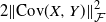 $ 2\|\text{Cov}(X,Y)\|_{\mathcal{F}}^2 $
thanks to Lemma 3.1 (Isserlis), and so problem (2.1) in that case becomes
 $\sup_{X \sim T_0\#\mu, Y \sim T_1\#\nu} 4\|\text{Cov}(X,Y)\|_{\mathcal{F}}^2$
. Applying Lemma 3.2, we can exhibit a Gaussian optimal plan
 $ \tilde{\pi}^* \in \Pi(T_0\#\mu,T_1\#\nu ) $
with covariance matrix
 $ \Sigma $
of the form
 \begin{equation*} \Sigma = \begin{pmatrix} D_0 & \quad K^* \\[4pt] K^{*\top} & \quad D_1 \end{pmatrix},\end{equation*}
with
 \begin{equation*} K^* = \begin{pmatrix} \tilde{I}_n\big(D_0^{(n)}\big)^{1/2}D_1^{1/2} \\[5pt] 0_{m-n,n} \end{pmatrix}.\end{equation*}
Thus, applying Lemma 3.4, it follows directly that
 $ \tilde{\pi}^* $
is of the form
 $ (I_m,\tilde{T})\#T_0\#\mu $
, with
 $ \tilde{T} $
linear of the form
 $\tilde{T}(x) = Ax$
for all
 $x \in \mathbb{R}^m$
, with A of the form
 $A = \Big(\tilde{I}_nD_1^{{1}/{2}}\big(D_0^{(n)}\big)^{-{1}/{2}} \quad 0_{n,m-n} \Big)$
. Then, we can deduce the form of the optimal Gaussian plan
 $ \pi^* \in \Pi(\mu,\nu) $
:
 \begin{align*} \pi^* &= (T_0^{-1},T_1^{-1})\#\tilde{\pi}^* \\ &= (T_0^{-1},T_1^{-1})\#(I_m,\tilde{T})\#T_0\#\mu \\ &= (I_m,T_1^{-1}\#\tilde{T}\#T_0)\#\mu = (I_m,T)\#\mu ,\end{align*}
where T is affine of the form, for all
 $x \in \mathbb{R}^m$
,
 $T(x) = T_1^{-1}\circ\tilde{T}\circ T_0(x) = m_1 + P_1AP_0^\top (x - m_0)$
. Moreover, using Lemmas 2.2 and 3.2, it follows that
 \begin{align*} & GGW_2^2(\mu,\nu) = C_{\mu,\nu} - 16\sup_{X \sim T_0\#\mu, Y \sim T_1\#\nu} \|\text{Cov}(X,Y)\|_{\mathcal{F}}^2 \\ & = 8\text{tr}(D_0^2) + 4(\text{tr}(D_0))^2 + 8\text{tr}(D_1^2) + 4(\text{tr}(D_1))^2 - 4\text{tr}(D_0)\text{tr}(D_1) - 16\text{tr}(D_0^{(n)}D_1) \\ & = 4({tr}(D_0) - {tr}(D_1))^2 + 8{tr}\big((D_0^{(n)} - D_1)^2\big) + 8\big({tr}(D_0^2) - \text{tr}((D_0^{(n)})^2)\big). \end{align*}
4.1. Link with Gromov–Monge
The previous result generalizes [Reference Vayer25, Theorem 4.2.6], which studies the solutions of the linear Gromov–Monge problem between Gaussian distributions,
 \begin{equation*} \inf_{T \# \mu=\nu,\, \text{T linear}} \int \int \big(\|x - x^{\prime}\|^2_{\mathbb{R}^m} - \|T(x) - T(x^{\prime})\|^2_{\mathbb{R}^n}\big)^2 \, \textrm{d}\mu(x) \, \textrm{d}\mu(x^{\prime}).\end{equation*}
Indeed, solutions of this equation necessarily provide Gaussian transport plans
 $\pi = (I_m,T)\#\mu$
if T is linear. Conversely, Theorem 4.1 shows that restricting the optimal plan to be Gaussian in Gromov–Wasserstein between two Gaussian distributions yields an optimal plan of the form
 $\pi = (I_m,T)\#\mu$
with a linear T, whatever the dimensions m and n of the two Euclidean spaces.
4.2. Link with PCA
We can easily draw connections between
 $ GGW_2^2 $
and PCA. Indeed, we can remark that the optimal plan can be derived by performing PCA on both distributions
 $ \mu $
and
 $ \nu $
in order to obtain distributions
 $ \tilde{\mu} $
and
 $ \tilde{\nu} $
with zero mean vectors and diagonal covariance matrices with eigenvalues in decreasing order (
 $\tilde{\mu} = T_0\#\mu$
and
 $\tilde{\nu} = T_1\#\nu$
), then by keeping only the n first components in
 $ \tilde{\mu} $
, and finally by deriving the optimal transport plan which achieves
 $ W_2^2 $
between the obtained truncated distribution and
 $ \tilde{\nu} $
. In other terms, writing
 $ P_n\,:\, \mathbb{R}^m \rightarrow \mathbb{R}^n $
as the linear mapping which, for
 $ x \in \mathbb{R}^m $
, keeps only its n first components (n-frame), and
 $ T_{W_2} $
as the optimal transport map such that
 $ \pi_{W_2} = (I_n,T_{W_2})\#P_n\#\tilde{\mu} $
achieves
 $ W_2(P_n\#\tilde{\mu},\tilde{\nu}) $
, it follows that the optimal plan
 $ \pi_{GGW_2} $
which achieves
 $GGW_2(\tilde{\mu},\tilde{\nu}) $
can be written as
 $\pi_{GGW_2} = (I_m,\tilde{I}_n\#T_{W_2}\#P_n)\#\tilde{\mu}$
, where, with an abuse of notation, we write
 $I_m$
(resp.
 $\tilde{I}_n$
) as the map on
 $\mathbb{R}^m$
(resp.
 $\mathbb{R}^n$
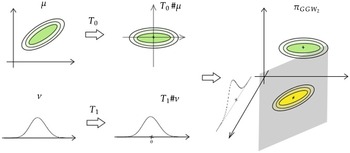
) represented by the similarly denoted matrix. An example of
 $ \pi_{GGW_2} $
can be found in Figure 1 when
 $ m = 2 $
and
 $ n = 1 $
.
Transport plan
 $ \pi_{GGW_2} $
solution of problem (4.1) with
 $ m = 2 $
and
 $ n =1 $
. In this case,
 $ \pi_{GGW_2} $
is the degenerate Gaussian distribution supported by the affine plane of equation
 $ y = T_{W_2}(x) $
, where
 $ T_{W_2} $
is the classic
 $ W_2 $
optimal transport map when the distributions are rotated and centered first.

4.3. Case of equal dimensions
When
 $ m = n $
, the optimal plan
 $ \pi_{GGW_2} $
which achieves
 $ GGW_2(\mu,\nu) $
is closely related to the optimal transport plan
 $ \pi_{W_2} = (I_m,T_{W_2})\#T_0\#\mu $
. Indeed,
 $ \pi_{GGW_2} $
can be derived simply by applying the transformations
 $ T_0 $
and
 $ T_1 $
to
 $ \mu $
and
 $ \nu$
respectively, then by computing
 $ \pi_{W_2} $
between
 $ T_0\#\mu $
and
 $ T_1\#\nu $
, and finally by applying the inverse transformations
 $ T_0^{-1} $
and
 $ T_1^{-1} $
. In other terms,
 $ \pi_{GGW_2} $
can be written as
 $\pi_{GGW_2} = (I_m,T_1^{-1}\#\tilde{I}_n\#T_{W_2}\#T_0)\#\mu$
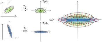
. An example of transport between two Gaussian measures in dimension 2 is shown in Figure 2.
Solution of (4.1) between two Gaussians measures in dimension 2. First the distributions are centered and rotated. Then a classic
 $ W_2 $
transport is applied between the two aligned distributions.

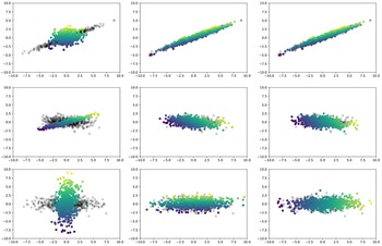
As illustrated in Figure 3, the
 $ GGW_2 $
optimal transport map
 $ T_{GGW_2} $
defined in (4.2) is not equivalent to the
 $ W_2$
optimal transport map
 $ T_{W_2} $
defined in (1.3), even when the dimensions m and n are equal. More precisely, if
 $ \Sigma_0 $
and
 $ \Sigma_1 $
can be diagonalized in the same orthonormal basis with eigenvalues in the same order (decreasing or increasing), then
 $ T_{W_2} $
and
 $ T_{GGW_2} $
are equivalent (top of Figure 3). On the other hand, if
 $ \Sigma_0 $
and
 $ \Sigma_1 $
can be diagonalized in the same orthonormal basis but with eigenvalues not in the same order,
 $ T_{W_2} $
and
 $ T_{GGW_2} $
will have very different behaviors (bottom of Figure 3). Between those two extreme cases, we can say that the closer the columns of
 $ P_0 $
are to being collinear with the columns of
 $ P_1 $
(with the eigenvalues in decreasing order), the more
 $ T_{W_2} $
and
 $ T_{GGW_2} $
will tend to have similar behaviors (middle of Figure 3).
Comparison between
 $W_2 $
and
 $ GGW_2 $
mappings between empirical distributions. Left: Two-dimensional source distribution (colored) and target distribution (transparent). Middle: Resulting mapping of Wasserstein
 $ T_{W_2} $
. Right: Resulting mapping of Gaussian Gromov–Wasserstein
 $ T_{GGW_2} $
. The colors are added in order to visualize where each sample has been sent.

4.4. Link with Gromov–Wasserstein with inner product as cost function
If
 $ \mu $
and
 $ \nu $
are centered Gaussian measures, let us consider the problem
 \begin{equation} GW_2^2(\langle \cdot,\cdot \rangle_m,\langle \cdot,\cdot \rangle_n,\mu,\nu) = \inf_{\pi \in \Pi(\mu,\nu)} \int \int (\langle x,x^{\prime}\rangle_m - \langle y,y^{\prime}\rangle_n)^2 \, \textrm{d}\pi(x,y) \, \textrm{d}\pi(x^{\prime},y^{\prime}).\end{equation}
Notice that the above problem is not restricted to Gaussian plans, but the following proposition shows that in fact its solution is Gaussian.
Proposition 4.2. Suppose
 $ m \leq n $
. Let
 $\mu = \mathcal{N}(0,\Sigma_0) $
and
 $ \nu = \mathcal{N}(0,\Sigma_1) $
be two centered Gaussian measures respectively on
 $ \mathbb{R}^m $
and
 $ \mathbb{R}^n $
. Then the solution of problem (4.1) exhibited in Theorem 4.1 is also a solution of problem (4.4).
Proof. The proof of this proposition is a direct consequence of Lemma 2.2; indeed, applying it with
 $ a = 0 $
,
 $ b = 0 $
, and
 $ c = 1 $
, it follows that problem (4.4) is equivalent to
 $\sup_{\pi \in \Pi(\mu,\nu)} \big\|\int xy^\top \, \textrm{d}\pi(x,y)\big\|_{\mathcal{F}}^2$
. Since
 $ \mu $
and
 $ \nu $
are centered, it follows that problem (4.4) is equivalent to
 $\sup_{X \sim \mu, Y \sim \nu} \|\text{Cov}(X,Y)\|_{\mathcal{F}}^2$
. Applying Lemma 3.2, it follows that the solution exhibited in Theorem 4.1 is also a solution of problem (4.4).
5. Tightness of the bounds and particular cases
5.1. Bound on the difference
Proposition 5.1. Suppose, without loss of generality, that
 $ n \leq m $
. If
 $ \mu = \mathcal{N}(m_0,\Sigma_0) $
and
 $ \nu = \mathcal{N}(m_1,\Sigma_1)$
, then
 \begin{equation*} GGW_2^2(\mu,\nu) - LGW_2^2(\mu,\nu) \leq 8\|\Sigma_0\|_{\mathcal{F}}\|\Sigma_1\|_{\mathcal{F}}\bigg(1 - \frac{1}{\sqrt{m}\,}\bigg). \end{equation*}
To prove this proposition we will use the following technical result (the proof is postponed to Appendix A).
Lemma 5.1. Let
 $ u \in \mathbb{R}^m $
and
 $ v \in \mathbb{R}^m $
be two unit vectors with non-negative coordinates ordered in decreasing order. Then
 $u^\top v \geq {1}/{\sqrt{m}}$
, with equality if
 $ u = ({1}/{\sqrt{m}},{1}/{\sqrt{m}},\dots)^\top $
and
 $ v = (1,0,\dots)^\top $
.
Proof of Proposition 5.1.By subtracting (3.1) from (4.3), it follows that
 \begin{align} GGW_2^2(\mu,\nu) - LGW_2^2(\mu,\nu) &= 8\big(\|D_0\|_{\mathcal{F}}\|D_1\|_{\mathcal{F}} - \text{tr}(D_0^{(n)}D_1)\big) \nonumber \\ &= 8\big(\|D_0\|_{\mathcal{F}}\|D_1^{[m]}\|_{\mathcal{F}} - \text{tr}(D_0D_1^{[m]})\big), \end{align}
where
 $ D_1^{[m]} = \big( \begin{smallmatrix} D_1 & 0 \\ 0 & 0 \end{smallmatrix} \big) \in \mathbb{R}^{m \times m} $
. Writing
 $ \alpha \in \mathbb{R}^m $
and
 $ \beta \in \mathbb{R}^m $
as the vectors of eigenvalues of
 $ D_0 $
and
 $ D_1^{[m]} $
, it follows that
 $GGW_2^2(\mu,\nu) - LGW_2^2(\mu,\nu) = 8\big(\|\alpha\|\|\beta\| - \alpha^\top \beta\big) = 8\|\alpha\|\|\beta\|(1 - u^\top v)$
, where
 $ u = {\alpha}/{\|\alpha\|} $
and
 $ v = {\beta}/{\|\beta\|} $
. Applying Lemma 5.1, we get directly that
 \begin{align*} GGW_2^2(\mu,\nu) - LGW_2^2(\mu,\nu) & \leq 8\|D_0\|_{\mathcal{F}}\|D_1^{[m]}\|_{\mathcal{F}}\bigg(1 - \frac{1}{\sqrt{m}\,}\bigg) \\ & = 8\|\Sigma_0\|_{\mathcal{F}}\|\Sigma_1\|_{\mathcal{F}}\bigg(1 - \frac{1}{\sqrt{m}\,}\bigg). \end{align*}
The difference between
 $ GGW_2^2(\mu,\nu) $
and
 $ LGW_2^2(\mu,\nu) $
can be seen as the difference between the right and left terms of the Cauchy–Schwarz inequality applied to the two vectors of eigenvalues
 $ \alpha \in \mathbb{R}^m $
and
 $ \beta \in \mathbb{R}^m $
. The difference is maximized when the vectors
 $ \alpha $
and
 $ \beta $
are the least collinear possible. This happens when the eigenvalues of
 $ D_0 $
are all equal and
 $ n = 1 $
or
 $ \nu $
is degenerate of true dimension 1. On the other hand, this difference is null when
 $ \alpha $
and
 $ \beta $
are collinear. Between those two extremal cases, we can say that the difference between
 $ GGW_2^2(\mu,\nu) $
and
 $ LGW_2^2(\mu,\nu) $
will be relatively small if the last
 $ m - n $
eigenvalues
 $ D_0 $
are small compared to the n first eigenvalues, and if the n first eigenvalues are close to being proportional to the eigenvalues of
 $ D_1 $
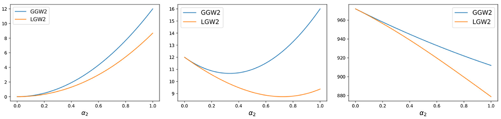
. An example in the case where
 $ m = 2 $
and
 $ n = 1$
can be found in Figure 4.
Plot of
 $ GGW_2^2(\mu,\nu) $
and
 $ LGW_2^2(\mu,\nu) $
as a function of
 $ \alpha_2 $
for
 $ \mu = \mathcal{N}(0,\text{diag}(\alpha)) $
,
 $ \nu = \mathcal{N}(0,\beta_1) $
,
 $ \alpha = (\alpha_1,\alpha_2)^\top $
, for
 $(\alpha_1,\beta_1) = (1,1) $
(left),
 $ (\alpha_1,\beta_1) = (1,2) $
(middle), and
 $ (\alpha_1,\beta_1) = (1,10) $
(right). We can easily compute using (4.3) and (3.1) that
 $ GGW_2^2(\mu,\nu) = 12\alpha_2^2 + 8\alpha_2(\alpha_1 - \beta_1) + 12(\alpha_1 - \beta_1)^2 $
and
 $ LGW_2^2(\mu,\nu) = 12\alpha_2^2 + 8\alpha_2(\alpha_1 - \beta_1) - 4\big[\alpha_2^2 + \alpha_1^2\big]^{1/2}\beta_1 + 12(\alpha_1 - \beta_1)^2 + 8\alpha_1\beta_1$
.

5.2. Explicit case
As seen before, the difference between
 $ GGW_2^2(\mu,\nu) $
and
 $ LGW_2^2(\mu,\nu) $
, with
 $ \mu = \mathcal{N}(m_0,\Sigma_0) $
and
 $ \nu = \mathcal{N}(m_1,\Sigma_1) $
, is null when the two vectors of eigenvalues of
 $ \Sigma_0 $
and
 $\Sigma_1 $
(sorted in decreasing order) are collinear. When we suppose
 $ \Sigma_0 $
non-singular, it implies that
 $ m = n $
and that the eigenvalues of
 $ \Sigma_1 $
are proportional to the eigenvalues of
 $ \Sigma_0 $
(rescaling). This case includes the more particular case where
 $ m = n = 1$
. In that case,
 $ \mu = \mathcal{N}(m_0,\sigma_0^2) $
and
 $ \nu = \mathcal{N}(m_1,\sigma_1^2) $
, because
 $ \sigma_1 $
is always proportional to
 $ \sigma_0 $
.
Proposition 5.2. Suppose
 $ m = n $
. Let
 $ \mu = \mathcal{N}(m_0,\Sigma_0) $
and
 $ \nu = \mathcal{N}(m_1,\Sigma_1) $
be two Gaussian measures on
 $ \mathbb{R}^m = \mathbb{R}^n $
. Let
 $ P_0,D_0 $
and
 $ P_1,D_1 $
be the respective diagonalizations of
 $\Sigma_0\ (= P_0D_0P_0^\top )$
and
 $ \Sigma_1\ (=P_1D_1P_1^\top ) $
which sort the eigenvalues in non-increasing order. Suppose
 $ \Sigma_0 $
is non-singular and that a scalar
 $ \lambda \geq 0 $
exists such that
 $ D_1 = \lambda D_0 $
. In that case,
 $ GW_2^2(\mu,\nu) = GGW_2^2(\mu,\nu) = LGW_2^2(\mu,\nu) $
and the problem admits a solution of the form
 $ (I_m, T)\#\mu$
with T affine of the form, for all
 $x \in \mathbb{R}^m$
,
 \begin{equation} T(x) = m_1 + \sqrt{\lambda} P_1\tilde{I}_mP_0^\top (x - m_0), \end{equation}
where
 $ \tilde{I}_m $
is of the form
 $ {diag}((\pm 1)_{i \leq m}) $
. Moreover,
 \begin{equation} GW_2^2(\mu,\nu) = (\lambda - 1)^2\left(4({tr}(\Sigma_0))^2 + 8\|\Sigma_0\|_{\mathcal{F}}^2\right). \end{equation}
Proof. From (5.1),
 $GGW_2^2(\mu,\nu) - LGW2^2(\mu,\nu) = 8(\|D_0\|_{\mathcal{F}}\|D_1\|_{\mathcal{F}} - \text{tr}(D_0D_1))$
. Writing
 $ \alpha \in \mathbb{R}^m $
and
 $ \beta \in \mathbb{R}^m $
for the eigenvalue vectors of
 $ D_0 $
and
 $ D_1 $
, it follows that
 $GGW_2^2(\mu,\nu) - LGW2^2(\mu,\nu) = 8(\|\alpha\|\|\beta\| - \alpha^\top \beta)$
. Since
 $ \lambda \geq 0 $
exists such that
 $ D_1 = \lambda D_0 $
, we have
 $ \beta = \lambda \alpha $
, and so
 $ \alpha^\top \beta = \|\alpha\|\|\beta\| $
. Thus,
 $ GGW_2^2(\mu,\nu) - LGW_2^2(\mu,\nu) = 0 $
and, using Proposition 4.1, we get that
 $ GW_2^2(\mu,\nu) = GGW_2^2(\mu,\nu) = LGW^2_2(\mu,\nu) $
. We get (5.2) and (5.3) by simply reinjecting in (4.2) and (4.3).
Corollary 5.1. Let
 $ \mu = \mathcal{N}(m_0,\sigma_0^2) $
and
 $ \nu = \mathcal{N}(m_1,\sigma_1^2) $
be two Gaussian measures on
 $ \mathbb{R} $
. Then
 $GW_2^2(\mu, \nu) = 12\left(\sigma_0^2 - \sigma_1^2\right)^2$
, and the optimal transport plan
 $ \pi^* $
has the form
 $ (I_1,T)\#\mu $
, with T affine of the form, for all
 $x \in \mathbb{R}$
,
 $T(x) = m_1 \pm ({\sigma_1}/{\sigma_0})(x - m_0)$
. Thus, the solution of
 $ W^2_2(\mu,\nu) $
is also a solution of
 $ GW_2^2(\mu,\nu) $
.
5.3. Case of degenerate measures
In all the results described above, we have supposed
 $ \Sigma_0 $
to be non-singular, which means that
 $ \mu $
is not degenerate. Yet, if
 $ \Sigma_0 $
is not full rank, we can easily extend the previous results thanks to the following proposition.
Proposition 5.3. Let
 $ \mu = \mathcal{N}(0,D_0) $
and
 $ \nu = \mathcal{N}(0,D_1) $
be two centered Gaussian measures on
 $ \mathbb{R}^m $
and
 $ \mathbb{R}^n $
with diagonal covariance matrices
 $ D_0 $
and
 $ D_1 $
with eigenvalues in decreasing order. We denote by
 $ r = \textrm{rk}(D_0)$
the rank of
 $ D_0 $
, and we suppose that
 $ r < m $
. Let us define
 $ P_r = \big( I_r \quad 0_{r,m-r} \big) \in \mathbb{R}^{r \times m} $
. Then
 $ GW_2^2(\mu,\nu) = GW_2^2(P_r\#\mu,\nu) $
,
 $ GGW_2^2(\mu,\nu) = GGW_2^2(P_r\#\mu,\nu)$
, and
 $ LGW_2^2(\mu,\nu) = LGW_2^2(P_r\#\mu,\nu) $
.
Proof. For
 $ r < m $
, we denote by
 $ \Gamma_r(\mathbb{R}^m) $
the set of vectors
 $ x = (x_1,\dots,x_m)^\top $
of
 $ \mathbb{R}^m $
such that
 $ x_{r + 1} = \dots = x_{m} = 0 $
. For
 $ \pi \in \Pi(\mu,\nu) $
, we can remark that for any Borel set
 $ A \subset \mathbb{R}^m \setminus \Gamma_r(\mathbb{R}^m) $
, and any Borel set
 $ B \subset \mathbb{R}^n $
, we have
 $ \pi(A,B) = 0 $
and so
 \begin{align*} & GW_2^2(\mu,\nu) = \inf_{\pi \in \Pi(\mu,\nu)}\int_{\mathbb{R}^m \times \mathbb{R}^n}\int_{\mathbb{R}^m \times \mathbb{R}^n}\big(\|x -x^{\prime}\|^2_{\mathbb{R}^m} - \|y -y^{\prime}\|^2_{\mathbb{R}^m}\big)^2 \, \textrm{d}\pi(x,y) \, \textrm{d}\pi(x^{\prime},y^{\prime}) \\ & = \inf_{\pi \in \Pi(\mu,\nu)}\int_{\Gamma_r(\mathbb{R}^m) \times \mathbb{R}^n}\int_{\Gamma_r(\mathbb{R}^m) \times \mathbb{R}^n}\big(\|x -x^{\prime}\|^2_{\mathbb{R}^m} - \|y -y^{\prime}\|^2_{\mathbb{R}^m}\big)^2 \, \textrm{d}\pi(x,y) \, \textrm{d}\pi(x^{\prime},y^{\prime}) \\ & = \inf_{\pi \in \Pi(\mu,\nu)}\int_{\Gamma_r(\mathbb{R}^m)\times\mathbb{R}^n}\int_{\Gamma_r(\mathbb{R}^m)\times\mathbb{R}^n}\big(\|P_r(x -x^{\prime})\|^2_{\mathbb{R}^r} - \|y -y^{\prime}\|^2_{\mathbb{R}^m}\big)^2 \, \textrm{d}\pi(x,y) \, \textrm{d}\pi(x^{\prime},y^{\prime}) .\end{align*}
Now, observe that, for
 $\pi \in \Pi(\mu,\nu)$
,
 $(P_r,I_n)\#\pi \in \Pi(P_r\#\mu,\nu)$
. It follows that
 \begin{align*} GW_2^2(\mu,\nu) &\le \inf_{\pi \in \Pi(P_r\#\mu,\nu)}\int_{\mathbb{R}^r\times\mathbb{R}^n}\int_{\mathbb{R}^r\times\mathbb{R}^n}\big(\|x -x^{\prime}\|^2_{\mathbb{R}^r} - \|y -y^{\prime}\|^2_{\mathbb{R}^m}\big)^2 \, \textrm{d}\pi(x,y) \, \textrm{d}\pi(x^{\prime},y^{\prime}) \\ &= GW_2^2(P_r\#\mu,\nu).\end{align*}
Conversely, since
 $\mu$
has no mass outside of
 $\Gamma_r(\mathbb{R}^m)$
,
 $P_r^\top \#P_r\#\mu = \mu$
, which implies that for
 $\pi \in \Pi(P_r\#\mu,\nu)$
,
 $(P_r^\top ,I_n)\#\pi \in \Pi(\mu,\nu)$
. It follows that
 \begin{align*} & GW_2^2(P_r\#\mu,\nu) \\ & = \inf_{\pi \in \Pi(P_r\#\mu,\nu)}\int_{\mathbb{R}^r\times\mathbb{R}^n}\int_{\mathbb{R}^r\times\mathbb{R}^n}\big(\|x -x^{\prime}\|^2_{\mathbb{R}^r} - \|y -y^{\prime}\|^2_{\mathbb{R}^m}\big)^2 \, \textrm{d}\pi(x,y) \, \textrm{d}\pi(x^{\prime},y^{\prime}) \\ & = \inf_{\pi \in \Pi(P_r\#\mu,\nu)}\int_{\mathbb{R}^r\times\mathbb{R}^n}\int_{\mathbb{R}^r\times\mathbb{R}^n}\big(\|P_r^\top (x -x^{\prime})\|^2_{\mathbb{R}^r} - \|y -y^{\prime}\|^2_{\mathbb{R}^m}\big)^2 \, \textrm{d}\pi(x,y) \, \textrm{d}\pi(x^{\prime},y^{\prime}) \\ & \le \inf_{\pi \in \Pi(\mu,\nu)}\int_{\mathbb{R}^m\times\mathbb{R}^n}\int_{\mathbb{R}^m\times\mathbb{R}^n}\big(\|x -x^{\prime}\|^2_{\mathbb{R}^r} - \|y -y^{\prime}\|^2_{\mathbb{R}^m}\big)^2 \, \textrm{d}\pi(x,y) \, \textrm{d}\pi(x^{\prime},y^{\prime}) \\ & \le GW_2^2(\mu,\nu) .\end{align*}
The exact same reasoning can be made in the case of
 $ GGW_2 $
. Moreover, it can be easily seen when looking at (3.1) that
 $ LGW_2^2(\mu,\nu) = LGW_2^2(P_r\#\mu,\nu) $
.
Thus, when
 $ \Sigma_0 $
is not full rank, we can apply Proposition 5.3 and consider directly the Gromov–Wasserstein distance between the projected (non-degenerate) measure
 $ P_r\#\mu $
on
 $ \mathbb{R}^r $
and
 $ \nu $
, and so Proposition 4.1 still holds when
 $ \mu $
is degenerate.
In the case of
 $ GGW_2 $
, an explicit optimal transport plan can still be exhibited. In the following, we denote by
 $ r_0 $
and
 $ r_1 $
the ranks of
 $ \Sigma_0 $
and
 $ \Sigma_1 $
, and we suppose without loss of generality that
 $ r_0 \geq r_1 $
, but this time not necessarily that
 $ m \geq n $
. If
 $ \mu = \mathcal{N}(m_0,\Sigma_0) $
and
 $ \nu = \mathcal{N}(m_1,\Sigma_1) $
are two Gaussian measures on
 $ \mathbb{R}^m $
and
 $ \mathbb{R}^n $
, and
 $ (P_0,D_0) $
and
 $ (P_1,D_1) $
are the respective diagonalizations of
 $ \Sigma_0\ (= P_0D_0P_0^\top ) $
and
 $ \Sigma_1\ (= P_1D_1P_1^\top ) $
which sort the eigenvalues in decreasing order, an optimal transport plan which achieves
 $ GGW_2(\mu,\nu) $
is of the form
 $ \pi^* = (I_m,T)\#\mu $
with, for all
 $x \in \mathbb{R}^m$
,
 $T(x) = m_1 + P_1AP_0^\top (x - m_0)$
, where
 $ A \in \mathbb{R}^{n \times m} $
is of the form
 \begin{equation*} A = \begin{pmatrix} \tilde{I}_{r_1}(D_1^{(r_1)})^{{1}/{2}}(D_0^{(r_1)})^{-{1}/{2}} & \quad 0_{r_1,m - r_1} \\[5pt] 0_{n - r_1, r_1} & \quad 0_{n - r_1, m - r_1} \end{pmatrix}, \end{equation*}
where
 $ \tilde{I}_{r_1} $
is any matrix of the form
 $ \text{diag}((\pm 1)_{i \leq r_1}) $
.
6. Behavior of the empirical solution
In this section we perform a simple experiment to illustrate the behavior of the solution of the Gromov–Wasserstein problem. In this experiment, we draw independently k samples
 $ (X_j)_{j \leq k} $
and
 $ (Y_i)_{i \leq k} $
from, respectively,
 $ \mu = \mathcal{N}(0,\text{diag}(\alpha))$
and
 $ \nu = \mathcal{N}(0,\text{diag}(\beta)) $
, with
 $ \alpha \in \mathbb{R}^m $
and
 $ \beta \in \mathbb{R}^n $
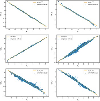
. Then we compute the Gromov–Wasserstein distance between the two histograms X and Y with the algorithm proposed in [Reference Peyré, Cuturi and Solomon19] using the Python Optimal Transport library (accessible at https://pythonot.github.io/index.html). In Figure 5, we plot the first coordinates of the samples
 $ Y_i $
as a function of the the first coordinate of the samples
 $ X_j $
they have been assigned to by the algorithm (blue dots). We also draw the line
 $ y = \pm\sqrt{\beta}x $
to compare with the theorical solution of the Gaussian restricted problem (orange line) for
 $ k = 2000 $
,
 $ \alpha = (1,0.1)^\top $
, and
 $ \beta = 2 $
(top left);
 $ k = 2000 $
,
 $ \alpha = (1,0.1)^\top $
, and
 $ \beta = (2,0.3)^\top $
(top right);
 $ k = 2000 $
,
 $ \alpha = (1,0.1,0.01)^\top $
, and
 $ \beta = 2 $
(middle left);
 $ k = 7000 $
,
 $ \alpha = (1,0.3) $
, and
 $\beta = 2$
(middle right);
 $ k = 7000 $
,
 $ \alpha = (1,0.1)^\top $
, and
 $ \beta = (2,1)^\top $
(bottom left); and
 $ k = 7000 $
,
 $ \alpha = (1,0.3,0.1)$
, and
 $ \beta = 2 $
(bottom right). Observe that the empirical solution seems to be behaving in exactly the same way as the theoretical solution exhibited in Theorem 4.1 as soon as
 $ \alpha $
and
 $ \beta $
are close to being collinear. However, when
 $ \alpha $
and
 $ \beta $
are further away from collinearity, determining the behavior of the empirical solution becomes more complex. Solving Gromov–Wasserstein numerically, even approximately, is a particularly hard task, therefore we cannot conclude whether the empirical solution does not behave in the same way as the theorical solution exhibited in Theorem 4.1 or whether the algorithm has not converged in these more complex cases. This second assumption seems to be more likely because it seems that increasing the number of points k reduces the gap between the blue dots and the orange line. Thus, we conjecture that the optimal plan which achieves
 $ GGW_2(\mu,\nu) $
is also a solution of the non-restricted problem
 $ GW_2(\mu,\nu) $
, and that
 $ GW_2(\mu,\nu) = GGW_2(\mu,\nu) $
.
Plot of the first coordinate of samples
 $ Y_i $
as a function of the the first coordinate of their assigned samples
 $ X_j $
(blue dots) and the line
 $ y = \pm\sqrt{\beta}x $
(orange line) for
 $ k = 2000 $
,
 $ \alpha = (1,0.1)^\top $
, and
 $ \beta = 2 $
(top left);
 $ k = 2000 $
,
 $ \alpha = (1,0.1)^\top $
, and
 $ \beta = (2,0.3)^\top $
(top right);
 $ k = 2000 $
,
 $ \alpha = (1,0.1,0.01)^\top $
, and
 $ \beta = 2 $
(middle left);
 $ k = 7000 $
,
 $ \alpha = (1,0.3) $
, and
 $\beta = 2$
(middle right);
 $ k = 7000 $
,
 $ \alpha = (1,0.1)^\top $
, and
 $ \beta = (2,1)^\top $
(bottom left); and
 $ k = 7000 $
,
 $ \alpha = (1,0.3,0.1)$
, and
 $ \beta = 2 $
(bottom right).

7. Conclusion
We have exhibited lower and upper bounds for the Gromov–Wasserstein distance (with a squared ground distance) between Gaussian measures living on different Euclidean spaces. We have also studied the tightness of the provided bounds, both theoretically and numerically. The upper bound is obtained through the study of the problem with the additional restriction that the optimal plan itself is Gaussian. We have shown that this particular case has a very simple closed-form solution, which can be described as first performing PCA on both distributions and then deriving the optimal linear plan between these aligned distributions. We conjecture that the linear solution exhibited when adding this restriction might also be the solution of the unconstrained problem.
Appendix A. Proofs of the lemmas
A.1. Proof of Lemma 3.2
Proof. The proof is inspired from the proof of (1.2) as provided in [Reference Givens13]. We want to maximize
 $ \text{tr}(K^\top K) $
with the constraint that
 $ \Sigma $
is semi-definite positive. Let
 $ S = \Sigma_1 - K^\top \Sigma_0^{-1}K $
(Schur complement); problem (3.2) can be written as
 $\min_{S \in S^+_n(\mathbb{R}) } - \text{tr}(K^\top K)$
. For a given S, the set of feasible K is the set of K such that
 $ K^\top \Sigma_0^{-1}K = \Sigma_1 - S $
. Since
 $ \Sigma_0 \in S^{++}_m(\mathbb{R}) $
,
 $ K^\top \Sigma_0^{-1}K \in S^{+}_n(\mathbb{R}) $
and so
 $ \Sigma_1 - S \in S^{+}_n(\mathbb{R}) $
. We denote by r the rank of
 $ K^\top \Sigma_0^{-1}K $
. We can observe that
 $ r \leq n \leq m$
, where the left-hand inequality follows from the fact that
 $ \text{rk}(AB) \leq \min\{\text{rk}(A),\text{rk}(B)\}$
. Then,
 $ \Sigma_1 - S $
can be diagonalized,
 \begin{equation}\Sigma_1 - S = K^\top \Sigma_0^{-1}K = U\Lambda^2 U^\top = U_r\Lambda^2_rU_r^\top ,\end{equation}
with
 $ \Lambda^2 = \text{diag}(\lambda_1^2,\ldots,\lambda_r^2,0,\ldots,0)$
,
 $ \Lambda_r^2 = \text{diag}(\lambda_1^2,\ldots,\lambda_r^2) $
, and
 $ U_r \in \mathbb{V}_r(\mathbb{R}^n) \,:\!=\, \{M \in \mathbb{R}^{n \times r} \mid M^\top M = I_r \} $
(Stiefel manifold [Reference James15]) such that
 $ U = \big( U_r \quad U_{n-r} \big)$
. From (A.1), we can deduce that
 $(\Sigma_0^{-{1}/{2}}KU_r\Lambda_r^{-1})^\top \Sigma_0^{-{1}/{2}}KU_r\Lambda_r^{-1} = I_r$
. We can set
 $ B_r = \Sigma_0^{-{1}/{2}}KU_r\Lambda_r^{-1} $
such that
 $ B_r \in\mathbb{V}_r(\mathbb{R}^m) $
, and deduce that
 $KU_r = \Sigma_0^{{1}/{2}}B_r\Lambda_r$
. Moreover, since
 $ U_{m-r}^\top K^\top \Sigma_0^{-1}KU_{m-r} = 0 $
and
 $\Sigma_0 \in S_m^{++}(\mathbb{R}) $
, it follows that
 $ KU_{n-r} = 0 $
and so
 \begin{equation}K = KUU^\top = KU_rU_r^\top = \Sigma_0^{\frac{1}{2}}B_r\Lambda_rU_r^\top .\end{equation}
We can write
 $ \text{tr}(K^\top K) $
as a function of
 $ B_r$
:
 \begin{equation*}\text{tr}(K^\top K) =\text{tr}(U_r\Lambda_rB_r^\top \Sigma_0B_r\Lambda_rU_r^\top ) = \text{tr}(U_r^\top U_r\Lambda_rB_r^\top \Sigma_0B_r\Lambda_r) = \text{tr}(\Lambda^2_rB_r^\top \Sigma_0B_r) .\end{equation*}
Thus, for a given S, the set of K such that
 $ K^\top \Sigma_0^{-1}K = \Sigma_1 - S $
is parametrized by the r-frame
 $ B_r $
. We want to find
 $ B_r $
which maximizes
 $ \text{tr}(K^\top K) $
for a given S. This problem can be rewritten as
 \begin{equation} \min_{B_r \in \mathbb{V}_r(\mathbb{R}^m)} - \text{tr}\big(\Lambda^2_rB_r^\top \Sigma_0B_r\big).\end{equation}
The following is an adaptation of the proof of [Reference Anstreicher and Wolkowicz2, Proposition (3.1)] for when
 $ B_r $
is not a squared matrix. The Lagrangian of problem (A.3) can be written as
 $\mathcal{L}(B_r,C) = -\text{tr}(\Lambda^2_rB_r^\top \Sigma_0B_r) + \text{tr}(C(B_r^\top B_r - I_r))$
, where
 $ C \in S_r(\mathbb{R}) $
is the Lagrange multiplier associated with the constraint
 $ B_r^\top B_r = I_r $
(C is symmetric because
 $ B_r^\top B_r - I_r $
is symmetric). We can then derive the first-order condition
 $-2\Sigma_0B_r\Lambda_r^2 + 2B_rC = 0$
, or, equivalently,
 $\Sigma_0B_r\Lambda_r^2B_r^\top = B_rCB_r^\top $
. Since
 $ C \in S_r(\mathbb{R}) $
,
 $ B_rCB_r^\top \in S_m(\mathbb{R}) $
and
 $ \Sigma_0B_r\Lambda_r^2B_r^\top \in S_m(\mathbb{R}) $
. We can deduce that
 $ \Sigma_0 $
and
 $ B_r\Lambda_rB_r^\top $
commute. Moreover, since
 $ \Sigma_0 $
and
 $ B_r\Lambda_r^2B_r^\top $
are both symmetric, they can be diagonalized in the same basis. Since
 $ B_r \in \mathbb{V}_r(\mathbb{R}^m) $
, it can be seen as the r first vectors of an orthogonal basis of
 $ \mathbb{R}^m $
. It means there exists a matrix
 $ B_{m-r} $
such that
 $B_r\Lambda_r^2B_r^\top = B\Lambda_m^2B^\top $
, where
 $ \Lambda^2_m \in \mathbb{R}^{m \times m} = \text{diag}(\lambda_1^2,\ldots,\lambda_r^2,0,\ldots,0) $
and
 $ B = \big( B_r \quad B_{m-r} \big)$
. Thus, the eigenvalues of
 $ B_r\Lambda_r^2B_r^\top $
are exactly the eigenvalues of
 $ \Lambda^2_m $
. Since
 $ \Sigma_0 $
and
 $ B_r\Lambda_r^2B_r^\top $
can be diagonalized in the same basis, we get that
 $ \text{tr}(\Lambda_r^2B_r^\top \Sigma_0B_r) = \text{tr}(\Sigma_0B_r\Lambda_r^2B_r^\top ) = \text{tr}(D_0\tilde{\Lambda}_m)$
, where
 $ \tilde{\Lambda}_m $
is a diagonal matrix with the same eigenvalues as
 $ \Lambda_m $
, but in a different order. Now, it can easily be seen that the optimal value of (A.3) is reached when
 $B_r $
is a permutation matrix which sorts the eigenvalues of
 $ \Lambda_m $
in decreasing order.
Thus, for a given S, the maximum value of
 $ \text{tr}(K^\top K) $
is
 $ \text{tr}(D_0\tilde{\Lambda}_m(S))$
. We can now establish for which S,
 $\text{tr}(D_0\tilde{\Lambda}_m(S)) $
is optimal. For a given S, we denote by
 $ \lambda_1, \ldots, \lambda_n $
the eigenvalues of
 $ \Sigma_1 - S $
and by
 $ \beta_1,\ldots,\beta_n $
the eigenvalues of
 $ \Sigma_1 $
ordered in decreasing order. Since
 $ S \in S_n^+(\mathbb{R}) $
, for all
 $x \in \mathbb{R}^n $
, the following inequality holds:
 $x^\top (\Sigma_1 - S)x \leq x^\top \Sigma_1x$
. This inequality still holds when restricted to any subspace of
 $ \mathbb{R}^n $
. Using the Courant–Fischer theorem, we can conclude that, for all
 $i \leq n$
,
 $\lambda_i \leq \beta_i$
. Thus, the optimal value of
 $ \text{tr}(D_0\tilde{\Lambda}_m(S)) $
is reached when
 $ S = 0 $
and
 $ \tilde{\Lambda}_m(0) = \big( \begin{smallmatrix} D_1 & 0 \\ 0 & 0 \end{smallmatrix} \big) $
, and so
 $ \text{tr}(D_0\tilde{\Lambda}_m(0)) = \text{tr}(D_0^{(n)}D_1) $
. Let
 \begin{equation*} A = \begin{pmatrix} \tilde{I}_n\big(D_0^{(n)}\big)^{1/2}D_1^{1/2} \\[4pt] 0_{m-n,n} \end{pmatrix} , \end{equation*}
with
 $\tilde{I}_n $
of the form
 $ \text{diag}((\pm 1)_{i \leq n})) $
. It can be easily verified that
 $ A^\top D_0^{-1}A = D_1 $
and, if
 $ K^* = P_0^\top AP_1 $
,
 $ K^{*\top}\Sigma_0^{-1}K^{*} = P_1^\top A^\top P_0\Sigma_0^{-1}P_0^\top AP_1 = P_1^\top A^\top D_0^{-1}AP_1 = P_1^\top D_1P_1 = \Sigma_1 $
, and
 $ K^{*\top}K^* $
has the same eigenvalues as
 $ A^\top A $
and
 $ \text{tr}(A^\top A) = \text{tr}(D_0^{(n)}D_1) $
.
A.2. Proof of Lemma 3.3
In order to prove Lemma 3.3 we will use the following lemma, demonstrated by Anstreicher and Wolkowicz [Reference Anstreicher and Wolkowicz2].
Lemma A.1. (Anstreicher and Wolkowicz, 1998 [Reference Anstreicher and Wolkowicz2])Let
 $\Sigma_0 $
and
 $\Sigma_1 $
be two symmetric matrices of size n. We denote by
 $ \Sigma_0 = P_0\Lambda_0P_0^\top $
and
 $ \Sigma_1 = P_1\Lambda_1P_1^\top $
their respective diagonalization such that the eigenvalues of
 $ \Lambda_0 $
are sorted in non-increasing order and the eigenvalues of
 $ \Lambda_1 $
are sorted in increasing order. Then
 $\min_{PP^\top = I_n} {tr}\big(\Sigma_0P\Sigma_1P^\top \big) = {tr}(\Lambda_0\Lambda_1)$
, and it is achieved for
 $ P^* = P_0P_1^\top $
.
Proof of Lemma
3.3.We proceed in the same way as before: first, we derive the expression of the optimal value for a given
 $ S = \Sigma_1 - K^\top \Sigma_0^{-1}K $
, then we determine for which S this expression is maximum. The start of the proof is exactly the same as the proof of (3.2), up until (A.2). We diagonalize
 $ \Sigma_1 - S = K^\top \Sigma_0^{-1}K = U_r\Lambda_rU_r^\top $
, where r is the rank of
 $ K^\top \Sigma_0^{-1}K$
, then we set
 $ B_r = \Sigma_0^{-{1}/{2}}KU_r\Lambda_r^{-1}$
while observing that
 $ B_r \in \mathbb{V}_r(\mathbb{R}^m) $
, and we deduce that
 $ K = \Sigma_0^{{1}/{2}}B_r\Lambda_rU_r^\top $
. By reinjecting this expression, it follows that
 $\text{tr}(KA) = \text{tr}\big(A^\top K^\top \big) = \text{tr}\big(A^\top U_r\Lambda_rB_r^\top \Sigma_0^{{1}/{2}}\big) = \text{tr}\big(\Sigma_0^{{1}/{2}}A^\top U_r\Lambda_rB_r^\top \big)$
. For a given S, the problem of finding the optimal value is parametrized by
 $ B_r $
and is
 $\min_{B_r \in \mathbb{V}_r(\mathbb{R}^m)} - \text{tr}\big(\Sigma_0^{{1}/{2}}A^\top U_r\Lambda_rB_r^\top \big)$
. The Lagrangian of this problem can be written as
 $\mathcal{L}(B_r,C) = -\text{tr}\big(\Sigma_0^{{1}/{2}}A^\top U_r\Lambda_rB_r^\top \big) + \text{tr}\big(C\big(B_r^\top B_r - I_r\big)\big)$
, where
 $ C \in S_r(\mathbb{R}) $
is the Lagrangian multiplier associated with the constraint
 $ B_r^\top B_r = I_r $
. We can then derive the first-order condition,
 $\nonumber -\Sigma_0^{{1}/{2}}A^\top U_r\Lambda_r + 2B_rC = 0$
, or, equivalently,
 $\Sigma_0^{{1}/{2}}A^\top U_r\Lambda_rB_r^\top = 2B_rCB_r^\top $
. Since
 $ C \in S_r(\mathbb{R}) $
,
 $ 2B_rCB_r^\top \in S_m(\mathbb{R}) $
and
 $ \Sigma_0^{{1}/{2}}A^\top U_r\Lambda_rB_r^\top \in S_m(\mathbb{R}) $
. Moreover, the rank of
 $ \Sigma_0^{{1}/{2}}A^\top U_r\Lambda_rB_r^\top $
is equal to 1 because
 $ \text{rk}(A) = 1 $
and
 $ \text{rk}\big(\Sigma_0^{{1}/{2}}A^\top U_r\Lambda_rB_r^\top \big) = 0 $
would imply that
 $ \text{tr}(KA) = 0 $
, which cannot be the maximum value of our problem. So there exists a vector
 $ u_m \in \mathbb{R}^m $
such that
 $\Sigma_0^{{1}/{2}}A^\top U_r\Lambda_rB_r^\top = u_mu_m^\top $
. Then we can reinject the value
 $ B_r $
in the expression:
 \begin{align*} \Sigma_0^{{1}/{2}}A^\top U_r\Lambda_rB_r^\top &= \Sigma_0^{{1}/{2}}A^\top U_r\Lambda_r\Lambda_r^{-1}U_r^\top K^\top \Sigma_0^{-{1}/{2}} \\ &= \Sigma_0^{{1}/{2}}A^\top U_rU_r^\top K^\top \Sigma_0^{-{1}/{2}} \\ &= \Sigma_0^{{1}/{2}}A^\top K^\top \Sigma_0^{-{1}/{2}},\end{align*}
where we used the fact that
 $ K = KUU^\top = KU_rU_r^\top $
because
 $ KU_{n-r} = 0 $
.
We therefore have, on one hand,
 $\text{tr}(KA) = \text{tr}\big(\Sigma_0^{{1}/{2}}A^\top K^\top \Sigma_0^{-{1}/{2}}\big) = \text{tr}\big(u_mu_m^\top \big) = u_m^\top u_m$
, and on the other hand,
 \begin{align*} \Sigma_0^{{1}/{2}}A^\top K^\top \Sigma_0^{-{1}/{2}}\big(\Sigma_0^{{1}/{2}}A^\top K^\top \Sigma_0^{-{1}/{2}}\big)^\top &= \Sigma_0^{{1}/{2}}A^\top K^\top \Sigma_0^{-1}KAD_0^{{1}/{2}} \\ &= \Sigma_0^{{1}/{2}}A^\top (\Sigma_1 - S)A\Sigma_0^{{1}/{2}} \\ &= u_mu_m^\top u_mu_m^\top = u_m^\top u_mu_mu_m^\top ,\end{align*}
and thus
 $\text{tr}\big(\Sigma_0^{{1}/{2}}A^\top (\Sigma_1 - S)A\Sigma_0^{{1}/{2}}\big) = u_m^\top u_m\text{tr}(u_mu_m^\top ) = (u_m^\top u_m)^2 = (\text{tr}(KA))^2$
. Then, we can determine for which S,
 $ \text{tr}\big(\Sigma_0^{{1}/{2}}A^\top (\Sigma_1 - S)A\Sigma_0^{{1}/{2}}\big) $
is maximum:
 \begin{equation*} \text{tr}\big(\Sigma_0^{{1}/{2}}A^\top (\Sigma_1 - S)A\Sigma_0^{{1}/{2}}\big) = \text{tr}\big(A\Sigma_0A^\top (\Sigma_1 - S)\big) = \text{tr}(A\Sigma_0A^\top \Sigma_1) - \text{tr}(A\Sigma_0A^\top S).\end{equation*}
Let
 $ B = A\Sigma_0A^\top $
. We can observe that
 $ B \in S^+_n(\mathbb{R}) $
with rank 1. Moreover, since
 $ S \in S_n^+(\mathbb{R}) $
, it can be diagonalized, and we denote this as
 $ S = PDP^\top $
. As before, we first determine the value of
 $ \text{tr}(BS) $
for a given D, and then we determine which D minimizes
 $ \text{tr}(BS) $
. For a given D, we want the optimal value of
 $\min_{PP^\top = I_b} \text{tr}(BPDP^\top )$
.
Since B is symmetric with rank 1, it has only one non null eigenvalue which is equal to its trace. Using Lemma A.1, we can deduce that
 $\min_{PP^\top = I_n} \text{tr}(BPDP^\top ) = \text{tr}(B)\lambda_n$
, where
 $ \lambda_n $
is the smallest eigenvalue of D. Since
 $ S \in S_n^+(\mathbb{R}) $
, the smallest possible value for
 $ \lambda_n $
is 0.
If
 $ \Sigma_0 = {diag}(\alpha)$
,
 $ \Sigma_1 = {diag}(\beta)$
, it can easily be seen that
 $ \text{tr}(\textbf{1}_{n,m}\Sigma_0\textbf{1}_{m,n}\Sigma_1) = \text{tr}(\Sigma_0)\text{tr}(\Sigma_1)$
. Thus, if
 \begin{equation*} K = \frac{\alpha\beta^\top }{\big[\text{tr}(\Sigma_0)\text{tr}(\Sigma_1)\big]^{1/2}} = \frac{\Sigma_0\textbf{1}_{m,n}\Sigma_1}{\big[\text{tr}(\Sigma_0)\text{tr}(\Sigma_1)\big]^{1/2}} ,\end{equation*}
we can observe that
 \begin{equation*} \text{tr}(K\textbf{1}_{n,m}) = \text{tr}(\textbf{1}_{n,m}K) = \frac{\text{tr}(\textbf{1}_{n,m}\Sigma_0\textbf{1}_{m,n}\Sigma_1)}{\big[\text{tr}(\Sigma_0)\text{tr}(\Sigma_1)\big]^{1/2}} = \big[\text{tr}(\Sigma_0)\text{tr}(\Sigma_1)\big]^{1/2} . \end{equation*}
Now we must show that
 $ S = \Sigma_1 - K^\top \Sigma_0^{-1}K \in S_n^+(\mathbb{R}) $
. To do so, we will show that, for all
 $i \leq n $
, the determinant of the principal minor
 $S^{(i)}$
is positive. We can derive that
 \begin{equation*} S = \Sigma_1 - \frac{\beta\alpha^\top \Sigma_0^{-1}\alpha\beta^\top }{\text{tr}(\Sigma_0)\text{tr}(\Sigma_1)} = \Sigma_1 - \frac{\beta\beta^\top \text{tr}(\Sigma_0)}{\text{tr}(\Sigma_0)\text{tr}(\Sigma_1)} = \Sigma_1 - \frac{\beta\beta^\top }{\text{tr}(\Sigma_1)}.\end{equation*}
Using the matrix determinant lemma, it follows that, for all
 $i \leq n$
,
 \begin{equation*} \text{det}(S^{(i)}) = \prod_k^i\beta_k\bigg(1 - \frac{\text{tr}(\Sigma_1^{(i)})}{\text{tr}(\Sigma_1)}\bigg).\end{equation*}
Thus, for all
 $i < n$
,
 $ \text{det}(S^{(i)}) > 0 $
, and
 $ \text{det}(S) = 0 $
. We conclude that
 $ S \in S_n^+(\mathbb{R}) $
and the smallest eigenvalue of S is 0.
A.3. Proof of Lemma 3.4
Proof. for any
 $ i \leq m $
and any
 $ j \leq n $
, the Cauchy–Schwarz inequality tells us that
 $|\text{Cov}(X_i,Y_j)| \leq \big\{\mathbb{E}[X_i^2]\mathbb{E}[Y_j^2]\big\}^{1/2}$
, with equality if and only if
 $ Y_j = \lambda X_i $
with
 $ \lambda \in \mathbb{R} $
. If
 $ \text{Cov}(X,Y) $
is of the form
 \begin{equation*} \begin{pmatrix} \tilde{I}_n(D_0^{(n)})^{1/2}D_1^{1/2} \\[4pt] 0_{m-n,n} \end{pmatrix} ,\end{equation*}
then, for all
 $i \leq n$
,
 $|\text{Cov}(X_i,Y_i)| = \sqrt{\alpha_i\beta_i}$
, where
 $ \alpha_i = \mathbb{E}[X_i^2] $
and
 $ \beta_i = \mathbb{E}[Y_i^2] $
. Thus, for all
 $ i \leq n $
,
 $ Y_i = \lambda_i X_i $
with
 $ \lambda_i \in \mathbb{R} $
. Since
 $ X_i \sim \mathcal{N}(0,\alpha_i) $
and
 $ Y_i \sim \mathcal{N}(0,\beta_i) $
, it follows that
 $ \lambda_i = \pm \sqrt{{\beta_i}/{\alpha_i}} $
and that
 $Y = \big( \tilde{I}_nD_1^{{1}/{2}}(D_0^{(n)})^{-{1}/{2}} \quad 0_{n,m-n} \big)X$
. Since Y depends linearly on X, it follows that (X,Y) is a Gaussian vector. Thus, using Isserlis’ lemma, we can compute that
 \begin{equation*} \text{Cov}(X_i^2,Y_j^2) = \left\{ \begin{array}{l@{\quad}l} 2\alpha_i\beta_i & \mbox{if } i = j , \\[4pt] 0 & \mbox{otherwise} , \end{array} \right.\end{equation*}
so that
 $ \sum_{i,j}\text{Cov}(X_i^2,Y_j^2) = 2\text{tr}(D_0^{(n)}D_1) $
.
A.4. Proof of Lemma 5.1
Proof. For
 $m\geq 1$
, let
 $\Gamma_m$
denote the set of vectors
 $v=(v_1,\ldots, v_m)$
of
 $\mathbb{R}^m$
such that
 $v_1\geq v_2 \geq \cdots \geq v_m\geq 0$
and
 $\sum_{i=1}^m v_i^2=1$
. We want to prove that, for all
 $u, v \in \Gamma_m$
,
 $\sum_{i=1}^m u_i v_i \geq {1}/{\sqrt{m}} $
. We proceed by induction on m. For
 $m=1$
, it is obviously true since
 $\Gamma_1=\{1\}$
. Assume now that
 $m>1$
, and that the result is true for
 $m-1$
. Let
 $u,v\in\Gamma_m$
; then, using the result for
 $(u_2,\ldots,u_m)/\big(\sum_{i=2}^m u_i^2\big)^{1/2}$
and
 $(v_2,\ldots,v_m)/\big(\sum_{i=2}^m v_i^2\big)^{1/2}$
that both belong to
 $\Gamma_{m-1}$
, we have
 \begin{align*} \sum_{i=1}^m u_i v_i = u_1 v_1 + \sum_{i=2}^m u_i v_i & \geq u_1 v_1 + \frac{1}{\sqrt{m-1}\,} \Bigg( \sum_{i=2}^m u_i^2 \Bigg)^{1/2} \Bigg( \sum_{i=2}^m v_i^2 \Bigg)^{1/2} \\ & = u_1 v_1 + \frac{1}{\sqrt{m-1}\,} ({1-u_1^2})^{1/2}({1-v_1^2})^{1/2} .\end{align*}
Now, since
 $u,v\in\Gamma_m$
, we have
 $u_1,v_1\in[{1}/{\sqrt{m}},1]$
. Let us write
 $F(u_1,v_1)=u_1 v_1 + ({m-1})^{-1/2} ({1-u_1^2})^{1/2}(1-v_1^2)^{1/2}$
. We have, for all
 $v_1\in[{1}/{\sqrt{m}},1]$
,
 $F(1,v_1)=v_1\geq {1}/{\sqrt{m}} $
and
 $F({1}/{\sqrt{m}},v_1)= \big({\sqrt{1-v_1^2} + v_1}\big)/{\sqrt{m}} \geq ({1-v_1^2 + v_1})/{\sqrt{m}} \geq {1}/{\sqrt{m}} $
, and computing the partial derivative of F with respect to
 $u_1$
, we get
 \begin{equation*} \frac{\partial F}{\partial u_1}(u_1,v_1)= v_1 - \frac{u_1\sqrt{1-v_1^2}}{\sqrt{m-1}\sqrt{1-u_1^2}\,} .\end{equation*}
This is a decreasing function of
 $u_1$
, with value
 $v_1$
at
 $u_1=0$
and a value that goes to
 $-\infty$
when
 $u_1$
goes to 1. Therefore, the function
 $F(\cdot,v_1)$
on [0,1] is first increasing and then decreasing, showing that, for all
 $u_1\in [{1}/{\sqrt{m}},1]$
,
 $F(u_1,v_1) \geq \min ( F({1}/{\sqrt{m}},v_1), F(1,v_1) ) \geq {1}/{\sqrt{m}} $
. Finally, we have thus proved that
 $ \sum_{i=1}^m u_i v_i \geq {1}/{\sqrt{m}} $
, and moreover the equality is achieved when the vectors u and v are the vectors
 $(1,0,\ldots,0)$
and
 $({1}/{\sqrt{m}}, {1}/{\sqrt{m}},\ldots, {1}/{\sqrt{m}})$
.
Funding information
The authors acknowledge support from the French Research Agency through the PostProdLEAP project (ANR-19-CE23-0027-01) and the MISTIC project (ANR-19-CE40-005).
Competing interests
There were no competing interests to declare which arose during the preparation or publication process of this article.