2. Physical regimes and scaling framework

Consider a gas release from depth $H$ , with an initial source radius $b_0$ . We focus on the lateral width of the bubble-containing region during ascent and at the free surface. Three mechanisms may contribute: stochastic spreading of bubble trajectories within the swarm, coherent widening of the gas–water plume by turbulent entrainment and radial spreading after the plume interacts with the free surface. The central scale separation is

(2.1) \begin{equation} R_T(t_a)\sim (2D_b t_a)^{1/2}, \qquad b_p(H), \qquad R_s\gtrsim b_p(H) . \end{equation}

Here, $R_T$ is the stochastic Taylor-dispersion displacement of the bubbles, where $D_b$ is an effective lateral bubble diffusivity and $t_a$ is the bubble ascent time; $b_p$ is the bubble plume half-width; and $R_s$ is the surface-spreading radius. For a plume impinging on the free surface with sufficient momentum to form a fountain, vertical momentum is redistributed into significant radial surface motion. This surface flow transports bubbles and foam outward and expands the surface patch, so the resulting surface-spreading scale typically exceeds $b_p$ . The three scales and their physical meanings are summarised in figure 1(b).

2.1. Taylor-type bubble-swarm dispersion

The classical Taylor-dispersion picture relates the growth of the MSD to the velocity autocorrelation of the dispersed phase (Taylor Reference Taylor1922). At short times, the motion is ballistic because a particle still retains memory of its initial velocity. At longer times, once this velocity memory has decayed, the MSD grows diffusively and can be described by an effective diffusivity.

The same kinematic idea can be applied to finite-size bubbles. Huang et al. (Reference Huang, Hessenkemper, Tan, Ni, Sommer, Bragg and Ma2025 a) studied this problem experimentally for millimetric bubble swarms rising in initially quiescent water. In those experiments, the turbulence was generated by the bubbles themselves rather than by an imposed grid or mean shear. The horizontal bubble dispersion retained signatures of wake-induced oscillatory motion, while BIT and bubble–bubble interactions damp the coherent oscillations that are more pronounced for isolated bubbles. The resulting Taylor dispersion is therefore a property of the local bubble-swarm dynamics, quantifying the stochastic spreading of bubbles within a bubble-generated turbulent field.

This local stochastic spreading defines a Taylor-dispersion length scale, $R_T(t_a)\sim (2D_b t_a)^{1/2}$ , where $D_b$ is an effective lateral bubble diffusivity. Following Taylor’s classical formulation, we have

(2.2) \begin{equation} D_b=\sigma _{u_b}^2 T_{L,u_b}, \end{equation}

where $T_{L,u_b}=\int _0^\infty R_{u_bu_b}(\tau )\,\text{d}\tau$ is the Lagrangian velocity integral time scale and $R_{u_bu_b}(\tau )=\langle u_b(t)u_b(t+\tau )\rangle /\sigma _{u_b}^2$ is the autocorrelation function of the lateral bubble-velocity fluctuation $u_b$ . This scale will be compared below with the plume-entrainment and free-surface spreading scales.

2.4. Regime parameters

The relative importance of plume entrainment with respect to bubble-swarm dispersion and surface spreading can be measured by the two ratios

(2.3) \begin{equation} \unicode{x1D6F1} =\frac {b_p(H)}{R_T(t_a)} =\frac {b_0+6/5\alpha _e H}{(2D_b t_a)^{1/2}}, \qquad \varLambda =\frac {R_s}{b_p(H)} . \end{equation}

When $\unicode{x1D6F1} =O(1)$ , bubble-swarm dispersion can influence the observed lateral spread. When $\unicode{x1D6F1} \gg 1$ , Taylor dispersion remains a sub-plume fluctuation and cannot predict the plume width. Similarly, $\varLambda =O(1)$ indicates a surface expression comparable to the surfacing plume, while $\varLambda \gg 1$ indicates surface-current, foam or wave control.

3. Application to Nord Stream

The Nord Stream 1 and 2 leaks provide a high-pressure, large-source, shallow-water reference case, with steel pipes of ca 1.2 m in diameter and major leak depths of 70–88 m (Dissanayake et al. Reference Dissanayake, Gros, Drews, Nielsen and Drews2023). In the simulations of Dissanayake et al. (Reference Dissanayake, Gros, Drews, Nielsen and Drews2023), the horizontally released near-field plumes reached the sea surface within about 27 s during the initial high-flux stage and produced a focused fountain of diameter 11–31 m, followed by a surface-spread diameter of 100–750 m.

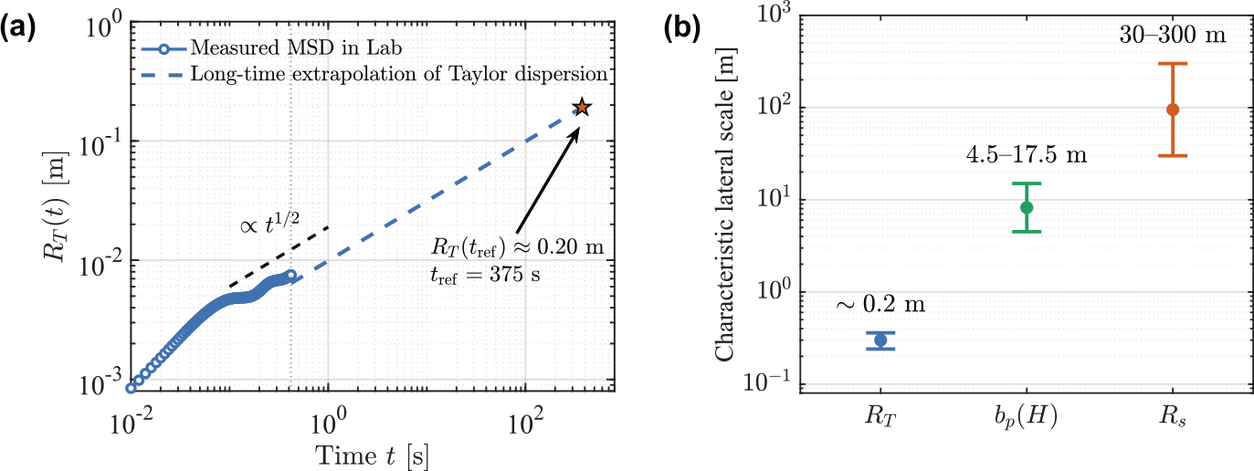
These scales are incompatible with bubble-swarm Taylor dispersion as the controlling mechanism. To estimate the Taylor dispersion scale associated with local stochastic bubble motions, we use the laboratory measurement data from Huang et al. (Reference Huang, Hessenkemper, Tan, Ni, Sommer, Bragg and Ma2025 a) (case La); see figure 2(a). The symbols show the lateral displacement scale obtained directly from the measured bubble MSD while the dashed line denotes the long-time extrapolation $R_T=(2D_bt)^{1/2}$ . Here, $D_b$ is determined independently from the measured lateral bubble-velocity fluctuations and their Lagrangian correlation time. For case La, the measured lateral bubble-velocity fluctuation is $\sigma _{u_b}=0.0835\,\mathrm{m\,s^{-1}}$ and the asymptotic lateral correlation time is $T_{L,u_b}=0.007\,\mathrm{s}$ . This gives $D_b=4.88\times 10^{-5}\,\mathrm{m^2\,s^{-1}}$ (Huang et al. Reference Huang, Hessenkemper, Tan, Ni, Sommer, Bragg and Ma2025 a). We evaluate the scale of lateral displacement of Taylor dispersion at a reference time $t=t_{\textrm {ref}}=H/W$ , with $H\simeq 75\,\mathrm{m}$ the water depth of the pipeline rupture and $W=0.20\,\mathrm{m\,s^{-1}}$ the measured mean rise velocity of bubbles in case La. This gives $t_{\textrm {ref}}\simeq 375\,\mathrm{s}$ and $R_T\simeq 0.2\,\mathrm{m}$ (figure 2 a). Because this laboratory-based reference time is much longer than the simulated Nord Stream surfacing time $t_a\simeq 27\,\mathrm{s}$ , it provides a conservative upper estimate of $R_T$ and hence a lower estimate of $\unicode{x1D6F1}$ .

Figure 2.

(a) Bubble Taylor-dispersion scale obtained from the measured horizontal MSD and its long-time extrapolation using the experimentally determined diffusivity (Huang et al. Reference Huang, Hessenkemper, Tan, Ni, Sommer, Bragg and Ma2025 a). (b) Comparison with focused-fountain and surface-spread radii reported for Nord Stream.

The same conclusion follows from an inverse estimate. If a lateral radius $R=O(10)$ – $O(100)\,\mathrm{m}$ were attributed to Taylor dispersion over the initial Nord Stream ascent time $t_a\simeq 27\,\mathrm{s}$ , the required diffusivity would be $D_{\textrm {req}}\sim R^2/2t_a=O(1){-}O(10^2)\,\mathrm{m^2\,s^{-1}}$ which is $10^4$ – $10^6$ times larger than the laboratory Taylor diffusivity. Thus, Taylor dispersion may occur locally inside the bubbly flow, but it cannot set the scale of focused-fountain or surface-patch width.

A possible objection to this comparison is that the Nord Stream release occurred in the ocean and involved much larger Reynolds numbers than the laboratory bubble swarm. However, a large Reynolds number based on the water depth, source scale or observed surface-patch scale does not by itself imply a proportionally large local Taylor diffusivity $D_b$ . It mainly indicates a large separation between the outer and viscous scales of the flow. The $D_b$ relevant here is instead controlled by local bubble velocity fluctuations and their Lagrangian decorrelation time. In simple scaling form, the diffusivity is set by local bubble motion, not by the oceanic outer scale.

The laboratory case is therefore used here only as a reference estimate for the local stochastic contribution associated with bubble spreading in a swarm. Although the water in the experiment of Huang et al. (Reference Huang, Hessenkemper, Tan, Ni, Sommer, Bragg and Ma2025 a) was initially quiescent, the bubble swarm itself generated wake-induced fluctuations and bubble–bubble interactions. The near-field Nord Stream plume was certainly far more energetic, but its energetic motions were coherent plume-scale motions: entrainment during ascent, penetration of the sea surface as a fountain, collapse of that fountain and radial surface spreading.

The focused-fountain scale is instead consistent with plume-entrainment estimate introduced in § 2.2. For $H\sim 70{-}88$ m, $b_0=O(1)\,\mathrm{m}$ (pipe size), the estimate $2b_p\sim 2(b_0+6/5\alpha _e H)$ gives $2b_p\approx 9$ –35 m, consistent with the previously reported 11–31 m fountain diameter (Dissanayake et al. Reference Dissanayake, Gros, Drews, Nielsen and Drews2023).

The larger 100–750 m surface expression requires the free surface. Once the plume reaches the interface, fountain collapse can drive a radial surface current, analogous to top-current or intrusion behaviour in plume systems (Cardoso and Cartwright Reference Cardoso and Cartwright2024; Woods Reference Woods2010). This surface current transports entrained water and gas constituents over O(100 m) scales. A simple estimate gives the same order of magnitude. Using the surface-spreading scale $R_s\sim U_s t_{\textrm {res}}$ introduced in § 2.3, and taking $U_s\sim 3\,\textrm {m}\,{\rm s}^{-1}$ from the radially spreading surface-plume model of Dissanayake et al. (Reference Dissanayake, Gros, Drews, Nielsen and Drews2023) and $t_{\textrm {res}}\sim O(10^1)$ – $O(10^2)\,\textrm {s}$ from laboratory observations of surface-bubble persistence in saline solutions (Anguelova and Huq Reference Anguelova and Huq2017), gives $R_s\sim 30$ – $300\,\textrm {m}$ (figure 2 b). 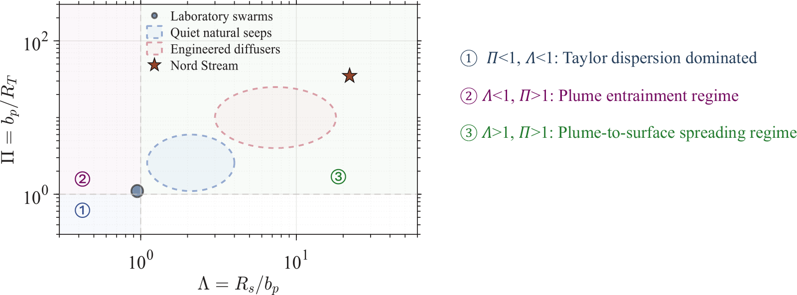Using the conservative value $R_T\simeq 0.2\,\mathrm{m}$ together with the full estimated ranges of $b_p$ and $R_s$ gives $\Pi \simeq 23$ – $88$ and $\varLambda \simeq 1.7$ – $67$ , both remaining above unity. Delayed coalescence in the brackish Baltic Sea water may help sustain the visible foam; atmospheric observation studies also note foamy seawater patches of several hundred metres that persisted for about one week (Harris et al. Reference Harris, Schwietzke, France, Velandia Salinas, Meixus Fernandez, Randles, Guanter, Irakulis-Loitxate, Calcan, Aben, Abrahamsson, Balcombe, Berchet, Biddle, Bittig, Böttcher, Bouvard, Broström, Bruch, Cassiani, Chipperfield, Ciais, Damm, Dammers, Denier van der Gon, Dogniaux, Dowd, Dupouy, Eckhardt, Evangeliou, Feng, Jia, Jiang, Kaiser-Weiss, Kamoun, Kerridge, Lampert, Lana, Li, Maasakkers, Maclean, Mamtimin, Marshall, Mauger, Mekkas, Mielke, Mohrmann, Moore, Nanni, Pätzold, Pison, Pisso, Platt, Préa, Queste, Ramonet, Rehder, Remedios, Reum, Roiger, Schmidbauer, Siddans, Sunkisala, Thompson, Varon, Ventress, Wilson and Zhang2025). The physical sequence is therefore pipe rupture $\rightarrow$ gas jet $\rightarrow$ entraining plume $\rightarrow$ surface fountain $\rightarrow$ radial spread. Bubble-scale Taylor dispersion may occur inside the flow, but it does not set the dominant width.