Introduction
The White Mountains in New Hampshire (Fig. 1) extend ~90 km north–south and 60 km east–west. Altitudes in this part of the northern Appalachian Mountains range from as low as 150 m in river valleys to 1917 m on the summit of Mount Washington (the highest peak in the northeastern United States). The most recent continental glaciation occurred when the late Wisconsinan Laurentide Ice Sheet (LIS) expanded generally southward across the state. The White Mountains were completely covered by the ice sheet during the last glacial maximum (Bierman et al., Reference Bierman, Davis, Corbett, Lifton and Finkel2015). Prior to this time, small alpine glaciers carved cirques on the flanks of Mount Washington and other peaks in the Presidential Range (Goldthwait, Reference Goldthwait1970; Davis, Reference Davis1999).
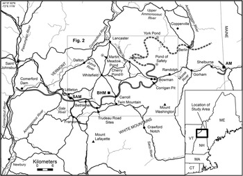
Map showing principal towns (black dots), roads (black lines), and rivers (thin gray lines) in the study area; the area covered by Figure 2; and locations of glacial readvance sites at Comerford Dam, Trudeau Road area in Bethlehem, and the Corrigan pit in Randolph, New Hampshire. Long, solid gray line indicates the southern limit of the Littleton-Bethlehem readvance and related moraines (White Mountain Moraine System) as defined by Thompson et al. (Reference Thompson, Fowler and Dorion1999). Dashed gray line shows correlation with the Berlin moraines (Fig. 2). Short gray line on the Maine–New Hampshire border marks the Androscoggin moraine cluster (AM). Open circles are pond coring sites. Black squares indicate sample locations for cosmogenic-nuclide exposure dating: Sleeping Astronomer moraine (SAM), Beech Hill moraines (BHM), and Androscoggin moraines (AM).
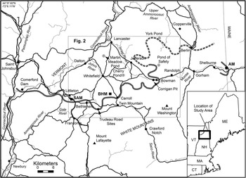
Numerous moraines were deposited by closely spaced readvances and stillstands as the LIS retreated from the study area. The moraine belt, which we refer to as the White Mountain Moraine System (WMMS), spans the entire width of northern New Hampshire. The local abundance of these deposits contrasts with the general scarcity of moraines across interior northern New England. The close association of the WMMS with a well-defined sequence of ice-dammed glacial lakes and the varve series of glacial Lake Hitchcock in the Connecticut River valley has generated renewed interest in the deglaciation and climate history of the region.
We bring together several investigative threads documenting late-glacial environments of the northern White Mountains to update work by Ridge et al. (Reference Ridge, Besonen, Brochu, Brown, Callahan, Cook, Nicholson and Toll1999) and Thompson et al. (Reference Thompson, Fowler and Dorion1999), including data from new fieldwork. Our findings are tied to advances in deglaciation chronology resulting from the work of Ridge et al. (Reference Ridge, Balco, Bayless, Beck, Carter, Dean, Voytek and Wei2012) on the North American Varve Chronology (NAVC) and cosmogenic-nuclide exposure studies by Balco et al. (Reference Balco, Briner, Finkel, Rayburn, Ridge and Schaefer2009). Our objectives are to (1) define the extent and character of the WMMS and associated glacial lakes, (2) determine the age of the moraines and thereby facilitate cosmogenic-nuclide production rate calibration, (3) propose correlations with other glacial deposits in the region, and (4) evaluate the climatic significance of the moraine system and late-glacial climate changes in the White Mountains from pond sediment cores and the varve record.
Previous work
The White Mountains region has been one of the most controversial areas in the history of New England glacial research. The existence of moraines and mode of deglaciation were debated from the mid-1800s through the 1930s (Thompson, Reference Thompson1999). Much of the early work focused on the Ammonoosuc and other river valleys in the northwestern White Mountains. These west-draining tributaries of the Connecticut River were blocked by the LIS, resulting in a succession of ice-dammed glacial lakes that stepped down and shifted location as the ice sheet receded.
Agassiz (Reference Agassiz1870) visited the White Mountains in 1847 and published the first observations on moraines in the Bethlehem area of the Ammonoosuc River valley (Thompson, Reference Thompson1999). Upham (Reference Upham1904) coined the name “Bethlehem moraine” for these deposits and found that they are chiefly composed of till. These early workers assumed the moraines were deposited by a local glacier flowing north from the Mt. Lafayette area in the nearby Franconia Range. However, Goldthwait (Reference Goldthwait1916) proved that the Bethlehem moraine was built by a southward-flowing continental ice sheet. He also named glacial Lake Ammonoosuc, which was impounded by the retreating ice margin in the Ammonoosuc valley.
Antevs (Reference Antevs1922) inferred from his Connecticut valley varve records that a glacial readvance occurred west of Littleton where the Comerford Dam is now located (Fig. 1). He suggested that this readvance might correlate with the Bethlehem moraine. Crosby (Reference Crosby1934a, Reference Crosby1934b) reached the same conclusion, supported by the two-till stratigraphy that he found during engineering studies for the dam on the New Hampshire side of the Connecticut River. Lougee (Reference Lougee1934, Reference Lougee1935) found similar evidence on the Vermont side of the river.
Flint (Reference Flint1929, Reference Flint1930) triggered a paradigm shift regarding the mode of deglaciation in New England. He argued that recession of the last ice sheet occurred by simultaneous stagnation and downwasting over the entire region. Goldthwait (Reference Goldthwait1938, p. 349) was persuaded to reverse his earlier stance and dismiss the Bethlehem moraine as simply a “zone of massive kettled outwash.” Despite rebuttals by Antevs (Reference Antevs1939) and Lougee (Reference Lougee1940), the stagnation model prevailed until the late 1900s when evidence was found that dynamic ice persisted during deglaciation of at least the eastern White Mountains (e.g., Gerath, Reference Gerath1978; Gerath et al., Reference Gerath, Fowler and Haselton1985; Thompson and Fowler, Reference Thompson and Fowler1989).
Thompson et al. (Reference Thompson, Fowler and Dorion1999) reexamined the Bethlehem moraine complex and agreed with early workers’ correlation of the moraines with the glacial readvance at the Comerford Dam site. These authors logged the stratigraphy of new stream-bluff exposures near the dam showing till units separated by thrust-faulted sand and gravel, which indicated a readvance that probably was coeval with the readvance at the dam site. They also discovered other moraine clusters east of Bethlehem, in Carroll and Randolph, which they correlated with the Bethlehem moraines. From basal radiocarbon ages of pond sediments, Thompson et al. (Reference Thompson, Fowler and Dorion1999) inferred an age of ca. 12,000 radiocarbon years (~14 cal ka BP) for the Littleton-Bethlehem (L-B) readvance, and Ridge and Toll (Reference Ridge and Toll1999) made the same inference based on a 14C calibration of varve stratigraphy in the upper Connecticut valley at Newbury, Vermont. Based on different 14C data sets, both groups of authors proposed that the readvance may have resulted from the Older Dryas (OD) cold-climate event.
Analysis of the vegetation sequence and radiocarbon dating of lake sediments in the White Mountains have been carried out by Miller and Thompson (Reference Miller and Thompson1979), Davis et al. (Reference Davis, Spear and Shane1980), Spear (Reference Spear1989), Thompson et al. (Reference Thompson, Fowler, Flanagan and Dorion1996), Miller and Spear (Reference Miller and Spear1999), Cwynar and Spear (Reference Cwynar and Spear2001), and Dorion (Reference Dorion2002). These studies provide important data for reconstructing the climate history of the White Mountains and its impact on the earliest humans who occupied the area soon after deglaciation. One of the major findings is the discovery of the Younger Dryas (YD) climate oscillation in pond sediment cores (Thompson et al., Reference Thompson, Fowler, Flanagan and Dorion1996; Cwynar and Spear, Reference Cwynar and Spear2001; Dorion, Reference Dorion2002). The YD signal occurs in cores from three of the four ponds investigated by these authors in the area of the WMMS.
Methods
We used a four-pronged approach to investigate the WMMS: geologic mapping and stratigraphy, sediment core analysis and radiocarbon dating, varve chronology, and cosmogenic-nuclide exposure dating.
Geologic mapping and stratigraphy
Thompson and Fowler carried out detailed field mapping to test earlier correlations between individual moraine clusters within the belt, and they searched for the continuation of the WMMS to the east, in the New Hampshire–Maine border region. They also located new stratigraphic exposures and test-boring data that define the depositional environment of the moraines. The mapping component of this study included examination of new high-resolution bare-earth LIDAR imagery, which has proved very effective for locating moraines and other glacial features in densely forested terrain.
The general sequence of ice-dammed glacial lakes in the region was determined by Lougee (Reference Lougee1939). We conducted further work on this topic to precisely determine locations, water levels, meltwater feeder channels, ice-contact deltas, and spillways of the stages of glacial Lake Ammonoosuc and other lakes. The association of the lakes with the moraines provides important constraints on ice-margin positions during deglaciation and enables correlation across gaps between the moraine clusters. Thompson and Svendsen (Reference Thompson and Svendsen2015) compiled a preliminary map of ice-dammed lakes throughout the northern White Mountains, and we have added further information to that part of their map which is shown here (Fig. 2).
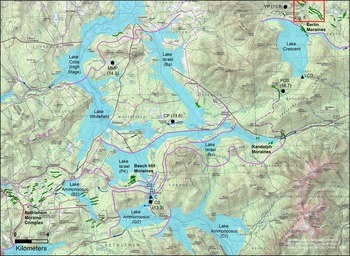
Map of northern White Mountains showing moraine clusters (green lines) deposited during the Littleton-Bethlehem readvance and recession from the readvance maximum, associated glacial lakes (blue) and lake spillways (blue arrows), recessional ice-margin positions (purple lines), and area covered by LIDAR image in Figure 5. Lake stages shown here include the following: Crawford (Cr), Gale River 2 (G2), and Bethlehem 2 (B2) stages of Lake Ammonoosuc; Lake Carroll stages C1, C2; and the Bowman (Bo), Pine Knob (PK), and Baileys (Ba) stages of Lake Israel. Black dots mark coring sites and approximate basal radiocarbon ages in cal ka BP for Pond of Safety (POS), Carroll spillway (CS), Cherry Pond (CP), Martin Meadow Pond (MMP), and York Pond (YP). Black triangles are locations of the Carroll delta (C) and Lake Crescent delta (LCD). Unlabeled glacial lakes include small parts of Lake Franconia (southwest corner of map) and two arms of Lake Hitchcock on the western border. Topographic base map contour interval is 20 m.

Sediment core analysis and radiocarbon dating
We cored late-glacial sediments beneath four ponds and one glacial lake spillway (Fig. 2). The main objective was to obtain accelerator mass spectrometry (AMS) radiocarbon ages from the deepest organic material in each core, to provide minimum-limiting ages for when the sites were deglaciated. Our second objective was to examine the lower parts of the cores for evidence of climate reversals after the pond basins were deglaciated. We expected that cooling events would be marked by an increase in minerogenic sediment deposited into a pond, resulting from factors such as increased eolian activity or paraglacial processes. These inputs would overwhelm a pond’s in situ organic productivity (gyttja deposition) and would be recorded in cores as an inorganic zone of fine sandy silt bounded above and below by olive-green organic-rich gyttja. This stratigraphic sequence was described by Stea and Mott (Reference Stea and Mott1989) from Maritime Canada. We obtained radiocarbon ages on samples from near the beginning and termination of these barren intervals to establish their age ranges. Laboratory radiocarbon ages from the core samples were calibrated using the IntCal13 calibration curve (Reimer et al., Reference Reimer, Bard, Bayliss, Beck, Blackwell, Ramsey and Buck2013).
Multiple, overlapping, 7.5 cm diameter piston cores were obtained from the pond bottoms. Prior to coring, we probed the sediment thicknesses with coring rods, beginning at the sediment-water interface and continuing downward to refusal. Buoys were set to mark the area with the thickest sediment accumulation, which typically occurs in the deepest basin of each pond. This is where we expected to recover the oldest sediment. The core barrel was driven to the point of refusal, which usually occurred on stony material interpreted as till or ice-contact sand and gravel. The cores were examined for horizontality of beds and laminae to eliminate cores that contained slumped material. Multiple cores from a pond were compared for equivalent lithologic zones and to ensure these intervals were present and continuous across the pond basin. We conducted loss-on-ignition (LOI) analysis on the cores to determine (1) the variability in organic percent of the sediment, to help determine its origin and detect a possible YD lithic zone, and (2) the percentage of carbonate, if present, to test for old carbon in the pond system that would affect radiocarbon ages. All laboratory procedures and calculations followed the conventions of Bengtsson and Enell (Reference Bengtsson and Enell1986). Sediment samples were disaggregated with gentle tap-water washing on 425 and 212 µm sieves. A Nikon SMZ-U dissecting microscope was used to identify and count macrofossil remains, which are listed in Table 1. The following guides aided in macrofossil identification: Campbell et al. (Reference Campbell, Hyland and Campbell1978), Crow and Hellquist (Reference Crow and Hellquist2000), Haines and Vining (Reference Haines and Vining1998), Harlow (Reference Harlow1959), Landers and Johnson (Reference Landers and Johnson1976), Levesque et al. (Reference Levesque, Dinel and Larouche1988), Martin and Barkley (Reference Martin and Barkley1961), Montgomery (Reference Montgomery1977), US Department of Agriculture (1948), Uva et al. (Reference Uva, Neal and Ditomaso1997), and Young and Young (Reference Young and Young1992). Final identification utilized the reference macrofossil collection at the Laboratory of Quaternary Paleoecology and Paleohydrology at the University of Maine. Select samples of sieved vegetation were reacted with 10% HCl to remove any carbonate.
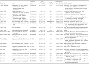
Radiocarbon and calibrated ages of samples from pond and spillway sediments at coring sites indicated in Figure 2. Calibration based on IntCal13 (Reimer et al., Reference Reimer, Bard, Bayliss, Beck, Blackwell, Ramsey and Buck2013).

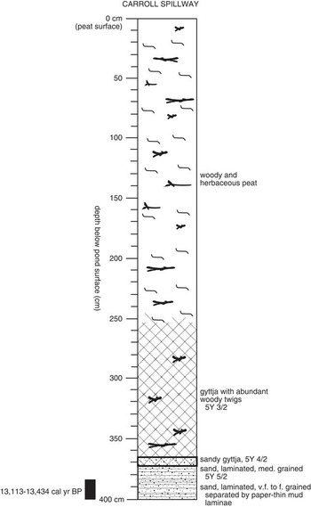
We also cored the floor of the Carroll spillway (CS, Fig. 2) with the same objectives as the pond-sediment coring. This channel carried meltwater southward from the ice margin and/or from the first stage of glacial Lake Carroll. The Carroll spillway was incised into the earlier Carroll delta (C, Fig. 2) in response to lowering of the water level in glacial Lake Ammonoosuc to the south. Very slight additional ice retreat caused the spillway to be abandoned, whereupon terrestrial plant material began to accumulate on the channel floor. We probed along transects transverse and longitudinal to the spillway axis to locate sites where the earliest organic material would have accumulated, and this material was sampled for radiocarbon dating.
Varve chronology
From 2007 to 2010, Ridge and his students along with Balco revised Ernst Antevs’ (Reference Antevs1922, Reference Antevs1928) New England Varve Chronology through the collection and measurement of subsurface cores in critical areas of the Connecticut River valley (Ridge et al., Reference Ridge, Balco, Bayless, Beck, Carter, Dean, Voytek and Wei2012). A new NAVC was formulated with a revised numbering system that is a continuous 5659 yr sequence spanning the history of deglaciation from central Connecticut up the Connecticut valley into Québec (18.2–12.5 cal ka BP). This effort resulted in the following: (1) minor corrections of Antevs’ chronology; (2) closure of the Claremont Gap that separated two major sequences in Antevs’ (Reference Antevs1922) original chronology in the Connecticut valley; (3) extension of the chronology with detailed measurement and integration of a sequence of nonglacial varves at Newbury, Vermont (Ridge and Toll, Reference Ridge and Toll1999); (4) calibration of the chronology with many new radiocarbon ages from the varves that allowed a statistical best fit with IntCal09 radiocarbon calibration data (Reimer et al., Reference Reimer, Baillie, Bard, Bayliss, Beck, Blackwell and Ramsey2009); and (5) discovery of a stadial- to subcentury-scale similarity of varve thickness records with oxygen isotope records from the Greenland Ice Sheet (Ridge et al., Reference Ridge, Balco, Bayless, Beck, Carter, Dean, Voytek and Wei2012). An update of the previous IntCal09 varve calibration (Ridge et al., Reference Ridge, Balco, Bayless, Beck, Carter, Dean, Voytek and Wei2012) using IntCal13 (Reimer et al., Reference Reimer, Bard, Bayliss, Beck, Blackwell, Ramsey and Buck2013) is presented here, and the varve/ice core correlations provide a detailed chronology of the period of the L-B readvance that is linked to climate change.
Cosmogenic-nuclide exposure dating
The moraines in the study area are densely covered with boulders, and thus their age can potentially be determined by cosmogenic-nuclide exposure dating. However, as we discuss subsequently, the moraine complex can already be dated very precisely—more precisely than would be feasible using exposure-dating methods—by its stratigraphic relationship to the NAVC. Thus, several studies that have collected cosmogenic-nuclide measurements from these moraines have aimed not at independently determining the age of the moraines, but at improving calibration of cosmogenic-nuclide production rates by comparison of exposure-age results with the moraine age inferred from the NAVC. Balco et al. (Reference Balco, Briner, Finkel, Rayburn, Ridge and Schaefer2009) used cosmogenic 10Be measurements from the Sleeping Astronomer moraine (part of the Bethlehem moraine complex discussed subsequently) and the Beech Hill moraines (Figs. 1 and 2) to show that previously available production rate calibration data yielded incorrect exposure ages for late-glacial deposits in New England. Subsequently, additional 10Be and 26Al measurements on boulders from the Beech Hill moraines were collected in the production rate calibration study described by Borchers et al. (Reference Borchers, Marrero, Balco, Caffee, Goehring, Lifton, Nishiizumi, Phillips, Schaefer and Stone2016).
To summarize, although there exist a large number of cosmogenic-nuclide measurements on boulders from moraines described here, cosmogenic-nuclide production rate estimates that we would use to compute exposure ages for these boulders are in part based on the assumption that the true age of the moraine complex is already known from correlation with the NAVC. Thus, these data do not provide an independent age for the moraines. However, they do provide a potential means of assessing the relative age of different parts of the moraine complex, which is our aim in this article. Thus, we first assume that the true exposure age of the Bethlehem and Beech Hill moraines is 13,900 cal yr BP, as inferred from correlation with the NAVC as discussed subsequently. We then use the production rate scaling scheme of Stone (Reference Stone2000) as implemented in Balco et al. (Reference Balco, Stone, Lifton and Dunai2008) to compute the reference 10Be production rate that results in the best fit between computed exposure ages for boulders on these moraines and the assumed true age, and we further assume that the 26Al/10Be production ratio is 6.75. This yields reference production rates of 3.97 atoms g-1 yr-1 and 26.77 atoms g-1 yr-1 for 10Be and 26Al, respectively, which are indistinguishable from the results of Balco et al. (Reference Balco, Briner, Finkel, Rayburn, Ridge and Schaefer2009) and Borchers et al. (Reference Borchers, Marrero, Balco, Caffee, Goehring, Lifton, Nishiizumi, Phillips, Schaefer and Stone2016). Finally, we use these reference production rates with the same scaling method to compute exposure ages for boulders from the Sleeping Astronomer and Beech Hill moraines, as well as for boulders from the Androscoggin moraine (Fig. 1) analyzed by Bromley et al. (Reference Bromley, Hall, Thompson, Kaplan, Garcia and Schaefer2015). All field and analytical data for these samples are already reported in Balco et al. (Reference Balco, Briner, Finkel, Rayburn, Ridge and Schaefer2009), Thompson et al. (2009a), Borchers et al. (Reference Borchers, Marrero, Balco, Caffee, Goehring, Lifton, Nishiizumi, Phillips, Schaefer and Stone2016), and Bromley et al. (Reference Bromley, Hall, Thompson, Kaplan, Garcia and Schaefer2015), so we have not reproduced them here. In addition, all field and analytical data for the Sleeping Astronomer and Beech Hill sites are available online via the ICE-D production rate calibration database (http://calibration.ice-d.org).
Results
WMMS
Most of the moraines in the study area are concentrated in four clusters. From west to east, these are the Bethlehem moraine complex and the Beech Hill, Randolph, and Berlin moraines (Fig. 2). The moraines in all these areas are generally similar to one another. They are composed predominantly of loose sandy till with abundant stones including many granitic boulders derived from local plutons. The moraine ridges typically are 3–30 m high and rarely as much as 50 m. Individual segments are up to 1300 m long, and most are sharp crested. The spacing between moraines varies, having depended on ice retreat rate and sediment supply. In the tight cluster of the Beech Hill moraines, it ranges from 30 m to about 200 m.
Bethlehem moraine complex
The Bethlehem moraines (Fig. 2) were deposited during ice recession from the upper Ammonoosuc valley. This is the most diffuse group of moraines in the WMMS, spanning up to 7 km of northward to northwestward ice-margin retreat. Elevations of moraine crests range from 420 m at the distal margin of the complex east of Bethlehem to 280 m at the proximal margin near the Ammonoosuc River in Littleton. A few outlying moraines of the Bethlehem complex occur in the western part of Littleton, 12 km east of the Comerford Dam readvance site. Exposures and well logs indicate the Bethlehem moraines consist chiefly of till. Thompson et al. (Reference Thompson, Fowler and Dorion1999) described a moraine cross section in Littleton village where shear structures indicated ice shove from the north. The high (30–40 m) sharp-crested moraines just southeast of Littleton were deposited in terrestrial settings at the terminus of the moraine belt, whereas some of the other moraines in the Bethlehem moraine complex formed where the ice margin stood in glacial Lake Ammonoosuc.
New information on the stratigraphy of the Bethlehem moraines has come from test borings by Sanborn, Head, & Associates (2014) at the regional landfill on Trudeau Road in Bethlehem, about 30 km east of Comerford Dam (Fig. 1). The landfill is situated on one of the most distal moraines in this part of the complex. Three of the deepest borings at the Trudeau Road site are located in the proximal part of the moraine, along an east–west line over a distance of ~340 m. The western boring (B-916D) penetrated 31 m of surficial sediments overlying bedrock. It encountered 13 m of readvance till overlying 10 m of sand, silt, and minor gravel. The latter unit in turn overlies 8 m of till. The same units occur to the east, where boring B-918D ended at ~38.5 m without reaching bedrock (3.7 m till, 29.3 m silt-sand, 5.5 m till). Still farther east, boring B-919D encountered 4.5 m of till, 42.1 m of silt-sand, 3.0 m of till/2.2 m of silt-sand.
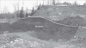
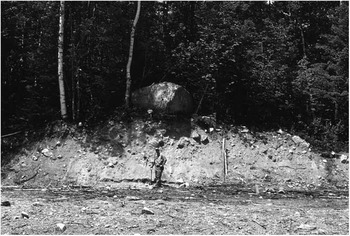
Two sand and gravel pits near the Trudeau Road landfill show readvance till overlying water-laid glacial sediments. The section in one pit exposes a moraine consisting of till overlying coarse gravel with sand lenses (Fig. 3). The other section is 1.25 km southeast of the first, in the distal flank of the same moraine on which the landfill is located. It shows silty-sandy diamict with small rounded stones overlying well-stratified glaciofluvial sand and fine gravel. The diamict is interpreted as till derived from recycling of glaciolacustrine sediments during local ice readvance. The landfill borings and nearby pit exposures collectively show that at least some of the distal Bethlehem moraines are not composed solely of till. The upper (readvance) till at all of these Bethlehem sites is thought to be equivalent in age to the upper till at Comerford Dam.
View looking southeast at longitudinal cross section of moraine ridge near Trudeau Road in Bethlehem, showing readvance till (upper pit face) overlying glacial gravel. Total exposed till thickness, including area behind upper face, is approximately 10 m. The till shows abundant shear structures and rounded stones incorporated from the gravel.

Beech Hill moraines
Thompson et al. (Reference Thompson, Fowler and Dorion1999) discovered a cluster of end moraines just north of Beech Hill in the town of Carroll (Fig. 2). These moraines are located about 7 km east of the Bethlehem moraine complex. The Beech Hill moraine cluster is at least 0.8 km wide from its distal to proximal margin, but there may be additional hummocky moraine deposits in the wooded area just to the north. Elevations of the well-defined moraines are 396–427 m. They comprise 10 till ridges that are 4–12 m high, up to 700 m long, and trend east-northeast to west-southwest. Granite boulders up to 3 m wide are abundant on the surfaces of the moraines (Fig. 4). Considering the location of the Beech Hill moraines and their relationships to local glacial-lake stages, it is reasonably certain that they correlate with the northern part of the Bethlehem moraine complex.
View looking west at cross section of one of the Beech Hill moraines. Proximal side of moraine is to the right.

Randolph moraines
Another cluster of moraines, which we correlate with the Bethlehem and Beech Hill moraines, occurs to the northeast in the Israel River valley in Randolph (Fig. 2). The Randolph moraines span about 3.4 km in the direction of downvalley ice retreat (toward the west–northwest). The largest and most distal of these moraines are located on the drainage divide at the head of the Israel valley, in the Bowman area of Randolph, where their crests reach elevations of about 540 m. The moraine crests drop to about 445 m at the proximal margin of the Randolph cluster. A major outlying moraine near the Pond of Safety coring site in the hills of northern Randolph (Fig. 2) rises to 720 m. Its location relative to the moraines at the head of the Israel valley suggests the moraines in both places were deposited by the same ice tongue and perhaps at the same time. The difference in their elevations may reflect a steep ice-surface profile near the glacier margin during the L-B readvance. These distal moraines are up to 50 m high and associated with proglacial channels that fed meltwater into neighboring river basins to the north and east.
Exposures in Randolph have recorded a glacial readvance of at least several hundred meters in the upper Israel valley. The Corrigan pit, located on the south side of Valley Road and 0.8 km east of the Jefferson–Randolph town line (Fig. 1), shows glaciolacustrine deltaic sand and gravel overlain by 6 m of stony glacial till comprising a moraine ridge. Recumbent folds and thrust faults in the upper part of the lacustrine unit indicate an ice readvance from the west, concurrent with deposition of the moraine. Overconsolidated and deformed lake sediments in other excavations near the Corrigan pit likewise have indicated a readvance into Lake Israel (Thompson et al., Reference Thompson, Fowler, Flanagan and Dorion1996, Reference Thompson, Fowler and Dorion1999).
Berlin moraines
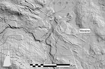
A series of moraines near the town of Berlin in the northeastern White Mountains have been mapped with the aid of LIDAR imagery (Figs. 2 and 5; Thompson et al., Reference Thompson, Boisvert, Dorion, Kirby and Pollock2009b; Thompson and Svendsen, Reference Thompson and Svendsen2015). The most clearly defined part of the moraine cluster is 3.5 km wide. Moraine crest elevations range from up to 492 m south of Jericho Lake to about 415 m in the Upper Ammonoosuc River valley. The Berlin moraines are low but very distinct till ridges that mostly trend northwest–southeast. They were deposited by ice retreating northeast from the headward part of the Upper Ammonoosuc basin. The moraines are 3–10 m high and strewn with large granitic boulders.
LIDAR image showing part of the Berlin moraines (narrow ridges extending from lower-right to upper-left part of image). Image processed by Neil Olson, New Hampshire Geological Survey. Topographic base map contour interval is 6 m in southern half of figure and 20 ft. in northern half.

Hildreth’s (Reference Hildreth2009) mapping showed a prominent moraine just west of the Pond of Safety coring site in Randolph (Fig. 2), on the divide between the Israel River and Upper Ammonoosuc River basins. As noted previously, this deposit is an outlying member of the Randolph moraines. LIDAR imagery reveals multiple channels that drained meltwater north from the Pond of Safety moraine and supplied sediment to the glacial Lake Crescent delta described subsequently. The position and elevation of this delta require that the Upper Ammonoosuc valley was dammed by the ice margin that deposited the Berlin moraines, thus showing that the Berlin moraines are coeval with the Randolph moraines and likewise part of the WMMS (Fig. 1).
Gerath (Reference Gerath1978) mapped the Copperville and Success moraines in the Berlin area. The Copperville moraine is near the proximal margin of the Berlin moraines, ~11 km northwest of the town of Berlin. This deposit consists of ice-contact outwash at the head of the Dead River valley. The Success moraine is close to the Maine border, ~5–8 km east–northeast of Berlin. The latter feature is a group of meltwater channels and ice-contact sand and gravel deposits with evidence of minor glacial readvance. The Copperville and Success deposits mark recessional ice-margin positions that probably correlate in time with the WMMS, but they are water-lain features, in contrast to the till moraines that we discuss here. Our reconnaissance fieldwork in adjacent Maine has not located an eastward continuation of the WMMS.
Glacial lake sequence
Ice-dammed lakes directly associated with the WMMS existed in the Ammonoosuc, Johns, Israel, and Upper Ammonoosuc River basins (Figs. 1 and 2). Most of these lakes had multiple stages because ice retreat opened successively lower spillways through gaps in the surrounding hills or across earlier moraines and deltas. Successive stages of each lake shifted downvalley as new spillways became available.
Lake Ammonoosuc
Glacial Lake Ammonoosuc occupied the upper part of the Ammonoosuc River basin, from Crawford Notch west to Bethlehem (Fig. 2). Thompson et al. (Reference Thompson, Fowler and Dorion1999) defined nine stages of this lake, of which three representative examples are shown in Figure 2 to illustrate the pattern of ice retreat. The earliest was the Crawford stage (CR, Fig. 2) which drained southward through Crawford Notch (Fig. 1). Five later and progressively lower stages of Lake Ammonoosuc drained southwestward into the upper Gale River valley in Franconia. Each stage can be associated with a particular spillway channel. For example, the spillway for the second Gale River stage (G2, Fig. 2), which may have been the widest and deepest stage, is a prominent abandoned channel now seen along U.S. Route 3 southwest of Twin Mountain village (Figs. 1 and 2). The log for a well (CFW 53; Flanagan, Reference Flanagan1996) near Twin Mountain shows a contact between thick glaciolacustrine clay and the underlying till at an elevation of 401 m. Comparison with the G2 spillway elevation of 445 m indicates a water depth of at least 44 m. Later spillways north of Bethlehem village drained the last three stages of Lake Ammonoosuc westward into the lower Gale River and Ammonoosuc River.
Lakes Carroll, Israel, and Whitefield
Three closely related glacial lakes developed as the ice receded northward from the Ammonoosuc valley. Lake Carroll formed north of Twin Mountain village, just south of the Beech Hill moraines. The first stage of this lake (C1, Fig. 2) was very small and briefly drained south through the 429 m channel that incises the Carroll delta. Lake Carroll then dropped to the C2 stage as it drained west along the ice margin.
At the same time that glacial Lake Carroll existed, deglaciation of the neighboring Israel valley to the east resulted in the first stage of ice-dammed Lake Israel. This stage (Bo, Fig. 2) drained east across the divide at Bowman and into the Moose River valley. Deltaic and subaqueous fan deposits were built into the Bowman stage lake. With further ice retreat, lake waters in the Israel valley may have briefly expanded west as the Pine Knob (PK) stage and drained through a 387 m col into the Ammonoosuc valley, as shown in Figure 2.
Slight additional recession led to the creation of two separate lakes: the Baileys stage of Lake Israel to the east and Lake Whitefield to the west. The Baileys stage (Ba) spilled west across a low divide at Cherry Pond in Jefferson and thence into Lake Whitefield. Lake Israel terminated when ice retreat to Lancaster caused it to merge with glacial Lake Coos in the Connecticut River valley. Lake Coos (Fig. 2) was a large drift-dammed lake just north of glacial Lake Hitchcock. During ice retreat from the study area, it extended from Dalton, New Hampshire, up the Connecticut valley to North Stratford (Thompson et al., Reference Thompson, Ridge and Springston2011). Lake Whitefield occupied the Johns River valley as the ice margin receded north from Whitefield village. This lake initially drained south into the Ammonoosuc River and with further ice recession likewise dropped and merged with Lake Coos.
Lake Crescent
Recessional ice-margin positions indicated by the Berlin moraines suggest that an ice-dammed lake existed in the Upper Ammonoosuc River valley, in the northeast part of the study area (Figs. 1 and 2) and distinct from the Ammonoosuc River basin discussed previously. The headwaters of this river occupy a mountain-rimmed basin that drains to the north and would have been blocked by the northeast-retreating ice lobe that deposited the moraines. A series of nine meltwater channels drained the basin along its eastern border. These channels are lower to the north, recording a succession of probable lake spillways that opened as the ice receded (Thompson and Svendsen, Reference Thompson and Svendsen2015). The dense forest cover and poor exposure of Pleistocene deposits in the Upper Ammonoosuc valley hindered recognition of lacustrine deposits when the area was mapped by Hildreth (Reference Hildreth2009). However, LIDAR imagery shows a delta complex at the head of the basin that was built by glacial meltwater streams flowing northward into the former lake. Elevations of terraces on the delta top correspond with some of the spillway channels mentioned previously, confirming the lowering of the lake level with time. On the basis of this evidence, we have identified an ice-dammed lake called glacial Lake Crescent after the neighboring Crescent Range (Fig. 2).
Late-glacial stratigraphy and radiocarbon dating of pond sediments
Deglaciation of pond basins
We found that the basal portion of a typical pond-sediment core from the White Mountains consists of light-gray, silty-sandy, rhythmically laminated lacustrine sediment containing sparse plant and insect remains. This bottommost unit was deposited during uncovering of the pond basin by glacial recession. We interpret the rhythmic lamination of the unit as representing deposition from sediment-laden glacial meltwater directly entering the pond’s catchment. This implies that some portion of the ice margin must have lain in the watershed when the earliest pond sediments accumulated. Therefore, the radiocarbon ages obtained from basal sediments at our pond coring sites were expected to provide close minimum limits for the time of deglaciation. Above this basal portion, we observed a transition to organic-rich sediment (gyttja, or minerogenic gyttja), interpreted to signal the cessation of glacial meltwater entering the pond’s catchment. This interpretation is identical to that of Briner et al. (Reference Briner, Stewart, Young, Philipps and Losee2010) from pond cores along the Greenland Ice Sheet’s western margin.
Results from sediment cores
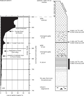
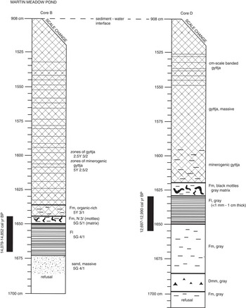
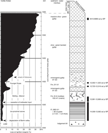
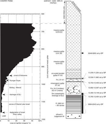
Table 1 shows the sample ages and identification of the dated material from our sediment cores; detailed core logs are provided in Figures 6–10. We cored Pond of Safety in Randolph, which is just outside the moraine belt (POS, Fig. 2; Fig. 6), because its location in the hills north of the Presidential Range was expected to provide a maximum-limiting age for the moraines to the southwest. The basal age from Pond of Safety is ~14,660 cal yr BP (12,450±60 14C yr BP; OS-7125). This age is consistent with most other basal radiocarbon ages obtained from ponds in northern New Hampshire and adjacent parts of Québec and Maine. For example, Surplus Pond—located 48 km to the northeast in a similar mountain basin—yielded an age of ~14,140 cal yr BP (12,250±55 14C yr BP; OS-7119) (Thompson et al., Reference Thompson, Fowler, Flanagan and Dorion1996, Reference Thompson, Fowler and Dorion1999). These results support the feasibility of using either bulk gyttja or macrofossils/insect parts from ponds across the region to establish an approximate deglaciation chronology.
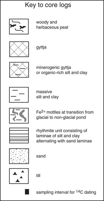
Core log for Pond of Safety, Randolph. LGM, last glacial maximum. See Fig. 6a for explanation of core-log symbols.

Key for core logs.

Core logs for Martin Meadow Pond, Lancaster. Same symbols are used as in Figure 6.

Core log for York Pond, Berlin. Same symbols are used as in Figure 6. LGM, last glacial maximum.

Core log for Cherry Pond, Jefferson. Same symbols are used as in Figure 6. GLI, glacial Lake Israel; LGM, last glacial maximum.

Core log for Carroll spillway, Carroll. Same symbols are used as in Figure 6.

We obtained a basal age of ~14,300 cal yr BP (12,360±80 14C yr BP; PL-0000491A) from the deepest core from Martin Meadow Pond (MMP, Fig. 2; Fig. 7). However, this age is older than our basal ages from coring sites associated with the WMMS, which are in more distal locations east and south of Martin Meadow Pond. The basal age from York Pond (YP, Fig. 2; Fig. 8) is ~13,800 cal yr BP (11,980±90 14C yr BP; PL-0000494A), which supports an age of ~14 cal ka BP for the Berlin moraines. Moreover, the earliest basal age from Cherry Pond, located ~11 km southeast of Martin Meadow Pond (CP, Fig. 2; Fig. 9), is likewise younger than MMP, at ~13,600 cal yr BP (11,800±80 14C yr BP; PL-0000489A). The Carroll spillway (CS, Fig. 2; Fig. 10) yielded the youngest minimum deglaciation age of all our coring sites: ~13,250 cal yr BP (11,430±80 14C yr BP; PL-0000890A). Although the spillway core penetrated typical late-glacial sandy sediment and flora (Dryas integrifolia leaves), additional coarse sands were encountered at a greater depth and thus are likely older but were not recovered with the piston corer.
We did not detect any carbonate in the pond or spillway cores. The LOI final burn at 925°C for 4 hours found no loss in sample weight, and there was no reaction with 10% HCl on sieved core samples. Bedrock underlying the study area does not contain appreciable carbonate at the coring sites or in the upglacier direction (Moench et al., Reference Moench, Boone, Bothner, Boudette, Hatch, Hussey and Marvinney1995; Lyons et al., Reference Lyons, Bothner, Moench and Thompson1997), so we are confident that the radiocarbon ages do not record old carbon from such a source. Table 1 describes the vegetation that we identified and aggregated for each radiocarbon sample. Each pond contained varying quantities and taxa of plant and insect macrofossils. The undegraded condition of the terrestrial vegetation is typical of the basal segments of pond cores from across Maine and New Hampshire. Chitinous insect parts of Coleoptera and Chironomidae were ubiquitous in the basal segments of the cores. They were likewise undegraded, suggesting quiescent, stratigraphically in situ burial. The short life span of the insects and the likely through-flow hydrogeology of the ponds would have promoted incorporation of contemporaneous atmospheric carbon from the pond water during late-glacial time. All of these physical, chemical, and biological factors enhance our confidence in the radiocarbon ages, although the two basal ages from Martin Meadow Pond and the Cherry Pond glacial-lake varves are slightly asynchronous with our regional deglaciation chronology. Taken together, the oldest basal ages from all of our coring sites except Martin Meadow Pond are consistent with deposition of the Bethlehem moraine complex ca. 14.0 cal ka BP.
The cores from Pond of Safety, York Pond, and Cherry Pond contain a barren gray minerogenic interval as shown in Figures 6, 8, and 9. Based on our limiting radiocarbon ages (Table 1), this interval records the YD cooling event that occurred between ~12.7 and 11.5 cal ka BP. Similar YD lithic zones have been found in lacustrine sediment cores from 16 widespread sites in northern Maine (Dorion, Reference Dorion1997; Borns et al., Reference Borns, Doner, Dorion, Jacobson, Kaplan, Kreutz, Lowell, Thompson and Weddle2004) and from Surplus Pond in western Maine (Thompson et al., Reference Thompson, Fowler, Flanagan and Dorion1996, Reference Thompson, Fowler and Dorion1999). Borns et al. (Reference Borns, Doner, Dorion, Jacobson, Kaplan, Kreutz, Lowell, Thompson and Weddle2004) discussed the northern Maine occurrences and their relation to YD stratigraphies in the Canadian Maritime Provinces to the east, and Dieffenbacher-Krall et al. (Reference Dieffenbacher-Krall, Borns, Nurse, Langley, Birkel, Cwynar and Doner2016) present chironomid and pollen evidence of the YD in this same part of Maine. Our findings in the White Mountains expand the YD cooling record westward across New Hampshire. Prior to our early work at Pond of Safety (Thompson et al., Reference Thompson, Fowler, Flanagan and Dorion1996), this climate event had not been documented in New England states other than Maine.
Calibrated varve chronology: age estimates, correlation, and climate
The continuous NAVC in the Connecticut valley (Ridge et al., Reference Ridge, Balco, Bayless, Beck, Carter, Dean, Voytek and Wei2012) includes the time of the L-B readvance and deposition of the WMMS to the east. The western part of the readvance is recorded near Comerford Dam (Fig. 1) where Antevs (Reference Antevs1922) originally proposed a delay in deglaciation of about 280 yr. Lougee (Reference Lougee1934, Reference Lougee1935) described an excavation at the dam showing 119 varves between till units and concluded from the number of missing varves that the readvance lasted a maximum of 151 yr. Ridge et al. (Reference Ridge, Thompson, Brochu, Brown and Fowler1996) found a nearby section that showed most of the varves present at Lougee’s site, and improved exposure of this section in later years enabled Ridge to record all 119 varves resting on till (Thompson et al., Reference Thompson, Ridge and Springston2011). These and other varve sequences in the Comerford Dam area are now correlated with the NAVC.
Revised varve calibration—IntCal13
Presented here is a revision of the NAVC calibration using IntCal13 (Reimer et al., Reference Reimer, Bard, Bayliss, Beck, Blackwell, Ramsey and Buck2013). The revised calibration follows the same procedure as the original IntCal09 version (Ridge et al., Reference Ridge, Balco, Bayless, Beck, Carter, Dean, Voytek and Wei2012) with some modifications and is as follows:
-
1. The initial trial calibration of the NAVC is based on all 54 radiocarbon ages for which there are varve year versus 14C year data in the Connecticut valley (for a list, see Ridge et al., Reference Ridge, Balco, Bayless, Beck, Carter, Dean, Voytek and Wei2012).
-
2. An assumption is made that varve years are the same as calibrated years with the only difference being their numerical starting points. Calibration of the NAVC requires finding the calibrated age of the “0” varve of the NAVC, or what is called the offset of the varve count versus calibrated years.
-
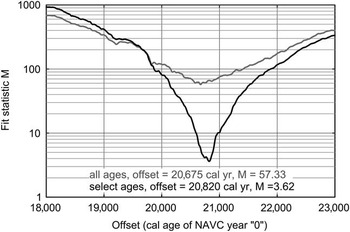
3. The best fit of the varve year versus 14C year data set with IntCal13 (calibrated year vs. 14C year data set) is determined by assuming different trial offset values (every 5 yr from 18,000–23,000 cal yr BP). The similarity of the two data sets is tested at each trial offset using a mean square of weighted deviations (M) calculation for actual 14C ages versus the expected 14C ages of IntCal13 at each trial offset (Fig. 11). The best fit has the lowest M value.
North American Varve Chronology (NAVC) calibration statistics. Plot of M, mean square of weighted deviations between measured radiocarbon ages and corresponding radiocarbon ages predicted by a chosen offset value for IntCal13, for trial offsets (every 5 yr) from 18,000 to 23,000 cal yr BP. Shown here are results for (1) all the radiocarbon ages (gray) and (2) after removing 22 radiocarbon ages (selected ages, black) that either had precision values >±200 yr or a difference of >400 yr from a calibration using all 54 ages. Calibration routine and the selection of data for the final calibration are explained in the text.

For this study, calibration was done iteratively, first using all available 14C ages. Calibration was then repeated after removing 14C ages with either poor laboratory precisions (±>200 yr) or poor fit (by >400 yr) to the initial IntCal13 calibration line derived from all the 14C ages. Poor precision values are mostly from conventional (beta counting) ages and AMS ages with very small sample masses. The 14C ages that stray from this calibration are mostly younger than the predicted 14C ages of IntCal13, which is likely the result of partial decay and imperfect preservation of plant macrofossils submitted for radiocarbon dating that likely bias the data to younger ages. Further analysis using just selected ages was repeated to include any 14C ages that were initially removed but had acceptable precisions and a <400 yr difference with the last selected age analysis. Also, ages that had a >400 yr residual with this analysis were removed. This process was repeated until the data set of selected ages had only ages different from the best fit by <400 yr (Figs. 11 and 12).
Calibration of the North American Varve Chronology (NAVC) using 32 selected radiocarbon ages (black data points; for list, see Ridge et al. Reference Ridge, Balco, Bayless, Beck, Carter, Dean, Voytek and Wei2012) and the IntCal13 data set (Reimer et al., Reference Reimer, Bard, Bayliss, Beck, Blackwell, Ramsey and Buck2013). Ages are plotted with 1-σ laboratory uncertainties as error bars. Using the selected 14C ages gives a best-fit (lowest mean square of weighted deviations; Fig. 11) offset of 20,820 cal yr BP between IntCal13 calibrated years and NAVC years, which is also the calibrated age of the NAVC “0” varve.

Results of this iterative statistical analysis indicate that the best-fit calibration is either (1) calibrated year age [cal yr BP]=20,675 yr – NAVC yr, when using all 54 14C ages, or (2) calibrated year age [cal yr BP]=20,820 yr – NAVC yr, when using 32 selected 14C ages after the iterative analysis that excluded ages with laboratory precisions of ±>200 yr or that had a difference from the calibration line of >400 yr. Ages in years before AD 2000 (b2k) are calculated by adding 50 yr to the calibrated ages in the previous equations.
Age of the L-B readvance and ice recession rates
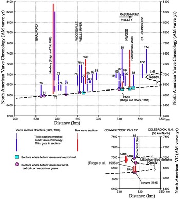
The rate of deglaciation leading up to the L-B readvance can be determined from localities where basal varves rest on till or where thick ice-proximal varves that were deposited within a decade or two of deglaciation are recorded at the bottoms of varve sections (Fig. 13). Prior to the readvance, ice receded northward from the Claremont, New Hampshire, area at a rate of ~300 m/yr along the axis of the Connecticut valley (Ridge et al., Reference Ridge, Balco, Bayless, Beck, Carter, Dean, Voytek and Wei2012).
(color online) Time-distance plot of the time spans of all measured varve sections in the upper Connecticut and Passumpsic valleys of northern Vermont and New Hampshire (updated from Ridge, Reference Ridge2004). The distance axis on all plots is measured along the axis of the Connecticut valley from an arbitrary position at Glastonbury, Connecticut. The time axes are North American Varve Chronology years. The dashed line connecting basal and ice-proximal varve localities represents the age of deglaciation.

Varve sequences in the Connecticut valley matched to the NAVC occur both above and beneath the clayey till deposited at the western limit of the L-B readvance in the Connecticut valley on the Vermont side of the Comerford Dam (Fig. 13; Ridge et al., Reference Ridge, Thompson, Brochu, Brown and Fowler1996; Ridge, Reference Ridge2003, Reference Ridge2004). NAVC varve 6836 is the youngest varve overlain by the readvance till, and NAVC varve 6987 is the oldest varve lying on top of the till. Thus, the till, and therefore the readvance it represents, had to form between varve yr 6836 and 6987, an approximately 150 yr span. There are an unknown number of varves that were subglacially eroded at this location by the readvance. The NAVC calibration brackets the age of the readvance maximum at the Comerford Dam site as NAVC yr 6836–6987 or 13,833–13,984 cal yr BP with the understanding that the calibration of the varves has an uncertainty of at least a century. This age estimate indicates an OD age as defined in ice core records (Greenland stadial 1d [GI-1d]; Lowe et al., Reference Lowe, Rasmussen, Björck, Hoek, Steffensen, Walker and Yu2008). This age also closely matches the age of wood overrun by the Middlesex readvance farther west in Vermont (13,561–13,827 cal yr BP 2σ range; 11,900±50 14C yr BP [GX-26457-AMS]; Larsen, Reference Larsen2001). The readvance at the Comerford Dam is likely the equivalent of a readvance and end moraine described by Antevs (Reference Antevs1928) a few kilometers away at St. Johnsbury, Vermont, in the Passumpsic valley. Other correlations in Vermont proposed by recent workers are discussed subsequently.
Following the L-B readvance, recession of the ice sheet in the northern Connecticut valley was rapid. Recession was at a rate of at least 200 m/yr along the axis of the valley (Ridge et al., Reference Ridge, Balco, Bayless, Beck, Carter, Dean, Voytek and Wei2012). This chronology is based on calibrated 14C ages of plant macrofossils in varved lake beds at Columbia Bridge, Vermont (Miller and Thompson, Reference Miller and Thompson1979), which indicate that ice had receded to the Vermont-Québec border by at least 13.4 cal ka BP. Rapid ice recession fits the regional picture of deglaciation developed in Québec and the Champlain valley. Parent and Occhietti (Reference Parent and Occhietti1988, Reference Parent and Occhietti1999) used shell ages from near the upper marine limit in southeastern Québec to infer deglaciation and marine transgression in the St. Lawrence Lowland north of New Hampshire at ca. 14.0 cal ka BP. However, Occhietti and Richard (Reference Occhietti and Richard2003) and Richard and Occhietti (Reference Richard and Occhietti2005) evaluated the marine reservoir effect on shell ages and proposed that the LIS receded from the White Mountains to southeastern Québec somewhat later, about 14 to 13 cal ka BP.
Character of climate during the L-B readvance interval
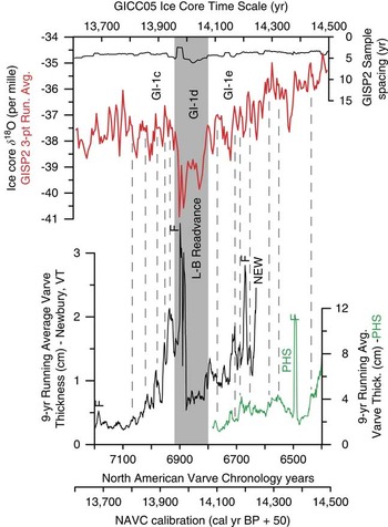
Thickness records of glacial varves from the NAVC represent a record of meltwater production and therefore a proxy of climate during deglaciation. Variations in varve thickness are mostly controlled by summer temperature and give the precise beginning and ending points as well as structure of the cooling event that caused the L-B readvance. Using the IntCal13 calibration of the NAVC, the varve records can be compared to independently calibrated oxygen isotope records from the Greenland Ice Sheet. The records show an alignment of similar patterns at not only a stadial but also a subcentury scale from ~15 to 13.5 ka b2k (Ridge et al., Reference Ridge, Balco, Bayless, Beck, Carter, Dean, Voytek and Wei2012). Shown in Figure 14 is a portion of this comparison for NAVC varve yr 6400–7200 that spans the time of the L-B readvance. The oxygen isotope record used for this analysis is from the Greenland Ice Sheet Project 2 (GISP2) ice core (Stuiver et al., Reference Stuiver, Grootes and Braziunas1995; Stuiver and Grootes, Reference Stuiver and Grootes2000 [nonaveraged continuous original measurements available at http://depts.washington.edu/qil/]) calibrated to the Greenland Ice Core Chronology 2005 (GICC05) time scale (Andersen et al., Reference Andersen, Svensson, Johnsen, Rasmussen, Bigler, Röthlisberger and Ruth2006; Rasmussen et al., Reference Rasmussen, Andersen, Svensson, Steffensen, Vinther, Clausen and Siggaard-Andersen2006, Reference Rasmussen, Seierstad, Andersen, Bigler, Dahl-Jensen and Johnsen2008; Svensson et al., Reference Svensson, Anderson, Bigler, Clausen, Dahl-Jensen, Davies and Johnsen2006) because it has the highest resolution for comparison to the varve records. The alignment of the two records occurs with an offset of their independent time scales of just +5 yr (ice core record older), which is well within the uncertainty of both time scales. Uncertainty in the ice core time scale is +180 to +156 yr for layer counts in this interval (14.5–13.6 ka b2k; Rasmussen et al., Reference Rasmussen, Andersen, Svensson, Steffensen, Vinther, Clausen and Siggaard-Andersen2006), which is tabulated as a positive departure from a conservative layer total. The varve calibration has an uncertainty of at least a century (see Fig. 12) and is likely in error by being too young as was discussed previously. If the alignment of events on both records represents an exact time correlation, and the true age of the varve chronology is older than shown by about a century, the ice core layer counts may be too few by about 100 yr as well.
(color online) A comparison of North American Varve Chronology (NAVC) varve records (bottom) and the GISP2 ice core oxygen isotope record from the Greenland Ice Sheet (top) from 14,500 to 13,600 yr before AD 2000 (b2k). Connecticut valley NAVC records (9 yr running averages, NAVC varves 6400–7200) are from Newbury, Vermont (NEW; Ridge and Toll, Reference Ridge and Toll1999), and North Charlestown, New Hampshire (PHS; Ridge et al., Reference Ridge, Balco, Bayless, Beck, Carter, Dean, Voytek and Wei2012). The calibrated time scale applied to the NAVC (Fig. 12) is here converted to years b2k to match the standard for ice cores. The GISP2 oxygen isotope record is calibrated to the Greenland Ice Core Chronology 2005 (GICC05) ice core time scale (Andersen et al., Reference Andersen, Svensson, Johnsen, Rasmussen, Bigler, Röthlisberger and Ruth2006; Rasmussen et al., Reference Rasmussen, Andersen, Svensson, Steffensen, Vinther, Clausen and Siggaard-Andersen2006, Reference Rasmussen, Seierstad, Andersen, Bigler, Dahl-Jensen and Johnsen2008; Svensson et al., Reference Svensson, Anderson, Bigler, Clausen, Dahl-Jensen, Davies and Johnsen2006) and is the continuous nonaveraged original measurements (3-point running average; Stuiver et al., Reference Stuiver, Grootes and Braziunas1995; Stuiver and Grootes, Reference Stuiver and Grootes2000) with sample spacing in GICC05 years. Varve and GISP2 data files used here are available in the supplementary data for Ridge et al. (Reference Ridge, Balco, Bayless, Beck, Carter, Dean, Voytek and Wei2012). With the proposed exact alignment of subcentury-scale and stadial-scale events in the two records, the independent time scales of the ice core and varve plots are different by only +5 yr (ice core age minus varve age) as discussed in the text. Prominent spikes in varve thickness because of nonclimatic events (marked with the letter F) are floods produced by the release of local ice-marginal lakes and lake-level changes that cannot be correlated to the Greenland record. The dark gray swath shows the period of the Littleton-Bethlehem (L-B) readvance and Greenland stadial 1d (GI-1d; Lowe et al., Reference Lowe, Rasmussen, Björck, Hoek, Steffensen, Walker and Yu2008). Thin gray tie lines indicate the coupling of subcentury warming events between the varve and ice core record (intervening cold events also match).

Alignment of features on the ice core and varve records, a characteristic that extends back to at least 15 ka b2k and through at least some earlier intervals back to 18.2 ka b2k at stadial to subcentury scales (Ridge et al., Reference Ridge, Balco, Bayless, Beck, Carter, Dean, Voytek and Wei2012), suggests that events on both records are synchronous. Some features of the varve records, such as flood events produced by the catastrophic release of water from tributary lakes impounded at the receding ice front (spikes in varve thickness marked with the letter F in Fig. 14), appear on the varve record but do not and should not have corresponding peaks on the aligned ice core record. It cannot be proved that the two records are showing synchronous features, but one of two hypotheses appears to be true: (1) the two records have similar features that are consistently offset by the same amount, or (2) the two records are synchronous. The second hypothesis seems more reasonable given the similarity of features on both records at a variety of scales.
Correlation of the Connecticut valley with the WMMS
Correlation of the maximum extent of the L-B readvance at the Comerford Dam with moraine complexes further east looks attractive from the close geographic proximity and apparent alignment of these features, but the detail with which we are now examining this system forces us to use some caution. We do not know which morainal ridge within the moraine complexes to the east correlates to the ice-maximum position at the Comerford Dam that is documented above. It may be that the most southerly of the moraine ridges in the complexes to the east correlate to the maximum extent of ice at the Comerford Dam. Alternatively, it is also possible that some of the moraine ridges represent recessional pulses or very brief stillstands that occurred just prior to the L-B readvance interval and GI-1d shown in Figure 14. There appear to be cooling events on the ice core record (most noteworthy at 14,140 and 14,090 yr b2k) that match periods of decreased varve thickness (at NAVC varves 6715 and 6765) in the century leading up to the L-B readvance/GI-1d interval (Fig. 14). At this point, we do not know what cooling threshold is required to halt ice recession and cause either stillstands or readvances. It seems possible that some of the more distal morainal ridges in the eastern moraine complexes represent oscillations that occurred during the last 200 yr of overall GI-1e cooling leading up to the sharply defined L-B/GI-1d event. If the cooling threshold necessary to generate moraines was passed prior to the time of the L-B/GI-1d interval (Fig. 14), then moraine deposition in the complexes to the east may span 200 yr (14.15–13.95 ka b2k), and some moraines could have an age that predates the ice maximum at the Comerford Dam by as much as 150 yr. Currently, it is impossible to resolve the ages of morainal ridges in the WMMS at a scale sufficient to solve this problem.
Cosmogenic-nuclide exposure ages
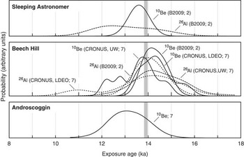
Figure 15 shows summary distributions of 10Be and 26Al exposure ages from the Sleeping Astronomer moraine near Littleton in the Bethlehem complex, the Beech Hill moraines, and the Androscoggin moraines on the Maine border (Fig. 1). Measurements on samples from the Beech Hill moraines that were made at different times and in different laboratories show small systematic offsets (Thompson et al., Reference Thompson, Balco, Dorion and Fowler2009a; Borchers et al., Reference Borchers, Marrero, Balco, Caffee, Goehring, Lifton, Nishiizumi, Phillips, Schaefer and Stone2016), so we have not averaged them. As is evident from Figure 15, both the precision of individual exposure-age measurements (~200–800 yr, excluding production rate uncertainties) and the standard deviation of exposure ages for each moraine (500–800 yr) are much larger than the length of time available for moraine formation inferred from the varve chronology (150 yr). Although mean ages for the Androscoggin and Sleeping Astronomer moraines are 800 and 600 yr, respectively, younger than the mean age of Beech Hill moraine boulders, these differences are similar to the standard deviation of ages from the individual moraines. Thus, the exposure age data are consistent with both hypotheses that (1) all three of these moraine clusters were emplaced at the same time, or (2) emplacement of the Androscoggin moraines and WMMS spanned 200 yr or more. The distal location of the Androscoggin moraines relative to the WMMS (Fig. 1) supports the latter option.
Summary normal kernel density estimates for sets of 10Be and 26Al exposure ages from the Sleeping Astronomer, Beech Hill, and Androscoggin moraines, calculated as described in the text. The vertical gray band shows the duration of the Littleton-Bethlehem readvance inferred from the North American Varve Chronology. For the Sleeping Astronomer and Beech Hill sites, sets of samples that were collected at different times and/or analyzed in different laboratories are shown separately: those labeled “B2009” were collected and analyzed by Balco et al. (Reference Balco, Briner, Finkel, Rayburn, Ridge and Schaefer2009); those labeled “CRONUS-UW” were collected as part of the “CRONUS-Earth” calibration exercise and analyzed at the University of Washington; and those labeled “CRONUS-LDEO” are aliquots of the same samples that were instead analyzed at the Lamont-Doherty Earth Observatory. Numbers in labels show number of samples in each data set; although the number of samples in each data set varies, all the probability density estimates in each panel have been normalized to have the same total area.

Discussion
The WMMS was deposited at the margin of the LIS when its steady northward recession was interrupted by the L-B readvance. We have traced this moraine belt across the full width of northern New Hampshire. It is a distinctive feature of the glacial landscape in New England, where moraines are otherwise rare and widely scattered inland from the limit of late glacial marine submergence. Field relationships between the WMMS and associated ice-dammed glacial lakes and meltwater drainage sequences indicate either that the moraine clusters formed during the same interval of time or that their ages at least overlap along the strike of the moraine system.
Our basal radiocarbon ages from pond sediment cores initially suggested deposition of the WMMS between about 14.7 and 13.3 cal ka BP, and hence the possibility that the L-B readvance occurred during and as a consequence of the OD cooling event (Thompson, Reference Thompson1998; Thompson et al., Reference Thompson, Fowler and Dorion1999). However, these are minimum-limiting ages, and they are not entirely consistent with the moraine sequence. The dated varve series in the Comerford Dam area, which is incorporated within the NAVC, yielded more precise results. It contains interbedded glacial readvance deposits indicating that the L-B readvance at the Comerford Dam reached its maximum at 13,984–13,833 cal ka BP. This age corresponds to the OD event in Europe, suggesting that OD cooling triggered deposition of the moraine belt and the climate shift evident in the varve sequence. The connection is strengthened by the exact correspondence of climate events recorded in Greenland ice cores and in the NAVC varve record that we have described here. Thus, our initial working hypothesis was supported by these relationships.
There seems to be general agreement that in ice core records stadial events with more negative oxygen isotope values represent cool intervals (Stuiver et al., Reference Stuiver, Grootes and Braziunas1995; Stuiver and Grootes, Reference Stuiver and Grootes2000; Rasmussen et al., Reference Rasmussen, Andersen, Svensson, Steffensen, Vinther, Clausen and Siggaard-Andersen2006; Lowe et al., Reference Lowe, Rasmussen, Björck, Hoek, Steffensen, Walker and Yu2008). There is also an indication that these variations may be driven more by winter than summer temperature changes (Denton et al., Reference Denton, Alley, Comer and Broecker2005; Kelly et al., Reference Kelly, Lowell, Hall, Schaefer, Finkel, Goehring, Alley and Denton2008). Current information does not imply that summer temperatures or length in Greenland or the adjacent North Atlantic region did not change. The correspondence of decreases in varve thickness, driven by decreases in summer melting, with more negative oxygen isotope values shows that there was a significant change in summer temperature or length at the margin of the southeastern LIS during cool Greenland stadial events. As pointed out by Ridge et al. (Reference Ridge, Balco, Bayless, Beck, Carter, Dean, Voytek and Wei2012), the matching of varve and Greenland Ice Sheet oxygen isotope records implies the following: (1) a correlation of lower Greenland winter temperature and decreased LIS summer ablation, perhaps because cooler Greenland winters correspond to longer winters and shorter melt seasons in the North Atlantic region; or (2) small summer temperature drops coincident with large drops in winter temperature occurred in both Greenland and at the LIS margin, but summer temperature decreased enough to generate significant decreases in meltwater and varve thickness; or (3) summer temperature drops in Greenland may have been muted as compared with summer temperature drops indicated by losses in varve thickness at the southeastern LIS margin. We do not know which of these scenarios occurred, but we do know that stadial cooling events in Greenland, regardless of makeup, correspond to periods of lower melting and meltwater production (thinner varves) at the margin of the LIS. The two records seem to be synchronous.
The alignment of the varve and ice core records suggests similar control of both records by climate across the North Atlantic region (Fig. 14). The L-B readvance interval was apparently caused by a cooling event that triggered a sharp drop in meltwater production and varve thickness at NAVC varve yr 6809. A matching sharp drop in temperature is depicted in the aligned ice core record. Varve thickness remained low until interrupted by flood events, and temperature remained low in Greenland. After the flood events, varves were relatively thin until the end of the L-B readvance interval when meltwater production and varve thickness suddenly increased at NAVC varve yr 6922. This increase in varve thickness is matched by a sharp rise in temperature on the ice core record. According to varve counts, the whole interval of low meltwater production (relatively thin varves) and low temperature depicted in the aligned ice record lasted no more than 113 yr or from 14,021 to 13,898 cal yr BP (NAVC yr 6809–6922), remembering that this age estimate has an uncertainty of at least a century. The cooling event that seems to be at the heart of the L-B readvance maximum in New England is matched by cooling during GI-1d (Rasmussen et al., Reference Rasmussen, Andersen, Svensson, Steffensen, Vinther, Clausen and Siggaard-Andersen2006; Lowe et al., Reference Lowe, Rasmussen, Björck, Hoek, Steffensen, Walker and Yu2008). The abruptness of the start and end of these apparently correlative events can be seen on both records, but the varve record shows these changes with annual resolution. The L-B interval started and ended in spans of a few years.
Numerous studies have identified brief climate reversals in Europe that dated to ca. 14.0 cal ka BP and likely record OD cooling. A few additional examples have been reported from eastern Canada. We examined these studies for possible analogs to the WMMS. The OD cold interval was regarded formerly as a chronozone that began ca. 14.0 cal ka BP and lasted about 200 yr (Mangerud et al., Reference Mangerud, Andersen, Berglund and Donner1974; Donner, Reference Donner1995). However, the chronologic boundaries of this and other classic subdivisions of late-glacial time in Scandinavia later proved to vary between different areas of Europe or could not be dated with accuracy sufficient to show that certain apparently matching climate events were synchronous. It became difficult to specify the age range of the OD from pollen records and other stratigraphic data, and in some areas, this event was not sufficiently distinct to be regarded as a separate chronozone (Wohlfarth, Reference Wohlfarth1996). The oxygen isotope record from the North Greenland Ice Core Project (NGRIP) and other Greenland ice cores brought the OD into sharper focus as part of the GICC05 time scale, recording this cooling event (GI-1d) between 14,075 and 13,954 yr b2k (Lowe et al., Reference Lowe, Rasmussen, Björck, Hoek, Steffensen, Walker and Yu2008). Thus, the OD event sensu stricto—as recorded in the ice cores—lasted only about 120 yr and was even shorter than proposed by workers in Europe.
Much of the stratigraphic evidence for the OD in Europe comes from dated moraines and till sheets formed during ice-margin stillstands or readvances. Olsen (Reference Olsen2002) noted that records of climate deterioration ca. 12.2–12.0 14C ka BP (14.1–13.8 cal ka BP) are widespread in Norway, including moraines and pollen records. He cited many examples, including OD glacial advances of at least 15 km and 10 km in northern Norway. Mangerud et al. (Reference Mangerud, Gyllencreutz, Lohne and Svendsen2011) reported the Skarpnes moraines dating to ca. 14 cal ka BP in the northern part of the country and the Tjøme-Hvaler moraine of the same age in the south. The latter moraine was correlated with the Trollhättan moraine in coastal southern Sweden (Lundqvist and Wohlfarth, Reference Lundqvist and Wohlfarth2001). Mangerud et al. (Reference Mangerud, AArseth, Hughes, Lohne, Skår, Sønstegaard and Svendsen2016) proposed an OD readvance of the Hardangerfjorden lobe of the Scandinavian Ice Sheet in southwestern Norway, based on shell-bearing till deposited at ~14 cal ka BP. Alpine glacial moraines of OD age have also been reported in Europe (e.g., by van Husen [Reference van Husen2011] in the eastern Alps of Austria).
Mean 10Be exposure ages obtained by Ballantyne et al. (Reference Ballantyne, Schnabel and Xu2009) from boulders on moraines deposited by the Wester Ross readvance in northwest Scotland ranged from 14.0±1.7 to 13.5±1.2 ka, depending on scaling method and surface erosion rates. These authors concluded that the moraines most likely formed in response to rapid but brief OD cooling. Brooks and Birks (Reference Brooks and Birks2000) determined from chironomid assemblages in western Europe that mean July temperatures in southeast Scotland dropped from 12.7°C to 7.8°C during OD time (ca. 14.1–13.9cal ka BP). Lang et al. (Reference Lang, Brooks, Bedford, Jones, Birks and Marshall2010) obtained similar results for chironomid assemblages from lake sediments in northwest England. The latter study revealed four cooling events during GI-1, with the greatest cooling amplitude during GI-1d (OD).
Van Raden et al. (Reference van Raden, Colombaroli, Gilli, Schwander, Bernasconi, van Leeuwen, Leuenberger and Eicher2013) obtained a high-precision record of late-glacial climate oscillations from δ18O analysis of marl deposited in Lake Gerzensee, Switzerland. Their data closely match the NGRIP δ18O record and were correlated with the GICC05 ice-core time scale. This study clearly identified the Aegelsee Oscillation (OD cooling) as having occurred over a 136 yr time span (14,044–13,908 cal yr BP). The duration of this event is similar to the 151 yr we obtained from the varve record of the L-B readvance at the Comerford Dam site.
The effects of OD cooling nearer to our study area remain poorly understood. Yu and Eicher (Reference Yu and Eicher2001) noted evidence of both OD and YD cooling in the oxygen isotope record of carbonates in cores from Crawford Lake in southern Ontario. These authors attributed their findings to atmospheric transmission of climate signals from the North Atlantic. Stea et al. (Reference Stea, Seaman, Pronk, Parkhill, Allard and Utting2011) described a readvance of the Appalachian Glacier Complex (Maritime Canada) that occurred in northern Nova Scotia ca. 13.8 cal ka BP, called the Shulie Lake Phase, which they correlated with the OD cooling in Europe. The Gilbert Lake moraine (Stea et al., Reference Stea, Seaman, Pronk, Parkhill, Allard and Utting2011) was deposited during the Shulie Lake readvance.
The previous studies include geologic records of OD cooling like those we have found in the White Mountains. The most pertinent similarities are that (1) parts of both the Fennoscandian Ice Sheet and LIS experienced stillstands or readvances resulting in moraine deposition at this time, accompanied by climatic cooling in adjacent areas; (2) ice-sheet response in some areas was very rapid and vigorous during the OD; and (3) the timing and duration of OD signals at some localities in western Europe and northeastern North America vary slightly from the GI-1d ice core record, probably because of local conditions affecting climate and ice-sheet dynamics, but in all cases the event was short lived.
Although the Lake Hitchcock varve record indicates a good match between the L-B readvance and climate events in the Greenland ice-core chronology (Ridge et al., Reference Ridge, Balco, Bayless, Beck, Carter, Dean, Voytek and Wei2012; this study), there is the question of whether the WMMS could have formed during the brief span of the OD. This is a complex question because the moraine clusters deposited during the L-B readvance vary in number, size, and spacing of moraines, as well as the widths of the clusters from their distal to proximal margins. The time span during which each cluster formed includes the intervals of ice-margin recession between moraines, plus the time occupied by pauses and minor readvances when the moraines were deposited.
The Comerford Dam exposures provide the best record of the duration of at least the western part of the L-B readvance. The varve sections described by Antevs (Reference Antevs1922), Lougee (Reference Lougee1934, Reference Lougee1935), and Ridge et al. (Reference Ridge, Thompson, Brochu, Brown and Fowler1996) indicate a single local readvance within a span of ~150 yr and now known to have coincided with OD cooling. Several pit exposures and borings in the Bethlehem and Randolph parts of the WMMS show readvance of at least a few hundred meters as described previously, but this stratigraphic evidence of readvance has been found only at or near the distal limit of the moraine system. This observation suggests that the main phase of the L-B readvance deposited the earliest part of the WMMS, which may have formed during the same 150 yr interval as the readvance till at Comerford Dam. Readvance to the southern limit of the moraine belt was followed by several kilometers of ice-margin retreat punctuated by stillstands during which recessional moraines were deposited. Some of the latter moraines are quite large, but no evidence has been found that they indicate significant readvances. As noted previously, moraines in the eastern part of the belt may have started to form during the GI-1e cooling just before the OD. This could have allowed up to about 300 yr for deposition of the entire WMMS, which we infer would have been ample time to account for their formation.
The L-B readvance may have extended westward into Vermont and correlates with the Middlesex readvance, based on Larsen’s (Reference Larsen2001) slightly younger age of ca. 13.8–13.6 cal ka BP for the latter event. No other corresponding ages have been obtained in the 55 km gap between Middlesex and Comerford Dam, but Hermanson and Dunn (Reference Hermanson and Dunn2013) found readvance deposits at East Barre, Vermont (40 km southwest of Comerford Dam), and proposed that they resulted from OD ice activity correlative with the Middlesex readvance. Wright (Reference Wright2015) reported till overlying deformed glaciolacustrine sediments at multiple sites in the upper Winooski River basin in Vermont, indicating a readvance zone extending from West Bolton southeast to the East Barre area. The distribution of these sections led Wright to propose that the ice margin may have readvanced as much as 55 km during cooling event GI-1d ca. 14.0 cal ka BP. It seems unlikely to us that such a major readvance could have occurred in response to this brief climate episode, unless it either started during the pre-OD cooling trend and/or progressed very rapidly in deep, clay-floored glacial lakes of the Winooski basin.
In a synthesis of Maine radiocarbon ages for the MOCA project (Meltwater Routing and Ocean-Cryosphere-Atmosphere-Response project, initiated through INQUA), Thompson et al. (Thompson, W.B., Weddle, T.K., Borns, H.W., Jr., unpublished report, 2013) proposed that the 12.0 14C ka BP deglaciation isochron (13.8 cal ka BP) crosses northern Maine in the vicinity of Mount Katahdin. These authors noted that no definite OD moraines had been identified in Maine but suggested a possible OD age for the Basin Ponds and Abol moraines on the flanks of Katahdin. However, recent work by Davis et al. (Reference Davis, Bierman, Corbett and Finkel2015) includes 10Be exposure ages from the Basin Ponds moraine indicating that it predates the OD by about 2300 yr. The latter authors suggest correlation of this moraine with the Oldest Dryas cooling.
Conclusions
Our study has documented the WMMS spanning northern New Hampshire. The western part of the system—the Bethlehem moraine complex—has been recognized since the 1800s, but the Beech Hill, Randolph, and Berlin moraines were discovered during our field investigations of recent years. These moraine clusters formed at the margin of the LIS during the late-glacial L-B readvance and oscillatory retreat from the readvance limit. Many of the moraines are associated with shallow ice-dammed glacial lakes, and stratigraphic sections near the distal margin of the moraine system indicate local overriding and deformation of lake sediments. Our mapping of lake stages, spillways, and deltas has defined and correlated ice-margin positions between the moraine clusters.
The revised calibration of the NAVC presented here shows a close match between the timing of Greenland climate oscillations and the varve record of deglaciation and glacial events including the L-B readvance. Thus, we attribute this readvance to the GI-1d cold-climate episode in the GICC05 time scale based on Greenland ice cores. The age of the GI-1d interval indicated by the Lake Hitchcock varve series is 14,021–13,898 cal yr BP, but given the uncertainties of radiocarbon ages used to calibrate the varves, and the uncertainties of the ice core time scale, the readvance may be a century older.
Our research on the WMMS provides the first described and dated record of the OD event in the northeastern United States. The robust moraine clusters of the WMMS suggest a rapid response of the LIS to OD cooling in the White Mountains. We infer that the moraine system formed as a consequence of general climate deterioration in the North Atlantic region and probably was initiated by the GI-1e cooling immediately before the OD. The rapidity of the ice sheet’s response to this climate change was more likely because of a decrease in ablation rates rather than an increase in accumulation (Lowell et al., Reference Lowell, Hayward and Denton1999; Lowell, Reference Lowell2000), which would have required a longer response time.
Our results likewise demonstrate the impact of YD climate cooling on pond biota in the White Mountains. Although the pond sediment cores do not provide basal ages yielding a consistent deglaciation chronology, three of them contain a barren interval interpreted as marking a pronounced cold climate episode. Radiocarbon ages bracketing this interval show that the cooling corresponds to the YD, thus extending the YD record previously found in neighboring Maine and Atlantic Canada.
Acknowledgments
We thank the New Hampshire Geological Survey (NHGS) for partial support of our field studies in conjunction with the US Geological Survey (USGS)–NHGS STATEMAP cooperative and for providing LIDAR imagery and other assistance. Work by Ridge was partly supported by US National Science Foundation EAR award #0639830 in Sedimentary Geology and Paleobiology. Funding for radiocarbon age determinations by Purdue University’s PRIME Lab was provided by the Marland P. Billings and Katharine Fowler-Billings Fund.
Many land owners granted permission to access sand and gravel pits that exposed sections important to this study. In particular, we thank Tim Bradstreet of Pike Industries, Mark Champagne, Ken Corrigan and family, Doug Ingerson Jr., Daniel Tucker, Bob Warren, and John Wedick Jr. We are grateful to John Cotton, Sarah Flanagan (USGS), Carol Hildreth, and Peter Beblowski and Paul Rydell (New Hampshire Department of Environmental Services) for helpful discussions in the field and assistance in locating geologic reports. Dykstra Eusden (Bates College) and Wally Bothner (University of New Hampshire) supplied information on the bedrock geology of the study area. We also thank P. Thompson Davis, Thomas V. Lowell, and the anonymous reviewer for their many helpful comments on the original manuscript.