1. Introduction
The relationship between a flow and its free-surface shape is not trivial. In the simple case wherein a cylinder is partially filled with a fluid and the fluid is driven by rotating a disk at the bottom of the cylinder, the free-surface shape exhibits not only an axisymmetric pattern, but also many other interesting patterns. The surface shape exhibits primary instability when the Reynolds number
 $Re$
is close to the value at which the axisymmetry of the flow is lost, namely, 3000 (
 $Re=2{\rm\pi}{\it\Omega}R^{2}/{\it\nu}$
, where
 ${\it\Omega}$
is the rotation speed of the disk,
 $R$
is the radius of the disk, and
 ${\it\nu}$
is the kinematic viscosity of the fluid) (Lopez et al.
Reference Lopez, Marques, Hirsa and Miraghaie2004). However, the variation of the surface shape around this value of
 $Re$
is small, and the instability does not cause global flow transition.
It has been shown that, when the rotation speed is sufficiently high so that the scale of the surface deformation is comparable to the size of the container, the surface shapes are characterised by polygonal horizontal cross-sections (rotating polygons; Vatistas Reference Vatistas1990; Jansson et al.
Reference Jansson, Haspang, Jensen, Hersen and Bohr2006; Vatistas, Abderrahmane & Siddqui Reference Vatistas, Abderrahmane and Siddqui2008; Ait Abderrahmane et al.
Reference Ait Abderrahmane, Siddiqui, Vatistas, Fayed and Ng2011; Bergmann et al.
Reference Bergmann, Tophoj, Homan, Hersen, Andersen and Bohr2011; Tophøj et al.
Reference Tophøj, Mougel, Bohr and Fabre2013; Bach et al.
Reference Bach, Linnartz, Vested, Andersen and Bohr2014; Iga et al.
Reference Iga, Yokota, Watanabe, Ikeda, Niino and Misawa2014). The rotating polygons have been observed when the gap between the rotating bottom disk and the sidewall (the disk–rim gap) is either small (Jansson et al.
Reference Jansson, Haspang, Jensen, Hersen and Bohr2006; Tophøj et al.
Reference Tophøj, Mougel, Bohr and Fabre2013; Bach et al.
Reference Bach, Linnartz, Vested, Andersen and Bohr2014) or relatively large (Vatistas Reference Vatistas1990; Vatistas et al.
Reference Vatistas, Abderrahmane and Siddqui2008; Ait Abderrahmane et al.
Reference Ait Abderrahmane, Siddiqui, Vatistas, Fayed and Ng2011; Iga et al.
Reference Iga, Yokota, Watanabe, Ikeda, Niino and Misawa2014). They have also been observed even if the cylinder wall rotates (Bach et al.
Reference Bach, Linnartz, Vested, Andersen and Bohr2014). The number of apexes of the polygon is denoted by
 $m$
and observations of as many as six have been reported. The rotating polygon is presumably unrelated to the flow state; i.e. whether turbulent or laminar (Jansson et al.
Reference Jansson, Haspang, Jensen, Hersen and Bohr2006). The relationship between the flow parameters and the axisymmetric surface shape was discussed by Bach et al. (Reference Bach, Linnartz, Vested, Andersen and Bohr2014) and Iga et al. (Reference Iga, Yokota, Watanabe, Ikeda, Niino and Misawa2014). To the best knowledge of the authors, previous numerical simulations of rotating flows with free surfaces were limited to cases of axisymmetry (Kahouadji & Witkowski Reference Kahouadji and Witkowski2014) and small free-surface deviations (Bouffanoais & Jacono Reference Bouffanais and Jacono2009).
Other than the steady-rotating polygonal flow, dynamic phenomena related to a rotating flow with a free surface have been observed. For example, Bergmann et al. (Reference Bergmann, Tophoj, Homan, Hersen, Andersen and Bohr2011) reported that, during the formation process of polygonal flow from perturbed states, a transient axisymmetric shape is adopted prior to the final polygonal shape. Further, Bach et al. (Reference Bach, Linnartz, Vested, Andersen and Bohr2014) reported transitions between polygonal flows with different apexes. For large disk–rim gaps, periodic sloshing has been reported (Vatistas Reference Vatistas1990; Iga et al. Reference Iga, Yokota, Watanabe, Ikeda, Niino and Misawa2014). Also, for the case of two immiscible liquid layers in a cylinder driven by a rotating lid, Fujimoto & Takeda (Reference Fujimoto and Takeda2009) reported a horizontal periodic oscillation of a large-deformed interface.
In the regime where
 $Re=O(10^{5})$
, which is the region for the critical
 $Re$
of the laminar–turbulent transition for an infinite rotating disk, Suzuki, Iima & Hayase (Reference Suzuki, Iima and Hayase2006) observed the phenomenon referred to as surface switching. Surface switching is a non-periodic successive transition between an axisymmetric state (temporary axisymmetric state; TA) in which the surface touches the bottom, and non-axisymmetric states in which the surface is maintained relatively high. This surface switching phenomenon consists of two non-axisymmetric states, flat rotation (FR) and (quasi-)regular oscillation (RO), along with a transition between TA and RO (laminar–turbulent switching; LTS). These modes appear in a non-periodic manner, e.g. FR, RO, FR, RO, TA, RO, TA, RO, and so on (Tasaka & Iima Reference Tasaka and Iima2009). The pressure in the central region due to the flow transition between the turbulent and laminar states has been suggested to be an important factor in this phenomenon (Suzuki et al.
Reference Suzuki, Iima and Hayase2006). Indeed, the intensity of the velocity fluctuation (specifically, the spatially averaged intensity of the velocity fluctuation, as defined by Tasaka & Iima (Reference Tasaka and Iima2009)) has been observed to exhibit hysteresis. That is, the intensity has been observed to increase significantly when
 $Re$
exceeds a critical value, and to decrease at another critical
 $Re$
, which is smaller than the critical value for the intensity increase. Measurements and visualisation of the flow field have shown that successive transition between laminar flow and turbulent flow occurs during surface switching, and that the flow in the turbulent state is wholly disturbed (Tasaka, Iima & Ito Reference Tasaka, Iima and Ito2008a
; Tasaka, Ito & Iima Reference Tasaka, Ito and Iima2008b
).
A theory on the potential flow and resonance between the gravitational wave and the centrifugal wave was recently proposed to explain the polygonal flow in terms of the linear stability (Tophøj et al.
Reference Tophøj, Mougel, Bohr and Fabre2013; Fabre & Mougel Reference Fabre and Mougel2014). Mougel, Fabre & Lacaze (Reference Mougel, Fabre and Lacaze2014) applied this theory to the surface switching parameters reported by Suzuki et al. (Reference Suzuki, Iima and Hayase2006). In the surface switching, only the
 $m=2$
case was detected, unlike the rotating polygons. The theory predicted that the
 $m=2$
mode was very unstable, and they concluded that the origin of surface switching could be explained by the theory.
However, the flow structures and dynamics of a rotating flow with a free surface have yet to be comprehensively studied. Because the
 $Re$
values in such phenomena are high, both the bulk flow and the deformable interface exhibit a complex spatio-temporal dynamics. This leads to various problems, including difficulties with the flow structure dynamics and its interaction with the interface, which require consideration of the structure of the interfacial shear layer, the flow transitions, contact line dynamics, and the effect of the surface tension. Therefore little study of the flow structure has been done, with the exception of the surface flow on the rotating polygon (Bergmann et al.
Reference Bergmann, Tophoj, Homan, Hersen, Andersen and Bohr2011). An investigation of the detailed flow structures is necessary to understand the mechanism of the polygonal flow and the surface switching. This is because, first, such flows clearly occur in the nonlinear regime. Indeed, hysteresis was observed in the experimental set-ups used by Tasaka & Iima (Reference Tasaka and Iima2009) and multistability was also observed in the two different states of the wall rotation in the set-up used by Bach et al. (Reference Bach, Linnartz, Vested, Andersen and Bohr2014). It is therefore necessary to examine the flow structure in both the regime in which the linear theory can be applied and the nonlinear regime, which cannot be predicted using the theoretical approach proposed by Tophøj et al. (Reference Tophøj, Mougel, Bohr and Fabre2013) and Mougel et al. (Reference Mougel, Fabre and Lacaze2014). Second, the surface shapes often switch or transit from one state to another. During the surface switching, the surface height and axisymmetry have been shown to change significantly and flow state transition has also been observed (Tasaka et al.
Reference Tasaka, Ito and Iima2008b
; Tasaka & Iima Reference Tasaka and Iima2009). In addition, in the case of rotating polygons, the recovery of the surface shape after application of a large perturbation has been shown to include a temporary stay close to other state(s) before convergence to the final state (Bergmann et al.
Reference Bergmann, Tophoj, Homan, Hersen, Andersen and Bohr2011; Bach et al.
Reference Bach, Linnartz, Vested, Andersen and Bohr2014). Hence, an examination of the internal flow structures is necessary to obtain an understanding of the global surface shape transitions.
In the present study, measured data are used to analyse the dynamics of the detailed flow structures during surface switching, and the relationship between the flow structures and the free surface is also examined. The analysis requires detection of the interfacial dynamics and construction of the flow field. Simultaneous detection of the air–water interface and the flow field is particularly critical for this purpose. The interface is successfully detected by the combined use of the Doppler and Echo methods developed by Murai et al. (Reference Murai, Tasaka, Nambu, Takeda and Gonzalez2010). One-dimensional velocity profile data measured by ultrasonic velocity profiling (UVP) are employed. We show that the flow structure during the loss of surface axisymmetry is qualitatively similar to that predicted by the linear stability theory. Further, a quadrupole vortex structure is typically observed in the perturbation flow of the elliptic (
 $m=2$
) states, and its position relative to the free surface changes drastically just after the detachment of the surface. Such a change is not observed when the surface does not touch the bottom. This interesting vortical flow dynamics cannot be described by the potential flow model.
This paper is organised as follows. Section 2 summarises the experimental set-up and the known results of the surface switching. The transitions of the flow pattern with increasing/decreasing
 $Re$
are discussed in § 3.1. In addition, the observed intermittent oscillation is compared with the predictions of the theory of Tophøj et al. (Reference Tophøj, Mougel, Bohr and Fabre2013) in § 3.2. In § 4, the flow structures in the transient states during surface switching are discussed. The swirling flow velocity is estimated by particle tracking velocimetry (PTV) analysis in § 4.1 and the flow structures in the horizontal plane are discussed in §§ 4.2 and 4.3. In § 5, we focus on the drastic changes that occur in the surface shape during surface switching, wherein the flow state and surface shape symmetry change within a short time. Because this event includes the detachment/reattachment of the flow surface from/to the bottom, the flow structure dynamics is difficult to understand. We, however, use a sequence of flow structures and surface shapes to discuss the dynamics.
2. Experimental set-up and surface switching
2.1. Experimental set-up
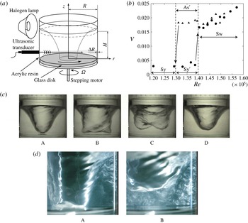
Figure 1(a) shows a schematic of the experimental set-up. The details of the experimental set-up are available in Tasaka & Iima (Reference Tasaka and Iima2009) and only a summary is presented here. An open-ended cylindrical vessel with an inner radius of
 $R=42$
mm was filled with a liquid (tap water). The liquid was driven by a rotating glass disk mounted on the bottom of the cylinder and connected to a stepping motor through a shaft. A gap of
 ${\rm\Delta}R=0.3$
mm was left between the disk and the sidewall of the vessel (the disk–rim gap). The height of the liquid at rest,
 $H$
, was 40 mm, and the aspect ratio
 $\mathscr{A}=H/R$
was 0.95. The values of
 $R$
and
 $\mathscr{A}$
were close to those used in Suzuki et al. (Reference Suzuki, Iima and Hayase2006) and Tasaka & Iima (Reference Tasaka and Iima2009). In the present study, the rotation speed of the disk,
 ${\it\Omega}$
, was varied between 300 and 850 r.p.m. (5.00 and 14.2 Hz), and
 $Re$
between
 $0.55\times 10^{5}$
and
 $1.57\times 10^{5}$
. As suggested in Suzuki et al. (Reference Suzuki, Iima and Hayase2006) and Tasaka & Iima (Reference Tasaka and Iima2009),
 $Re$
was used to describe the flow structure and the free surface. We remark that the Froude number
 $Fr=2{\rm\pi}{\it\Omega}R/(gH)^{1/2}$
, the ratio between the centrifugal acceleration and the gravity, is also an important parameter. In the parameter range of this paper, however,
 $Fr$
is proportional to
 $Re$
because we control
 ${\it\Omega}$
alone and
 $Fr$
is represented as
 $Fr={\it\nu}/\{(gH)^{1/2}R\}Re\;(=3.80\times 10-5[3.80\times 10^{-5}Re]Re)$
.
(a) Experimental set-up. (b) Intensity of velocity fluctuation
 $V$
versus
 $Re$
. With increasing
 $Re$
,
 $V$
suddenly increases at
 $Re=1.4\times 10^{5}$
(
 $Fr=5.3$
). With decreasing
 $Re$
, a relatively high intensity of velocity fluctuation is maintained until
 $Re=1.3\times 10^{5}$
(
 $Fr=4.9$
). (c) Process of surface switching. A: Symmetric surface shape. B: Loss of axisymmetry of state A. C: After state B, the surface height increases and two humps appear. The new shape rotates temporarily. D: Axisymmetry is restored after state C, and the surface then elongates, resulting in the restoration of state A. This cycle is not time-periodic. (d) Visualisations of the flow during surface switching using fine flakes (
 $Re=1.46\times 10^{5}$
) (
 $Fr=5.55$
). A: Flow in state TA (the state between A and B in (c)). B: Flow in state RO (corresponding to C in (c)).

UVP was used to obtain the instantaneous velocity profiles along the line of propagation of the ultrasonic waves. The use of UVP enabled acquisition of the spatio-temporal fluid velocity data. An ultrasonic transducer was mounted on the sidewall of the vessel at a height
 $z$
, 8 mm above the disk (
 $z/H=0.2$
). The instantaneous profiles of the radial velocity component along the horizontal centreline of the cylinder,
 $u(r,t)$
, were measured through the sidewall. The spatial resolution of the velocity profile was 0.74 mm. The spatial distribution of the intensity of the temporal velocity fluctuation,
 $u_{sp}(r)=[(1/T)\int _{0}^{T}u^{\prime }(r,t)^{2}\,\text{d}t]^{1/2}$
(where
 $u^{\prime }(r,t)$
is the fluctuating component of
 $u(r,t)$
and
 $T$
is the measurement time), was calculated to describe the flow transition with respect to
 $Re$
. The time series of the spatial root mean square of
 $u^{\prime }(r,t)$
,
 $u_{rms}(t)=[1/(({\it\eta}_{2}-{\it\eta}_{1})R)\int _{{\it\eta}_{1}R}^{{\it\eta}_{2}R}u^{\prime }(r,t)^{2}\,\text{d}r]^{1/2}$
 $({\it\eta}_{1}=0.49,{\it\eta}_{2}=0.67)$
, was also used to quantitatively describe the dynamic switching. In this paper, we define the intensity of velocity fluctuation as
 $V=1/(2{\rm\pi}{\it\Omega}R({\it\eta}_{1}-{\it\eta}_{2}))\int _{{\it\eta}_{1}R}^{{\it\eta}_{2}R}u_{sp}(r)\,\text{d}r$
to characterise the flow structure. The free surface of the water was captured by a digital video camera at 29.97 f.p.s., and the surface height
 $h(t)$
was extracted from the shots.
2.2. Known results of surface switching
Several measurements have been performed on the surface switching phenomena (Suzuki et al. Reference Suzuki, Iima and Hayase2006; Tasaka et al. Reference Tasaka, Iima and Ito2008a ,Reference Tasaka, Ito and Iima b ; Tasaka & Iima Reference Tasaka and Iima2009; Iima et al. Reference Iima, Iijima, Sato and Tasaka2011). Below, we briefly summarise previous findings from studies that have been published in journals and conference proceedings as well as abbreviations used in the present analysis to clarify what is already known and what will be discussed in this subsection. In the following sections, new results will be presented and discussed.
Figure 1(b) is a bifurcation diagram of a flow transition characterised by the intensity of velocity fluctuation (Tasaka & Iima Reference Tasaka and Iima2009). When
 $Re<1.3\times 10^{5}(Fr<4.9)$
, the surface shape is axisymmetric, although it elongates vertically as
 $Re$
is increased. This state is termed Sy. For
 $1.3\times 10^{5}<Re<1.4\times 10^{5}$
(
 $4.9<Fr<5.3$
), the surface remains axisymmetric and in contact with the bottom, although intermittent oscillation of the surface shape is observed. This state is termed
 $\text{Sy}^{\prime }$
. The amplitude of the oscillation increases with increasing
 $Re$
, and the fluid ultimately detaches from the bottom, resulting in surface switching (Tasaka et al.
Reference Tasaka, Ito and Iima2008b
).
For
 $Re>1.6\times 10^{5}$
(
 $Fr>6.1$
), the surface shape loses its axisymmetry and exhibits an
 $m=2$
symmetry. The surface then rotates at almost constant speed with a period of
 $O(0.1~\text{s})$
and its shape is observed to oscillate with a longer period of 6–7 s. This state is termed As. When the rotation speed is decreased, hysteresis occurs within
 $1.3\times 10^{5}<Re<1.4\times 10^{5}$
(
 $4.9<Fr<5.3$
) and a state different from state As is observed. In this state, the surface shape has an
 $m=2$
symmetry, as in state As, but there is no obvious oscillation of the surface height with a longer period (Tasaka & Iima Reference Tasaka and Iima2009). This state is termed
 $\text{As}^{\prime }$
.
Surface switching (Sw; Suzuki et al.
Reference Suzuki, Iima and Hayase2006) is observed for
 $1.4\times 10^{5}<Re<1.6\times 10^{5}$
(
 $5.3<Fr<6.1$
). In this state, the surface shape is non-stationary; the backlight projection photographs in figure 1(c) show the typical temporal sequence of the change of the surface shape. The temporal change is non-periodic. Detailed analysis suggests that the surface transits through a state similar to As (termed (quasi-)regular oscillation (RO)), a state similar to
 $\text{As}^{\prime }$
(termed flat rotation (FR)), and dynamic transitions between RO and a state in which the free surface descends and almost recovers the axisymmetry (termed temporary axisymmetric state (TA)). This transition is termed laminar–turbulent switching (LTS). The detailed characteristics of these states are discussed in Tasaka & Iima (Reference Tasaka and Iima2009). The surface shape in state RO has clear humps, as shown for state C of figure 1(c). It has two time scales and is also characterised by periodic modification, vertical surface height oscillation, and rotation. The surface shape in state FR neither has significant humps nor exhibits significant periodic modification (Tasaka & Iima Reference Tasaka and Iima2009; see also § 3.1).
Figure 1(b) shows that the upper branch is formed by states with higher values of
 $V$
; hence, the upper branch is here termed the high-intensity branch.
In a previous study (Tasaka et al. Reference Tasaka, Ito and Iima2008b ), the flow during the Sw sequence was visualised by fine flakes (figure 1 d). It was observed that, in the TA state, the flow was laminar, with the exception of in the near-surface region. However, the flow was observed to be wholly turbulent when the surface detached from the bottom, and the condition was similar to state FR or RO (Tasaka et al. Reference Tasaka, Ito and Iima2008b ). Thus, the flows of the states in the high-intensity branch were either strongly mixing or turbulent, except the transient laminar state (TA) in the Sw region. Tasaka et al. (Reference Tasaka, Ito and Iima2008b ) reported that disturbances in both the central region and the near-wall region immediately spread after the detachment of the surface from the bottom. The results revealed that an increase in the asymmetry of the surface shape preceded the spreading of the turbulent flow.
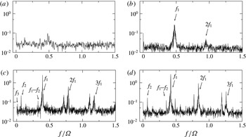
Power spectrum of velocity fluctuation normalised by
 $(2{\rm\pi}{\it\Omega}R)^{2}\times 10^{-6}$
. (a) Sy region (
 $Re=1.29\times 10^{5}$
); (b)
 $\text{Sy}^{\prime }$
region (
 $Re=1.37\times 10^{5}$
); (c) Sw region (
 $Re=1.57\times 10^{5}$
); (d)
 $\text{As}^{\prime }$
region (
 $Re=1.36\times 10^{5}$
).

Judging from the wholly disturbed flow by visualisation (figure 1
d), and the fact that
 $Re$
is close to the critical value for the laminar–turbulent transition of the boundary layer, the flow state is suggested to be turbulent. However, whether the turbulence is developed or not has not been quantified, because the frequency of the UVP detector is
 $1/13~\text{m s}^{-1}$
, which is too coarse to check the power law for the velocity fluctuation. Therefore, we use the term ‘turbulence’ for this flow state for simplicity, but we should be careful to consider the effect intrinsic to turbulence in this system.
The power spectra of the velocity fluctuation,
 $P(Re;f)$
, are shown in figure 2 (Tasaka et al.
Reference Tasaka, Iima and Ito2008a
). They consist of peaks at
 $f=f_{1}$
,
 $f_{2}$
and
 $f_{3}$
(
 $f_{1}>f_{2}>f_{3}$
) and their combinations. We note that
 $P(Re;f_{1})>P(Re;f_{2})>P(Re;f_{3})$
; that is,
 $f_{1}$
corresponds to the major peak. In the
 $\text{Sy}^{\prime }$
region (figure 2
b),
 $f_{1}$
corresponds to the frequency of the intermittent oscillation caused by interfacial instability (Tasaka et al.
Reference Tasaka, Iima and Ito2008a
,Reference Tasaka, Ito and Iima
b
).
However, the details of the transition dynamics are still unclear. We note that the thicknesses of the boundary layer on the disk (the Ekman layer, estimated by
 $\sqrt{{\it\nu}/2{\rm\pi}{\it\Omega}}$
) and that on the sidewall (the Stewartson layer, estimated by (
 $({\it\nu}/2{\rm\pi}{\it\Omega}R^{2})^{1/3}R$
) are both
 $O(0.1)$
mm, which is much smaller than the container size (
 $R=42$
mm). It is therefore necessary to clarify the bulk flow structure with respect to the mechanism of the transition through the states. This was done in the present study using the flow distribution obtained by UVP and analysis of the surface shape.
3. Transitions of flow pattern with changing rotation speed
3.1. Frequency transition for changing rotation speed
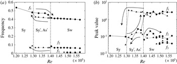
(a) Peak frequencies of the power spectrum as functions of
 $Re$
. The frequencies are non-dimensionalised by
 ${\it\Omega}$
. The solid circles indicate the values measured with increasing
 $Re$
, and the solid triangles the values measured with decreasing
 $Re$
. Hysteresis is observed for
 $f_{1}$
. (b) Peak values of the power spectrum as functions of
 $Re$
. The symbols are as in (a). Hysteresis is observed for
 $f_{1}$
. For
 $1.3\times 10^{5}<Re<1.4\times 10^{5}$
(
 $4.9<Fr<5.3$
), a mode with frequency
 $f_{2}$
is observed only for the case of decreasing
 $Re$
(state
 $\text{As}^{\prime }$
).

In this section, we discuss the transitions of the flow based on the peaks of the power spectrum. The changes of the peak frequencies and their values in the typical states will be useful in discussing the dynamics of the flow structures, including the surface switching.
Figure 3(a) shows that
 $f_{1}$
does not change significantly in the Sy and
 $\text{Sy}^{\prime }$
regions, and also in the Sw region, although it decreases when the state changes from
 $\text{Sy}^{\prime }$
to Sw. This mode corresponds to the rotation of the non-axisymmetric surface shape, as previously observed in the power spectrum of the surface height
 $h(t)$
(Suzuki et al.
Reference Suzuki, Iima and Hayase2006). However, the strength of the
 $f_{1}$
mode increases significantly during this transition, as evidenced by
 $P(1.4\times 10^{5};f_{1})/P(1.3\times 10^{5};f_{1})>10$
(figure 3
b). The magnitude and frequency of this mode are less dependent on
 $Re$
in states Sw and
 $\text{As}^{\prime }$
. The values of
 $f_{1}$
indicate the occurrence of hysteresis (figure 3
a,b). The increase of the
 $f_{1}$
mode in state
 $\text{Sy}^{\prime }$
suggests that the corresponding flow, which comprises intermittent oscillation, becomes significant and finally triggers the surface switching. The flow in this region is compared with the predictions of the theory of Tophøj et al. (Reference Tophøj, Mougel, Bohr and Fabre2013) in § 3.2. The interface instability by itself does not produce a global mixing flow because the intensity of velocity fluctuation does not increase significantly (figure 1
b). A similar process is observed in the dynamics of the surface detachment in surface switching. In this case, no globally disordered flow is observed while the interface oscillation grows; however, such becomes visible at the moment that the interface detaches from the bottom (Tasaka et al.
Reference Tasaka, Ito and Iima2008b
).
When
 $Re$
decreases, the peak value of
 $f_{1}$
does not decrease but rather increases (figure 3
b). The frequency
 $f_{1}$
varies linearly in this regime (figure 3
a). In contrast, the peak value of
 $f_{2}$
decreases with decreasing
 $Re$
, and the value drops off sharply near the critical point. The frequency
 $f_{2}$
corresponds to the longer period of 6–7 s observed in the relatively slower vertical oscillations. The rate of the kinetic energy input by the rotating bottom is proportional to
 $Re$
(or
 ${\it\Omega}$
). However, when
 $Re$
is lower than a critical value, the turbulent flow can no longer be maintained and there is a transition to laminar flow. An ordered rotating flow subsequently develops, resulting in the generation of a pressure gradient, and consequently a reduction in the pressure in the central region. Thus, the surface elongates and touches the bottom, ultimately establishing state Sy.
3.2. Intermittent oscillation in
 $\text{Sy}^{\prime }$
region and comparison with the theory of Tophøj et al. (Reference Tophøj, Mougel, Bohr and Fabre2013)

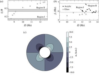
(a) Radius of the surface shape at the bottom,
 ${\it\xi}$
, as a function of
 ${\it\Omega}$
. The two grey bands indicate the unstable regions of
 ${\it\xi}$
for
 $m=2$
(Mougel et al.
Reference Mougel, Fabre and Lacaze2014). (b) Frequencies of the intermittent oscillation of the surface shape. The open diamonds correspond to the glass disk and the solid squares correspond to the acrylic disk. The two lines indicate the frequencies of the unstable modes for
 $m=2$
. (c) Field of
 $u_{r}$
based on the theory of Tophøj et al. (Reference Tophøj, Mougel, Bohr and Fabre2013). The two circles indicate
 $r={\it\xi}$
and
 $R$
, respectively.

In this section, we compare the results of the stability theory of a swirling free-surface flow proposed by Tophøj et al. (Reference Tophøj, Mougel, Bohr and Fabre2013) with our experimental observations. Mougel et al. (Reference Mougel, Fabre and Lacaze2014) used the theory to predict the instability regions and modes for the same parameters as in our experimental set-ups. They found that the occurrence of the
 $m=2$
mode was significant in the regions
 $0.16<{\it\xi}/R<0.18$
(hereafter referred to as region I) and
 $0.26<{\it\xi}/R<0.29$
(hereafter referred to as region II), where
 ${\it\xi}$
is the radius of the cross-section of the surface shape at the bottom. The corresponding dimensional frequency ranges of the mode were determined to be
 $5.7<f<5.9$
Hz in region I and
 $6.8<f<6.9$
Hz in region II.
In our experiment, state
 $\text{Sy}^{\prime }$
was observed to be characterised by an axisymmetric surface shape with intermittent oscillation. In this regime, the intermittent oscillation does not grow and the surface shape assumes its axisymmetry soon after the oscillation begins. We therefore posit that the oscillation is caused by the instability of the swirling flow and here compare our experimental measurements with the theoretically predicted values. Figure 4(a,b) show the measured values of
 ${\it\xi}$
and
 $f_{1}$
, respectively. The frequencies for the acrylic disk, which produced a wide range of values in state
 $\text{Sy}^{\prime }$
(Tasaka et al.
Reference Tasaka, Iima and Ito2008a
), are also shown. The oscillation was observed to occur for
 ${\it\Omega}>10.0$
Hz and
 ${\it\xi}/R>0.31$
. The value of
 ${\it\xi}$
at the onset of the oscillation is close to region II. In this range, the trend of the frequency
 $f_{1}$
is similar to that close to region I. If
 ${\it\Omega}$
is decreased to 8.67 Hz, the value of
 ${\it\xi}$
would fall inside region I. However, as far as the experimental observations are concerned, the measured values at the onset of the oscillation deviate from the theoretically predicted values. Considering the simplicity of the theory with regard to the potential flow and two-wave resonance, we conclude that the assumptions produce at least qualitatively reasonable values compared to our experimental observations. In § 4.1, we discuss the swirling flow velocity distribution, which we consider as the possible reason for the discrepancies between the experimental results and theoretical predictions.
The theoretically obtained radial distribution of the swirling flow velocity is shown in figure 4(c) for
 $m=2,f=6.8$
Hz and
 ${\it\xi}/R=0.3$
, which are typical values in region II. The details are explained in appendix A. The flow distribution shows a relatively large amplitude near the surface
 $r={\it\xi}$
, and that the amplitude decreases with increasing
 $r$
. The distribution is compared with those obtained by experiments in §§ 4 and 5.
4. Flow structure for (temporary) rotating states
In this section, we focus on the temporary rotating states. In § 4.1, we show the swirling flow distribution in the
 $\text{Sy}^{\prime }$
state to discuss the assumption in the theory by Tophøj et al. (Reference Tophøj, Mougel, Bohr and Fabre2013). Then, we proceed to the analysis of the flow structure during surface switching. We focus on the FR state (§ 4.2) and the RO state (§ 4.3), before analysing the LTS event in § 5.
4.1. Swirling flow distribution
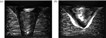
Photograph of particle paths taken from the side. (a)
 ${\it\Omega}=700$
r.p.m. (11.7 Hz), (b)
 ${\it\Omega}=800$
r.p.m. (13.3 Hz).

(a) Scatter diagram of the estimated set
 $(r,u_{{\it\theta}})$
(
 ${\it\Omega}=700~\text{r.p.m.}$
(11.7 Hz)). (b) Snapshot of the container from the side showing the surface shape.

We estimate the swirling velocity distribution by the particle tracking method using porous resin particles (radius
 ${\approx}\!100~{\rm\mu}\text{m}$
, specific gravity
 $=$
1.01). Figure 5 shows the particle paths for
 ${\it\Omega}=700$
and 800 r.p.m. (11.7 and 13.3 Hz).
To analyse the swirling velocity, we considered the cylindrical coordinate
 $(r,{\it\theta},z)$
and defined
 ${\it\theta}=0$
so that the right half of the photograph corresponded to the
 $r{-}z$
plane. A particle was tracked to obtain its coordinates when the projection of its orbit on the photograph attained a local maximum or minimum in the horizontal direction; that is, when
 $(r,{\it\theta},z,t)=(r_{1},{\it\theta}_{1},z_{1},t_{1})$
, where
 ${\it\theta}_{1}=0$
and
 ${\rm\pi}$
for the maximum and minimum values, respectively. We then measured the time
 $t=t_{2}({<}t_{1})$
at which the same particle passed through the middle of the container in the photograph. At the time
 $t=t_{2}$
, the particle passed through the
 $r{-}z$
plane defined by
 ${\it\theta}={\it\theta}_{1}-{\rm\pi}/2$
. The swirling velocity
 $u_{{\it\theta}}$
at
 $r=r_{1}$
was estimated using
 $$\begin{eqnarray}u_{{\it\theta}}=\frac{{\textstyle \frac{1}{2}}{\rm\pi}r_{1}}{t_{1}-t_{2}}.\end{eqnarray}$$
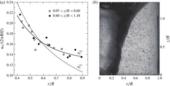
Figure 6(a) shows the scatter diagram of the estimated set
 $(r,u_{{\it\theta}})$
for the case
 ${\it\Omega}=700$
r.p.m. (11.7 Hz). It should be noted that, if
 $u_{{\it\theta}}\propto r$
, the flow is a rigid-body rotation (or a flow with uniform vorticity), and if
 $u_{{\it\theta}}\propto r^{-1}$
, the flow is a potential flow, which is used as the basic flow of the theory of Tophøj et al. (Reference Tophøj, Mougel, Bohr and Fabre2013). The symbols in the figure are classified with respect to their
 $z$
components as lower position (open circle,
 $0.07<z/H<0.60$
) and higher position (solid circle,
 $0.60<z/H<1.18$
). To check whether the flow distribution was well represented by the potential flow assumed by Tophøj et al. (Reference Tophøj, Mougel, Bohr and Fabre2013), we used the following two fitting functions:
 $$\begin{eqnarray}\left(\frac{u_{{\it\theta}}^{(1)}(r)}{2{\rm\pi}R{\it\Omega}}\right)=a_{1}\left(\frac{r}{R}\right)^{-1},\quad \left(\frac{u_{{\it\theta}}^{(2)}(r)}{2{\rm\pi}R{\it\Omega}}\right)=a_{2}\left(\frac{r}{R}\right)^{-1}+b_{2}\left(\frac{r}{R}\right).\end{eqnarray}$$
Equation (4.2a
) represents a potential flow used in the theory of Tophøj et al. (Reference Tophøj, Mougel, Bohr and Fabre2013), whereas (4.2b
) incorporates a rigid-body rotation flow in addition to the potential flow. We used both functions for the fitting. The best fitted curves for
 $u_{{\it\theta}}^{(1)}(r)$
and
 $u_{{\it\theta}}^{(2)}(r)$
(
 $a_{1}=0.0956,a_{2}=0.0769,b_{2}=0.0560$
) are the solid and broken curves, respectively. It is clear that the potential flow alone is not sufficient to represent the azimuthal flow distribution, and the superposition of a rigid-body rotation flow and the potential flow yields a reasonable representation of the flow distribution. Note that Fabre & Mougel (Reference Fabre and Mougel2014) considered different models, in which the base flow was separated into a strictly potential region and a rigid-body rotation region. Moreover, the fitted curve
 $u_{{\it\theta}}^{(2)}(r)$
seems to represent the measured points in both the lower and higher positions, suggesting that the azimuthal flow distribution does not depend significantly on the height.
If the sidewall rotates at the same angular speed as the endwall, the azimuthal velocity distribution simply becomes a rigid-body rotation flow. In our set-up, the major part of the azimuthal velocity is represented by the potential flow, but a rigid-body rotation component remains. We remark that the two terms on the right-hand side of (4.2b
) have the same value at
 $\displaystyle r=R\sqrt{a_{2}/b_{2}}=1.17R$
, which is outside the cylinder. Therefore, the potential flow is major inside the cylinder. The rigid-body rotation term is expected to shift the detailed parameter ranges of the instability and frequencies discussed in § 3.2.
Figure 5(b) shows the case of
 ${\it\Omega}=800$
r.p.m. (13.3 Hz). Although the particle paths suggest a relatively strong vertical flow, the major directions of the particle paths can still be observed to be horizontal, indicating that
 $u_{{\it\theta}}$
is large. However, the discernible randomness of the paths also suggests strong mixing. To examine the flow structure, it is necessary to obtain the spatial flow distributions. This is discussed in the following sections.
4.2. Flow structure in FR state
In this section, we analyse the temporary rotating state during surface switching, namely, the FR state, so called because the flow is regular compared to the other states with asymmetric surface shapes (Tasaka & Iima Reference Tasaka and Iima2009). We use Taylor’s frozen hypothesis to define the two-dimensional flows associated with the results of the UVP.
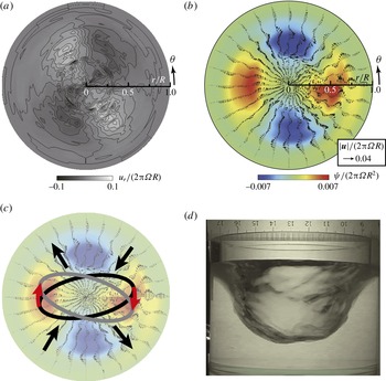
The flow distributions in the FR state are shown in figure 7(a), where the spatio-temporal data
 $u_{r}(r,t)$
obtained by UVP analysis is mapped to the two-dimensional field of the radial velocity
 $\hat{u} _{r}(r,{\it\theta})=u_{r}(r,2{\rm\pi}(t-t_{0})/{\it\tau})$
based on Taylor’s frozen hypothesis. Here,
 $t_{0}$
is the start time of the measurement and
 ${\it\tau}$
is the period of the surface shape rotation, which was estimated by two periods of
 $u_{r}$
oscillation. The rotation direction is counterclockwise.
Although the radial velocity field represents the flow structure, it is not convenient for use in determining global flow structures such as vortices with sizes comparable to that of the container. We therefore defined an associated flow as a two-dimensional incompressible fluid with a radial flow component that corresponds to
 $\hat{u} _{r}(r,{\it\theta})$
, and zero mean azimuthal velocity along any circle centred at
 $r=0$
. The detailed definition of the associated flow is given in appendix B. Because these assumptions do not generally hold, the associated flow is not always the actual flow field on the horizontal cross-section. However, we expect that the field would represent a secondary flow superposed on the base flow discussed in § 4.1, and this would particularly constitute a perturbation of the base flow, which is two-dimensional according to the theory of Tophøj et al. (Reference Tophøj, Mougel, Bohr and Fabre2013). The associated flow field of that shown in figure 7(a) is shown in figure 7(b). Here, the entire flow structure, including the surface, rotates clockwise and the horizontal cross-section of the surface is elongated laterally (parallel to the line
 ${\it\theta}=0,{\rm\pi}$
; see figure 7
d).
(a) Distribution of
 $u_{r}$
in the FR state. (b) The associated two-dimensional flow field. The colours indicate the stream function. (c) Schematic of the surface deformation and local flow. (d) Picture of the surface taken from the side (from the bottom of (a) and (b)).

There is a direct connection between the radial flow field in figure 7(a) and the associated flow structure. This consists of quadrupole vortices comprising two positive and two negative vortices. As shown in figure 7(a), the radial flow direction is towards the centre around
 ${\it\theta}\approx {\rm\pi}/4,5{\rm\pi}/4$
and off the centre around
 ${\it\theta}\approx 3{\rm\pi}/4,7{\rm\pi}/4$
. The foregoing regions are those between adjacent vortices of different signs and are indicated by arrows in figure 7(c). The stream function of the associated flow thus gives direct insight into the structure of the secondary flow.
This vortex structure can cause a clockwise rotation of the surface shape. In figure 7(c), a schematic of the horizontal cross-section is superposed on the flow field. The dynamics of the cross-section of the surface is indicated by two ellipses; the grey ellipse represents the surface shortly after that represented by the black ellipse. If we assume that the radial flow pattern is almost constant in the
 $z$
-direction, the surface shape would be squeezed around
 ${\it\theta}\approx {\rm\pi}/4,5{\rm\pi}/4$
and stretched around
 ${\it\theta}\approx 3{\rm\pi}/4,7{\rm\pi}/4$
. Such deformations cause a rotation of the surface in a clockwise direction, and the flow itself is not a simple constant rigid-body rotation. The flow field is similar to that in figure 4(c), which is caused by a centrifugal wave, based on the theory of Tophøj et al. (Reference Tophøj, Mougel, Bohr and Fabre2013), although the flow field consists of quadrupole vortices, unlike the potential flow shown in figure 4(c).
4.3. Flow structure in the RO state
(a) Snapshot of the distribution of
 $u_{r}$
in an RO with a large surface height (ROh). (b) Snapshot of the distribution of
 $u_{r}$
in an RO with a small surface height (ROl). (c) The associated flow vector and stream function for ROh. (d) The associated flow vector and stream function for ROl. (e) Photograph of ROh from the side. (f) Photograph of ROl from the side.

In the RO state, the surface shape has an
 $m=2$
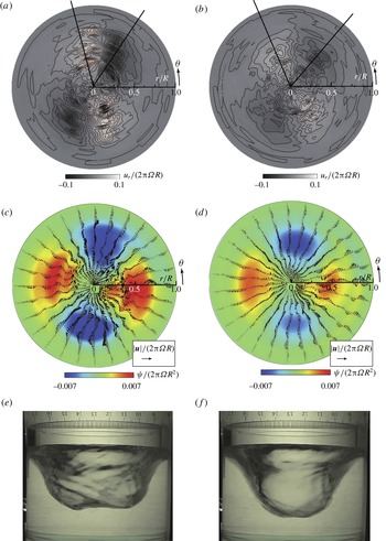
symmetry and rotates at a constant speed with a vertical oscillation that has a longer period of 7–8 s. In the vertical oscillation, two clear humps can be observed at the bottom of the surface when the surface height is high (ROh), but the humps are less obvious when the surface height is low (ROl). The flow structures of these two states are shown in figure 8.
Figure 8(a,b) show the radial velocity distributions for the ROh and ROl states, respectively. The flow structures are similar to those of the FR state, although the flow speed is higher in the ROh state, where two humps are distinct. The peak of the radial flow in the ROl state is roughly half of that in the ROh state. The associated flows of the ROh and ROl states are shown in figure 8(c,d), respectively. As can be deduced from the radial velocity fields, the quadrupole structure of the ROh state is stronger than that of the ROl state. These particular photographs were selected because their sequences were the most periodic, and the discontinuities at
 ${\it\theta}=0$
are therefore not distinct. In some of the other photographs, the discontinuities are obvious because of the long-period oscillations with the characteristic frequency of
 $f_{2}$
(figure 3). The surface shape pictures of the ROh and ROl states are shown in figure 8(e,f), respectively. The long axis of the horizontal cross-section is parallel to the line
 ${\it\theta}=0,{\rm\pi}$
as in the FR case.
5. Dynamical flow change during surface detachment
Graphs of
 $h/H$
and
 $r_{i}/R$
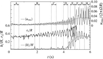
during the period including the TA state, the detachment of the surface from the bottom, and the convergence to the RO state. The time series of
 $\langle h\rangle$
and
 $\langle u_{rms}\rangle$
were obtained using a 0.53 s moving average of
 $h$
and a 0.52 s moving average of
 $u_{rms}$
, respectively. Moving averages were used in order to eliminate the short-term fluctuations in
 $h$
and
 $u_{rms}$
.

Spatial distribution of
 $u_{r}$
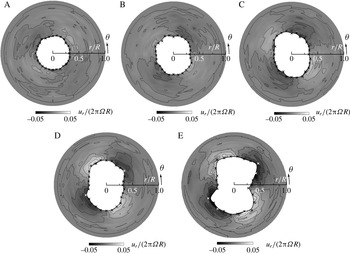
and the interface positions of the cross-sections of the surface during the detachment of the surface from the bottom at the occurrence of surface switching. The alphabetic identifiers of the figure panels correspond to the time intervals in figure 9. The axisymmetry of the interface and flow is gradually lost, and the surface detachment occurs between D and E.

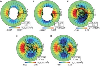
Associated flows of the transient processes of surface deformation, surface detachment, and convergence to the state similar to the RO state. The alphabetic identifiers of the figure panels correspond to the time intervals in figure 9.

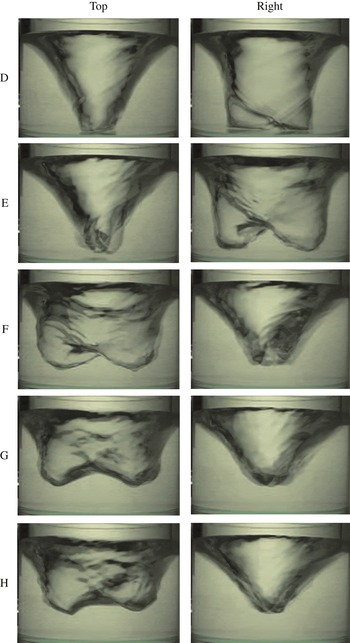
Photographs taken from the side during the process of the surface detachment. The alphabetic identifiers of the figure panels correspond to the time intervals in figure 9. The photographs in the ‘top’ column show the surface looking from the top of the figures in figure 11, and those in the ‘right’ column show the surface looking from the right.

In this section, we focus on the surface-detachment process of the LTS event during surface switching, in which a drastic change of the flow structure and surface shape is observed. The detailed dynamics of the surface detachment during surface switching is illustrated in figures 9 and 10 for the Sw region, where
 $Re=1.46\times 10^{5}$
(
 $Fr=5.55$
).
Figure 9 shows the time series of the surface height
 $h(t)$
and the radial distance to the air–water interface
 $r_{i}(t)$
, which was determined using the algorithm developed by Murai et al. (Reference Murai, Tasaka, Nambu, Takeda and Gonzalez2010). It should be noted that the local maximum of
 $r_{i}(t)$
corresponds to half of the width of the surface shape at the measured height. The air–water interface is initially almost circular, but the axisymmetry is gradually lost. Figure 10 shows the air–water interfaces and
 $u_{r}$
distributions at intervals A–E. Generally, the magnitude of
 $u_{r}$
is larger near the interface and decreases with increasing
 $r$
. This type of spatial distribution of
 $u_{r}$
is qualitatively similar to that in figure 4(c). The similarity is because the major part of the background flow in both cases comprises only the azimuthal component. This velocity distribution accompanies non-closed streamlines that qualitatively correspond to those of the centrifugal wave in the theory of Tophøj et al. (Reference Tophøj, Mougel, Bohr and Fabre2013). Within the scope of this theory, the streamlines never close, because of the assumption of potential flow. However, in the present study, closed streamlines were observed in the cases of RO and FR, and the developed non-axisymmetric perturbations of states similar to RO are shown in figures 9 and 10.
The associated flow fields corresponding to figure 10 are presented in figure 11, which for interval D shows a quadrupole vortex as in the RO and FR cases, except at the existence of the air–water interface. It should be noted that the longer axis of the cross-section of the surface shape is now vertical or parallel to the line defined by
 ${\it\theta}={\rm\pi}/2,3{\rm\pi}/4$
.
Just after the detachment of the free surface from the bottom, the cross-section assumes a more complicated shape, although the flow patterns remain qualitatively the same (see interval E in figures 10 and 11). During the process of the surface detachment from the bottom, the amplitude of the oscillation of
 $r_{i}(t)$
increases, and the oscillation of
 $h(t)$
becomes apparent after the detachment. Just after the detachment, the oscillations of
 $h(t)$
and
 $r_{i}(t)$
are in-phase and the surface shape shown for state C in figure 1(c) is assumed.
The post-detachment process occurs in interval F, wherein the surface shape converges to the quasiperiodic state similar to that of RO. Interval F in figure 9 shows only two peaks of
 $u_{rms}$
, while the other intervals have four peaks. The two-peak property in interval F suggests that only two vortices (positive and negative) are present during this period, unlike during intervals A–E. Actually, the associated flow in the interval F (figure 11) shows two major vortices, although they are elongated in the azimuthal direction. We also note that the associated flow is discontinuous at
 ${\it\theta}=0$
, which is because the flow periodicity does not hold, not even approximately.
During the convergence process, the flow field recovers a
 $m=2$
symmetry as shown in figure 11 (intervals G and H). Smaller vortices can be observed near the central part in addition to the major quadrupole vortices (interval G in figure 11). However, these vortices disappear until the convergence is completed. In interval H, the flow field is now similar to that in the RO state and the direction of the longer axis of the surface cross-section is now parallel to the line
 ${\it\theta}=0,{\rm\pi}$
as in the RO state.
It is, however, surprising that the cross-section rotates by
 $-{\rm\pi}/2$
during the convergence process; i.e. from the state in which the surface touches the bottom to the state similar to the RO state. Nevertheless, the two states appear similar. The photographs in figure 12 show the typical surface shapes during intervals D–H. It is clear that the longer axis of the cross-section rotates between intervals E and F. This suggests that the relationship between the flow structure and the surface shape in the asymmetric state with a dry central region is different from that with a wet central region.
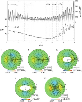
The same as figure 9 but for another period that includes the LTS event, wherein the surface does not touch the bottom. The labels I, J, K, L and M on the lower panels correspond to the intervals in the main panel.

To examine the relationship between the
 ${\rm\pi}/2$
rotation noted above and the attachment of the surface shape to the bottom, we performed a similar analysis for another LTS event in which the surface elongated towards the bottom but did not touch the bottom. Figure 13 shows the sequence of the surface switching of the latter event. Compared to figure 9, the minimum surface height is larger (
 $h/H\approx 0.1$
). The value is still small, but the surface does not attach to the bottom. Because the height of the UVP probe is not sufficiently different from the surface height, the surface detection algorithm used to obtain figure 9 does not work well here. Hence, the longer and shorter axes of the ellipses of K and L in figure 13 were estimated by image analysis. The quadrupole vortex structures and signs of the vortices are the same as those of the sequences shown in figure 11, but the directions of the longer axes are clearly different (the longer axis is the line defined by
 ${\it\theta}=0,{\rm\pi}$
). We thus conclude that the
 ${\rm\pi}/2$
rotation is closely related to the surface attachment.
Bach et al. (Reference Bach, Linnartz, Vested, Andersen and Bohr2014) reported that the hysteresis behaviours when the surface attached to the bottom (they denoted it by ‘dry’) were different from those when the surface was detached from the bottom (denoted by ‘wet’). The difference suggested the possibility of the structures of the relative flows to the surface in the ‘dry’ and ‘wet’ cases being different, even for a polygonal flow. We should, however, bear in mind that their container size and aspect ratios were different from ours.
6. Concluding remarks
We experimentally analysed the dynamics of surface switching, during which transitions between several surface modes occur along with changes in the flow state. We particularly focused on the flow fields obtained by PTV and UVP, as well as the surface heights simultaneously measured by UVP, and integrated the results.
It was observed that the surface changed from an axisymmetric shape to a non-axisymmetric shape with a transition from a laminar state to a turbulent state. The first event of the transition was the instability of the interface as the axisymmetric state became unstable in the region where the surface switching occurred. During the surface switching process, the amplitude of the unstable mode of the axisymmetric state increased until completion of the flow transition to the turbulent state. The characteristic flow field during this process was not simple swirling but one that contained quadrupole vortices that included a radial component. The streamlines of the flow field resembled those of the unstable mode in the potential flow theory (Tophøj et al. Reference Tophøj, Mougel, Bohr and Fabre2013; Mougel et al. Reference Mougel, Fabre and Lacaze2014), although there were no vortices owing to the assumption of potential flow. The surface deformation finally resulted in the detachment of the surface from the bottom of the container. The rotation speed of the non-axisymmetric shape was observed to correspond to the main frequency of the power spectrum, and the detachment of the surface caused a shift in this frequency, indicating the occurrence of surface switching.
During the surface switching, we observed two transient rotating states, namely, regular oscillation (RO) and flat rotation (FR). Our observations suggested the presence of quadrupole vortices in both cases. The strengths of the vortices depended on the state, but no significant differences were observed. The little difference may be attributed to the detailed dynamic properties of the oscillatory period of the RO, which occurs on a slower time scale. When the balance between the energy dissipation and the energy input was almost neutral, the turbulence noise easily changed the slow dynamics from the state of quasisteady surface height to an oscillating state on the slow time scale. The two states corresponded to FR and RO, respectively. We also successfully extracted a one-dimensional map of the surface shape dynamics on the slow scale, and an additional term of the internal noise that can be used to reproduce the qualitative behaviour of the surface switching (Sato, Iima & Tasaka Reference Sato, Iima and Tasaka2010). By this means we confirmed the above hypothesis. The effect of the internal noise on the surface switching was also investigated by varying the disk–rim gap. This subject will be discussed in detail in a forthcoming paper.
The dynamics of the shape of the free surface of a rotating flow has some interesting characteristics other than surface switching and those highlighted by the instability theory. For example, the dynamics of the formation of a polygonal flow was recently reported (Bergmann et al. Reference Bergmann, Tophoj, Homan, Hersen, Andersen and Bohr2011; Bach et al. Reference Bach, Linnartz, Vested, Andersen and Bohr2014). It was noted that, during the formation process, the surface first transiently assumed an axisymmetric shape before switching to the polygonal shape. In addition, transition through polygonal flows with different apexes (Bach et al. Reference Bach, Linnartz, Vested, Andersen and Bohr2014) has also been reported, as well as the observation that an external disturbance also caused similar transitions (Bach et al. Reference Bach, Linnartz, Vested, Andersen and Bohr2014). These reports showed that the states with non-axisymmetric shapes were related to the state with an axisymmetric shape, even if the axisymmetric state was unstable. This behaviour is similar to that of an orbit passing near a saddle. Such a mathematical viewpoint, combined with the flow analysis performed in this study, should be applied in order to obtain a complete understanding of the dynamics of surface switching. Also, we believe that computational study of a rotating flow with a free surface will be possible in the near future. Then, our experimental results will be compared with the computational results, leading to a complete understanding of the flow physics involved in this scenario.
Acknowledgements
This study was partially supported by Core Research for Evolutional Science and Technology (CREST) no. PJ74100011, and Grants-in-Aid for Scientific Research (23540433, 22360105, 21340019).
Appendix A. Flow field of the theory of Tophøj et al. (Reference Tophøj, Mougel, Bohr and Fabre2013)
According to the theory of Tophøj et al. (Reference Tophøj, Mougel, Bohr and Fabre2013), the assumption of a non-axisymmetric surface shape by a rotating fluid with a free surface can be explained by the linear instability of the axisymmetric flow. Mougel et al. (Reference Mougel, Fabre and Lacaze2014) showed that, for the parameters close to those used in the present study (
 $R/H=0.94$
), a major instability occurred in the
 $m=2$
mode. In the present study, we used the following parameters calculated in Mougel et al. (Reference Mougel, Fabre and Lacaze2014):
 ${\it\xi}=0.3R$
and
 ${\it\omega}=2.8/\sqrt{R/g}$
, where
 ${\it\xi}$
is the radius of the intersection circle between the free surface and the bottom, and
 ${\it\omega}$
is the angular frequency of the unstable mode.
Using the formulae in Tophøj et al. (Reference Tophøj, Mougel, Bohr and Fabre2013) and the parameters in § 2.1, we obtained
 ${\it\omega}=42.77$
Hz,
 ${\it\Gamma}=0.08419~\text{m}^{2}~\text{s}^{-1}$
,
 ${\it\Omega}_{{\it\xi}}=84.40$
Hz and
 $g_{c}=89.75~\text{m}^{2}~\text{s}^{-1}$
, where the notations are the same as in Tophøj et al. (Reference Tophøj, Mougel, Bohr and Fabre2013). These parameters and condition (9) in Tophøj et al. (Reference Tophøj, Mougel, Bohr and Fabre2013) give
 $$\begin{eqnarray}\frac{K_{2}}{K_{1}}=-0.1491.\end{eqnarray}$$
The velocity potential corresponding to the mode
 $m$
of the perturbation is
 $$\begin{eqnarray}{\it\phi}(r,{\it\theta},z)=\text{Re}\left[\left\{\left(\frac{r}{R}\right)^{m}+\frac{K_{2}}{K_{1}}\left(\frac{r}{R}\right)^{-m}\right\}\text{e}^{\text{i}(m{\it\theta}-{\it\omega}t)}\right],\end{eqnarray}$$
where
 $\text{Re}$
here means ‘real part of’. We note that the amplitude was not determined due to the linearity.
Appendix B. Definition of an associated two-dimensional flow
If the radial field
 $u_{r}(r,{\it\theta})$
is assumed to be known, an associated two-dimensional incompressible flow can be defined to establish the flow structure as follows. The continuity equation in the polar coordinates is
 $$\begin{eqnarray}\frac{\partial u_{{\it\theta}}}{\partial {\it\theta}}+\frac{\partial }{\partial r}(ru_{r})=0.\end{eqnarray}$$
Integrating (B 1), we obtain
 $u_{{\it\theta}}(r,{\it\theta})$
as
 $$\begin{eqnarray}u_{{\it\theta}}(r,{\it\theta})=u_{{\it\theta}}(r,0)-\int _{0}^{{\it\theta}}\frac{\partial }{\partial r}(ru_{r}(r,{\it\theta}^{\prime }))\,\text{d}{\it\theta}^{\prime }.\end{eqnarray}$$
We then define an associated flow component
 $u_{{\it\theta}}^{\prime }$
as
 $$\begin{eqnarray}\displaystyle u_{{\it\theta}}^{\prime }(r,{\it\theta}) & = & \displaystyle u_{{\it\theta}}(r,{\it\theta})-\frac{1}{2{\rm\pi}}\int _{0}^{2{\rm\pi}}u_{{\it\theta}}(r,{\it\theta}^{\prime })\,\text{d}{\it\theta}^{\prime }\end{eqnarray}$$
 $$\begin{eqnarray}\displaystyle & = & \displaystyle \frac{1}{2{\rm\pi}}\int _{0}^{2{\rm\pi}}\int _{0}^{{\it\phi}}\frac{\partial }{\partial r}(ru_{r}(r,{\it\theta}^{\prime }))\,\text{d}{\it\theta}^{\prime }\,\text{d}{\it\phi}-\int _{0}^{{\it\theta}}\frac{\partial }{\partial r}(ru_{r}(r,{\it\theta}^{\prime }))\,\text{d}{\it\theta}^{\prime }.\end{eqnarray}$$
The associated two-dimensional flow
 $(U_{r},U_{{\it\theta}})$
is defined as
 $(u_{r}(r,{\it\theta}),u_{{\it\theta}}^{\prime }(r,{\it\theta}))$
. The reconstructed field satisfies the two-dimensional continuity equation, i.e.
 $$\begin{eqnarray}\frac{\partial U_{{\it\theta}}}{\partial {\it\theta}}+\frac{\partial }{\partial r}(rU_{r})=0.\end{eqnarray}$$
By this definition, the associated two-dimensional flow does not have a vertical flow component, and the average
 $U_{{\it\theta}}$
in the azimuthal direction is zero.
These characteristics are of course not the same as those of the actual flow, which is three-dimensional. However, as noted in the main part of this paper, a two-dimensional flow that reproduces the observed radial velocity component is useful to a discussion of the flow structure that contributes to the change of the surface shape.
In practical applications, the double integration in (B 4) is performed in a different order, and the average values are obtained.