2. Some related literature

There is a long tradition in central bank studies supporting the argument that CBs should avoid climate-risk issues and focus on traditional targets, such as inflation, employment (output), and financial stability. Some authors believe the private sector should be a major driver of new energy technology, see Aghion et al. (Reference Aghion, Boneva, Breckenfelder, Laeven, Olovsson, Popov and Rancoita2022). However, recently, climate risks and the transition to a low carbon economy, including renewable energy incentives, are also increasingly viewed by some authors as a monetary policy task.

In fact, a growing body of literature defends the use of monetary and financial policies, in addition to existing fiscal policies to support climate transition (Campiglio, Reference Campiglio2016; Coeure, Reference Coeure2018). However, the policy effectiveness of CBs seems to differ depending on the tools used. In addition, market failures are emerging with a long delay, see Chen et al. (Reference Chen, Semmler and Maurer2022) The effects of these policies are not visible for a long time, and may be accelerated by tipping points (Greiner et al. Reference Greiner, Gruene, Semmler, Greiner, Gruene and Semmler2010).

Central banks are also often seen as neutral with respect to credit flows, and thus not able to target credit and financial flows towards climate mitigation and adaptation-oriented investments. However, carbon-intensive financial assets carry long-term climate-related risks that may create higher volatility, and occasional disruptions (Carney, Reference Carney2015; Semmler et al. Reference Semmler, Braga, Lichtenberger, Toure and Hayde2021). Therefore, some authors advocate that CBs should pursue proactive climate mitigation policies. Other authors argue that CBs should be market-neutral and focus on climate risks only as they affect conventional monetary policy goals, including financial instability risks, inflation, and the output gap. For an extensive discussion, see Brunnermeier and Landau (Reference Brunnermeier and Landau2021).

In practice, however, CBs are already implementing instruments to assess climate risks, such as climate stress tests, and helping to channel financial resources to green investments. In March 2021, the Bank of England explicitly announced a climate mandate—see Bailey (Reference Bailey2021)—while the European Central Bank (ECB), in February 2021, created a climate change center to better design its climate agenda—see (ECB, 2021a). These initiatives, and more, are discussed in CBs‘ international networks—such as the NGFS and the Sustainable Banking Network.

Furthermore, a large body of literature on monetary policy discusses the role of Unconventional Monetary Policy (UMP) instruments, or Quantitative Easing (QE), which has so far tended to be market-neutral, without environmental concerns (De Grauwe, Reference De Grauwe2019; Dafermos et al. Reference Dafermos, Gabor, Nikolaidi, Pawloff and van Lerven2020; Papoutsi et al. Reference Papoutsi, Piazzesi and Schneider2021). Yet, a policy orientation that pursues market-neutrality in asset purchases concentrates CBs’ portfolios mostly on fossil fuel assets, as they represent the majority of the existing assets likely to benefit capital costs of carbon-intensive investments (De Santis et al. Reference De Santis, Roos, Hettler and Tamburrini2018; Battiston and Monasterolo, Reference Battiston and Monasterolo2019). This literature also provides evidence that green bonds can hedge investors against market and oil price volatilities,Footnote ⁵ but the impact of CBs policy on prices has not been sufficiently studied yet.Footnote ⁶

Recent papers join the effort to assess green bond performance but also consider other assets—see Hilmi et al. (Reference Hilmi, Djoundourian, Shahin and Safa2021), Bremus et al. (Reference Bremus, Schuetze and Zaklan2021) and Lichtenberger et al. (Reference Lichtenberger, Braga and Semmler2022). There is also an extensive literature on potential hedge benefits from green bonds and CBs impacting green asset returns. In Appendix E, we discuss CBs’ actions concerning climate risk and climate finance, as well as bond purchasing programs. This discussion also covers initiatives in developing economies with its specifities that might also affect monetary policy and climate risks, such as exchange rate dynamics and constraints (Gevorkyan and Khemraj, Reference Gevorkyan and Khemraj2024; Gevorkyan et al. Reference Gevorkyan2023).

In the present paper, we propose a Nonlinear Qudratic Model, NLQ, solved with AMPL algorithms to study CBs’ green climate goals. This model is directly influenced by Gross et al. (Reference Gross, Loungani and Semmler2019), Faulwasser et al. (Reference Faulwasser, Gross, Semmler and Loungani2020), and Chen et al. (Reference Chen, Semmler and Maurer2022). In the model, we allow the use of delays, and explore the effect of CB policies, guided by a finite horizon decision-making process, that allows CBs to consider climate change and climate risks. The model prioritizes multiple goals, including carbon emissions, as well as inflation, output gaps, and credit flows. The inclusion of climate considerations is a novelty in this model that allows for the study of the effect of carbon emission trends and targets.

Green financial and monetary policy goals supported by instruments and operational procedures can in principle allow for more directed green credit financial flows combating carbon emission trends. An example is the use of long-term credit operations on the financial system with “Targeted Longer-Term Refinancing Operations” (TLTROs)—see ECB (2021b). Since 2014, these operations are key to promoting targeted credit and financial flows. This could allow for an active CB policy for climate risks and impacts, if specific operational instruments channel credit and financial flows to green investments with positive externalities, including R&D and renewable energy.

In the spirit of the CBs’ awareness of climate risks, the NGFS network papers (NGFS, 2023) have also suggested operational instruments to achieve a low carbon economy. The NGFS has dealt extensively with monetary policy issues that take into account climate considerations. Given the above mentioned targeted credit flows and following NGFS communications as viable instruments, we deviate here from the position taken in the work by Aghion et al. (Reference Aghion, Boneva, Breckenfelder, Laeven, Olovsson, Popov and Rancoita2022) who posit that CBs play only a negligible role in impacting green technological transition.

But indeed there are significant obstacles. As to our knowledge there is still very little research on specific macro models dealing with the issue of short-term decision horizons, or with the decision and transmission delays of monetary policies. Furthermore, there is no work on the role of mixed stationary and non-stationary macro variables in this context, and how to combine these variables for policy-decision making with multiple goals. Additionally, explicit weights for these objectives should be implemented (in our case, we use weights for climate, macroeconomic, and financial concerns).

3. A multiple objective dynamic model with climate-macro policies

To build relevant components for this endeavor, we first employ an NLQ model to study the macroeconomic effects of CBs’ decisions in an economy facing climate risks. In this NLQ model, CBs can influence the economy by setting the interest rate (the control variable in the proposed model), managing the risk premium and credit flows through UMP, and taking into consideration climate change in their monetary operations by channeling credit flows to certain sectors.Footnote ⁷ The NLQ model also allows the study of CBs’ decisions when multiple objectives hold: inflation, output, financial stability, as well as arising climate risks.

Secondly, a multiple objective dynamic model is proposed and roughly calibrated using the recent economic performance of selected countries. This multiple objective NLQ model with quadratic penalty functions and nonlinear state equations is described in the following subsections by referring to a climate risk variable, the CO2 emissions trend, as a possible non-stationary variable of concern of the CB. In addition, this model deals also with stationary variables, such as the traditional macro variables referring to economic targets: the inflation rate, the output gap, and the credit flows (related to financial stability). In Section 4, we have also included other variables, and in particular the carbon emission trend for econometric studies.

3.1 Climate risks and policies to flatten the emission curve

Next, we present a macro model in which policy makers react to the previously described basic macroeconomic variables, but are also worried about climate risks. As mentioned, our model type is influenced by Gross et al. (Reference Gross, Loungani and Semmler2019), Faulwasser et al. (Reference Faulwasser, Gross, Semmler and Loungani2020), and Semmler et al. (Reference Semmler, Henry and Maurer2022). These authors use an NLQ model, solved by AMPL algorithms, to represent a CB decision problem with multiple goals and the basic state variables: inflation, output gap, and credit flow dynamics.

A type of Taylor Rule is implemented to account for financial stability, including credit flow dynamics as a financial variable.Footnote ⁸ Although inflation targeting models have traditionally used linear approaches, Faulwasser et al. (Reference Faulwasser, Gross, Semmler and Loungani2020) justify using a NLQ model to account for the nonlinear propagation mechanism of credit flows and credit spreads.Footnote ⁹ However, the model used in this paper has both non-stationary and stationary variables. This brings further theoretical modeling benefits, as well as econometric challenges.

3.1.1 A partial dynamic with a non-stationary carbon emission

Since major macro variables are stationary in CB research (or are made stationary to study them over some business cycle time scale), we focus on the non-stationarity of the carbon emissions data. Making the carbon emission variables stationary, on the other hand, would keep CBs from achieving actual international climate goals. As stated by the Paris Agreement, countries should decrease net emissions by half until 2030, and have net-zero emissions by 2050. This is needed to avoid exceeding the carbon budget the earth is able to sustain, see Edenhofer et al. (Reference Edenhofer, Kadner, von Stechow, Schwerhoff, Luderer, Edenhofer, Kadner, von Stechow, Schwerhoff and Luderer2014).

The emissions trend is the new feature of the dynamic decision model and should be discussed first before we present the full dynamic model. Most Integrated Assessment Models (IAMs), such as the Nordhaus Dynamic Integrated Climate-Economy (DICE) model are modified growth models, and in principle are non-stationary. However, most policy oriented dynamic macro models exhibit stationary features, formulated in linearized form as LQ models with a quadratic penalty, and linear state equations, see for example De Groot et al. (Reference De Groot, Mazelis, Motto and Ristiniemi2021). Often, the state variables are stationary, or made stationary through de-trending or first differencing.

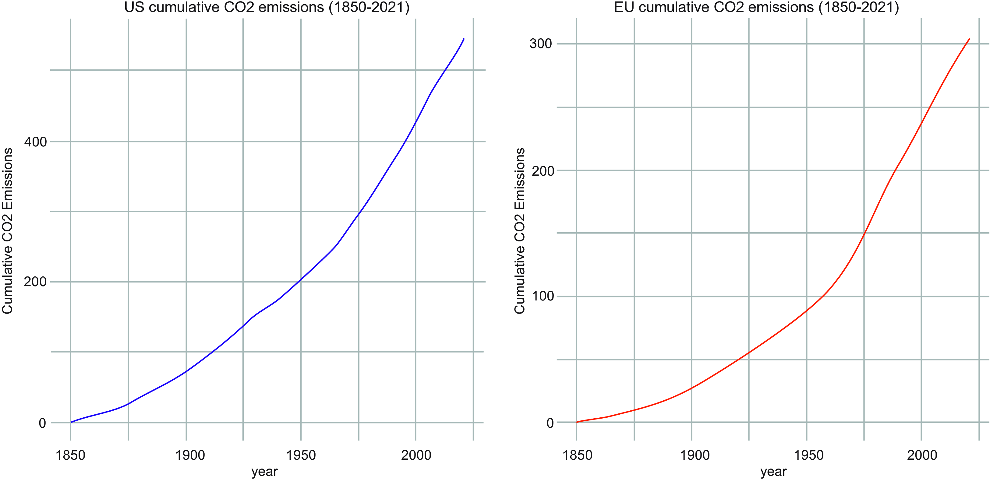
In more formal terms, the literature works with autonomous dynamic systems, meaning autonomous differential equations. In our case, our major concern is the treatment of some non-stationary state variables as state variables. Our dynamic system will thus be a non-autonomous dynamic system, driven in the simplest case by a variable with a time trend. In our case, this concerns mainly the trend in CO2 emissions, since the 1850s, depicted below for the US and Europe in Figure 1.

Figure 1.

Cumulative emissions in Giga tons plotted from 1850 to 2021; LHS carbon emission US; RHS carbon emission Europe, source: Owid-CO2.

Figure 1 shows the annual cumulative CO2 emissions since 1850 for both the USA and all 27 European countries. Since the year 2000, the curves become less steep, with a lower net emission growth rate. However, a huge stock of CO2 has already been emitted since 1850: in the US, roughly 500 billion tons; in the EU, over 300 billion tons. These emissions have contributed to moving the world closer to its carbon budget constraint, which is roughly 400 ppm—for details see Edenhofer et al. (Reference Edenhofer, Kadner, von Stechow, Schwerhoff, Luderer, Edenhofer, Kadner, von Stechow, Schwerhoff and Luderer2014).

Technically, we can represent the type of curve in Figure 1 by a dynamic non-stationary process, leading to a rising stock of carbon in the atmosphere. These processes are then stylized by a non-autonomous differential equation in one variable with time as an independent variable:

(1) \begin{align} \dot {ce}(t)=-\alpha *ce(t)+log(e^{(g_{ce}t)}). \end{align}

Hereby $\dot {ce}(t)$ is the carbon emission flow that is driven by time, as an independent variable, but decreases due to dissipation of the atmospheric stock of carbon, for example by the rate of dissipation of carbon emission $\alpha$ , see the first term in eq. (1). The second term in eq. (1), $g_{ce}t$ , is the exogenous growth rate of emissions resulting from the use of fossil fuel due to rising output in growing economies. Here, the second term is first taken exogenously (later, this term is made endogenous through system variables). Note, however, that the exogenous growth rate of emissions, $g_{ce}$ could be made time dependent as well. The general solution of such a non-autonomous differential equation is driven by the two terms of the differential equation, for details see Appendix A.

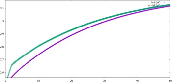
The solution of the eq. (1) can be illustrated by a numerical solution. In Figure 2, the LHS model on the left, represents actual US and EU carbon emissions and their growth rate decline. The RHS, model on the right, presents results of the simulations of the dynamic eq. (1), that includes a time-varying drift term through time-dependent growth rates.

Figure 2.

LHS: the actual decline of net emissions for the US and EU; RHS: non-stationary carbon emissions simulated; starting from the upper curve: $g_{ce}=0.002,$ $g_{ce}=0.0015$ , $g_{ce}=0.001$ , $g_{ce}=0.0005,$ and $g_{ce}=0.0001$ . Note: the lowest growth rate is not only flattening the curve, but reversing it.

In Figure 2, the parameters, $\alpha, $ $g_{ce}$ , and the variable $t$ will determine the shapes of the curves. In the Figure 2 LHS, the effects of an energy transition policy in creating a low carbon economy with a lower growth rate of emissions, $g_{ce}$ (or other forces generating lower GDP growth rates), can flatten or reverse the stock of carbon emission curves.

The five cases in Figure 2 RHS, read from above, represent declining growth rates of $g_{ce}$ , given by the lower envelope. The public policy measures—such as carbon tax, cap & trade, emission standards, new green technology for energy production—but also business cycle downturns with negative economic growth rates, bring down the emissions growth rates. This stylized fact seems to match the LHS graph.

RHS, in Figure 2 gives similar results: at each curve and at a later point, the growth rate of carbon emission shrinks. In fact, in the RHS, we have assumed a lower growth rate of emission over time, $g_{ce}=0.002,$ $g_{ce}=0.0015$ , $g_{ce}=0.001$ , $g_{ce}=0.0005,$ and $g_{ce}=0.0001$ . The previous growth rate flattens the curve, but only the lowest growth rate of CO2 emission of $g_{ce}=0.0001$ will reverse the curve. Then, for the growth rate of $g_{ce}=0.0005$ , the dissipation of the CO2 from the atmosphere is not sufficient to eventually bring the curve back to its 2000 level.Footnote ¹⁰

In this context, net zero carbon emissions means that the first term of the carbon emission dynamics eq. (1) cancels out the second term. Hereby, a slight increase in carbon stocks is allowed, given the atmospheric dissipation of carbon represented by the first term in eq. (1). Yet, note that the stock of carbon has reached a level that indicates the world has already moved beyond the carbon budget. In order to reverse this, the first term has to be larger than the second term, see Edenhofer et al. (Reference Edenhofer, Kadner, von Stechow, Schwerhoff, Luderer, Edenhofer, Kadner, von Stechow, Schwerhoff and Luderer2014). Yet, this takes time and presumably we will observe delayed effects as obstacles for this requirement. From our dynamic of eq. (1), and the curves of Figure 2, RHS, it is obvious that the sooner the growth rate of emissions $g_{ce}$ is brought down, the more the actual emission curve, as shown in Figure 1 will be flattened or even reversed. For Europe, this mechanism for halting the emission flows is more clear (see Figure 2, LHS). For the US, emission flows decrease to less than half, since the year 2000. But one should note that even for the EU economies, it has further decreased since the 2008-9 Global Financial Crisis (GFC) and the 2020 Covid shock.

We have the following explanation of the issue of a temporary decline of net emission since 2000 in the US and Europe, as shown in Figure 2, LHS, There was an economic cyclical effect, but also an effect from mitigation policies. In Figure 2, RHS, we observe a similar effect using declining growth rates of carbon emissions. In fact, both pictures might be explained by the work of Cohen et al. (Reference Cohen, Jalles, Loungani and Marto2018, Reference Cohen, Jalle, Loungani and Pizzuto2022) who use Okun’s gap theory to show that carbon emissions are decoupling growth rates (and decreasing) since the 2000s which can be represented by those two effects. Here, the two effects are also captured by the two components of eq. (1). The net emission goes down when the new emission slows down due to mitigation policies and business cycle effects. Yet overall, if the constraint of the carbon budget can not be maintained, the resulting vulnerabilities might trigger, tipping points and, accelerate climate-related disasters—see Greiner et al. (Reference Greiner, Gruene, Semmler, Greiner, Gruene and Semmler2010).

Another important aspect, stressed by climate researchers, is that delays until actual mitigation policies are activated or effective are too long for reducing the global warming (and thus extreme weather events), see also Nyambuu and Semmler (Reference Nyambuu and Semmler2023, ch. 9 and 10). Next, in a more generic model we will study a mix of both stationary and non-stationary variables and delayed effects.

3.1.2 The generic dynamic model with non-stationary and stationary variables

In order to study the macro policies, we combine the cyclical and the secular drivers of carbon emissions into a generic extension of the NLQ model used in Chen et al. (Reference Chen, Semmler and Maurer2022). However, we also add a slow-moving externality, as a carbon emissions trend, to drive a climate target for the generic model. Thus, the CB sets the interest rates ( $i$ ) based on its policy targets and current levels of inflation ( $\pi$ ), output gap ( $y$ ), credit flows ( $l$ ), and carbon emissions $(m)$ , but also has several different tools in its monetary operations toolbox for climate considerations. As often mentioned, the CBs’ monetary operations can help, but other measures, such as technological innovation, carbon pricing, financial and macro policies are also needed to affect the emission trend.

We presume in a finite horizon decision model a quadratic objective function given by eq. (2).

(2) \begin{equation} Min_{i(.)}\int _{0}^{T}e^{-\rho t}[w_{\pi }(\pi (t)-\pi _{s})^{2}+w_{y}(y(t)-y_{s})^{2}+w_{l}(l(t)-l_{s})^{2}+w_{m}(m(t)-m_{s})^{2}+w_{i}i(t)^{2}]dt \end{equation}

The CB exogenously sets the policy targets given by $\pi _{s},_{\,\,}y_{s},_{\,\,}$ and $l_{s}$ . Eq. (2) assigns a quadratic penalty to each variable deviation from their target value, and defines weights for each target. The weights are given by $w_{\pi },_{\,\,}w_{y},_{\,\,}w_{l}$ , $w_{i}$ and $w_{m}$ .Footnote ¹¹ Furthermore, the objective function faces the constraints of the macro behavior of each variable. The state variables are represented by the following dynamic state equations:

(3) \begin{align} \dot {\pi }(t)=-\alpha _{1}\pi (t)+\alpha _{2}y(t), & \,\,with\,\,\pi (0)=\pi _{0} \end{align}

(4) \begin{align} \dot {y}(t)=-\beta _{1}y(t)-\beta _{2}(i(t)+\sigma (y(t))-\pi (t)-r) & \,\,with\,\,_{_{}}y(0)=y_{0} \end{align}

(5) \begin{align} \dot {l}(t)=\gamma _{1}l(t)+\gamma _{2}(y(t))-\gamma _{3}(i(t)+\sigma (y(t)))-\gamma _{4}\pi (t), & \,\,with\,\,_{_{}}l(0)=l_{0} \end{align}

(6) \begin{align} \dot {m}(t)=-\sigma _{1}(m(t)-m_{s})+\frac {\sigma _{2}(y(t)+d(t))}{g_{r}(s)(\sigma _{3}l(t)+\sigma _{4}d(t))+\sigma _{5}}, & \,\,with\,\,m(0)=m_{0}\\[6pt]\nonumber \end{align}

The inflation dynamics are represented by a Phillips Curve, as in eq. (3). The inflation dynamics depend on the inflation itself, and the output gap, with a negative relationship with inflation and a positive relationship with the output gap.

The output gap dynamics, eq. (4), is given by a type of IS curve. The dynamics depend on the output gap itself, and the real interest rate term: $(i(t)+\sigma (y(t))-\pi (t)-r)$ . The real interest rate term, as defined by Faulwasser et al. (Reference Faulwasser, Gross, Semmler and Loungani2020), is composed of the nominal interest rate, $i(t)$ (policy rate, the control variable), increased by the risk premium, $\sigma (y(t))$ , and decreased by inflation, and the natural (or neutral) interest rate, $r$ . The model´s control variable $i(t)$ is the interest rate, a conventional monetary policy tool that responds to the inflation rate and the output gap, as in a conventional Taylor Rule. Furthermore, the CB’s action also responds to the level of credit flows.

As in Faulwasser et al. (Reference Faulwasser, Gross, Semmler and Loungani2020), a credit flow $l(t)$ dynamic is added in eq. (5) where the credit flows have feedback effects, rresponding positively to the output gap, and negatively to the interest rate, to the risk premium $\sigma (y(t))$ , and to the inflation rate, since we are assuming real credit flows.

Another novelty in our set up is adding a climate trend dynamic variable, eq. (6), to the model to account for future climate disruptions. CBs are presumed to monitor this variable when deciding on monetary policy. This new variable of eq. (6) is added as a new state equation to the system where it is assumed that CBs are able to impact the share of green credit flows $g_{r}$ (s) towards a green transition, which will be defined as time or state dependent; we presume $0\leq g_{r}(s)\leq 1$ . The share of green credit flows is 0 when CBs avoid to have a climate policy and 1 if CB policy helps to replace fossil fuel investments with green investments. The monetary authorities are usually monitoring the credit flows because they have a significant impact on their objectives—the output gap, inflation rate, and financial stability, see Coenen et al. (Reference Coenen, Lozej and Priftis2024).

Note that usually macrodynamic decision problems are explored based on stationary variables, see Cai and Judd (Reference Cai and Judd2023), with fluctuations over the business cycle. Empirical literature shows that emission dynamics are highly correlated with output gap cycles following the “Okun’s Law,” as demonstrated by Cohen et al. (Reference Cohen, Jalles, Loungani and Marto2018, Reference Cohen, Jalle, Loungani and Pizzuto2022). However, climate model—such as the Nordhaus DICE model (Nordhaus, Reference Nordhaus2008)—rely on economic growth models and depend on the levels of GDP and capital stocks (with a trend which is often augmented by population growth). To introduce a climate model perspective in a dynamic macro model, an additional variable $d(t)$ , representing a carbon emission trend as a drift term, needs to be added to the output gap to model the emission dynamics—that might or might not be impacted by macro policies.Footnote ¹²

The output gap can be defined in log form as: $y(t)=log(Y_{a}(t))-log(Y_{p}(t))$ , where $Y_{a}$ is the actual output and $Y_{p}$ is the potential output, which is actually affecting the drift term, $d(t),$ in eq. (6). Negative externality effects, such as weather extremes and climate disasters can reduce the potential output,Footnote ¹³ but one can assume that overall there is still a net growth rate of potential output:

(7) \begin{align} d(t)=log(e^{(g_{n}t)}) \end{align}

In eq. (7), the $g_{n}$ is the net growth rate of the potential output,Footnote ¹⁴ starting with period $t$ =1 as the first time period, which leads to dynamics such as eq. (7).

In our model, the risk premium, $\sigma (y(t))$ depends on the output gap—as in Chen et al. (Reference Chen, Semmler and Maurer2022)—and can also be indirectly impacted by green credit flows. It is reasonable to assume that green credit flows carry lower risk in the long-run, due to lower carbon emissions. The risk premium itself is driven by a non-linear relationship between risk and the output gap based on a discontinuous function. It increases with a negative output gap, but can also be affected by QE and other policies undertaken by the CB.Footnote ¹⁵

As shown in eq. (8), a discontinuous function simulates this regime change. The risk premium is capped at $mu_{1}$ , but a QE policy is able to decrease this maximum level of risk exogenously. Hereby, we follow Chen et al. (Reference Chen, Semmler and Maurer2022) and assume $mu_{1}:=0.15$ , then we have:

(8) \begin{align} \sigma (y(t))=\begin{cases} mu_{1} & \text { if }y(t)\leq 0\\ 0 & \text {otherwise} \end{cases} \end{align}

Eq. (8) represents an essential non-linearity arising from the state-dependent risk premium.

The emission dynamics $m(t)$ of eq. (6) is driven by itself (first term and the second term), by the actual and trend output as part of the numerator of eq. (6)— $\sigma _{2}(y(t)+d(t))$ —and also by the carbon emission and the mitigation policy, both represented in the denominator, defined in eq. (9) below. Given the role of $g_{r}(s)$ , the emission dynamics are impacted by the denominator of eq. (6) where the credit flows and the output trend play an important role:

(9) \begin{align} g_{r}(s)(\sigma _{3}l(t)+\sigma _{4}d(t))+\sigma _{5} \end{align}

Hereby, the first term is zero when there is no green credit flow for supporting the mitigation policy, otherwise it is 1.Footnote ¹⁶ One should note that for a matter of simplification, we have assumed only two extreme cases.

The carbon emission dynamic in eq. (6) is formulated in a similar way as in eq. (1), but in eq. (6) the exogenously-driven (time-dependent) second part of eq. (1) increases with a higher output $(y(t)+d(t))$ , but can also be decreased with a higher credit mitigation policy effort, indicated by $g_{r}(s)(\sigma _{3}l(t)+\sigma _{4}d(t))$ . Thus, the exogenous time-dependent part of eq. (1) is now endogenized. Note that the increasing green credit flows, possibly a policy tool, given by $g_{r}(s)$ , decreases the carbon intensity of the output $(y(t)+d(t))$ . As in the Nordhaus DICE model (Nordhaus, Reference Nordhaus2008), mitigation policy can decrease emission intensities per unit of output and thus, emission growth.

We can also relate the credit flow and emission dynamics to the financial conditions in general and more specifically to the interest rate. By assuming that higher credit flows to green investments occur under low interest rates.Footnote ¹⁷ Using this idea, $g_{r}$ (s) is made state dependent. Instead of taking $g_{r}$ as a continuous function of the interest rate, we are taking it as a discrete, step wise function. In eq. (9), we propose $g_{r}(s)(\sigma _{3}l(t)+\sigma _{4}d(t))+\sigma _{5}$ whereby $g_{r}(s)$ depends on the state of the interest rate: $s$ exhibits a threshold with interest rates over, or below, that threshold.Footnote ¹⁸ This means that lower interest rates promote green investments while higher interest rates slow down green investments.Footnote ¹⁹ Note that lower interest rates are also often associated with declining risk premia, appearing as conducive to issuing public bonds for the decarbonization of the economy, see Braga et al. (Reference Braga, Semmler and Grass2021).

Note that if there is a relevant emission trend and green credit flows, as defined in eq. (6), this might affect other CB goals—inflation rates, the output gap, and financial stability—and this in turn affects the risk premia and policy goals, see Coenen et al. (2024).

Next, we study the model’s numerical solutions when CBs allow for climate considerations. This type of policy is represented by the carbon emission dynamics in eq. (6) by the parameter $g_{r}$ (s), which for illustrative reasons will be taken 1 or 0. As also shown in the CBs network publications, NGFS, there are other monetary and financial policy operations possible, which we will discuss below.

3.2 Numerical Solutions of the Generic Model

This Section studies the macroeconomic impact of a monetary and financial policy response in a recession when the CB also pursues a climate objective and uses green operational policy instruments. The CB direct targets are: $\pi _{s}=0$ , $y_{s}=0$ , $l_{s}=0$ , and we use an indirect target for $m_{s}$ , $m_{s}=3.0$ , with an initial conditionFootnote ²⁰ $m_{0}=2.5$ . First, we solve the model for the cases with no policy delay ( $d=0$ ) if the economy faces at the initial period: (i) a positive output gap, inflation, and slightly positive credit flows; and (ii) a negative output gap, a slightly positive inflation rate, and positive credit flows.

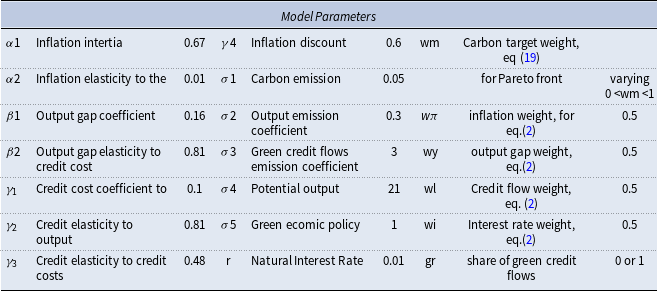
The following table, Table 1, contains the model parameters and values.

Table 1.

NLQ model parameters

The model versions presented in Section 3.1 are solved by using AMPL. A short sketch of the AMPL methodology with and without delays is presented in Appendices B and C.

Simulation 1

For the Simulation 1, the economy faces the following initial conditions: $\pi _{o}=0.015$ , $y_{o}=0.05$ , $l_{o}=0.05$ , $m_{o}=2.5$ . The CB keeps the interest rate high for a period of time, but decreases it to lower levels while the output gap and inflation decrease. This is why we take $g_{r}(s)$ as time or state dependent. In eq. (9) we have proposed $g_{r}(s)(\sigma _{3}l(t)+\sigma _{4}d(t))+\sigma _{5}$ whereby the $g_{r}(s)$ depends on time, or on the interest rate level. In the latter case, state $s$ exhibits a threshold with respect to the interest rates which will be higher above that threshold.

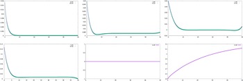
When the interest rates move down to 2%, we have a state of easy credit and the parameter $g_{r}(s)$ switches to 1. All interest rates above 2% will have a parameter $g_{r}(s)=0.$ The solutions to eqs. (3)–(5) turn out to be the same regardless of whether the state $g_{r}(s)$ is, 0 or 1, but the trajectories are different for the eq. (6). It depends on $g_{r}(s)$ , if it is 1 or $0$ . The trajectories for the state variables and the optimal interest rate are shown in Figure 3, below.

Figure 3.

Model simulation 1: above: inflation rate, positive output gap and credit flow; below: interest rate ( $u$ ), risk premium ( $sy$ ), and emission ( $m$ ) (when $g_{r}(s)=$ 0 or 1); emissions are controlled implicitly through $g_{r}(s)$ with time-dependent switches, as soon as interest rate moves down to 2%.

Note that, in Figure 3, the inflation rate, the output gap and the credit flows start positive and then rapidly move towards the zero-bound. The interest rate also starts at a high level and then rapidly decreases towards the zero-bound. CB monetary policy attempts to keep the inflation rate and the output under control. Given that the control $u(t)$ represents interest rate $i(t)=u(t))$ , the latter moves to the zero bound. The risk premium is zero at all times since the output gap never becomes negative. The emission moves steadily up and exhibits non-stationarity since there is a drift term in the eq. (6). The emissions arising from potential output is a driver for global warming. The dissipation of emissions can also be reduced, due to the first term of eq. (6). However, emissions from output, can drive global warming and climate disasters, becoming a peril in the long run and is studied further in Atolia et al. (Reference Atolia, Loungani, Maurer and Semmler2023).

3.2.1 Simulation 2

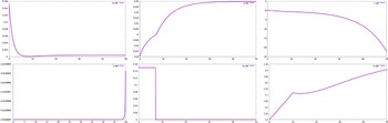
For the next simulation, see figure 4, we assume the economy faces the following initial conditions: $\pi _{o}=0.015$ , $y_{o}=-0.03$ , $l_{o}=0.05$ , $m_{o}=2.5$ and $m_{s}=3.0$ .

Figure 4.

Simulation 2: above: inflation rate, negative output gap, and credit flow; below: interest rate, risk premium and emission (when $g_{r}(s)=$ 0 up to period 10 then $g_{r}(s)=1$ ); time-dependent regime change and the risk premium stays high as long as the output gap is negative; the emission curve is first increasing then flattening when the credit flow for decarbonization is phased in.

The interesting overall observation in both cases, simulations 1 and 2, is that the dynamics of macro variables do not change much while green credit policy ( $g_{r}=1$ ) seems to significantly favor the decarbonization efforts as compared to a no green credit policy scenario ( $g_{r}=0$ ). As a green credit policy, we could have for example ECB’s TLTROs, as it has been generally engineered since 2014. Though in our set up we first worked with an exogenously given $g_{r}=1\thinspace \thinspace or\thinspace \thinspace 0,$ it is now utilized in a regime switching model when $g_{r}(s)=$ 0 up to period 10 then $g_{r}(s)=1$ , resulting in a flattening of the emissions curve. Here, the regime switch is modeled as a time-dependent regime change, whereby in the first 10 periods no acceleration of credit flows takes place for green credit flows. This issue will also be further explored below and in the econometric part of the paper, Section 4.

3.3 Numerical solution with delayed effects

Before exploring the econometrics of the model, we first introduce a model with delayed effects of policies. The technical features are discussed in Appendix C. The delay effects in these policies can come from decision delays and/or transmission delays. In the latter case, as the implementation of policies is supposed to work through transmission channels, their impact occurs slowly.Footnote ²¹ In fact, the growth rate of carbon emissions may slow down and reach net zero by 2030. Moreover, the stock of carbon emissions is projected to only start decreasing (slowly) after 2050, while weather extremes and climate disasters are still predicted to occur. Economists consider this a serious problem in climate economics research, see Nyambuu and Semmler (Reference Nyambuu and Semmler2023, ch. 9).

A dynamic finite horizon decision model with delayed effects is described by the following modified dynamics of eq. (6) while the remaining equations remain the same:

(10) \begin{align} \dot {m}(t)=g_{m_{0}}(t-d)-\sigma _{1}(m(t)-m_{s})+\frac {\sigma _{2}(y(t)+d(t))}{g_{r}(\sigma _{3}l(t)+\sigma _{4}d(t))+\sigma _{5}}, & \,\,with\,\,m(0)=m_{0} \end{align}

Eq. (10) replaces eq. (6). Eq. (10) now shows that the policy maker exerts her or his impact on the carbon emission variable with a decision delay and/or transmission delay.Footnote ²² This has effects on actual decarbonization. Thus, delay $d$ amounts to a sticky and still positive increase of $C02$ emissions, and a decarbonization delay of roughly 2 to 3 years.Footnote ²³ There is a positive growth of net emissions, $g_{m_{0}}(t-d),$ which is only after $d-$ periods slowly reduced through policies, while the natural decay of carbon, $-\sigma _{1}(m(t)-m_{s}),$ still occurs later when the emissions are controlled. The third term in eq. (10) is actually effective. In other words, the growth of emissions $g_{m_{0}}(t-d)$ continuous to increase until the emission reduction given by the denominator in the the third term of eq. (10) becomes effective.

The major difference between the previous set-up to the model with no delayed policy—which is arising in non-delayed controlled dynamic macroeconomics as compared to the delayed policy effects as in eq. (10)—is clearly observable in our numerical results for the stock of the $CO2$ emissions.

In the simulations, on the lower graph of Figure 5, when we assume a regime dependence of green investments and credit flows, the dynamics of carbon emissions depends on $g_{r}$ (s). In fact, in Figure 5 the emissions at the beginning rises faster with a delay and then slows down when the climate policies decision becomes effective through the third term of eq. (10). Here, the higher green credit flows are phased in after period 10 and the emissions $m(t)$ slow down since credit flows are eventually reducing the emissions to a lower level, once $g_{r}=1$ is phased in, generating improved credit flows for green investments. On the the other hand, high interest rates and worsening of financial conditions (rising risk premia and credit costs), are likely to slow down effective demand triggering a financially induced recession, which then reduces output growth causing carbon emissions to decline, see Cohen et al. (Reference Cohen, Jalles, Loungani and Marto2018, Reference Cohen, Jalle, Loungani and Pizzuto2022).

Figure 5.

Upper graph: model solution with delay, lower graph: no delay; both graphs with regime switching $g_{r}(s)$ of credit flows.

All together, the carbon budget is likely to move to its atmospheric constraints faster with policy and transmission delays than without those delays. Also, emissions accelerate with higher interest rates, higher risk premia, and with a lack of credit flows, as observable in the initial periods of the lower part of Figure 5. As to the delayed effects, as Nyambuu and Semmler (Reference Nyambuu and Semmler2023, ch. 10) discuss, there are many reasons why there might be delays in decisions, as well as in the transition mechanism of decarbonization policies. Reasons for delays include non-cooperative games in policy making, irreversibility of capital investments, and lock-ins in previous behavior, and policies.

Overall, the model outcomes of Sections 3.2 and 3.3 demonstrate the need for an active CB policy and support the view of including climate considerations in CBs policies. These climate facing CB policies are necessary because of the long-run negative externalities, generating upward trends in emissions with delayed impacts, that result from fossil fuel use by industrial and other sector’s activities. Yet, monetary policy and other CBs priorities—like inflation control, output gap, employment, and financial stability—can create constraints and make climate goals of CBs a great challenge.

But, as the CBs network NGFS argues, specific financial and monetary policy instruments and operations can be implemented to channel credit flows to green investments. There is of course still a need for other policies to support carbon emission reduction. Governments should, for example, promote green investments, complementary to the CBs efforts, with other types of climate policy, notably technology and fiscal policies.Footnote ²⁴ Furthermore, although recessions are reducing carbon emission, overall emissions are still rising.Footnote ²⁵ As we will show next, several types of policies and economic shocks are likely to affect the $C02$ emissions.

Table 2.

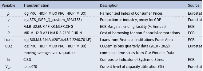
Data transformation and data sources

4. Empirical study— VECM with mixed stationary and non-stationary variables

In this Section, we address the econometric treatment of some of the issues discussed above, in particular how to deal with stationary and non-de-trended non-stationary variables. We use: “Industrial Output” and the “Harmonized Consumer Price Index” as measures of the real activity and the price level; “Current Level of Capacity Utilization” and “Composite Indicator of Systemic Stress,” as measures of the risk stress in the economy; “ECB Margin Lending Facility” as a direct monetary policy variable; “Cost of Borrowing for Non-financial Corporations” and “Loan from Financial Institutions,” as indirect policy variables. “CO2 Emissions Quarterly” is also used as the non-stationary variable, a critical variable for our investigation. The data sources and their transformation are summarized in Table 2.

Figure 6 presents a plot for the eight time series. Some of the time series data show considerable non-stationarity with co-movements across the time-series variables. However, other time series show features of stationary variables. VECM with co-integration relations are standard models for non-stationary time series because the stationary co-integrating relations among non-stationary data provide an appealing notion of equilibrium towards which the dynamic system is evolving. A large body of research works using VECM methodology can be found in the relevant literature.

Figure 6.

Plot of actual time series.

Applying a set of unit-root tests—ADF-test, KPSS-test and PP-test—to the eight time series we find that $p$ , $y$ , $r$ , $R$ , $Loan$ , and $CO2$ are I(1) series while $V_{c}$ and $fsi$ are I(0) series. A VECM seems to be a suitable econometric model for this set of data, but the standard VECM only applies to time series with the same degree of integration, i.e. if all time series are I(1). However in this case, there are two I(0) time series. Common practice is thus to exclude the I(0) variables from the co-integration analysis. We, however, want to keep the stationary variables in the model. Following the method in Gonzalo and Ng (Reference Gonzalo and Ng2001) and Chen et al. (Reference Chen, Semmler and Maurer2022), we use a constrained VECM to handle both mixed stationary and non-stationary variables.

To present the constraint, we start with a conventional VECM.

(11) \begin{align} \Delta Y_{t} = \alpha \beta ^{\prime} Y_{t-1} + \sum ^{L-1}_{j=1} \phi _j \Delta Y_{t-j} + u_{t} \end{align}

where $Y_{t}$ is an $n$ vector of variables, $\alpha$ and $\beta$ are $n\times h$ vectors of parameter with $h\lt n$ , and $u_{t}\sim i.i.d.N(0,\Omega )$ represent the noise. We also consider $h$ as the dimension of the co-integration space, i.e. the dimension of the I(0) space.

We decompose the variables into two subsets. Let $Y_{t}=(Y_{1t}^{\prime},Y_{2t}^{\prime})^{\prime}$ with $Y_{2t}$ is $k$ -dimensional I(0) series and $Y_{1t}$ is $n-k$ dimensional I(1) series. Decomposing the co-integration vectors accordingly we have:

(12) \begin{eqnarray} \left [\begin{array}{c} \Delta Y_{1,t}\\ \Delta Y_{2,t} \end{array}\right ] = \left [\begin{array}{c@{\quad}c} \beta ^\prime _{11} & \beta ^\prime _{12}\\ \beta ^\prime _{21} & \beta ^\prime _{22} \end{array}\right ] \left [\begin{array}{c}Y_{1,t-1}\\ Y_{2,t-1}\end{array} \right ] + \sum ^{L-1}_{j=1} \phi _j \Delta Y_{t-j} + u_t \end{eqnarray}

The necessary and sufficient condition for $Y_{t}$ to contain $k$ I(0) components are formulated as follows:

(13) \begin{equation} \mathcal {H}_{m}\,:\,\beta _{12}^{\prime}=0\mbox { and }\beta _{21}^{\prime}=0. \end{equation}

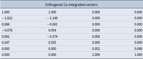
The constraints imply that the co-integration space, i.e. the I(0) space, of a mixed VECM can be decomposed into two orthogonal sub-spaces: the I(0) subspace spanning the I(0) variable, and the I(0) subspace of the linear combinations of the I(1) variables. These two restrictions are intuitively appealing. Indeed, $\beta _{12}=0$ and $\beta _{21}=0$ as I(1) variables do not form linear combinations with I(0) variables to become stationary.

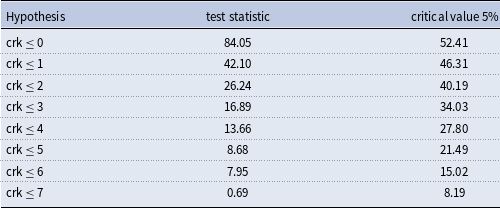
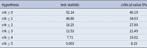
Condition (13) implies that a mixed VECM with I(1) and I(0) components is a special case of a conventional VECM, with restrictions on the co-integrating vectors. Therefore, the Johansen procedure can be used to determine the co-integration rank—i.e. the dimension of the I(0) space—and a test of the presence of I(0) components can be conducted with the condition (13) as the null hypothesis. It is worth noting that the Johansen’s test gives the dimension of the I(0) space, but not the number of independent co-integration relations in a mixed VECM. In a VECM where all variable are I(1), the dimension of the I(0) space corresponds to the number of independent co-integration relations. In a mixed VECM with six I(1) variables and two I(0) variables, if the Johansen’s test results in $rank=4$ , this implies that there are two I(0) components, and two independent co-integration relations among the six I(1) variables.

Both conditions are linear restrictions on $\beta$ . Following Boswijk and Doornik (Reference Boswijk and Doornik2004), linear restrictions on $\alpha$ and $\beta$ can be formulated in the following form:

(14) \begin{equation} \mbox {vec}(\alpha ^{\prime})=G\psi,\quad\mbox {vec}\beta =H\phi +h_{0}, \end{equation}

where $G$ and $H$ serve as selection matrices and $\psi$ and $\phi$ are freely varying parameters. If there are no restrictions on $\alpha$ , $G$ is chosen as an identity matrix, and hence $\mbox {vec}(\alpha ^{\prime})=\psi, $ and all elements of $\alpha$ are freely varying parameters. Similarly, $H$ is also a selection matrix. $H$ is chosen as an identity matrix and $h_{0}={\bf 0}$ . If there are no restrictions on $\beta$ and if the $i-th$ element of $\mbox {vec}\beta$ is restricted to be zero, $H$ is obtained by leaving out the $i-th$ column of the identity matrix and the $i-th$ element of $h_{0}$ is set to be $0$ . If the $i-th$ element of $\mbox {vec}\beta$ is a constant $c$ , $H$ is obtained by leaving out the $i-th$ column of the identity matrix and the $i-th$ element of $h_{0}$ is set to be $c$ .

Boswijk and Doornik (Reference Boswijk and Doornik2004) propose the following iteration process to calculate the constrained parameter and thus to test the hypothesis related to the constraints.

\begin{equation*} \tilde {\psi }(\phi, \Omega )=[G^{\prime}(\Omega ^{-1}\otimes \beta^{\prime}S_{11}\beta )G]^{-1}(\Omega ^{-1}\otimes \beta^{\prime}S_{11})\mbox {vec}(\hat {\Pi }^{\prime}_{LS}) \end{equation*}

\begin{equation*} \tilde {\phi }(\psi, \Omega )=[H^{\prime}(\alpha ^{\prime}\Omega ^{-1}\alpha \otimes S_{11}\beta )H]^{-1}H^{\prime}(\alpha ^{\prime}\Omega ^{-1}\otimes S_{11})\Big [\mbox {vec}\big (\hat {\Pi }^{\prime}_{LS}\big )-(\alpha \otimes I_{p1})h_{0}\Big ]. \end{equation*}

\begin{equation*} \tilde {\Omega }(\psi, \phi )=S_{00}-S_{01}\beta \alpha ^{\prime}-\alpha \beta ^{\prime}S_{10}+\alpha \beta ^{\prime}S_{11}\beta \alpha ^{\prime}, \end{equation*}

where $\Omega$ is the covariance matrix of the residuals $u_{t}$ in VECM in (11), $S_{01}$ , $S_{11}$ , and $S_{00}$ are the cross products of the two auxiliary regressions in the Johansen procedure.

(15) \begin{equation} S_{00}=\frac {1}{T}(\Delta Y^{\prime}\Delta Y-\Delta Y^{\prime}W[W^{\prime}W]^{-1}W^{\prime}\Delta Y), \end{equation}

(16) \begin{equation} S_{11}=\frac {1}{T}(Y_{-1}^{\prime}Y_{-1}-Y_{-1}^{\prime}W[W^{\prime}W]^{-1}W^{\prime}Y_{-1}), \end{equation}

(17) \begin{equation} S_{01}=S^{\prime}_{10}=\frac {1}{T}(\Delta Y^{\prime}Y_{-1}-\Delta Y^{\prime}W[W^{\prime}W]^{-1}W^{\prime}Y_{-1}), \end{equation}

where the $\Delta Y$ , $Y_{-1}$ and $W$ are the data matrices (consisting of $T$ rows) of $\Delta Y^{\prime}_{t}$ , $Y^{\prime}_{t-1}$ and $W^{\prime}_{t}$ with $W^{\prime}_{t}=\Delta Y^{\prime}_{t-1},\ldots, \Delta Y^{\prime}_{t-p}$ , and $\hat {\Pi }_{LS}=S_{01}^{-1}S_{11}^{-1}$ .

Starting from a set of initial values $(\psi _{0},\phi _{0},\Omega _{0})$ , the iterations then become ${\psi }_{j}=\tilde {\psi }(\phi _{j-1},\Omega _{j-1})$ , ${\phi }_{j}=\tilde {\phi }(\psi _{j},\Omega _{j-1})$ , ${\Omega }_{j}=\tilde {\Omega }(\psi _{j},\phi _{j})$ . The iteration procedure stops when the changes in estimated values between two steps are below a prescribed threshold. According to Boswijk and Doornik (Reference Boswijk and Doornik2004), the following likelihood ratio is asymptotically $\chi ^{2}$ with degree of freedom $rk$

(18) \begin{equation} \mathcal {LR}(\mathcal {H}_{m}|\mathcal {H}_{u})=T\big [\log |{\tilde {\Omega }}|-\log |\hat {{\Omega }}|\big ] \xrightarrow{d} \chi ^{2}(rk), \end{equation}

where $\tilde {\Omega }$ is the constrained estimate under constraint (13) and $\hat {\Omega }$ is the unconstrained estimate in (12) denoted by $\mathcal {H}_{u}$ .

This likelihood ratio test can be used to test the number of I(0) variables in a mixed VECM. For the hypotheses of 1, 2, 3, I(0) components $b_{12}$ and $b_{21}^{\prime}$ are ( $7\times 1$ ), ( $6\times 2$ ) and ( $5\times 3$ ) matrices of zeros respectively. The p-values of the three tests are: 0.31, 0.048, and 0.01 respectively. We conclude that there are two I(0) variables and that the p-value is slightly less than 0.05.

For the estimated mixed VECM, we calculate the impulse response functions. To avoid the problem of identification of shocks, we use the generalized impulse response proposed in Pesaran and Shin (Reference Pesaran and Shin1998). The shocks are all one-unit positive shocks.

In the subsequent figures, we have summarized the shocks to both non-stationary and stationary variables and their effect on the CO2 emissions. Details of the Impulse Response trajectories from any of the eight variables to other variable are reported in Appendix D.

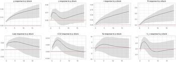
The econometric analysis, with mixed stationary and non-stationary variables, predict shocks to non-stationary variables and show a mean reversion to the stationary variables. In Figure 7, we report only the IRs of the shocks of each macro variable on the CO2 emissions and observe some important results.

Figure 7.

CO2 responses, impulse responses.

First, as Figure 7 shows, a shock to a non-stationary variable, such as GDP, is correlated with the growth rate shift of CO2 emissions. Their growth rates depend heavily on the GDP shocks and experiences which shifts with higher GDP. At the beginning there is some overshooting of the CO2 emissions with a subsequent reduction. But overall there is an upward shift. Since the price level is correlated with the GDP growth, a similar effect can be seen for the impact of the price level shocks on CO2 emissions, though less pronounced. Conversely, if the GDP shock is negative, it would lead, at least in the shorter-run, to a decline of CO2 emissions, see also Cohen et al. (Reference Cohen, Jalles, Loungani and Marto2018, Reference Cohen, Jalle, Loungani and Pizzuto2022).Footnote ²⁶

Second, a further result of Figure 7 is that shocks to other non-stationary variables, such as financial condition (credit cost), cause level shifts: a rise of the interest rate and the risk premium will reduce the CO2 emissions. This is likely the effects of the rising cost of borrowing and output contractions. These are also macroeconomic demand effects: falling demand and output contraction will reduce CO2 emissions. There is also a supply effect: positive credit or loan shocks, and an increase in credit flows, as we have found in Figure 6, is likely to decrease emissions in the longer run (see the non-stationary effect of a loan shock in Figure 7). Higher credit flows, possibly accompanied by a lower cost of borrowing, are likely to cause more green investments and lower CO2 emissions.Footnote ²⁷

Third, in Figure 7, for the stationary variables, a shock to the Financial Stress Index (FSI) leads to a decline in CO2 emissions, presumably through more financial stress and output decline. In contrast, for rising capacity utilization, a temporary rise in the CO2 emission occurs. These are also two plausible results. In the latter two cases we can, however, as predicted, observe mean reversion to zero, since both variables are constructed as stationary.

As to operational tools of CBs, one can classify interest rates, credit cost, and credit flows as direct operational tools against climate risks, but the output variation only as an indirect tool (which, of course, CBs cannot steer easily). Moreover, we can observe, see eqs. (3)–(6) and Appendix D, that each possible operational tool of CBs to reduce CO2 emissions and avoid climate risk has side effects on other targets and objectives.

As Allen et al. (Reference Allen, Mathieu Boullot, D?es, de Gaye, Lisack, Thubin and Wegner2023) argue, macroeconomic imbalances and disruptions are likely to be present through dynamically generated imbalances resulting from climate risks and/or transition efforts to a low carbon economy. CBs are thus not neutral given their target imbalances. It thus raises the question of what relative weights should CBs assign to their policy objectives (and goals), so they can manage multiple vulnerabilities when their objectives have become imbalanced.

5. How to manage multiple vulnerabilities and conflicting goals?

Whereas the above solutions in Section 3 assume fixed and equal weights for the multiple targets, CBs are usually confronted with multiple vulnerabilities and conflicting goals arising at certain time periods. CBs have to manage, and need to set, primary objectives for a certain time period. Often CBs confirm that they have multiple worries, but are optimistic by stating that they have tools and operational instruments for the different objectives. But as Allen et al. (Reference Allen, Mathieu Boullot, D?es, de Gaye, Lisack, Thubin and Wegner2023) argue, climate risk will generate threats to the other macroeconomic targets as well.

In this spirit, we introduce a method that helps prioritizing objectives and their time variation. We explore what the suitable weights for certain objectives could be to manage these multiple goals. We also briefly discuss time varying objectives for different time horizons, indicated by a regime-switching model, see also Brunnermeier and Landau (Reference Brunnermeier and Landau2021).

The managing of multiple vulnerabilities and conflicting goals with the prioritizing policy decision objectives when several macroeconomic worries have emerged is indeed an important issue of dynamic decision making, where one has to assign plausible weights to the objectives. We are motivated by Kaya and Maurer (Reference Kaya and Maurer2023) who revive a traditional construction known as Pareto front. We transform our dynamic decision problem with multiple objectives into a bi-objective problem.Footnote ²⁸ We want to note that such an exploration is particularly needed when multiple vulnerabilities and conflicting goals interact—and which could be quite disruptive.

We include the monitoring of the squared deviation of actual emission from a target emission $(m(t)-m_{s})^{2}$ in the multiple objective function.Footnote ²⁹ We then decompose the problem of decision making with multiple objectives into two sub-problems by assigning different weights to the sub-problems to obtain a final solution. Let us define a sub-divided function with two groups of objectives where we also include the trend of the carbon emissions:

(19) \begin{equation} Min_{i(.)}\int _{0}^{T}e^{-\rho t}[w\{(\pi (t)-\pi _{s})^{2}+(y(t)-y_{s})^{2}+(l(t)-l_{s})^{2}\}+(1-w)\{(m(t)-m_{s})^{2}+i(t)^{2}\}]dt \end{equation}

Hereby, one sub-group of objectives has the weight $w$ and the other the weight $(1-w)$ whereby we introduce a loop of a varying $w,$ with $0\leq w\leq 1$ , to the two following sub-integrals that are computed recursively, but are connected in a loop with eq. (19). The two looped sub-integrals are:

(20) \begin{equation} int1=\int _{0}^{T}e^{-\rho t}[\{(\pi (t)-\pi _{s})^{2}+(y(t)-y_{s})^{2}+(l(t)-l_{s})^{2}\}]dt \end{equation}

and

(21) \begin{equation} int2=\int _{0}^{T}e^{-\rho t}[\{(m(t)-m_{s})^{2}+i(t)^{2}\}]dt \end{equation}

Note that other bi-objective problems could be chosen as well.

Here, we have chosen the above two bi-objective, denoting two groups of objectives used to solve the integral eq. (19), but one sub-group is relevant for the climate considerations of the policy makers. Then the aggregate integral value should have a minimum at $0\leq w\leq 1$ .Footnote ³⁰ Given our dynamic state equations of eqs. (3)–(6) and the recursively solved eqs. (19)–(21) with varying weights $w$ , we obtain the following Pareto front, resulting from a global minimum of eqs. (19)–(21) when the weight $w$ varies.

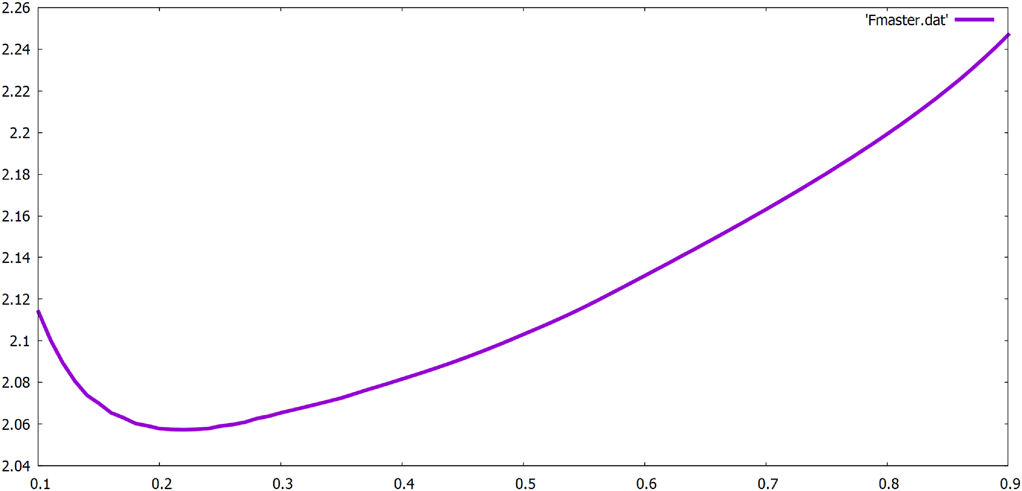
The Fmaster functionFootnote ³¹ of Figure 8 is based on eqs. (19)–(21), using the above initial conditionsFootnote ³² and the loops for $w$ , which provide at the global minimum of the Fmaster function, proper weights for prioritization of objectives for the decision maker considering multiple macroeconomic worries.Footnote ³³ The solution of the Fmaster function which represents a Pareto front provides the suitable weights for the first and second objective functions when those are viewed as desirable objective groups. In the above case, the weights should be roughly $w=0.2$ and $(1-w)=0.8$ , at the minimum of the curve in Figure 8.

Figure 8.

Fmaster function for the pareto front, with initial conditions and parameters: $m_{0}=2.5$ and $m_{s}=3.0$ for eqs. (19)–(21) and $\pi _{o}=0.015$ , $y_{o}=0.05$ , $l_{o}=0.1$ ;  $m_{0}$ corresponds to the current situation and $m_{s}$ to the requirement to keep the carbon emission below the constraints of the carbon budget.

Furthermore, Brunnermeier and Landau (Reference Brunnermeier and Landau2021) raise an important issue concerning the time horizon for different objectives. They state that central banks have shorter, business cycle oriented objectives, such as inflation, output and financial stabilization; and longer run objectives, for example climate goal oriented objectives. This issue could also be treated in this context by using a dynamic model with different decision horizon, as proposed by a number of papers in Haunschmied et al. (Reference Haunschmied, Kovacevic, Semmler and Veliov2020), and see also Di Bartolomeo et al. (Reference Di Bartolomeo, Minooei Fard and Semmler2023), where there is a model with a shorter run and longer run decision making process. A further discussion of measures against climate risks and operational tools of CBs is relegated to appendix E.