1. INTRODUCTION
High-power and high-energy lasers have increasingly wide applications in many fields, such as inertial confinement fusion (Moses, Reference Moses2009; Edwards & Danson, Reference Edwards and Danson2015; Obenschain et al., Reference Obenschain, Lehmberg, Kehne, Hegeler, Wolford, Sethian, Weaver and Karasik2015), industrial processing (Beck et al., Reference Beck, Parry, MacPherson, Waddie, Weston, Shephard and Hand2010), optoelectronic countermeasures (Elder, Reference Elder2010), and scientific research (Remo & Adams, Reference Remo and Adams2008; Divoky et al., Reference Divoky, Smrz, Chyla, Sikocinski, Severova, Novak, Huynh, Nagisetty, Miura and Pilař2014; Bai et al., Reference Bai, Wang, Lu, Yuan, Zheng, Li, Chen, Liu, Cui, Wang and Liu2016b ; Yu et al., Reference Yu, Hu, An, Qian, Wu, Zhang, Gu, Wang and Zheng2016). In particular, requirements of the good near-field beam quality in many research areas are more demanding than ever. However, long-path propagation of the beam and the increased number of optics elements will reduce the near-field beam quality in high-power laser systems. The output near-field modulation of the beam after propagation is mainly caused by the diffraction effect which is related to the initial input phase distribution (i.e. wavefront) of laser beam. According to Fresnel diffraction theory, the relation between final electric intensity distribution and initial electric intensity distribution (including phase and intensity) can be observed easily (Teich & Saleh, Reference Teich and Saleh1991). To date, description of the various ways of modeling laser beam propagation have been reported somewhere. For example, in 2003, O. Morice from CEA, France developed Miro to perform propagation computation to calculate how the spatial and temporal profiles will be transformed when passing through the components of the chain by using some propagation models including the Fresnel diffraction mode, the paraxial non-linear Schrodinger approximation and broadband mode (Morice, Reference Morice2003; Mainguy et al., Reference Mainguy, Tovena-Pecault and Le Garrec2005). In 2007, C. Dorrer from the University of Rochester used the transport-of-intensity equation to link the intensity and phase of an optical source and to describe the influence of characterization of high-frequency surface modulation based on Fresnel diffraction mode (Dorrer & Zuegel, Reference Dorrer and Zuegel2007a ,Reference Dorrer and Zuegel b ). Quite a part of works mainly concerned including linear propagation of the beam in high-power lasers (Simmons et al., Reference Simmons, Hunt and Warren1981), beam propagation in non-linear media (Chen et al., Reference Chen, Li, Chen, Pu, Zhang and Zhu2013; Semak & Shneider, Reference Semak and Shneider2015), flattened Gaussian beam propagation in free space (Lu & Luo, Reference Lu and Luo2000; Grant & Abdolvand, Reference Grant and Abdolvand2014), flat-topped beam propagation in turbulent media (Eyyuboğlu et al., Reference Eyyuboğlu, Arpali and Baykal2006), the influence of optical elements on the output laser beam profile in propagation (Wilfert et al., Reference Wilfert, Komrska, Poliak and Kolka2011), and the inter-related physical mechanisms in the processes of atmospheric propagation and lasing (Sprangle & Hafizi, Reference Sprangle and Hafizi2014). However, no detailed explanation and subsequent studies were reported which focus on the effects of the initial wavefront distortion on the output near-field characteristics in propagation of the flat-topped beam.
In fact, the wavefront distribution can be described according to the spatial frequency and it is decomposed as low-frequency term and high-frequency term. Both the low- and high-frequency phase distortion of the input has influence on the output near field. So it is important to clarify the different influence of wavefront distortion and the relevant physical mechanism. This is our focus and contribution in this paper. In this work, the mechanism of how the input wavefront distribution affects the output near-field beam quality are studied in detail by numerical simulation by using the fast Fourier transform method from the Helmholtz equation. The influence of low- and high-frequency wavefront aberrations on the output near-field modulation and fluence contrast is analyzed.
2. METHODS
In the simulation, the laser beam is assumed as to be a round size with super-Gaussian distribution. Considering the spatial symmetry of the laser beam, only the variations of the physical quantities in the x direction has been taken into account in the simulation. Using the slowly varying amplitude approximation and ignoring the temporal influence, the amplitude of the electric field of the laser can be expressed as:
 $$E(x) = A_0\exp \left[ { - {\left( {\displaystyle{x \over d}} \right)}^n} \right]\exp \left[ {i{\rm \varphi} _0(x)} \right]$$
where A 0 is the amplitude, the maximum value of the function; d is beam radius; φ0(x) is transverse initial phase of laser beam; n is the order of spatial super-Gaussian distribution, related to the rapidity of the transition from the maximum value to zero. For n = 2, a super-Gaussian reduces to a Gaussian function, whereas the higher the n, the flatter the profile is. In the limit n→∞, it tends to the function rect(x/2d).
In the laser system, because the thermal effects and the non-uniform amplification contributes to the existence of the transverse spatial phase distortions, φ0(x) is not constant anymore. In a high-power laser, there are several factors affecting the wavefront distortion in the laser system (Williams et al., Reference Williams, Auerbach, Henesian, Lawson, Hunt, Sacks and Widmayer1998), including the surface distortion of the reflecting mirror; wavefront distortion caused by the transmission through optical elements such as polarizer and window; pumped dynamic thermal distortion and residual heat; the spherical aberration and eccentric coma; and air turbulence. The phase of the laser will be modulated and distorted as it passes through the optical components in the laser system, the distorted phase φ0(x) is named as an additional phase with a random distribution and can be expressed as (Williams et al., Reference Williams, Auerbach, Hunt, Lawson, Manes, Orth, Sacks, Trenholme and Wegner1997; Fu & Zhang, Reference Fu and Zhang2012; Fan et al., Reference Fan, Lu, Lin, Yang, Liu, Dong, Zhu and Hasi2013):
 $${\rm \varphi} _0(x) = {\rm \varphi} _{0{\rm L}}(x) + {\rm \varphi} _{0{\rm H}}(x)$$
where φ0L(x) and φ0H(x) represent the low- and the high-frequency additional phases, respectively. According to the Power Spectral Density proposed as primary specifications in National Ignition Facility (NIF) teams, the low-frequency phase features with long scale lengths larger than 30 mm and the high-frequency phase is smaller which is about 30–0 mm; but the exact ranges and values for these specifications have not been fully determined at this point (Williams et al., Reference Williams, Auerbach, Hunt, Lawson, Manes, Orth, Sacks, Trenholme and Wegner1997). The corresponding formulas are given by:
 $${\rm \varphi} _{0{\rm L}}(x) = A \cdot {\rm Random}\,{\rm (}\! -\! 1,\,1{\rm )} \otimes \exp \left[ { - {\left( {\displaystyle{x \over {S_{{\rm gx}}}}} \right)}^2} \right]$$
 $${\rm \varphi} _{0{\rm H}}(x) = {\rm \sigma} \cdot {\rm Random} \,( - 1,\,1{\rm )}$$
Here, The low-frequency φ0L(x) follows a random Gaussian distribution, generated by convolving a Gaussian function with a uniformly distributed random number sequence. In Eq. (3), A is the amplitude coefficient and S gx is the factor determining the size of the phase distortion along the x-axis. The high-frequency φ0H(x) is a uniformly random distribution, where σ is the disturbing amplitude. The random numbers in Eqs (3) and (4) are generated from the computer.
Affected by diffraction effects of the long-path beam propagation in free space, due to spatial phase distortion, the spatial intensity distribution will be modulated. In free space, the laser beam propagation can be expressed according to Helmohtz equations as following:
 $$\nabla ^2E(x,\,t) - \displaystyle{{n_0^2} \over {c^2}} \,\,\displaystyle{{\partial ^2} \over {\partial t^2}}E(x,\,t) = 0$$
Within the framework of paraxial approximation, the solution of Eq. (5) can be written as the form of scalar Huygens–Fresnel integral as following:
 $$E(x) = \displaystyle{1 \over {{\rm i\lambda} z}}\exp \left( {{\rm i}kz} \right)\int\limits_{ - \infty} ^{ + \infty} {E_0(x_0)\exp \left[ {\displaystyle{{{\rm i\pi}} \over {{\rm \lambda} z}}{(x - x_0)}^2} \right]dx_0} $$
where λ is the wavelength of laser beam, z is the transmission distance, E 0(x 0) and E(x) are electrical field distribution of input and output laser beams.
In the high-power laser system, the laser peak intensity should be limited and the output laser near-field uniformity should be improved; otherwise, many unwanted non-linear optical effects such as self-focusing and stimulated light scattering will occur, which lead to laser energy losses and even optical element damage (Bahk et al., Reference Bahk, Zuegel, Fienup, Widmayer and Heebner2008; Hongjie et al., Reference Hongjie, Jin, Fengrui, Xinda, Xin, Xiaoyan, Laixi, Xiaodong, Zhan and Wanguo2013; Liao et al., Reference Liao, Raymond, Gaylord, Fallejo, Bude and Wegner2014). Therefore, it is necessary to study how the wavefront distortion affects the spatial laser intensity in the near field to provide a reference for a better design of the laser system. Fluence modulation value is one of the key parameters describing the characteristics of a laser beam in the near field, and it is expressed as (Runkel et al., Reference Runkel, Hawley-Fedder, Widmayer, Williams, Weinzapfel and Roberts2005; Li et al., Reference Li, Wang, Lu, Ding, Du, Chen, Zheng, Ba, Dong and Yuan2015):
 $$M_{\rm F} = \displaystyle{{F_{\max}} \over {F_{{\rm avg}}}}$$
where F max and F avg are the peak fluence and average fluence of the near-field distribution. In general, the smaller the value of M F is, the more uniform the near field is. In a high-power laser system, the near-field beam photographs is the relative intensity obtained by computer reduction of densitometer scans of the photographs. The peak-to-average intensity modulation in the photograph is the fluence modulation (Speck et al., Reference Speck, Bliss, Glaze, Herris, Holloway, Hunt, Johnson, Kuizenga, Ozarski and Patton1981).
The fluence contrast is also used to describe the near-field beam quality universally in high-power laser systems. High-power operation of laser systems was limited by small-scale beam breakup (Manes & Simmons, Reference Manes and Simmons1985; Van Wonterghem et al., Reference Van Wonterghem, Murray, Campbell, Speck, Barker, Smith, Browning and Behrendt1997), driven by the non-linear index of the transmission optics elements in the beam path. Small-scale contaminants or optics imperfections on the surface of the optics elements will lead to beam intensity modulations. At high intensity of the laser, these modulations are amplified and focused by the non-linear index effect. An early sign of the development of this instability is growth in the beam contrast, defined as the standard deviation of the fluence divided by its mean value. Contrast is measured by taking a sample of the near-field beam, projecting it on a camera, and calculating the fluence variation as recorded in the near-field camera image (Haynam et al., Reference Haynam, Wegner, Auerbach, Bowers, Dixit, Erbert, Heestand, Henesian, Hermann and Jancaitis2007). Fluence contrast can be defined as:
 $$C = \displaystyle{1 \over {F_{{\rm avg}}}}\displaystyle{{\int\!\!\int_s {{(F(x,\,y) - F_{{\rm avg}})}^2dxdy}} \over S}$$
where F(x,y) is the near-field fluence distribution and S is the beam area.
3. RESULTS AND DISCUSSION
When the laser beam propagates in free space, the near-field distribution is related to the transmission distance L, the beam aperture D and the laser wavelength λ, namely laser near-field changes with the Fresnel number of the beam. Fresnel number is defined as:
 $$F = \displaystyle{{D^2} \over {{\rm \lambda} L}}$$
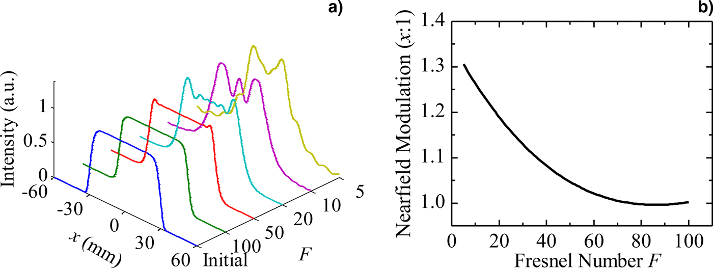
In the simulation, we assume that the laser beam is 14-order super-Gaussian in spatial distribution with the beam diameter of D = 60 mm and the laser wavelength of λ = 1053 nm. Firstly, to study the relationship between the output near field and the Fresnel number, the initial laser wavefront distribution is assumed to be flat-topped [i.e. φ0(x) = 0]. According to the beam propagation theory introduced above, the simulation results of the near-field intensity distribution of input laser and output laser at the Fresnel number from 5 to 100 is shown in Figure 1(a). When the beam size and the wavelength is set, different Fresnel number means different transmission distance. As shown in Figure 1(a), it suggests that the output near field is nearly flat-top when Fresnel number F = 100 and 50. On the other hand, the modulation appears in the near field when F < 50, such as F = 20, 10, and 5. As shown in Figure 1(b), when Fresnel number is 5, the output near-field modulation is about 1.3:1. The near-field modulation M F decreases with the increase of Fresnel number F in the whole trend. When the Fresnel number is larger than 50, the output near-field modulation is close to be 1. It can be concluded that F should be larger than 50 for getting a high-quality near field in propagation for the initial flat-topped laser beam.
The near field in propagation versus the Fresnel number. (a) Near-field intensity distribution of initial laser and output laser with different Fresnel number; (b) near-field modulation M F against Fresnel number.

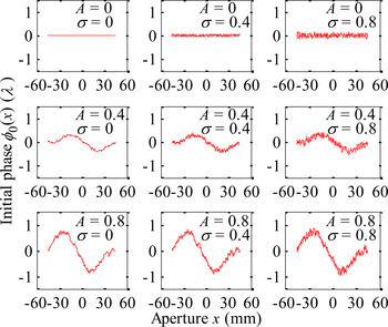
In the numerical simulation, the beam diameter is set to be D = 60 mm and the parameter of high-frequency phase distribution φ0H(x) is set to be S gx = 30 mm. A and σ of the additional phase distribution φ0(x) are not invariable. The distribution of initial wavefront distortion in the calculation is generated randomly, as shown in Figure 2. The range of the low- and high-frequency phase coefficient is from 0 to 1. The whole wavefront shape is related to both low-frequency phase coefficient A and high-frequency phase coefficient σ. When A and σ are small, the wavefront distortion is small. Wavefront distortion increases with the increase of A or σ. The wavefront is flat-topped under the special condition when both A and σ are 0 at the same time.
The initial wavefront distortion.

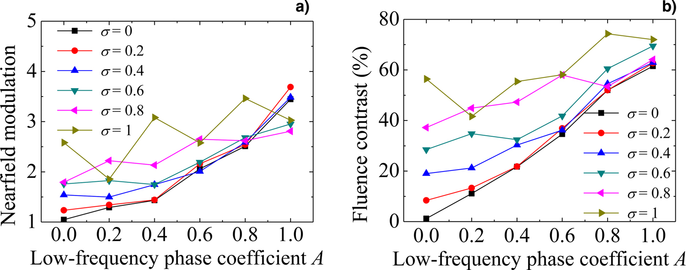
In the next step, the influence of A and σ on the output near field will be studied. In the following numerical simulations, the Fresnel number is set to be 50. The relation between low-frequency wavefront distortion and near-field modulation and fluence contrast is shown in Figure 3. Near-field modulation and fluence contrast increase with low-frequency phase coefficient A, and the trend intensifies when high-frequency phase coefficient is small, such as σ < 0.6. In general, the output fluence contrast should be controlled at the level of <30% and near-field modulation should be <2 for many applications of the high-power lasers (Bai et al., Reference Bai, Zhang, Liao, Zhou, Zhang, Chen, Ye, Jiang, Wang, Luan, Yuan and Zheng2016a ). In fact, the output near-field modulation is <2:1 (some even to 1.3:1) in many large high-power laser systems, such as NIF in Lawrence Livermore National Lab (LLNL) in the USA (Van Wonterghem et al., Reference Van Wonterghem, Burkhart, Haynam, Manes, Marshall, Murray, Spaeth, Speck, Sutton and Wegner2004), OMEGA EP Laser Facility in the University of Rochester (Barczys et al., Reference Barczys, Bahk, Spilatro, Coppenbarger, Hill, Hinterman, Kidder, Puth, Touris and Zuegel2013), the SG-III Laser Facility in China (Zhang et al., Reference Zhang, Zheng, Wei, Jing, Sui, Zheng, Xu, Yuan, Jiang and Yang2008), the HiLASE system in development in Institute of Physics ASCR in Czech Republic (Divoky et al., Reference Divoky, Sikocinski, Pilar, Lucianetti, Sawicka, Slezak and Mocek2013; Pilar et al., Reference Pilar, Slezak, Sikocinski, Divoky, Sawicka, Bonora, Lucianetti, Mocek and Jelinkova2014), the HELEN system at the Atomic Weapons Establishment (AWE) in the UK (Norman et al., Reference Norman, Andrew, Bett, Clifford, England, Hopps, Parker, Porter and Stevenson2002), the Optical Sciences Laser (OSL) in LLNL (Nostrand et al., Reference Nostrand, Weiland, Luthi, Vickers, Sell, Stanley, Honig, Auerbach, Hackel and Wegner2004), and the Hundred-Joule-level, nanosecond-pulse Nd:glass laser system in the Harbin Institute of Technology (Li et al., Reference Li, Wang, Lu, Ding, Du, Chen, Zheng, Ba, Dong and Yuan2015, Reference Li, Wang, Lu, Ding, Chen, Du, Ba, Zheng, Wang, Yuan, Zhu, He, Lin, Dong, Zhou, Bai, Liu and Cui2016a ,Reference Li, Wang, Lu, Ding, Cui, Chen, Pengyuan, Ba, Zheng, Yuan, Shi, Bai, Liu, Zhu, Dong and Zhou b , Reference Li, Zhou, Cui, Wang, Yan, Wang, Ding, Wang and Lu2017). The output near-field fluence contrast of many of these laser systems are <30% and some even to be <10% (Nostrand et al., Reference Nostrand, Weiland, Luthi, Vickers, Sell, Stanley, Honig, Auerbach, Hackel and Wegner2004; Haynam et al., Reference Haynam, Wegner, Auerbach, Bowers, Dixit, Erbert, Heestand, Henesian, Hermann and Jancaitis2007; Ertel et al., Reference Ertel, Hooker, Hawkes, Parry and Collier2008; Guardalben & Waxer, Reference Guardalben and Waxer2011; Bahk et al., Reference Bahk, Begishev and Zuegel2014; Li et al., Reference Li, Wang, Lu, Ding, Du, Chen, Zheng, Ba, Dong and Yuan2015).
Near-field modulation (a) and fluence contrast (b) changed with low-frequency phase coefficient.
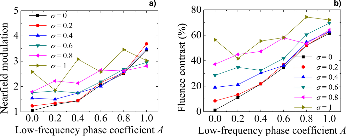
In Figure 3, it also shows that the near-field modulation and fluence contrast increase sharply when σ = 0 (i.e. wavefront without high-frequency wavefront aberrations) and the output near-field modulation is larger than 2:1 and the output fluence contrast is larger than 30% when A > 0.6. It also shows that influence degree of low-frequency wavefront distortion on the output beam quality has a certain relation with the high-frequency wavefront distortion. When high-frequency wavefront distortion is small, such as σ = 0 or 0.2, that influence degree is more obvious. That is to say, the output near-field modulation and fluence contrast increase obviously against A when σ is low.
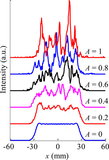
For example, Figure 4 gives the output near-field intensity distribution when σ = 0 and A = 0, 0.2, 0.4, 0.6, 0.8, and 1. It suggests that output near field worsens with low-frequency phase coefficient increasing. Low-frequency wavefront aberration changes the shape of output near-field distribution. When A > 0.6, the overall near-field profile is not uniform.
Near-field intensity distribution of input laser and output laser with σ = 0, A = 0, 0.2, 0.4, 0.6, 0.8, and 1.

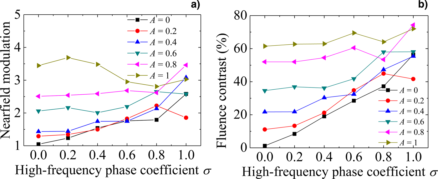
Figure 5 shows the changing trends of the near-field modulation and fluence contrast against the high-frequency wavefront distortion. Near-field modulation and fluence contrast increase with high-frequency phase coefficient, and the trend intensifies when low-frequency phase coefficient is small, such as A < 0.6. The output near-field modulation and fluence contrast of the laser beam increase sharply when A = 0 (i.e. wavefront without low-frequency wavefront aberrations), and the output fluence contrast is larger than 30% when σ > 0.6. In Figure 5, it also shows that the output near-field modulation and fluence contrast increase obviously on the whole against with σ when A is low. Combining Figure 3 with Figure 5, it can be found that when the output near-field modulation is <2:1 or the fluence contrast is <30%, the range of beam quality is more noticeable influenced by wavefront aberration, and outside this range, this effect is not obvious.
Near-field modulation (a) and fluence contrast (b) changed with high-frequency phase coefficient.
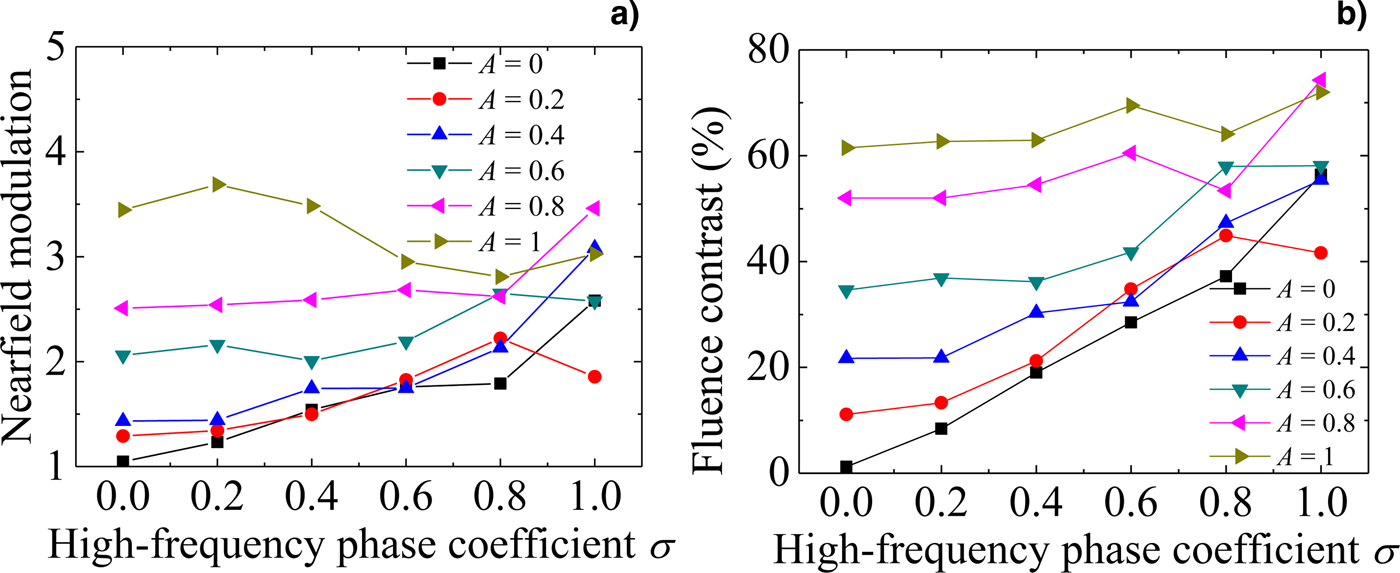
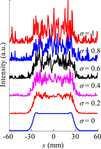
Figure 6 gives an example of the output near-field distribution in propagation when A = 0 and σ = 0, 0.2, 0.4, 0.6, 0.8, and 1. It shows that the output near field worsens with high-frequency phase coefficient increasing. Because the high-frequency wavefront aberration causes the local modulation, the near-field distribution is not uniform after propagation with the Fresnel number of 50 when the high-frequency aberration is larger, such as σ > 0.6. Combining Figure 4 with Figure 6, it can be found that the separate low frequency and high frequency have different influence on the output near-field distribution. The changing of the spatial intensity caused by the initial low-frequency wavefront distortion item is large-area modulation in the whole beam. On the other hand, the initial high-frequency distortion item caused the output spatial small-scale modulations.
Near-field intensity distribution of input laser and output laser with A = 0, σ = 0, 0.2, 0.4, 0.6, 0.8, and 1.

The analysis of the above numerical simulation results is as following. As we know, in the process of the laser propagation in free space, the spatial energy redistribution is based on the diffraction effect, which can also be seen as an interference effect. The wavefront distortion causes spatial modulation in the beam in propagation by destroying the spatial coherence of the laser. The wavefront aberration can be seen as a superposition of low frequency and high frequency. Because the low-frequency wavefront aberration represents the large-area slow-changed wavefront distribution, the degree of interference effect is small and the energy redistribution degree is relatively small in propagation. On the other hand, the energy redistribution is more frequently in spatial distribution in propagation when the high-frequency wavefront aberration exists. Therefore, the low-frequency distortion causes a slow-change spatial profile (see Fig. 4), and the high-frequency distortion causes a quick fluctuation or the small-scale modulation in the near-field profile (see Fig. 6). When the high-frequency distortion is large, the energy redistribution is relatively frequent in spatial distribution in propagation and the local high-frequency modulation becomes random. So the output near-field modulation and the fluence contrast change not obviously, and the influence degree is not obvious of the low-frequency wavefront aberration on the out near-field beam quality (see Fig. 3). When the low-frequency wavefront aberration is large, the output near-field beam quality is poor. At this condition, if loading a high-frequency wavefront distortion on this beam, the random energy redistribution would erase the inhomogeneity in the near field. Thus, when the low-frequency wavefront aberration is large, the near-field beam quality changes not obviously with the increase of high-frequency item, and even the output near-field modulation reduces [see Fig. 5(a)].
The research results above show that it is necessary to control the initial wavefront distortion to achieve a good near-field laser to meet the requirements of different applications. For example, to protect the optical components from damage, the average near-field modulation degree must satisfy M limit < 2:1 over the transmission distance of 69 m (i.e. the Fresnel number F = 50 with the beam diameter of 60 mm at 1053 nm wavelength), and we must control an appropriate initial wavefront distortion according to Figures 4(a) and 6(a). The initial wavefront distortion should be controlled with low-frequency distortion coefficient A not larger than 0.6 as well as the high-frequency distortion coefficient σ not larger than 0.6.
4. CONCLUSION
In summary, the influence of the initial wavefront distortion on the laser near-field characteristics is investigated by using numerical simulation method. The influence of low- and high-frequency wavefront aberrations on the output near-field modulation and fluence contrast is analyzed. To achieve a good near field of the flat-topped laser beam in propagation, the Fresnel number should be controlled not <50 and the low-frequency and high-frequency phase distortions must be controlled. For example, to achieve the output near-field modulation <2:1 or fluence contrast <30% at the Fresnel number F = 50, the initial wavefront distortion should be controlled with low-frequency distortion coefficient A not larger than 0.6 and high-frequency distortion coefficient σ not larger than 0.6.
ACKNOWLEDGMENTS
The authors would like to thank Dr Luoxian Zhou from Harbin Institute of Technology for valuable discussions and kind collaboration. This study was supported by the project of the National Natural Science Foundation of China under Grant No. 61622501.