1. INTRODUCTION
The Automatic Identification System (AIS) is an unattended vesselFootnote 1 reporting system that was developed for collision avoidance. The AIS transponder automatically broadcasts information on a vessel's name, position, course, speed, etc. at regular intervals to all AIS receivers in the area. Due to an International Maritime Organization (IMO) mandate (International Maritime Organization, 2002), many vessels are now directed to carry AIS systems and broadcast AIS messages. In addition to IMO requirements, some countries (Bragdon, Reference Bragdon2008) have mandated AIS be used by vessel types not required by the IMO. For some countries this includes much smaller vessels. Besides vessel-to-vessel use of AIS messages to avoid collision, the system is also used for monitoring by vessel traffic services (VTS), and by those concerned with coastal and harbour security. For AIS to be trusted in a VTS or security environment, AIS reception attributes over a domain of interest, generally termed AIS coverage, need to be understood and monitored. The coverage properties provide personnel with critical knowledge on things such as reception range, and reliable and unreliable reception areas.
The true AIS coverage is ruled by the physics of very-high frequency (VHF) propagation, power of the transmitter, etc.; however, numerical modelling of the predicted coverage, taking into account daily changes in the environment, the location of the receiver(s), etc. is a complex exercise. The complexity is prohibitive, with the results based on numerical model output as opposed to observational data.
There have been numerous published works that utilize AIS messages in research related to vessel movement. These works include the statistical analysis of lone vessel (Ristic, Scala, Morelande, et al, Reference Ristic, Scala and Morelande2008) and traffic (Aarsæther & Moan, Reference Aarsæther and Moan2009) patterns, combining AIS with surface wave radar (Ponsford, D'Souza & Kirubarajan, Reference Ponsford, D'Souza and Kirubarajan2009), and using AIS in a vessel traffic system for ensuring lane separation (Sawano, Reference Sawano2008). As well, research into the use of AIS messages to estimate AIS coverage was conducted by Baldacci (Baldacci, Reference Baldacci2008, 2010) and colleagues. The work presented here builds directly on that effort.
The working postulate is that AIS messages themselves can be used to obtain the spatial-temporal characteristics of the larger scale AIS coverage for a given geographic domain. The technique described here was first introduced in a recent paper (Lapinski & Isenor, Reference Lapinski and Isenor2010) that specifically focused on the benefits of using the technique. This paper presents the algorithm used to produce an empirical estimate of AIS coverage.
There are three objectives to the current paper:
• Give a detailed outline of the algorithm used to create the AIS coverage estimate.
• Demonstrate the usefulness of the technique using real and simulated AIS data.
• Interpret the results by showing the spatial features that the coverage estimate can illuminate.
Section 2 details the coverage estimate algorithm. Section 3 presents applications of the algorithm using synthetic and real data. Section 4 presents some concluding remarks.
2. COVERAGE ESTIMATE ALGORITHM
Plotting the location of all vessels as determined from their AIS messages represents the simplest type of AIS coverage estimate. However, this simplistic method has several deficiencies. For example, this method cannot reveal the difference between edges caused by vessels following specific routes (e.g., shipping lanes) and edges caused by a lack of reception. Also, if vessel tracks are overlapping, the simple method does not distinguish between a zoneFootnote 2 containing many vessels but having sporadic reception, and a zone with few vessels and constant reception.
The technique presented here can reveal the types of coverage characteristics noted above (Section 3). The algorithm builds on the work of Baldacci (Baldacci, Reference Baldacci2008, 2010) and colleagues by removing the temporal binning approach, modifying the definition of vessel state, and using a different expression for computing the coverage estimate. Although we consider these alterations to be improvements, we nevertheless recognize several limitations of the technique. First, the technique is unable to distinguish between the absence of reception due to no vessel being present from the absence of reception resulting from a vessel being located in an area with no AIS coverage. Second, as with any analysis using data representing past conditions, the resulting output does not necessarily represent current conditions. However, if there is sufficient vessel traffic this limitation can be minimized by reducing the time period spanned by the AIS messages used in the technique.
2.1. Terminology
To understand the algorithm, some terminology needs to be defined.
ΔA: This is a user defined spatial grid cell size. The domain of interest is divided into a grid where ΔA is the size of each grid cell. For example, a grid cell could be set with ΔA equal to 1° latitude by 1° longitude.
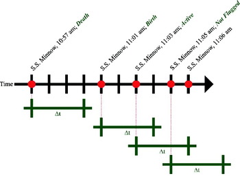
Δt: This is a user defined time interval. It is used when comparing the time difference between consecutive AIS messages from a particular vessel. Based on the comparison, a birth, active or death state is assigned to the AIS messages, as shown graphically in Figure 1.
Birth: An AIS message for a specific vessel is flagged as a birth if either of the following are true: 1) the AIS message is received from a vessel Δt or more time units after the last AIS message was received from that vessel, or 2) if it is the first AIS message received from that vessel. The former is illustrated in Figure 1 at 11:01 am on the timeline. Δt is 3 minutes in the illustration. The previous message from that vessel was 4 minutes earlier, thus the message at 11:01 is assigned the birth state.
Death: An AIS message for a vessel is flagged as a death if no subsequent AIS message is received from that specific vessel in Δt or more time units. This is illustrated in Figure 1 at 10:57 am on the timeline. The next message from the vessel is received 4 minutes later, thus exceeding the Δt of 3 minutes. Note: If the last message received from a vessel is less than Δt from the end of the dataset, the last reception is not considered a death.
Active: An AIS message for a specific vessel is flagged as active under one of the following conditions: 1) It is the next AIS message from the vessel after a birth has been assigned, and has a time stamp more than zero time units and less than Δt time units after the birth message, or 2) An AIS message is received from a different cell than the previous message, and has a time stamp less than Δt time units since the previous message from that vessel. A message cannot be flagged as active if it has been flagged as a birth or death. However, under certain circumstances one message can be flagged as both a birth and death. An example of condition 1) is illustrated in Figure 1 at 11:03 am on the timeline where the active state is assigned to a message, less than Δt minutes after a birth.
Not all messages are flagged; e.g., Figure 1 at 11:05 am on the timeline. This ensures the significance of births and deaths is not lost. If all messages were flagged, the active state would overwhelm the numbers of birth and death states. Consider the example where a vessel transmits 1000 AIS messages from a single geographic cell. The first message would be flagged as a birth. If all subsequent messages are flagged as active, the evidence that the geographic cell is proximal to a questionable reception area is lost. The birth and death messages signify that the geographic cell is in proximity to the edge of the AIS reception limit or an area with sporadic reception.
Δt concepts with message flags. The figure depicts a timeline with the AIS message times for the S.S. Minnow marked with red dots and Δt=3 minutes. The message state is written after the message time.

2.2. Assumptions
Before the algorithm is described, two assumptions should be stated: 1) it is assumed that the characteristics of AIS coverage in any area are constant over the time period of the resulting product. This means that if the product is produced from a time period of sporadic AIS reception followed by constant reception, the characteristics of the resulting coverage estimate will be an amalgamation of the two. 2) It is assumed that all AIS activity in a geographic cell represents the characteristics of AIS coverage in that geographic cell. Absence of activity in the cell is not incorporated into the calculation. This assumption seems reasonable if you consider a cell that only experiences a single vessel passing through it. If AIS messages are constantly being received from that vessel, then that cell should be shown to have good reception even if no other AIS messages are received from other vessels. Alternately, if a vessel appears in that cell and then vanishes (from a message reception perspective), then the reception characteristics in that cell should be degraded compared to the previous case.
2.3. Algorithm
The algorithm used to calculate the cell coverage estimate is as follows: After reading in the AIS data to be analyzed, defining the geographic domain over which the grid will be constructed, setting Δt and ΔA,
1. Assign each AIS report to the geographic grid cell from which it was broadcast.
2. Identify all the distinct vessels.
3. For each vessel, time sort the AIS messages.
4. Calculate the time difference between each consecutive AIS message from a vessel.
5. For each vessel, identify the consecutive AIS messages where the vessel moves from one geographic cell to another.
6. Flag messages as births, deaths and actives.
7. Count the number of flagged births (B), deaths (D) and actives (A) per geographic cell, where
 are the number of actives, births and deaths flagged in geographic cell i, respectively.
8. Calculate the proportion of the births, deaths and actives per cell using Equation (1), where X∈{B,D}:
(1)(Note that messages flagged as a birth occurring within the first Δt of the data set are not used in calculations since all vessels present will appear to be born during that time.)9. Calculate the cell coverage estimate, C i, for each geographic cell, i, using Equation (2):
(2)If in Equation (1), then C i=0.10. Plot each cell coverage estimate for the entire geographic domain using colour coding to represent the estimate values. The plot is termed the coverage estimate.
 are the number of actives, births and deaths flagged in geographic cell i, respectively.
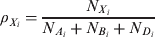

 in Equation (
Note the behaviour characteristic of Equation (2). If no AIS message was received in a cell, the cell coverage estimate is set to 0 (i.e., indicating absent or unknown AIS coverage). If only active messages have been received in a cell, the cell coverage estimate equals 1 (high estimate). If there are only births and/or deaths in a cell, the cell coverage estimate is 0·5 (i.e., low estimate, indicating vessels disappear in proximity to the cell). If there is a mixture of births, deaths and actives flagged in the cell, the cell coverage estimate will be between 0·5 and 1.
The coefficients 0·5 in Equation (2) were chosen based on the premise that C i should equal 0·5 for any combination of births and deaths in a cell (no actives present). The C i value of 0·5 represents a mid-point between no AIS coverage (C i=0) and areas with only active messages present (C i=1).
2.4. Important Algorithm Parameters
There are two important algorithm parameters that are set based on user requirements: Δt and ΔA.
The time interval parameter, Δt, should be set to a value greater than the AIS recommended reporting intervals used by the vessels in the area. Note that reporting intervals are sometimes changed during the course of a voyage. Changes can be due to vessel activity (e.g., anchored, moving) and are correlated to the class of the mobile equipment being used (e.g., Class A or B) (International Telecommunications Union, 2010). The recommended minimum report rate used by AIS transmitters is three minutes, used by vessels at anchor or moving slowly. Based on this minimum rate and timing studies through the course of this work, we advise a Δt of six minutes, twice the minimum rate. How the choice of Δt effects the coverage estimate is illustrated in Section 3.
The grid cell size, ΔA, defines the spatial resolution of the resulting coverage estimate. Choosing a large ΔA decreases computation time but diffuses the coverage estimate characteristics (see Section 3). As ΔA decreases, a point is reached where making the ΔA smaller does not add any valuable information. This happens one of two ways: 1) visually, the coverage estimate does not change by decreasing the grid size; therefore, to save computation time, it is best to use the coarser grid that gives similar results. 2) When ΔA becomes small enough, the resolution of the data becomes coarser than the grid, resulting in the potential for vessels to traverse multiple grid cells between consecutive AIS transmissions. Ideally, one would want to receive at least one AIS message from each geographic cell that a vessel passes through. If AIS transmissions are being lost, which is to be expected in poor coverage areas and at the edges of the coverage extent, the vessel should not be able to traverse through more than one cell within Δt, the acceptable amount of time between transmissions. Therefore, as a rule the ΔA should not be so small that a realistically fast cargo vessel can traverse more than one cell within the set Δt. Alternatively, in an area where all AIS messages are being received, the vessel should not be able to traverse through more than one cell between consecutive transmissions. Unless Δt is set smaller than the AIS transmission rate, the latter is likely not to happen if the former is used to limit ΔA. An automated determination of grid size has not yet been developed.
3. RESULTS
In this section the results of applying the algorithm to synthetic and real data are presented. The objectives of this section are to illustrate the algorithm's behaviour and to point out the interesting features present in the coverage estimates.
3.1. Application to Synthetic data
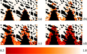
Figure 2 shows application of the algorithm to synthetic data. The domain is constructed to contain a region from which all AIS messages are received, a sinusoidal region where message reception is varied and blank zones south of the sinusoidal region from which no AIS messages are received. In the variable region, a percentage of the simulated AIS messages are randomly dropped (%drop-out).
The synthetic data contains fifty vessels that enter the region from a random point on either the lower or right edge of the domain. The synthetic vessel traverses to a random “port”, represented by a point on either the upper or left domain edge. Once reached, the synthetic vessel traverses the domain to exit at a random point on either the lower or right edge of the domain. AIS messages are transmitted from each vessel every 100 s. The vessel paths were straight lines. The vessel speeds were realistic but also randomly chosen for each vessel.
In Figure 2(a) the drop-out is 0% meaning that unless a vessel is in the blank zones, all AIS messages are received. The orange squares on the right side as well as the orange around the blank (black) zones, are from vessels entering and exiting at those cells. Every cell that is not beige or black is a cell where births and deaths have occurred. The shade is dependent on the proportion of actives that have also been counted in that cell (Equations 1 and 2).
In Figure 2(b) through (d) the drop-out around the blank zones has increased. As drop-out increases, births and deaths increase in these regions, causing the cell coverage estimates to decrease, which in turn causes the orange cells to become denser. This behaviour is essential for mapping the coverage estimate.
AIS message drop-out study using synthetic data. (a) drop-out=0%, (b) drop-out=15%, (c) drop-out=30%, (d) drop-out=70%.

3.2. The ΔA Parameter
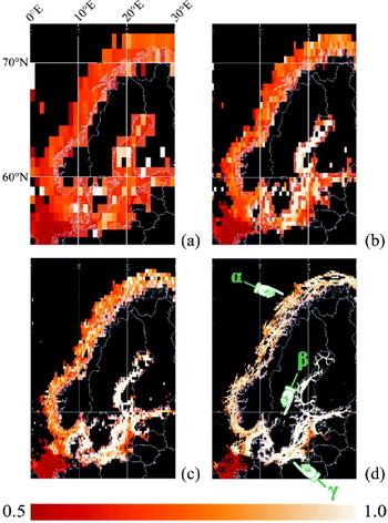
An important algorithm parameter is ΔA. Figure 3 is an example of coverage estimates where ΔA is varied. The AIS data were obtained from the Maritime Safety & Security Information System (MSSIS) (Glynn, Reference Glynn2010), an international data aggregation and distribution system for close-to-real-time AIS data. The data were collected over 24 hours in March 2010 for the region surrounding Scandinavia. The ΔA gets progressively smaller from Figure 3(a) through (d). In Figure 3(d) there are three areas labelled α, β and γ. Examining the areas α and γ in (a) through (d), shows how decreasing the grid cell size improves the spatial resolution of the coverage estimate. In both areas, as the cell size shrinks, the finer features of the coverage estimate are resolved. In the γ area, the island present in the centre of the waterway is resolved in (d) (also Figure 4, α region) as is the zone of low coverage estimate. The influence of the zones of low coverage estimate diffuse noticeably in (c) for α and γ. The area indicated by β shows how the reduction in cell size allows the resolution of finer geographic features such as lakes and rivers. In this set of examples, the grid cell size in (d) of 0·1° by 0·1° is considered to be the most appropriate.
With respect to notable features of the coverage estimate, in Figure 3(d) it can be seen that for the MSSIS data and a Δt equal to six minutes, the coverage estimate along the Norwegian coastline (e.g., α region) is a mixture of high and low estimates, while the Baltic Sea (e.g., γ region) and the Gulf of Bothnia have high estimates, with few exceptions. The coverage estimate in the Baltic Sea and Gulf of Bothnia will be examined more closely using Figure 4. In the bottom left corner there is a dominant low (red coloured) estimate zone in the North Sea. This will be examined closer using Figure 5.
ΔA study. 24 hours of Scandinavian MSSIS AIS data. Δt=360 s. (a) ΔA=1·0° by 1·0°, (b) ΔA=0·5° by 0·5°, (c) ΔA=0·25° by 0·25°, and (d) ΔA=0·1° by 0·1°. α, β, and γ point to areas of note.

3.3. The Δt Parameter
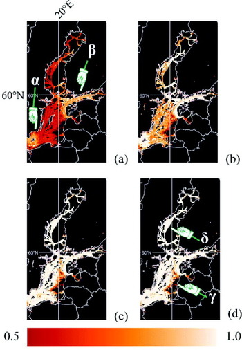
The second important parameter, Δt, is varied in Figure 4(a) through (d). The figure uses the same data used in Figure 3, but focuses on the Baltic Sea and Gulf of Bothnia areas. In Figure 4(a), Δt is one minute. At this Δt, the high coverage estimate is seen to be in the areas indicated by α and β, while the other areas either have a low estimate or have no estimate. Most vessels are recommended to be reporting at intervals of 30 s or less (International Telecommunications Union, 2010); therefore, having a low estimate is unexpected in an area such as this. However, without knowing the receiver positions for the data feeding the MSSIS, or if the institutions feeding the data to the MSSIS are decimating the data (e.g., to save bandwidth), it is difficult to make any definitive conclusions as to why the coverage estimate at this Δt is low. The temporal characteristics of the data would also be influenced if the AIS messages were being sent in a non-self-organizing manner, which is an option with base stations and could create longer gaps between messages.
In Figure 4(b), Δt has been set to three minutes. The value of the coverage estimate increases over the entire domain. The areas pointed to by α and β (in (a)) are now areas of higher coverage estimate values. At Δt equal to six minutes in (c), most areas are shown in beige indicating higher estimate values. Figure 4(d), where Δt is 11 minutes, looks nearly identical to (c). This set of figures indicates how the time difference between messages and the coverage estimate are related. Since the time difference between messages is ultimately controlled by the vessel, when utilizing the self-organizing abilities of AIS, it indirectly indicates the importance of knowing vessel compliance characteristics and how data providers (e.g., those responsible for receivers, or data aggregators such as the MSSIS) alter the temporal characteristics of the data.
Δt study. 24 hours of Baltic Sea and Gulf of Bothnia MSSIS AIS data. ΔA=0·1° by 0·1°. (a) Δt=60 s, (b) Δt=180 s, (c) Δt=360 s, (d) Δt=660 s. α, β, γ and δ point to areas of note.

3.4. Edges of no Coverage Estimate
Now consider the areas of no coverage estimate. This situation arises when there are no vessels broadcasting AIS messages or when there is no means to receive AIS messages from that area (i.e., a lack of AIS coverage). Careful examination of the coverage estimate edge can help to distinguish these two conditions, with examples of both conditions appearing in Figure 4.
If there is no means to receive AIS messages, vessels will appear in and disappear from the AIS coverage area due to them entering and exiting the area, respectively. Therefore, if Δt is large (i.e., larger than a likely data decimation time interval), such as 11 minutes in this case, only vessels that are truly appearing and disappearing in the area will be assigned births and deaths. This is shown in the γ region in Figure 4(d). Thus, an area of high coverage estimate edged in orange next to a predominantly black area is likely caused by an AIS coverage edge.
The case of no vessels broadcasting AIS messages can also be identified. If a coverage estimate edge is caused by AIS broadcasting vessels not travelling through a particular area, perhaps confined by shipping lanes or by international boundaries, at large Δt there will be no vessels appearing and disappearing at the edge. This manifests itself as an edge between an area of high coverage estimate (beige) next to a predominately black region. This can be seen in the region pointed to by δ in Figure 4(d).
3.5 Importance of input data details
As noted previously, this work used AIS data from the MSSIS. The MSSIS is an aggregator or intermediate provider, providing data from numerous source receivers, national authorities, etc. The authors have no control over and no information on the data being inputted into the MSSIS. As a result, features can appear in the coverage estimate that are difficult to explain, such as those shown in Figure 5.
Odd coverage features. 24 hours of North Sea MSSIS AIS data. ΔA=0·05° by 0·05°, Δt=360 s. α, β, γ and δ point to areas of note.

Figure 5 shows 24 hours of data from about 4000 distinct vessels. Four features of interest have been labelled. Firstly, α points to a large zone in the North Sea where the coverage estimate is predominantly close to 0·5. Given the size of the zone, and the distinct northern edge of the feature, it seems unlikely to be a naturally occurring phenomenon. Instead the authors presume that whoever is supplying these data to the MSSIS is decimating the data to a time interval greater than six minutes (and greater than 11 minutes, figure not shown). Whatever the cause, α shows how the coverage estimate can illuminate a zone that has poor reception even though it has a large number of AIS messages. Note that if instead of the coverage estimate, one plotted the positions of all received AIS messages, one would likely get the impression of reliable and timely reception in the area. The coverage estimate, which incorporates temporal influences into the visual product, exposes the unreliable nature of data delivery in the area.
On the edge of this low coverage estimate zone, β points to a region that has a higher coverage estimate. This likely means there is a receiver in that area providing data to the MSSIS separate from the other data. The region indicated by γ is also interesting. This area of elevated coverage estimate is well removed from land and has a distinctive circular appearance, suggesting an offshore receiver. Finally, δ points to a suspicious blank zone along the coast of Germany. This could be due to a lack of receivers in the area (it is difficult to deduce with the red zone right next to it). Also, this blank zone has a distinctive sharp and straight edge at the Germany-Denmark border. The edge has characteristics consistent with an end of AIS coverage; however, the straightness of the edge (Mercator map projection) suggests a very large radius from a single AIS receiver (unlikely) or multiple receivers in the area (more likely). Alternatively, it could be a result of selective data omission. Those supplying data to the MSSIS about vessels in Denmark's water may be selectively removing AIS data from Germany's territorial water. Such mysteries are a direct result of using data from a provider when little or no information about the originating data source is available.
3.6. Examining the Total Time Period used in the Coverage Estimate
Thus far, results have been shown in areas with many vessels broadcasting AIS messages. We now present results in domains of interest with considerably fewer AIS transmitting vessels in a smaller domain of interest to show how the algorithm behaves in these environments and to show other aspects of the coverage estimate method.
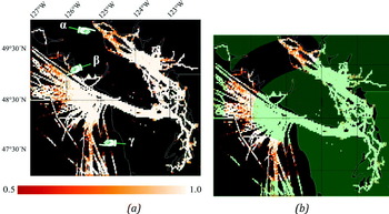
Figures 6 and 7 show the coverage estimates for a domain of interest that is off the coast of Vancouver Island, Canada and north-west Washington State, USA. In Figure 7, the blue boxes indicate the data collection area. Figure 6(a) shows a coverage estimate using seven days of AIS data, for March 10 through 16, 2010. 640 distinct vessels transmitted during that time. The average number of distinct vessels in each of the 24 hour periods was 395, skewed slightly low due to the smaller data collection area on the first day. For an area of approximately 3 degrees latitude and 5 degrees longitude, 395 appears to be a reasonable number of ships to get a usable coverage estimate.
Seven days of Northeast Pacific MSSIS AIS data, March 2010. ΔA = 0.025° by 0.025°, Δt = 360s. (a) & (b) are the same figure with the exception that (b) circles an area of interest. 640 distinct vessels. α, β, γ and δ point to areas of note.

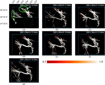
A week of one day coverage estimates for the Northeast Pacific. ΔA=0·025° by 0·025°, Δt=360 s. (a) March 10, 2010; 232 distinct vessels. (b) March 11, 2010; 418 distinct vessels. (c) March 12, 2010; 429 distinct vessels. (d) March 13, 2010; 407 distinct vessels. (e) March 14, 2010; 402 distinct vessels. (f) March 15, 2010; 438 distinct vessels. (g) March 16, 2010; 439 distinct vessels. The blue box indicates the data collection area.

Figure 6 and 7 will help illustrate the care that must be taken when choosing the time window used for the coverage estimate. Looking at Figure 6(a), we note that the estimate is generally high with the exception of α, β and γ. All three locations indicate zones of reduced coverage estimate. Also, the β zone has high coverage estimate zones on both sides of the reduced coverage estimate. An initial explanation could be that two coverage areas are meeting at these locations. However, examination of the daily coverage estimate will illustrate that the spatial arc (highlighted in Figure 6(b)) formed by α, β and γ (Figure 6(a)) is the cause of the reduced coverage in these zones.
In Figure 7, (a) through (g) represent coverage estimates for each day from March 10 to March 16, 2010. Note that the data collection area was smaller on March 10 (Figure 7(a)) than on the other six days. When the coverage estimate touches the data collection bounding box, it means the extent of the AIS reception was likely beyond the extent of the data collection area.
In Figure 7(a), an area is circled and labelled α. If this same area is examined in Figure 7(a) through (g), it can be seen that the coverage estimates extend further north-west in (a), (b) and (g) as compared to other days. In (c) through (f), the coverage estimates do not reach the bounding box in the α area. In (c) through (f) α area, the coverage estimate decreases from high to low before reaching an area with no estimate, a sign that there are no means to receive AIS messages near the bounding box edge at this location on those days, and thus suggesting an AIS coverage edge. Examining the Figure 7 β zone (see Figure 7a), it can be seen that the coverage estimate touches the western boundary in (a), (b) and (g) unlike on the other days. Again, on the other days, the coverage estimate characteristics indicate an edge to the AIS reception capabilities is being observed. The fluctuations in the coverage extent, in the α and β areas, are the cause of the reduced coverage indicated in Figure 6, that figure showing the coverage estimate calculated using all seven days of data.
The figures illustrate the implications of a long time window being used for the coverage estimate. The daily fluctuations in coverage were lost in Figure 6 by using seven days of data to produce a single, composite product. The result is a misleading coverage estimate. In this particular case, the misleading estimate suggests a coverage which is not realistic for any one day, but rather is a temporal composite of the total time period. This is not to say that multiple day coverage estimates should not be made. Rather, we recognize that producing daily coverage estimates in addition to the multi-day estimate would be a wise practice. The daily estimates would help ensure that no major daily fluctuations were occurring that could detrimentally skew the multi-day estimate. With regards to the fluctuations, it is possible that changing environmental conditions or non-functioning AIS receivers are the cause. Further analysis of this feature is ongoing.
3.7. Minimal Vessels and the Coverage Estimate
To investigate the implications of a small number of AIS broadcasting vessels, consider data collected over a week in March 2010 for Halifax Harbour, Halifax, Canada. The area of interest covers approximately 10 minutes of latitude by 10 minutes of longitude. Over that week only 44 distinct vessels reported in the domain of interest, based on the AIS data obtained from the MSSIS. An average of 22·6 distinct vessels reported daily. Although this is a low number, it does not necessarily mean the coverage estimate will not be useful. The estimate is not dependent on the number of distinct vessels but rather it is dependent on the area traversed by the vessels in the domain of interest from which messages are received. In this regard, one vessel broadcasting AIS messages and sailing over the entire domain of interest could provide a complete coverage estimate for the domain.
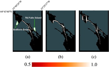
The coverage estimates, computed for three individual days for Halifax Harbour, are shown in Figure 8(a) to (c). Examining the Bedford Basin area, note how there are births/deaths consistently occurring in the northwest zone of the Basin (indicated by the orange zone). This is an area where ships moor, waiting for available port facilities. It is conceivable vessels in this area are cycling their power or AIS transmitter, thus affecting the AIS transmission rate.
Example of one day coverage estimates for the Halifax Harbour. ΔA=0·001° by 0·001°, Δt=360 s. (a) March 11, 2010; 26 distinct vessels. (b) March 14, 2010; 20 distinct vessels. (c) March 15, 2010; 19 distinct vessels.

In Figure 8(a), note that the edge of the coverage estimate near the mouth of the basin (where the narrow waterway broadens into the Basin area) indicates excellent (consistent) reception. In (b) and (c) there are similarly high cell coverage estimates within the basin with no sign of an edge to the coverage extent. What this indicates in these and the other days of this week (not shown here) is that activity from AIS transmitting vessels in the basin varies on a daily basis. The absence of coverage estimates in the basin is due to traffic variability not coverage variability. Again, these figures show how the coverage estimate may be used to distinguish edges due to AIS reception limits from edges due to a lack of vessels.
The southern extent of the coverage estimates do vary significantly from day to day. Halifax Harbour has defined shipping lanes which become evident in coverage estimates south of McNabs Island. When the southern extent of the coverage estimates change, it is likely an indication that AIS reception range is changing, which is reinforced by the low coverage estimate cells at the southern extent of the domain.
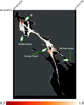
The daily coverage estimates from the March 2010 week indicate consistent coverage for most of the harbour, the exception being the southern region. Given this consistency, a composite using the entire week's data would be a useful product. Figure 9 shows the seven day coverage estimate for the Harbour. The composite emphasises many of the features described for Figure 8, including the mooring area in Bedford Basin, the coastline docking areas, and to a lesser extent the fading of reception in the southern harbour.
Seven day coverage estimate for Halifax Harbour during March 2010. ΔA=0·001° by 0·001°, Δt=360 s. α points to an area of note.

4. CONCLUSIONS
AIS messages can be used to obtain the spatial-temporal characteristics of AIS coverage for a given geographic domain by using the algorithm detailed in this paper and choosing appropriate algorithm parameter values. We have shown how the coverage estimate changes with AIS message loss and how the Δt and ΔA parameters influence the output. Of significance is how the time interval between messages, relative to Δt, impacts the coverage estimate. This indicates that knowledge on whether AIS messages are being broadcast in a manner not recommended by the ITU or if the data have been temporally decimated is valuable for such an analysis. We have also shown how the edges of the coverage estimate technique can be used to distinguish between the absence of vessels as compared to an actual edge in the AIS coverage. The technique was also seen to be useful in identifying zones of poor AIS reception even in high traffic areas. The use of data sets that extend over multiple days was shown to have a possible adverse effect on the coverage estimate, producing an average estimate that does not properly represent any particular time within the time period of the data set. However, in areas where the coverage does not vary significantly from day to day it was shown that coverage estimates created using data from multiple days can be valuable, particularly in areas of interest that have minimal vessel traffic using AIS.
ACKNOWLEDGEMENT
The authors would like to thank Sean Webb for supplying the technical support required to establish and acquire the necessary data and Alberto Baldacci for his helpful information on the work he and his colleagues conducted.