1 Introduction
Buoyant jets and plumes arise when a fluid of lower density is released into a higher uniform or stratified ambient density field. The study of buoyant jets and plumes received considerable attention in the past since these simpler flow configurations serve as models for understanding complex dynamics in several flows that occur in nature and in engineering practice, for example atmospheric thermals, mantle plumes, release of flue gases from smoke stacks, pool fires, diffusion flames, hot jets, fuel leaks etc. The ratio of buoyancy to inertial forces, i.e. the Richardson number, determines the parameter that broadly classifies buoyant jets and plumes. The inlet Richardson number is defined as
 $Ri_{0}=(\unicode[STIX]{x1D70C}_{\infty }-\unicode[STIX]{x1D70C}_{0})gD/\unicode[STIX]{x1D70C}_{0}V_{0}^{2}$
, where
 $\unicode[STIX]{x1D70C}$
,
 $V$
and
 $D$
are density, velocity, and source diameter respectively,
 $g$
is the acceleration due to gravity, subscripts
 $0$
and
 $\infty$
correspond to the source and ambient conditions respectively in this paper. For
 $Ri_{0}\ll 1$
, the release at the inlet is momentum dominated with negligible buoyancy and is hence referred to as a buoyant jet, while for
 $Ri_{0}\gg 1$
, the release becomes buoyancy dominated and is hence referred to as a buoyant plume. Nevertheless, a buoyant jet gradually loses its momentum and achieves buoyant plume behaviour in the far field.
In buoyant plumes, earlier investigations had revealed that below a certain inlet density ratio
 $S=\unicode[STIX]{x1D70C}_{0}/\unicode[STIX]{x1D70C}_{\infty }$
, these plumes exhibit a self-sustained periodic oscillatory instability close to their origin. These oscillations result in the formation and downstream convection of a large-scale toroidal vortex in a cyclic manner, a phenomenon commonly termed puffing (Cetegen & Kasper Reference Cetegen and Kasper1996). Self-sustained oscillations are also observed in buoyancy dominant flows such as pool fires (Cetegen & Ahmed Reference Cetegen and Ahmed1993) and buoyant diffusion flames (Cetegen & Dong Reference Cetegen and Dong2000; Moreno-Boza et al.
Reference Moreno-Boza, Coenen, Sevilla, Carpio, Sánchez and Liñán2016), a classic example being the flickering instability observed in a candle flame (Maxworthy Reference Maxworthy1999). The study of puffing in buoyant plumes and fires received considerable attention since the vortical structures that arise from puffing act as the primary mechanism by which these flows entrain ambient fluid near the source (Cetegen Reference Cetegen1998). More importantly, in fires and flames, puffing enhances the oxygen supply, which affects the combustion process in the source vicinity.
Several researchers have studied the puffing in buoyant plumes in the past by simulating them using release of helium and helium–air mixtures into the air. Subbarao & Cantwell (Reference Subbarao and Cantwell1992) measured puffing frequencies in moderate
 $Ri_{0}$
range 0.1–7 that extended from jet to plume regime by independently varying the Reynolds number
 $Re$
and the Richardson number
 $Ri_{0}$
. They found that the non-dimensional frequency i.e. Strouhal number
 $St$
, is independent of
 $Re$
and is only a function of
 $Ri_{0}$
. The Reynolds number and the Strouhal number are defined as
 $Re=\unicode[STIX]{x1D70C}_{0}V_{0}D/\unicode[STIX]{x1D707}_{0}$
and
 $St=fD/V_{0}$
respectively, where
 $f$
is the frequency. However, as the plumes approach jet regime, the
 $St$
attains an approximately constant value independent of both
 $Re$
and
 $Ri_{0}$
. They reported that this transition from jet to plume regime occurs over
 $Ri_{0}$
range between 0.5 and 1. Much of the earlier work in investigating puffing characteristics of low-density gas plumes was reported by Cetegen and his co-authors. Cetegen & Ahmed (Reference Cetegen and Ahmed1993) investigated the mechanism by which the oscillations become self-sustained by introducing various disturbances/modifications near the plume source. They observed that the perturbations induced by the downstream convecting vortex act as a feedback mechanism to trigger instability near the plume origin which repeats in a cyclic manner. Thus, they concluded that the puffing frequencies in plumes are connected to the convection velocity of the puffing vortices. Further, Cetegen & Kasper (Reference Cetegen and Kasper1996) extensively investigated buoyant plumes for a large range of nozzle diameters, source velocities and plume densities, and found that the puffing frequency dependence on inlet conditions can be well represented by a power-law variation between
 $St$
and a modified form of Richardson number
 $Ri=(\unicode[STIX]{x1D70C}_{\infty }-\unicode[STIX]{x1D70C}_{0})gD/\unicode[STIX]{x1D70C}_{\infty }V_{0}^{2}$
. In the
 $Ri$
range investigated (0.2–7000), they obtained two power laws
 $St=0.8Ri^{0.38}$
for
 $Ri<100$
and
 $St=2.1Ri^{0.28}$
for
 $Ri>500$
. They attributed this transition in frequency scaling to the transition in puffing from laminar to a more vigorously mixed turbulent state within the
 $Ri$
range 100–500. Furthermore, Cetegen (Reference Cetegen1997) performed a series of experiments and mapped the stability boundary between laminar and puffing plumes on the
 $Re{-}S$
plane. They found that for a fixed inlet density, the steady laminar plumes turn pulsating/puffing only beyond a minimum threshold inlet velocity. Also, they found that the puffing instability ceases to occur above density ratios
 $S=\unicode[STIX]{x1D70C}_{0}/\unicode[STIX]{x1D70C}_{\infty }=0.5{-}0.6$
. However, their stability diagram did not take into account the effect of Froude number,
 $Fr=V_{0}/\sqrt{gD}$
, on plume transition. Jiang & Luo (Reference Jiang and Luo2000a
) and Jiang & Luo (Reference Jiang and Luo2000b
) investigated the puffing phenomenon in buoyant thermal plumes by performing direct numerical simulations in an axisymmetric domain. They could effectively reproduce puffing in axisymmetric thermal plumes and their results corroborated those of the earlier experiments in helium plumes, which lead to the conclusion that puffing is an axisymmetric instability. Jiang & Luo (Reference Jiang and Luo2000a
) observed that the puffing diminished when gravity was artificially reduced and concluded that plume puffing is a result of buoyancy instability of the fluid itself, which arises because of the action of gravity on the radial density stratification near the plume inlet (gravitational torque). Similar investigations were performed in planar helium–air plumes by Cetegen, Dong & Soteriou (Reference Cetegen, Dong and Soteriou1998) and Soteriou, Dong & Cetegen (Reference Soteriou, Dong and Cetegen2002), and in planar thermal pure plumes by Hattori et al. (Reference Hattori, Bartos, Norris, Kirkpatrick and Armfield2013a
) and Hattori et al. (Reference Hattori, Norris, Kirkpatrick and Armfield2013b
).
The primitive non-dimensional groups that govern the buoyant jet/plume dynamics are
 $Re$
,
 $Fr$
and
 $S$
(Soteriou et al.
Reference Soteriou, Dong and Cetegen2002). In spite of the findings, a major drawback in the plume experiments is the inability to independently vary the non-dimensional groups to investigate the effect of each group on the puffing phenomenon. In experiments, the plume conditions can only be altered by varying any of the three inlet control parameters
 $D$
,
 $V_{0}$
and
 $\unicode[STIX]{x1D70C}_{0}$
, which leads to a simultaneous variation of two non-dimensional groups. For example, varying
 $\unicode[STIX]{x1D70C}_{0}$
modifies
 $Re$
and
 $S$
simultaneously, while varying
 $V_{0}$
or
 $D$
modifies
 $Re$
and
 $Fr$
simultaneously. Thus, it is difficult to explore plume behaviour in the whole
 $Re{-}Fr{-}S$
space using experiments. Alternatively, linear stability analysis serves as an effective tool for such extensive parametric investigation (for example, Nichols, Schmid & Riley (Reference Nichols, Schmid and Riley2007) in the case of buoyant jets).
In spite of the negligible effects of buoyancy, self-sustained oscillations are also observed in the near field of momentum dominated helium jets (Sreenivasan, Raghu & Kyle Reference Sreenivasan, Raghu and Kyle1989; Kyle & Sreenivasan Reference Kyle and Sreenivasan1993) and hot jets (Monkewitz et al.
Reference Monkewitz, Bechert, Barsikow and Lehmann1990) for density ratios
 $S<0.6$
. The linear stability analysis using local spatio-temporal theory in parallel buoyant jets attributed the reason for these global oscillations to the presence of absolute instability in the jet base flow (Monkewitz & Sohn Reference Monkewitz and Sohn1988). In buoyant jets, local instability analysis had been widely applied to investigate the importance of various source parameters (Lesshafft & Huerre Reference Lesshafft and Huerre2007; Nichols et al.
Reference Nichols, Schmid and Riley2007; Srinivasan, Hallberg & Strykowski Reference Srinivasan, Hallberg and Strykowski2010; Coenen & Sevilla Reference Coenen and Sevilla2012) and effect of co-flow or counter flow on these global oscillations (Hallberg et al.
Reference Hallberg, Srinivasan, Gorse and Strykowski2007). More importantly, Nichols et al. (Reference Nichols, Schmid and Riley2007) demonstrated a good agreement between the absolutely unstable mode frequency obtained from local analysis and the global mode frequency from direct numerical simulation and further investigated the effect of various non-dimensional groups on jet instability. However, all these investigations are confined to the buoyant jet regime (
 $Ri_{0}\ll 1$
).
In buoyant plumes, the earlier linear stability analysis investigations were confined to smaller density gradients in which the governing equations were simplified using the Boussinesq approximation. Further, these investigations were largely confined to either spatial or temporal analysis in the self-similar region of a laminar plume (Mollendorf & Gebhart Reference Mollendorf and Gebhart1973; Wakitani Reference Wakitani1980; Riley & Tveitereid Reference Riley and Tveitereid1984). These analyses revealed that the far-field self-similar region of a plume is convectively unstable for helical perturbations (
 $m=1$
), and remains stable for axisymmetric (
 $m=0$
) and double helical perturbations (
 $m=2$
). Also, Riley & Tveitereid (Reference Riley and Tveitereid1984) found that the helical instability in these plumes stabilizes by the imposition of a co-flowing stream around the plume. Further, Tveitereid & Riley (Reference Tveitereid and Riley1992) estimated the critical
 $Re$
for the onset of helical instability as 43 and found that its value increases with an increase in the co-flow velocity. More recently, Chakravarthy, Lesshafft & Huerre (Reference Chakravarthy, Lesshafft and Huerre2015) investigated both near-field and far-field self-similar regions in Boussinesq thermal plumes and found that both regions exhibit absolute instability only for the helical mode. Their result is in contrast to the helium plume experiments in which the instability observed is only axisymmetric. They attributed this difference to the use of Boussinesq approximation which is not valid for such a low density ratio helium/helium–air plumes.
To further address this difference and ascertain the role of non-Boussinesq effects, Chakravarthy (Reference Chakravarthy2015), Chakravarthy, Lesshafft & Huerre (Reference Chakravarthy, Lesshafft, Huerre and Segalini2016) and Huerre, Chakravarthy & Lesshafft (Reference Huerre, Chakravarthy, Lesshafft and Floryan2016) investigated the linear global stability of laminar hot jets and thermal plumes under the low Mach number approximation. They found that only axisymmetric perturbations exhibit global instability, while helical perturbations are globally stable. Their linear predictions are in reasonably good agreement with the earlier experiments, which shows that the non-Boussinesq effects indeed play a major role in governing the global dynamics of buoyant jets and plumes. Through a sensitivity analysis, they estimated the contribution of various forces in the momentum equation to the destabilization of buoyant jets and plumes. In buoyant jets, they identified the base flow shear to be the main destabilizing force and found that gravity has a negligible effect on global instability in the buoyant jet regime. In plumes, they identified the buoyancy to be the main destabilizing force. Further, through local spatio-temporal analysis, they established the presence of a larger region of absolute instability in the vicinity of buoyant jet/plume inlet for
 $m=0$
and concluded that these global oscillations are intrinsic to these low-density flows, and they do not arise as a result of any forcing at boundaries.
Overall, as seen from the literature, the near-field oscillatory instability in jets had been extensively investigated using linear stability analysis, while such investigations are limited in plumes. While the work of Chakravarthy (Reference Chakravarthy2015) draws important conclusions and explains some of the observations found in earlier plume experiments, their investigations are confined only to two Reynolds numbers 400 and 1000. Thus, the earlier plume investigations lack a comprehensive parametric study that considers the effect of various non-dimensional parameters on plume instability. Further, in the plume regime, the global stability computations of Chakravarthy (Reference Chakravarthy2015) are limited to
 $Ri<500$
. The experiments of Cetegen & Kasper (Reference Cetegen and Kasper1996) observed a change in global dynamics of plumes for
 $Ri>500$
, where puffing becomes turbulent and undergoes a switch in frequency scaling. Therefore, it is important to investigate plumes of higher
 $Ri$
whose global behaviour seems to differ from that of lower
 $Ri$
plumes. The present investigation aims to address these issues by employing global linear stability analysis and experiments. Unlike buoyant jets, the near field of buoyant plumes is highly non-parallel because of the stronger buoyant acceleration along the centreline, accompanied by a predominant radial inflow towards the centreline (refer to figures 2 and 3). In such cases, the parallel flow assumption is no longer valid as shown by Chakravarthy (Reference Chakravarthy2015) and hence, the present work employs global linear instability analysis for non-parallel, two-dimensional base flow using the approach outlined in Theofilis (Reference Theofilis2003). Further, the density contrast in Chakravarthy (Reference Chakravarthy2015) is due to the temperature differences, which has presented some differences in their instability characteristics when compared to the helium/helium–air plumes of Cetegen & Kasper (Reference Cetegen and Kasper1996). Therefore, the present work aims to investigate the instability characteristics of plumes of helium and helium–air mixtures. Nevertheless, the present parameter space is largely confined to the plume regime while Chakravarthy (Reference Chakravarthy2015) explored more fully the transition from buoyant jet to plume regime.
Using global linear stability analysis, the effect of various non-dimensional groups on plume instability is considered. Further, the modes for which the plumes turn unstable are identified and transition maps and frequency scaling laws for these unstable modes have been obtained. Next, we explored the effect of the inlet velocity profile on plume oscillation frequency and transition. Finally, by deriving an equation for perturbation vorticity in variable-density flows and following an approach similar to that of Lesshafft & Huerre (Reference Lesshafft and Huerre2007), we investigated the perturbation vorticity mechanisms responsible for this oscillatory instability. An attempt has been made to qualitatively explain the observed growth rate dependency on various non-dimensional parameters using these destabilization mechanisms. Additionally, experiments are performed using helium and helium–air mixtures releasing into the air from circular orifices and pipe nozzles in order to validate the results of the linear stability analysis. An experimental set-up has been designed carefully to minimize the disturbances generally present in such experiments to address discrepancies observed between the present linear analysis and the earlier plume experiments. The details regarding the global instability analysis and experiments are given in §§ 2 and 3 respectively.
2 Global linear stability analysis
2.1 Governing equations
The stability characteristics of isothermal, variable-density gas plumes of helium and helium–air mixtures emanating into a quiescent ambient air from circular inlets are investigated using global linear stability analysis. These plumes with source density, velocity, viscosity and helium mass fraction
 $\unicode[STIX]{x1D70C}_{0}$
,
 $V_{0}$
,
 $\unicode[STIX]{x1D707}_{0}$
and
 $Y_{He0}$
respectively eject out of a circular source of diameter
 $D$
into a still ambient air of constant density
 $\unicode[STIX]{x1D70C}_{\infty }$
and viscosity
 $\unicode[STIX]{x1D707}_{\infty }$
. Since the density differences between the plume source and the ambient are significant, the Boussinesq approximation is not applicable for these plumes. For such flows, the governing equations are the compressible continuity, momentum, species transport and state equations simplified in the low Mach number limit (Nichols et al.
Reference Nichols, Schmid and Riley2007; Chandler et al.
Reference Chandler, Juniper, Nichols and Schmid2012). These equations account for the density variations due to the mixing of different species, or due to temperature, but neglect density variations because of pressure (compressibility). These equations in the non-dimensional form are given as
 $$\begin{eqnarray}\displaystyle & \displaystyle {\displaystyle \frac{\unicode[STIX]{x2202}\unicode[STIX]{x1D70C}}{\unicode[STIX]{x2202}t}}+\unicode[STIX]{x1D735}\boldsymbol{\cdot }(\unicode[STIX]{x1D70C}\boldsymbol{v})=0, & \displaystyle\end{eqnarray}$$
 $$\begin{eqnarray}\displaystyle & \displaystyle \!\!\unicode[STIX]{x1D70C}\!\left(\!{\displaystyle \frac{\unicode[STIX]{x2202}\boldsymbol{v}}{\unicode[STIX]{x2202}t}}+\boldsymbol{v}\boldsymbol{\cdot }\unicode[STIX]{x1D735}\boldsymbol{v}\!\right)=-\unicode[STIX]{x1D735}p+{\displaystyle \frac{S}{Re\,\unicode[STIX]{x1D707}^{\ast }}}\!\left\{\!\unicode[STIX]{x1D735}\boldsymbol{\cdot }[\unicode[STIX]{x1D707}(\unicode[STIX]{x1D735}\boldsymbol{v}+\unicode[STIX]{x1D735}\boldsymbol{v}^{\text{T}})]-{\displaystyle \frac{2}{3}}\unicode[STIX]{x1D735}(\unicode[STIX]{x1D707}\unicode[STIX]{x1D735}\boldsymbol{\cdot }\boldsymbol{v})\!\right\}+(1-\unicode[STIX]{x1D70C}){\displaystyle \frac{1}{Fr^{2}}}\boldsymbol{e}_{\boldsymbol{z}}, & \displaystyle \nonumber\\ \displaystyle & & \displaystyle\end{eqnarray}$$
 $$\begin{eqnarray}\displaystyle & \displaystyle \unicode[STIX]{x1D70C}\left({\displaystyle \frac{\unicode[STIX]{x2202}Y_{He}}{\unicode[STIX]{x2202}t}}+\boldsymbol{v}\boldsymbol{\cdot }\unicode[STIX]{x1D735}Y_{He}\right)={\displaystyle \frac{1}{Re\,Sc}}\unicode[STIX]{x1D735}\boldsymbol{\cdot }(\unicode[STIX]{x1D70C}\unicode[STIX]{x1D735}Y_{He}), & \displaystyle\end{eqnarray}$$
 $$\begin{eqnarray}\displaystyle & \displaystyle {\displaystyle \frac{1}{\unicode[STIX]{x1D70C}}}=\left({\displaystyle \frac{1}{S}}-1\right)Y_{He}+1. & \displaystyle\end{eqnarray}$$
Equation (2.4) shows the state equation for isothermal, isobaric (constant thermodynamic pressure) flow which gives the dependence of density on mass fraction. The composition dependence of viscosity is modelled using Wilke’s formula obtained from kinetic theory (Wilke Reference Wilke1950):
 $$\begin{eqnarray}\displaystyle \left.\begin{array}{@{}l@{}}\unicode[STIX]{x1D707}=\unicode[STIX]{x1D707}_{He/A}^{\ast }{\displaystyle \frac{1}{1+{\displaystyle \frac{Y_{He0}^{-1}-Y_{He}}{Y_{He}}}\unicode[STIX]{x1D719}_{He-A}}}+{\displaystyle \frac{1}{1+{\displaystyle \frac{Y_{He}}{Y_{He0}^{-1}-Y_{He}}}\unicode[STIX]{x1D719}_{A-He}}},\\ \qquad \text{where},~\unicode[STIX]{x1D719}_{He-A}\text{ and }\unicode[STIX]{x1D719}_{A-He}\text{ are constants defined as }\\ \unicode[STIX]{x1D719}_{He-A}={\displaystyle \frac{M_{He}}{M_{A}}}{\displaystyle \frac{\left[1+\sqrt{{\displaystyle \frac{\unicode[STIX]{x1D707}_{He}}{\unicode[STIX]{x1D707}_{A}}}}\left({\displaystyle \frac{M_{A}}{M_{He}}}\right)^{1/4}\right]^{2}}{\sqrt{8\left(1+{\displaystyle \frac{M_{He}}{M_{A}}}\right)}}},\\ \unicode[STIX]{x1D719}_{A-He}={\displaystyle \frac{M_{A}}{M_{He}}}{\displaystyle \frac{\left[1+\sqrt{{\displaystyle \frac{\unicode[STIX]{x1D707}_{A}}{\unicode[STIX]{x1D707}_{He}}}}\left({\displaystyle \frac{M_{He}}{M_{A}}}\right)^{1/4}\right]^{2}}{\sqrt{8\left(1+{\displaystyle \frac{M_{A}}{M_{He}}}\right)}}},\\ \text{and}\quad \unicode[STIX]{x1D707}_{He/A}^{\ast }={\displaystyle \frac{\unicode[STIX]{x1D707}_{He}}{\unicode[STIX]{x1D707}_{A}}}=1.073.\end{array}\right\} & & \displaystyle\end{eqnarray}$$
The mass diffusivity is assumed to follow
 $\unicode[STIX]{x1D70C}_{0}{\mathcal{D}}\approx \text{const}.$
, similar to that of Soteriou et al. (Reference Soteriou, Dong and Cetegen2002). Equations (2.1)–(2.5) form the governing equations for the present study. These equations are considered in cylindrical polar coordinates
 $(r,\unicode[STIX]{x1D703},z)$
, where
 $\boldsymbol{v}=(v_{r},v_{\unicode[STIX]{x1D703}},v_{z})$
is the velocity,
 $\unicode[STIX]{x1D70C}$
,
 $p$
,
 $Y_{He}$
,
 $\unicode[STIX]{x1D707}$
and
 $M$
are density, pressure, helium mass fraction, viscosity and molar mass respectively. Also, the subscripts
 $He$
and
 $A$
corresponds to helium and air respectively.
2.2 Non-dimensionalization
Since it is possible to non-dimensionalize the governing equations using several scales, it is important to specify the scales used to obtain dimensionless groups in (2.1)–(2.5). The primitive variables are non-dimensionalized as
 $$\begin{eqnarray}\left.\begin{array}{@{}c@{}}\boldsymbol{v}={\displaystyle \frac{\tilde{\boldsymbol{v}}}{V_{0}}},\quad Y_{He}={\displaystyle \frac{{\tilde{Y}}_{He}}{Y_{He0}}},\quad p={\displaystyle \frac{\tilde{p}}{p_{\infty }}},\quad \unicode[STIX]{x1D70C}={\displaystyle \frac{\tilde{\unicode[STIX]{x1D70C}}}{\unicode[STIX]{x1D70C}_{\infty }}},\quad \unicode[STIX]{x1D707}={\displaystyle \frac{\tilde{\unicode[STIX]{x1D707}}}{\unicode[STIX]{x1D707}_{\infty }}},\\ \unicode[STIX]{x1D735}=D\tilde{\unicode[STIX]{x1D735}},\quad t={\displaystyle \frac{\tilde{t}V_{0}}{D}},\quad \boldsymbol{g}={\displaystyle \frac{\tilde{\boldsymbol{g}}}{g}}=-\boldsymbol{e}_{\boldsymbol{z}}.\end{array}\right\}\end{eqnarray}$$
The non-dimensional equations thus obtained using the above scalings reveal the set of non-dimensional parameters that govern the plume dynamics. This set consists of Reynolds number
 $Re$
, Froude number
 $Fr$
, density ratio
 $S$
, viscosity ratio
 $\unicode[STIX]{x1D707}^{\ast }$
and Schmidt number
 $Sc$
in the following form
 $$\begin{eqnarray}Re={\displaystyle \frac{\unicode[STIX]{x1D70C}_{0}V_{0}D}{\unicode[STIX]{x1D707}_{0}}},\quad Fr={\displaystyle \frac{V_{0}}{\sqrt{gD}}},\quad S={\displaystyle \frac{\unicode[STIX]{x1D70C}_{0}}{\unicode[STIX]{x1D70C}_{\infty }}},\quad \unicode[STIX]{x1D707}^{\ast }={\displaystyle \frac{\unicode[STIX]{x1D707}_{0}}{\unicode[STIX]{x1D707}_{\infty }}},\quad Sc={\displaystyle \frac{\unicode[STIX]{x1D707}_{0}}{\unicode[STIX]{x1D70C}_{0}{\mathcal{D}}}},\end{eqnarray}$$
where,
 $g$
and
 ${\mathcal{D}}$
are acceleration due to gravity and mass diffusivity respectively. It is a common practice to combine the effects of
 $Fr$
and
 $S$
into a single buoyancy controlling non-dimensional parameter, the Richardson number
 $Ri=(1-S)Fr^{-2}$
or
 $Ri_{0}=(1/S-1)Fr^{-2}$
. However, the non-dimensionalization does not strictly support this as it does not yield
 $Ri$
or
 $Ri_{0}$
directly as a single parameter in (2.1)–(2.5) (Soteriou et al.
Reference Soteriou, Dong and Cetegen2002). While the density ratio signifies the magnitude of density difference, the Froude number signifies the effect of gravity i.e. it provides information regarding the magnitude of inertial forces compared to buoyancy forces. For example, in spite of higher density difference, higher Froude number can result in negligible buoyancy forces compared to inertial forces and vice versa. Therefore, instead of lumping into a single parameter, the present study treats the
 $Fr$
and
 $S$
effects separately as done by Soteriou et al. (Reference Soteriou, Dong and Cetegen2002) and Nichols et al. (Reference Nichols, Schmid and Riley2007), without limiting the generality.
2.3 Formulation for global linear stability analysis
To perform linear stability analysis, the flow is decomposed into an axisymmetric steady base flow field and a three-dimensional unsteady perturbation field as follows:
 $$\begin{eqnarray}(\boldsymbol{v},\,p,\,\unicode[STIX]{x1D70C},\,Y_{He},\,\unicode[STIX]{x1D707})=(\overline{\boldsymbol{V}}+\boldsymbol{v}^{\prime },\,\overline{p}+p^{\prime },\,\overline{\unicode[STIX]{x1D70C}}+\unicode[STIX]{x1D70C}^{\prime },\,\overline{Y}_{He}+Y_{He}^{\prime },\,\overline{\unicode[STIX]{x1D707}}+\unicode[STIX]{x1D707}^{\prime }).\end{eqnarray}$$
The governing equations used for obtaining the base flow are the steady, axisymmetric version of (2.1)–(2.5). Assuming infinitesimally smaller perturbations when compared to the base flow, the linearized perturbation equations are obtained by substituting (2.8) in (2.1)–(2.5), and by subtracting the steady base flow equations and neglecting higher-order perturbation terms. The linearized perturbation equations thus obtained take the form,
 $$\begin{eqnarray}{\displaystyle \frac{\unicode[STIX]{x2202}\unicode[STIX]{x1D70C}^{\prime }}{\unicode[STIX]{x2202}t}}+\unicode[STIX]{x1D735}\boldsymbol{\cdot }(\overline{\unicode[STIX]{x1D70C}}\boldsymbol{v}^{\prime }+\unicode[STIX]{x1D70C}^{\prime }\overline{\boldsymbol{V}})=0,\end{eqnarray}$$
 $$\begin{eqnarray}\displaystyle & & \displaystyle \overline{\unicode[STIX]{x1D70C}}{\displaystyle \frac{\unicode[STIX]{x2202}\boldsymbol{v}^{\prime }}{\unicode[STIX]{x2202}t}}+\overline{\unicode[STIX]{x1D70C}}\left(\overline{\boldsymbol{V}}\boldsymbol{\cdot }\unicode[STIX]{x1D735}\boldsymbol{v}^{\prime }+\boldsymbol{v}^{\prime }\boldsymbol{\cdot }\unicode[STIX]{x1D735}\overline{\boldsymbol{V}}\right)+\unicode[STIX]{x1D70C}^{\prime }\overline{\boldsymbol{V}}\boldsymbol{\cdot }\unicode[STIX]{x1D735}\overline{\boldsymbol{V}}=-\unicode[STIX]{x1D735}p^{\prime }\nonumber\\ \displaystyle & & \displaystyle \quad +~{\displaystyle \frac{S}{\unicode[STIX]{x1D707}^{\ast }\,Re}}\unicode[STIX]{x1D735}\boldsymbol{\cdot }[\overline{\unicode[STIX]{x1D707}}(\unicode[STIX]{x1D735}\boldsymbol{v}^{\prime }+\unicode[STIX]{x1D735}\boldsymbol{v}^{\prime \text{T}})+\unicode[STIX]{x1D707}^{\prime }(\unicode[STIX]{x1D735}\overline{\boldsymbol{V}}+\unicode[STIX]{x1D735}\overline{\boldsymbol{V}}^{\text{T}})]\nonumber\\ \displaystyle & & \displaystyle \quad -~{\displaystyle \frac{2}{3}}{\displaystyle \frac{S}{\unicode[STIX]{x1D707}^{\ast }Re}}[\unicode[STIX]{x1D735}(\overline{\unicode[STIX]{x1D707}}\unicode[STIX]{x1D735}\boldsymbol{\cdot }\boldsymbol{v}^{\prime })+\unicode[STIX]{x1D735}(\unicode[STIX]{x1D707}^{\prime }\unicode[STIX]{x1D735}\boldsymbol{\cdot }\overline{\boldsymbol{V}})]-{\displaystyle \frac{\unicode[STIX]{x1D70C}^{\prime }}{Fr^{2}}}\boldsymbol{e}_{\boldsymbol{z}},\end{eqnarray}$$
 $$\begin{eqnarray}\displaystyle & & \displaystyle \overline{\unicode[STIX]{x1D70C}}{\displaystyle \frac{\unicode[STIX]{x2202}Y_{He}^{\prime }}{\unicode[STIX]{x2202}t}}+\overline{\unicode[STIX]{x1D70C}}(\overline{\mathbf{V}}\boldsymbol{\cdot }\unicode[STIX]{x1D735}Y_{He}^{\prime }+\boldsymbol{v}^{\prime }\boldsymbol{\cdot }\unicode[STIX]{x1D735}\overline{Y}_{He})+\unicode[STIX]{x1D70C}^{\prime }\overline{\mathbf{V}}\boldsymbol{\cdot }\unicode[STIX]{x1D735}\overline{Y}_{He}\nonumber\\ \displaystyle & & \displaystyle \qquad ={\displaystyle \frac{1}{Re\,Sc}}\unicode[STIX]{x1D735}\boldsymbol{\cdot }(\overline{\unicode[STIX]{x1D70C}}\unicode[STIX]{x1D735}Y_{He}^{\prime }+\unicode[STIX]{x1D70C}^{\prime }\unicode[STIX]{x1D735}\overline{Y}_{He}),\end{eqnarray}$$
 $$\begin{eqnarray}Y_{He}^{\prime }=\left\{{\displaystyle \frac{1}{\overline{\unicode[STIX]{x1D70C}}^{2}}}\left(1-{\displaystyle \frac{1}{S}}\right)\right\}\unicode[STIX]{x1D70C}^{\prime }=\bar{F}\unicode[STIX]{x1D70C}^{\prime },\end{eqnarray}$$
 $$\begin{eqnarray}\displaystyle & & \displaystyle \unicode[STIX]{x1D707}^{\prime }=\left\{{\displaystyle \frac{\unicode[STIX]{x1D707}_{He/A}^{\ast }\,S_{He/A}\,\unicode[STIX]{x1D719}_{He-A}\,(S_{He/A}-1)}{[S_{He/A}(1-\unicode[STIX]{x1D719}_{He-A})+(\unicode[STIX]{x1D719}_{He-A}-S_{He/A})\overline{\unicode[STIX]{x1D70C}}]^{2}}}\right.\nonumber\\ \displaystyle & & \displaystyle \qquad +\left.{\displaystyle \frac{S_{He/A}\,\unicode[STIX]{x1D719}_{A-He}\,(S_{He/A}-1)}{[S_{He/A}(1-\unicode[STIX]{x1D719}_{A-He})+(\unicode[STIX]{x1D719}_{A-He}\,S_{He/A}-1)\overline{\unicode[STIX]{x1D70C}}]^{2}}}\right\}\unicode[STIX]{x1D70C}^{\prime }=\bar{H}\unicode[STIX]{x1D70C}^{\prime },\end{eqnarray}$$
where,
 $S_{He/A}=\unicode[STIX]{x1D70C}_{He}/\unicode[STIX]{x1D70C}_{A}=0.138$
,
 $\unicode[STIX]{x1D707}_{He/A}^{\ast }$
,
 $\unicode[STIX]{x1D719}_{He-A}$
and
 $\unicode[STIX]{x1D719}_{A-He}$
are defined in (2.5). Note that in (2.10) and (2.11),
 $Y_{He}^{\prime }$
and
 $\unicode[STIX]{x1D707}^{\prime }$
can be eliminated by expressing them in terms of
 $\unicode[STIX]{x1D70C}^{\prime }$
by using (2.12) and (2.13) respectively. For carrying out the global linear stability analysis, the equations are transformed from time domain to a frequency domain by a Fourier ansatz. Following the normal mode approach, the perturbations are assumed to be of the form
 $$\begin{eqnarray}q^{\prime }(r,\unicode[STIX]{x1D703},z,t)=\hat{q}(r,z)\text{e}^{\text{i}(m\unicode[STIX]{x1D703}-\unicode[STIX]{x1D714}t)}.\end{eqnarray}$$
Here,
 $q=[v_{r},v_{\unicode[STIX]{x1D703}},v_{z},p,\unicode[STIX]{x1D70C}]$
,
 $m$
is the wavenumber in the azimuthal direction,
 $\unicode[STIX]{x1D714}=\unicode[STIX]{x1D714}_{r}+\text{i}\unicode[STIX]{x1D714}_{i}$
is the complex frequency and
 $\hat{q}(r,z)$
the complex valued amplitude. The linearized equations, obtained after substituting the ansatz, constitute a two-dimensional eigenvalue problem (EVP) of the form
 $$\begin{eqnarray}\unicode[STIX]{x1D63C}\hat{q}=\unicode[STIX]{x1D714}\unicode[STIX]{x1D63D}\hat{q},\end{eqnarray}$$
where,
 $\hat{q}=[\hat{v}_{r}\,\,\hat{v}_{\unicode[STIX]{x1D703}}\,\,\hat{v}_{z}\,\,\hat{p}\,\,\hat{\unicode[STIX]{x1D70C}}]^{\text{T}}$
is the eigenfunction, and
 $\unicode[STIX]{x1D63C}$
and
 $\unicode[STIX]{x1D63D}$
are linear operators as given in appendix A. For a given steady base flow, linear temporal global modes with
 $\unicode[STIX]{x1D714}$
as eigenvalue and
 $\hat{q}$
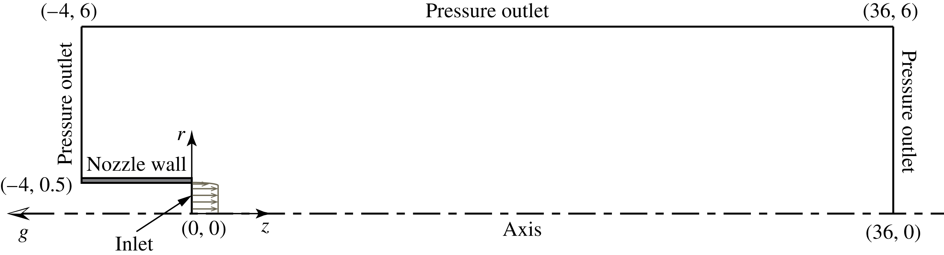
as corresponding eigenvector are obtained by discretizing and solving the EVP (2.15) along with appropriate boundary conditions. Numerical details regarding the base flow computation, and details regarding discretization, boundary conditions and solution of EVP (2.15) are presented in appendix B.
For a global mode, the oscillation frequency and growth/decay rates are given by
 $\unicode[STIX]{x1D714}_{r}$
and
 $\unicode[STIX]{x1D714}_{i}$
respectively. Also, the eigenfunctions namely
 $\hat{v}_{r},\hat{v}_{\unicode[STIX]{x1D703}},\hat{v}_{z},\hat{p},\hat{\unicode[STIX]{x1D70C}}$
represent the possible two-dimensional shape of the perturbations for the corresponding global mode. For a plume base flow, the growth/decay rates
 $\unicode[STIX]{x1D714}_{i}$
of all global modes determine its linear stability. For any global mode, if
 $\unicode[STIX]{x1D714}_{i}>0$
, the plume is said to be globally unstable and it exhibits an oscillatory behaviour, otherwise when
 $\unicode[STIX]{x1D714}_{i}<0$
, it is globally stable. However, in this setting, the convective instabilities (amplifier behaviour) that exist in constant-density jets, and plumes (Chakravarthy et al.
Reference Chakravarthy, Lesshafft and Huerre2015) cannot be predicted, since the perturbations, while growing in amplitude, convect out of the domain in the long time limit and the flow inside the domain remains globally stable. To validate the results obtained from global linear stability analysis, experiments have been carried out.
3 Experimental set-up
Experiments are performed using plumes of helium and helium–air mixtures to validate the results obtained from global linear stability analysis and to address the disparities observed between the results of linear analysis and earlier plume experiments. Flow visualizations, hot-wire measurements and velocity measurements using particle image velocimetry (PIV) are performed to identify the plume instabilities and calculate puffing frequencies. The details of the experimental set-up are as follows.
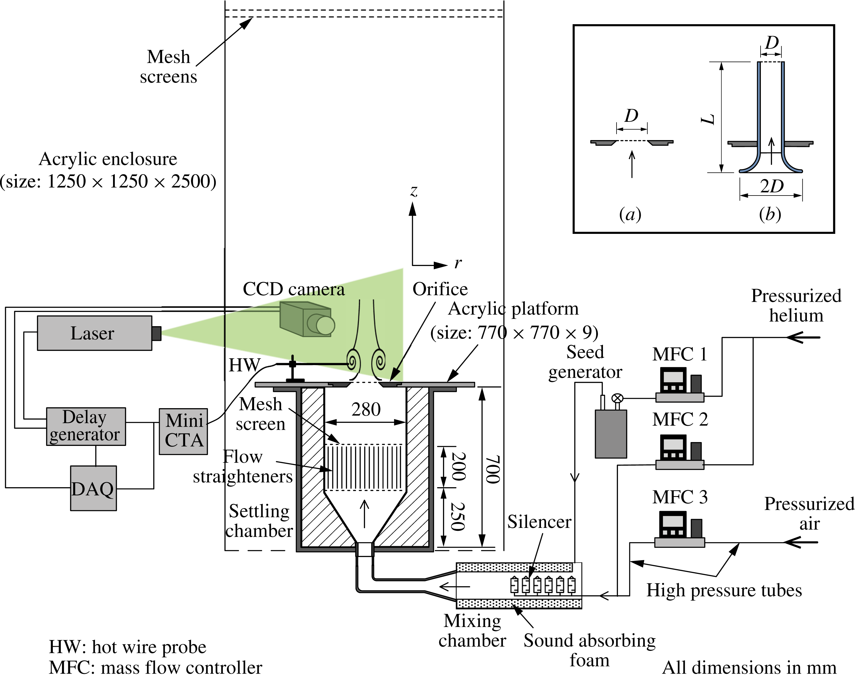
Schematic of experimental set-up. An isolated mixing chamber, a large settling chamber and flow straighteners are salient features to minimize the disturbances. The inset on the right shows the two inlet configurations (a) orifice and (b) pipe nozzle for which the experiments are performed.

The schematic of the experimental set-up is shown in figure 1. The set-up primarily consists of pressurized sources of helium and air, three mass flow controllers, a seed generator, mixing chamber, settling chamber and an orifice/nozzle through which the plume fluid ejects out into the ambient air. Dry gases of helium and air are fed from pressurized tanks to mass flow controllers (Alicat Scientific, MFC-100slpm, MFC-1000slpm and MFC-2000slpm), where the mass flow rates of these gases are monitored and precisely controlled by a feedback mechanism. The mass flow rate proportions of helium and air required to be mixed in order to achieve a desired inlet velocity and density are precalculated, and these values are set using the respective MFCs. A small fraction of helium is bypassed through a seed generator where it is seeded with oil particles. The unseeded helium and air are passed through a series of silencers which open into a mixing chamber. The seeded helium gas later joins the unseeded gas mixture in the mixing chamber and this gas mixture enters the settling chamber at its bottom. In the settling chamber, the gas mixture passes through a diverging section, a flow straighter and a series of mesh screens, and finally ejects out into the ambient air though an orifice/pipe nozzle. The top of the settling chamber is concealed using an acrylic platform which had an opening at its centre for mounting various orifices/pipe nozzles as shown in figure 1. A flat mesh screen is fitted across the exit plane of the orifice/pipe nozzle. The purpose of this screen is to prevent the back flow of heavier ambient air into the settling chamber which is filled with lighter plume fluid and provide a uniform flow condition at the orifice exit. The settling chamber is surrounded by a large cuboid shaped enclosure to prevent the plume from any ambient disturbances. To further prevent the plume from ambient disturbances, two flat mesh screens are sandwiched and placed over the top opening of the cubical enclosure as shown in figure 1.
Note that the set-up built in the present experiments is different from that used in earlier plume experiments of Cetegen & Kasper (Reference Cetegen and Kasper1996) and Cetegen (Reference Cetegen1997). Since the present work investigates the plume instability and transition, the set-up has been designed carefully to minimize the disturbances in the settling chamber and to prevent the plume from unwanted fluctuations/forcing. A distinct feature in the present set-up is the usage of a separate mixing chamber upstream of the settling chamber, which houses a series of silencers (Festo 2316) through which the fluid from MFCs eject out. The purposes of these silencers are multifold. The use of silencers minimizes the acoustic noise that arises when the pressurized gas enters the mixing chamber, damp the pressure fluctuations that arise due to MFC valve oscillations because of automated feedback control, and enhance the mixing between the seeded and unseeded gases by equally dispersing the unseeded gas in all directions. Additionally, the mixing chamber walls are lined using sound absorbing foam to minimize the acoustic noise further that may arise at seeded gas entry. Without mixing chamber, it has been observed that these disturbances/fluctuations enter the settling chamber directly and influence the plume oscillation frequencies, presumably by inducing some forcing, particularly for larger source diameters and flow rates. Further, in the settling chamber, the flow straightener and mesh screens breakdown the larger eddies and ensure a more uniform flow upstream of the plume source.
In the present work, plumes emanating from orifices are investigated extensively. Since the earlier experiments of Cetegen & Kasper (Reference Cetegen and Kasper1996) and Cetegen (Reference Cetegen1997) investigated plumes ejecting from pipe nozzles, fewer experiments have been performed for plumes emanating from pipe nozzles in order to compare with earlier experiments and investigate the effect of change in plume source conditions on plume transition and puffing. The schematics of these two inlet configurations are shown in the inset of figure 1. The pipe nozzles are fabricated with a bell mouth shaped inlet for smoother entry of plume fluid. The dimensions of various orifices and pipe nozzles used in the present work are listed in table 1.
Plume inlet configurations and their dimensions. The value in brackets for each pipe nozzle shows the corresponding length to diameter ratio
 $L/D$
.

The velocity field in plumes is measured in a time resolved manner using a PIV system, which consists of a dual cavity Nd:YAG laser (
 $100~\text{mJ}~\text{pulse}^{-1}$
, 50 Hz) for illumination, a 10 bit CMOS camera (
 $2336\times 1728$
pixels resolution) for capturing the particle images and a programmable pulse sequences generator (Sequencer V801-BM) for synchronizing the laser and camera. Two oil particle based seed generators, developed in-house, are used for seeding the flow field. The first one, connected to MFC1 as in figure 1, is used to seed the plume fluid. The seeding concentration levels in the plume fluid can be controlled by adjusting the helium flow rate in MFC1 and diverting the remaining helium through MFC2. Prior to each experimental run, the air in the cubical enclosure is seeded using a second seed generator (not shown here) in order to capture the velocity field of the ambient air entrained by the plume. High pressure air (from an air compressor) is used to generate seeding from the second seed generator. Edible soya-bean oil is used as working fluid in both the seed generators that generate oil particles of size
 ${\approx}2{-}3~\unicode[STIX]{x03BC}\text{m}$
. The time between the two laser pulses is optimized such that the particle displacement is approximately 25–30 % of the interrogation window. To obtain the velocity fields from image pairs, the PIV analysis is carried out using a multigrid cross-correlation algorithm with window deformation (Scarano & Riethmuller Reference Scarano and Riethmuller2000). The spurious vectors are detected using universal outlier detection (Westerweel & Scarano Reference Westerweel and Scarano2005) and are replaced by interpolating vectors from neighbouring cells.
The flow field involves high velocity gradients due to buoyant acceleration. Therefore, for the seed particles to follow the plume fluid faithfully, the particle response time should be less than the smallest time scale of the plume. The particle Stokes number (
 $St_{k}$
), the ratio of particle relaxation time
 $\unicode[STIX]{x1D70F}_{p}$
(response time constant of a particle) to the characteristic time scale of flow
 $\unicode[STIX]{x1D70F}_{f}$
, gives an estimate of how strictly the seed particles follow the fluid flow and respond to high velocity gradients. The particle relaxation time is given by Melling (Reference Melling1997) as
 $\unicode[STIX]{x1D70F}_{p}=\unicode[STIX]{x1D70C}_{p}d_{p}^{2}/18\unicode[STIX]{x1D707}$
, where
 $\unicode[STIX]{x1D70C}_{p}$
and
 $d_{p}$
are the particle density and diameter respectively, and
 $\unicode[STIX]{x1D707}$
is the fluid viscosity. The characteristic flow time scale
 $\unicode[STIX]{x1D70F}_{f}=D/V_{0}$
is estimated from inlet diameter and velocity. The Stokes number thus calculated for the smallest possible flow time scale is
 $St_{k}=2.5\times 10^{-4}$
, which is much less than 1, implying that the tracer particles faithfully follow the plume fluid. The uncertainty in the velocity obtained using PIV is mainly because of four sources i.e. equipment (calibration and timing), particle lag, sampling size and processing algorithm (Lazar et al.
Reference Lazar, Deblauw, Glumac, Dutton and Elliott2010). By considering these sources of errors, the maximum error in velocity is found to be within
 $\pm 1.8\,\%$
of characteristic velocity. The obtained velocity fields in puffing plumes are used to calculate puffing frequencies. Also, the velocity field obtained in steady laminar plumes are used to validate the base flow solution. The seed particle images are used as flow visualizations to observe plume instabilities.
A hot-wire probe is placed normal to streamwise direction near the orifice/nozzle lip, at
 $(r,z)=(0.5,0.5)$
(axes shown in figure 1 with its origin at the centre of plume source). For each case, the voltage signal from the hot-wire is acquired at 2000 Hz for 20 s using a NI 4472, 24-bit DAQ card. The hot-wire signal and the flow visualizations are used to characterize the plume state i.e. non-puffing or puffing. Also, the voltage trace from the hot-wire is used to calculate puffing frequency.
4 Results and discussion
4.1 Base flow field
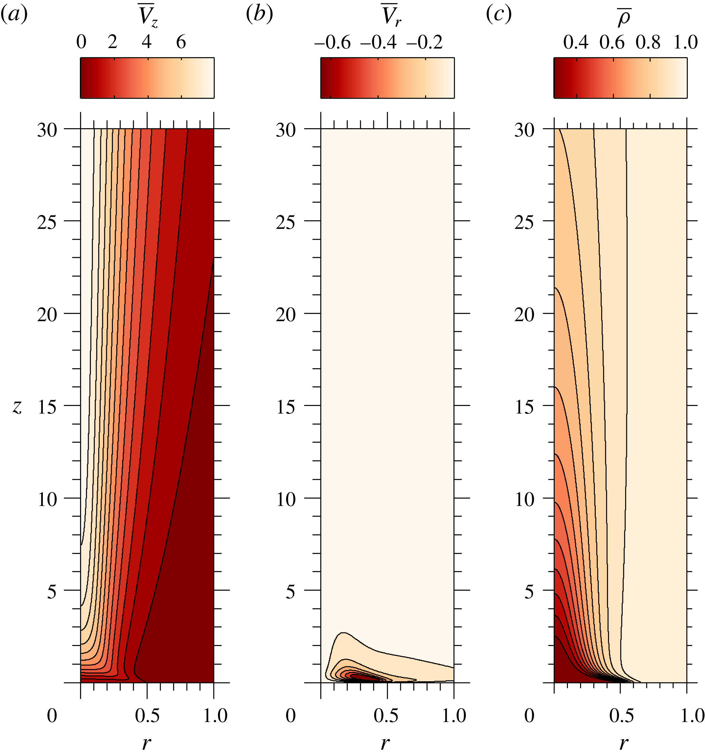
To understand the nature of the base flow, a representative flow field of a laminar buoyant plume is presented in figure 2, which shows the axial and radial velocity fields along with the density field for
 $Re=100$
,
 $Fr=0.5$
and
 $S=0.276$
. Figures 3(a) and 3(b) show the corresponding centreline velocity and mass-fraction variations respectively, along with two other
 $Fr$
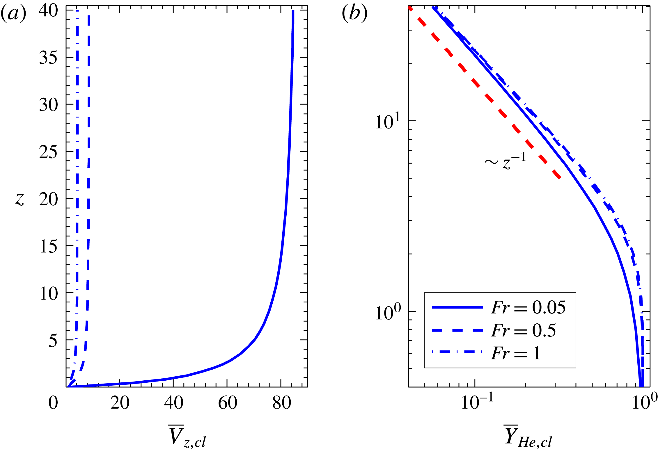
, 0.05 and 1. Lighter plume fluid ejecting from the inlet accelerates continuously due to buoyancy and the velocity rapidly increases along the centreline. Due to this rapid acceleration, the plume envelop converges radially towards the centreline, which is accompanied by a dominant radial inflow near the plume inlet as shown in figure 2(b). As the plume fluid convects downstream, it gets diluted as seen from the density field in figure 2(c) due to effects of mass diffusion, and the viscous diffusion results in the entrainment of the ambient fluid. Further downstream, the acceleration effects of buoyancy are balanced by deceleration effects of entrainment (Gebhart et al.
Reference Gebhart, Jaluria, Mahajan and Sammakia1988) and therefore, the centreline velocity asymptotically reaches a constant value with increase in height, as shown in figure 3(a), thereby attaining self-similarity. In this self-similar region, the helium mass fraction along the centreline achieves a power-law decay as
 $z^{-1}$
, as shown in figure 3(b), consistent with the laminar buoyant plume theory (Gebhart et al.
Reference Gebhart, Jaluria, Mahajan and Sammakia1988).
(a) Axial velocity, (b) radial velocity and (c) density fields in a laminar buoyant plume of
 $Re=100$
,
 $Fr=0.5$
and
 $S=0.276$
obtained from steady base flow computations.

(a) Velocity and (b) helium mass-fraction variations along the axis for different Froude number buoyant plumes at
 $Re=100$
and
 $S=0.276$
. The plots show that plumes attain self-similarity in the far field i.e.
 $\overline{V}_{z,cl}\sim$
constant and
 $\overline{Y}_{He,cl}\sim z^{-1}$
.

4.2 Instability analysis
In this section, the results obtained from global linear stability analysis are presented in the
 $Re{-}Fr{-}S$
parameter space. The density ratio
 $S$
has been varied in the range
 $0.138\leqslant S\leqslant 0.967$
, i.e. the plume inlet density varied from pure helium density to 97 % of air density by changing the inlet helium mass fraction,
 $Y_{He0}$
from 1 to 0.0055. For a fixed density ratio,
 $Re$
and
 $Fr$
are varied in ranges
 $20\leqslant Re\leqslant 1000$
and
 $0.01\leqslant Fr\leqslant 1$
respectively. In the density ratio range investigated, the remaining two non-dimensional parameters, i.e. the viscosity ratio
 $\unicode[STIX]{x1D707}^{\ast }$
and the Schmidt number
 $Sc$
exhibit a minor variation in ranges of 1–1.1 and 1.6–1.7 respectively. Since these variations in
 $\unicode[STIX]{x1D707}^{\ast }$
and
 $Sc$
are smaller when compared to other parameters, we have not looked into the effects of these two parameters in the present work.
The eigenvalues and corresponding two-dimensional eigenfunctions are calculated at each discrete parameter set (
 $Re$
,
 $Fr$
and
 $S$
) for azimuthal wavenumbers
 $m=0$
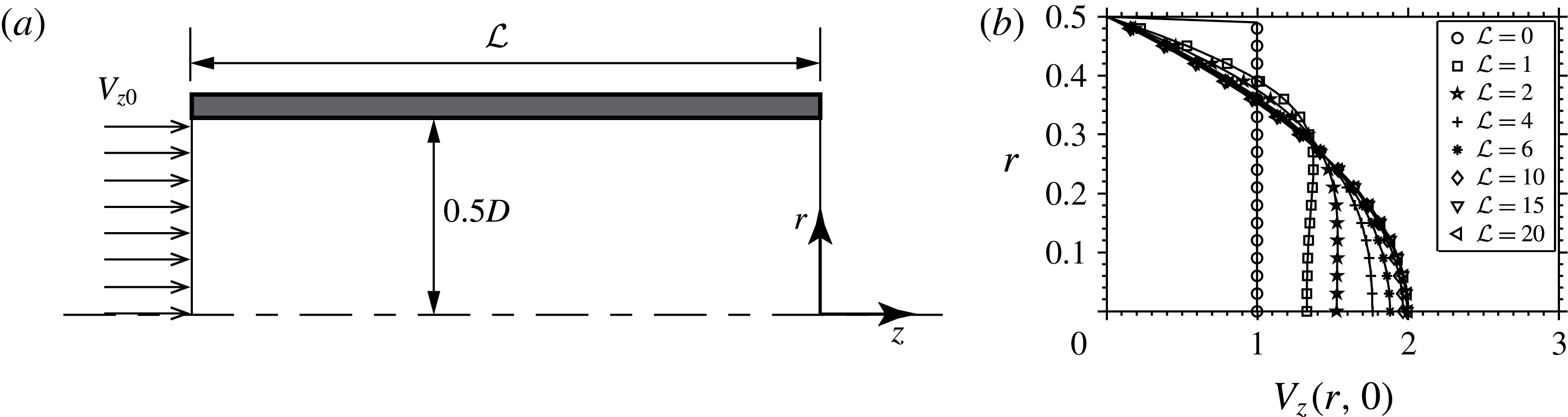
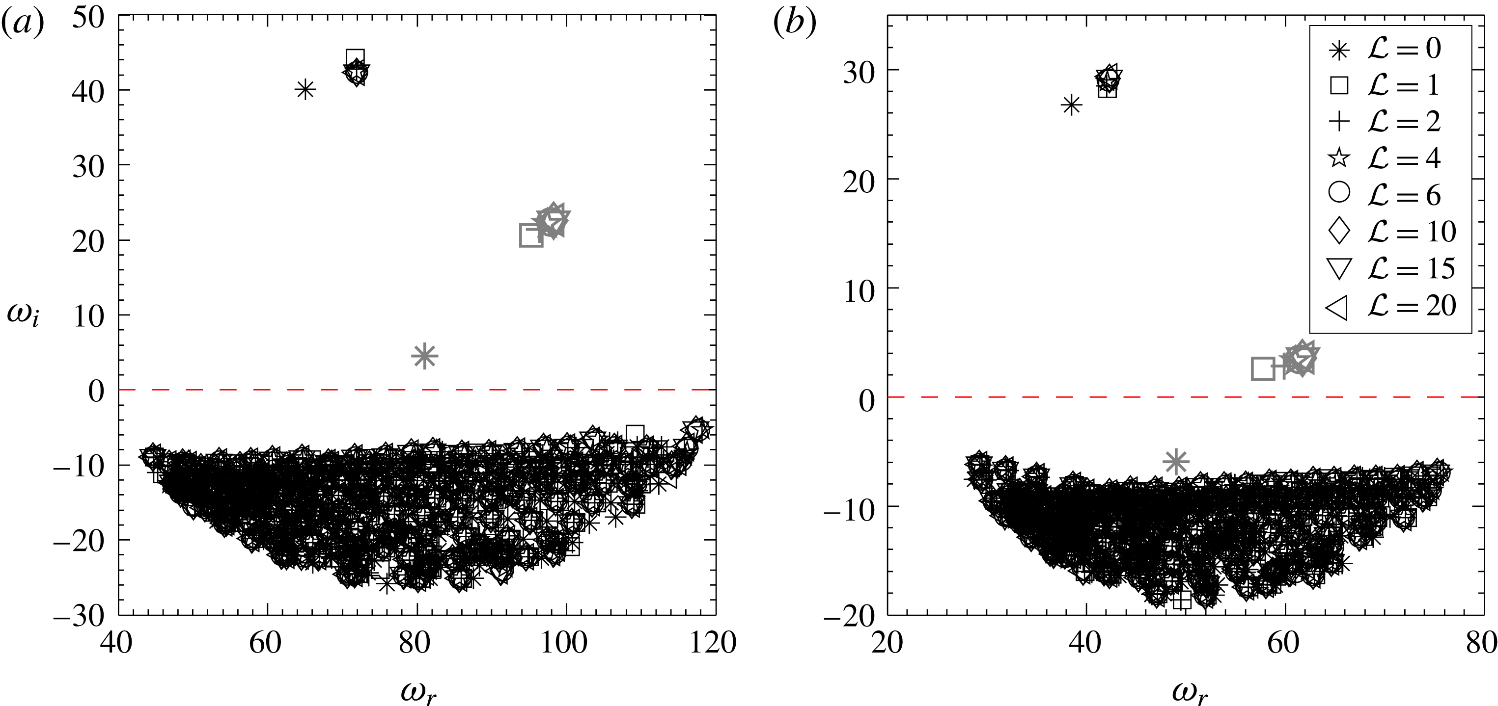
, 1 and 2. Unless specified, both velocity and density profile steepness parameters in (B 1) and (B 2) respectively, are set to 100 in all the calculations in order to simulate plumes with near uniform (top-hat) inlet velocity and mass-fraction profiles. Nevertheless, the effect of the change in velocity profile on plume instability characteristics is also investigated and will be discussed later in § 4.4.
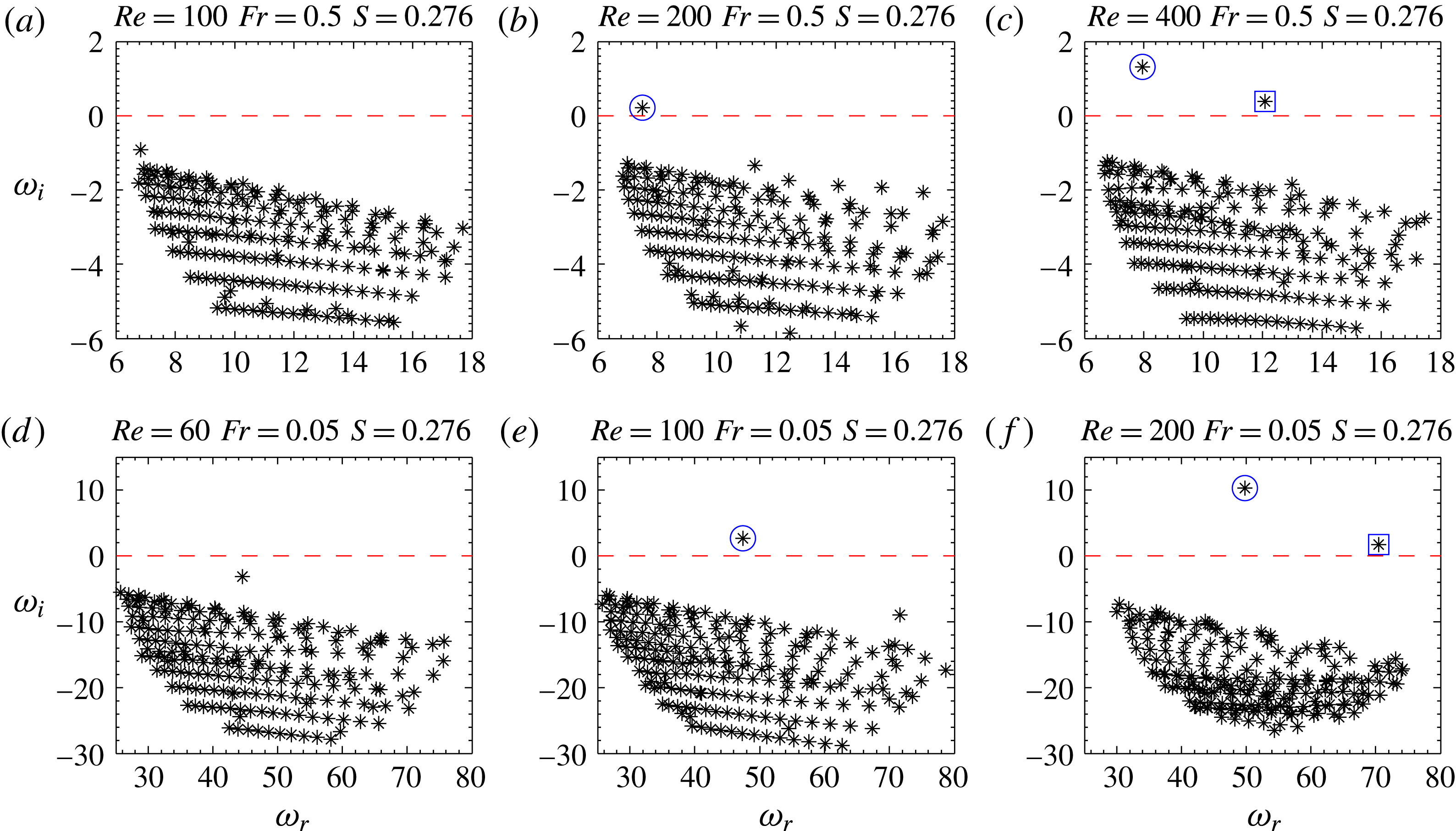
Eigenvalue spectrum with increase in
 $Re$
at fixed density ratio, and at Froude numbers (a)–(c)
 $Fr=0.5$
and (d)–(f)
 $Fr=0.05$
. The eigenvalues marked in ○ and ▫ correspond to primary and secondary modes respectively.

4.2.1 Instability modes
The eigenvalue spectra obtained for axisymmetric perturbations
 $m=0$
are presented in figure 4, for two Froude numbers 0.5 (4
a–c) and 0.05 (4
d–f) and density ratio
 $S=0.276$
. At each
 $Fr$
, the evolution of eigenvalue spectrum with increase in
 $Re$
is also presented to identify the unstable modes.
For a fixed
 $Fr$
and
 $S$
, at low
 $Re$
, the calculations indicate that the flow is stable for
 $m=0$
with all eigenvalues lying in the stable half-plane (see 4
a,d). With an increase in
 $Re$
, the flow becomes unstable, with a single eigenvalue moving into the unstable half-plane as shown in 4(b,e). This eigenvalue, highlighted in circle in figure 4(b–f), will be referred as ‘primary mode’ hereafter. With further increase in
 $Re$
, a second eigenvalue moves into the unstable half-plane which is highlighted in square in 4(c,f). This eigenvalue will be referred to as the ‘secondary mode’ hereafter. Eigenvalue spectra in the entire parameter space considered in this study for higher azimuthal modes
 $m=1$
and 2 do not contain any discrete unstable eigenvalues. Therefore, the buoyant plumes are globally unstable only for
 $m=0$
, and are globally stable for
 $m=1$
and 2, in the parameter range considered in the present study. An experimental investigation of circular plumes of helium and helium–air mixtures by Cetegen & Kasper (Reference Cetegen and Kasper1996) and Cetegen (Reference Cetegen1997), and in buoyant hot gas plumes and pool fires by Cetegen & Ahmed (Reference Cetegen and Ahmed1993) showed that their near-field instability is characterized by self-sustained oscillations, which involves periodic shedding of vortices that are axisymmetric in nature. In these experiments and in the present experiments (which are discussed in § 4.3), the oscillatory instabilities observed are axisymmetric and no asymmetric instabilities are observed in the near field. Similarly, Chakravarthy (Reference Chakravarthy2015) investigated the global stability of buoyant hot jets and thermal plumes and found only
 $m=0$
to be globally unstable, and
 $m=1$
to be stable. While the buoyant jets and thermal plumes in their study exhibited only one unstable global mode, plumes of helium and helium–air mixtures exhibited two such modes. The most unstable mode in their global eigenvalue spectra corresponds to the primary mode of the present study. Since plumes remain stable to higher azimuthal perturbations, we confine our further discussion to axisymmetric perturbations (
 $m=0$
) and investigate the variation of dimensionless oscillation frequencies i.e. Strouhal number
 $St=\unicode[STIX]{x1D714}_{r}/2\unicode[STIX]{x03C0}$
and growth rates
 $\unicode[STIX]{x1D714}_{i}$
of primary and secondary modes for different parameter values.
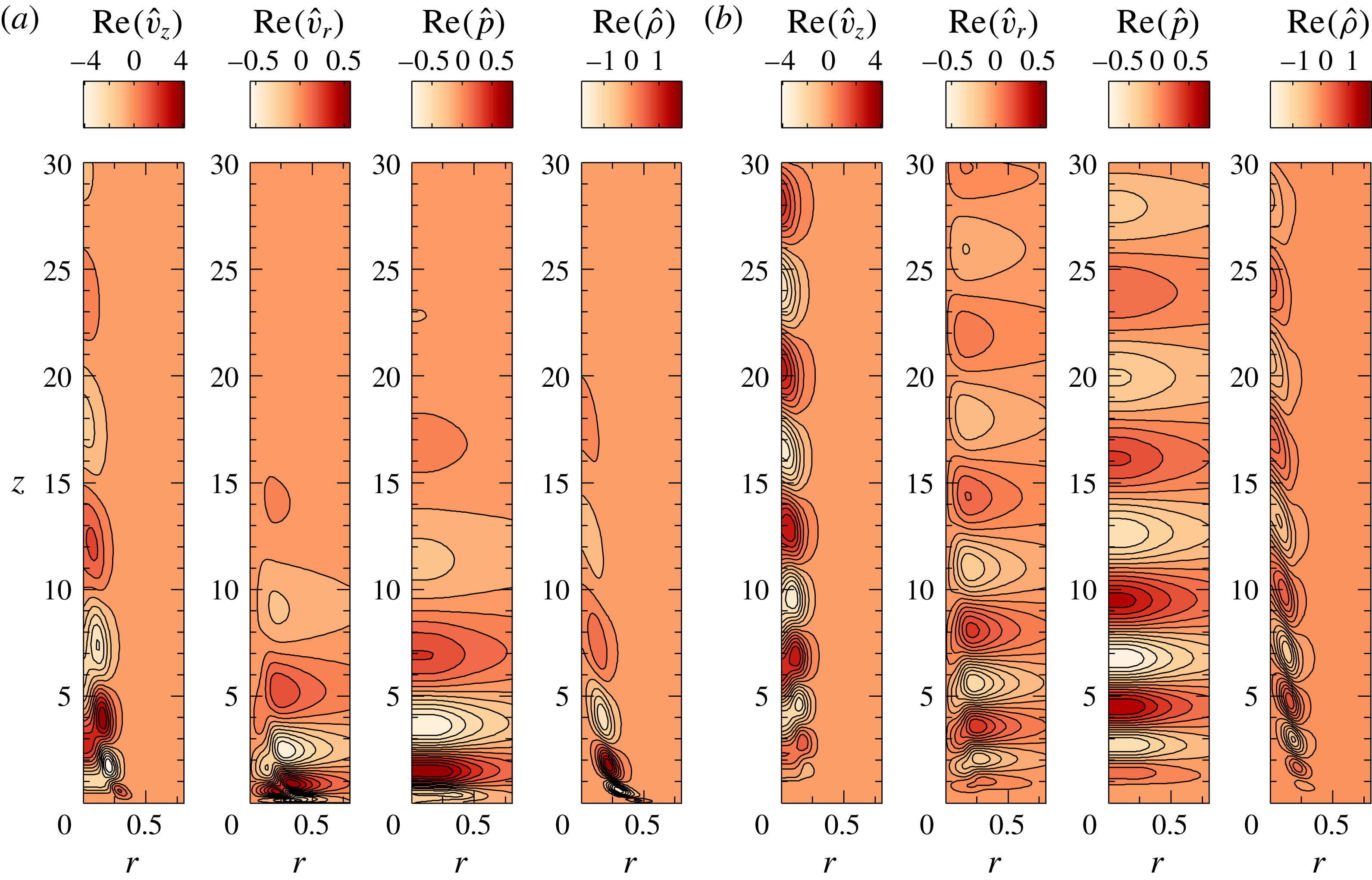
Eigenfunctions of (a) primary and (b) secondary modes for
 $Re=400$
,
 $Fr=0.5$
and
 $S=0.276$
. These eigenfunctions are scaled by 100 and normalized using
 $\Vert \hat{q}\Vert$
.

The real part of the eigenfunctions corresponding to the primary and secondary modes for the case
 $Re=400$
,
 $Fr=0.5$
and
 $S=0.276$
(corresponding to figure 4
c), are shown in figures 5(a) and 5(b) respectively. The eigenfunctions of both these modes show spatially periodic structures, which are a characteristic of an oscillatory instability. The imaginary part of the eigenfunctions (not shown here) are similar to their real counterparts but are in spatial quadrature, with the zeros of the imaginary parts located approximately at the extrema of their real parts. This phase shift implies that these structures convect downstream as they grow. The shape of eigenfunctions of both primary and secondary modes are qualitatively similar. However, the maximum amplitude of the primary mode always lies closer to the inlet than that of the secondary mode. Structures observed in the contours of secondary mode eigenfunctions extend further downstream when compared to that of the primary mode. Near the exit of the plume source, the density fluctuations are confined to the region of the maximum density gradient and become negligible in the vicinity of the plume axis, while the axial velocity and pressure fluctuations are also significant near the plume axis. It is also observed that, with an increase in
 $Re$
, the location of maximum amplitude of all perturbations shifts upstream closer to the plume source (not shown here for brevity).
4.2.2 Effect of
 $Re$
,
$Fr$
and
$S$
on oscillation frequency and growth rates


The effect of
 $Re$
,
 $Fr$
and
 $S$
on the dimensionless oscillation frequency,
 $St$
and growth rate,
 $\unicode[STIX]{x1D714}_{i}$
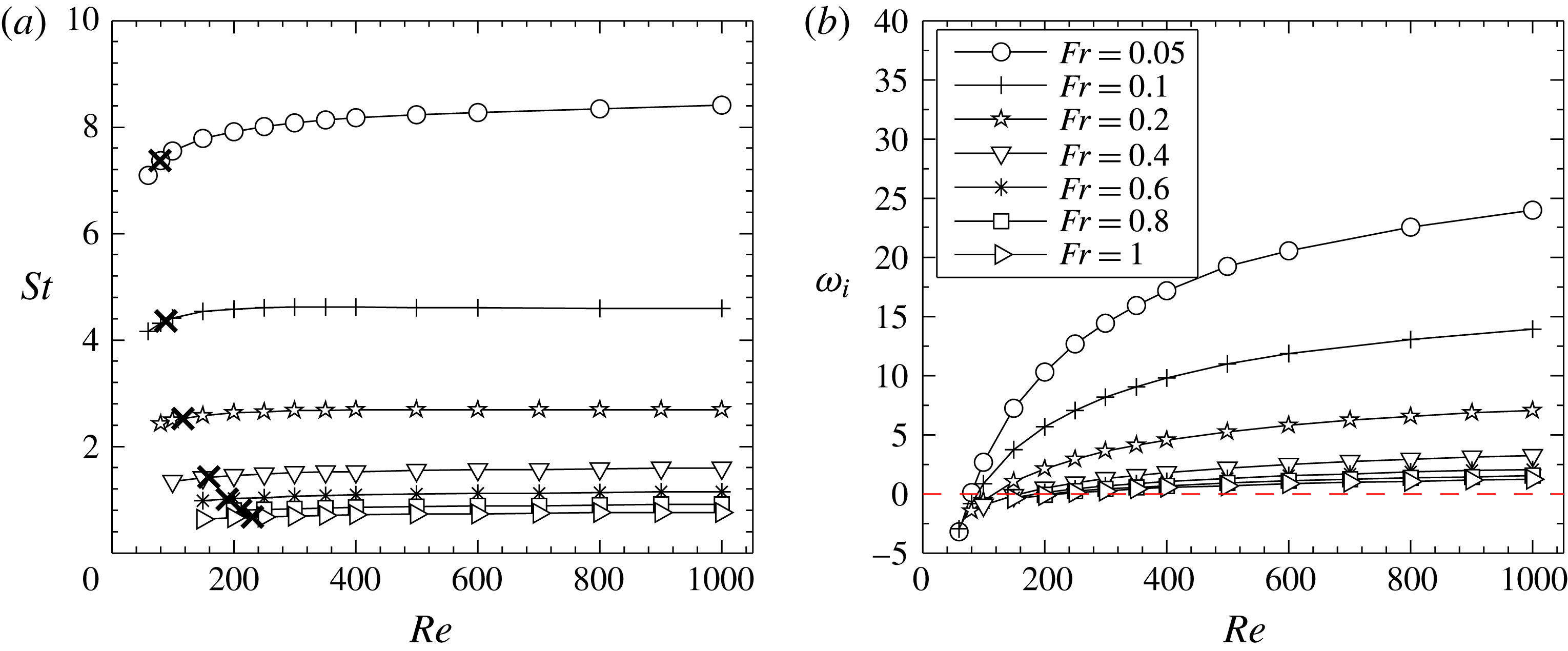
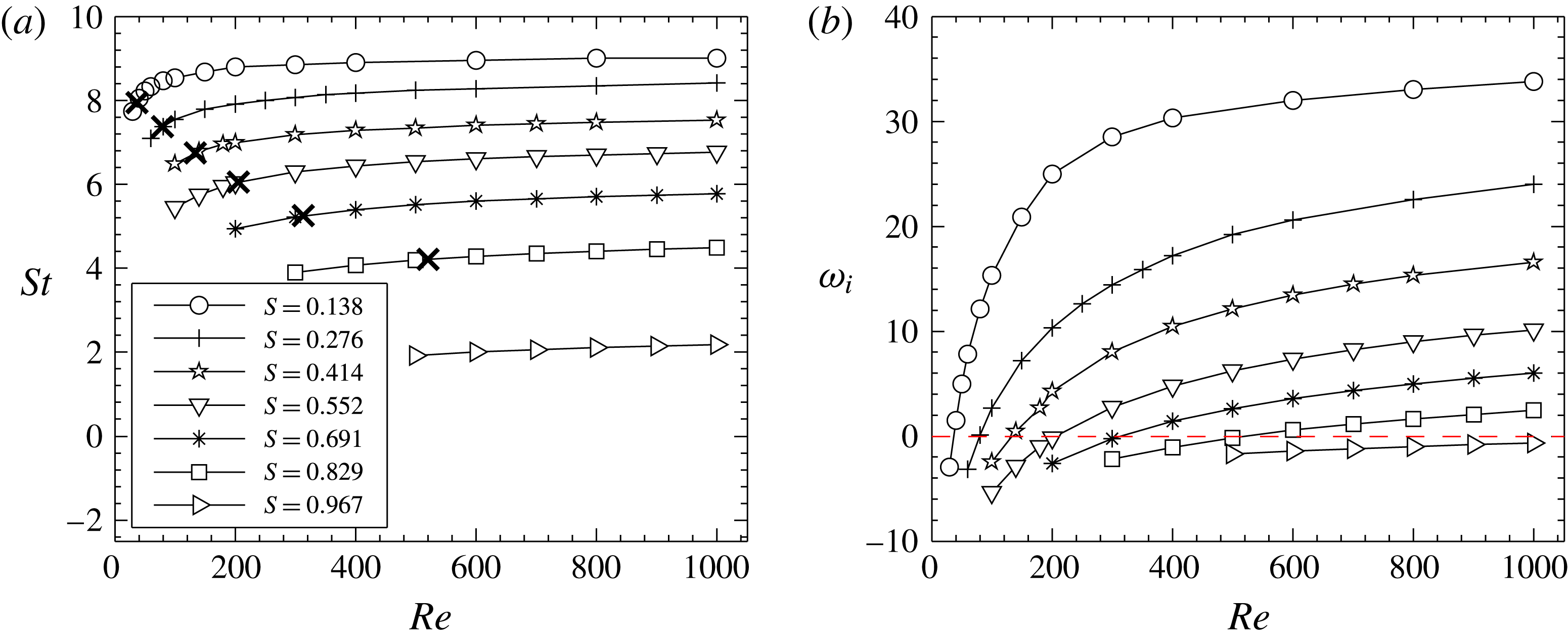
of the primary mode is considered in order to investigate the relative importance of these non-dimensional parameters on plume instability. The variation of
 $St$
with
 $Re$
, plotted for different
 $Fr$
and
 $S$
in figures 6(a) and 7(a) respectively, reveals that
 $Fr$
and
 $S$
are the important parameters that govern the plume oscillation frequencies, while the effect of
 $Re$
is relatively insignificant. For a fixed
 $Fr$
and
 $S$
,
 $St$
exhibits a weaker dependence on
 $Re$
near the transition point, which diminishes with a further increase in
 $Re$
. This relative independence of
 $St$
on
 $Re$
shows that viscous diffusion has a negligible impact on plume oscillation frequencies. The stronger dependence of
 $St$
on
 $Fr$
and
 $S$
shows that the plume oscillations are largely impacted by gravity and density difference (between source and ambient) through buoyancy. Further, it can be observed from figure 6(a) that, the dependence of
 $St$
on
 $Fr$
gradually diminishes with an increase in
 $Fr$
. This implies that, for a fixed plume density, with a decrease in buoyancy or increase in inertial forces i.e. as the buoyant plumes approach buoyant jet regime, the oscillation frequencies tend to become independent of
 $Fr$
. This is consistent with an earlier work in buoyant jets in the
 $Fr$
range 2-
 $\infty$
by Nichols et al. (Reference Nichols, Schmid and Riley2007), who found that
 $St$
in buoyant jets is least impacted by
 $Fr$
and only depends on
 $S$
. The reason for this difference in
 $St$
dependence between buoyant jets and plumes will be qualitatively assessed later in § 4.5, where the instability mechanism responsible for these oscillations is investigated using the vorticity transport equation.
Variation of (a)
 $St$
and (b)
 $\unicode[STIX]{x1D714}_{i}$
of the primary mode with
 $Re$
for different
 $Fr$
, at a fixed
 $S=0.276$
.
 $\boldsymbol{\times }$
corresponds to critical
 $Re$
at which the plumes become unstable.

Variation of (a)
 $St$
and (b)
 $\unicode[STIX]{x1D714}_{i}$
of the primary mode with
 $Re$
for different
 $S$
, at a fixed
 $Fr=0.05$
.
 $\boldsymbol{\times }$
corresponds to critical
 $Re$
at which the plumes become unstable.

The corresponding growth rate variations plotted in figures 6(b) and 7(b) show that plume growth rates are dependent on all these three non-dimensional parameters. Although the viscous forces have a negligible impact on
 $St$
, variation of
 $\unicode[STIX]{x1D714}_{i}$
with
 $Re$
shows that they play a dominant role in the growth of the instability. For a fixed
 $Fr$
and
 $S$
, the lower growth rates at low
 $Re$
imply that viscous forces act to damp the plume oscillations and stabilize the plumes. With an increase in
 $Re$
, the inertial forces overcome the viscous diffusion and thereby, the intensity of plume oscillations increases, leading to an increase in
 $\unicode[STIX]{x1D714}_{i}$
. Figures 6(b) and 7(b) also show that plumes with lower
 $Fr$
and lower
 $S$
attain higher
 $\unicode[STIX]{x1D714}_{i}$
i.e. the intensity of plume oscillations is higher for plumes of larger buoyancy. Similar to
 $St$
, the dependence of
 $\unicode[STIX]{x1D714}_{i}$
on
 $Fr$
tend to diminish with an increase in
 $Fr$
as observed in figure 6(b), consistent with the growth rate variation in buoyant jets as reported by Nichols et al. (Reference Nichols, Schmid and Riley2007). The trends observed in growth rate variations will be discussed further in § 4.5 in the light of the instability mechanisms responsible for this global instability.
4.2.3 Transition diagrams and frequency scaling
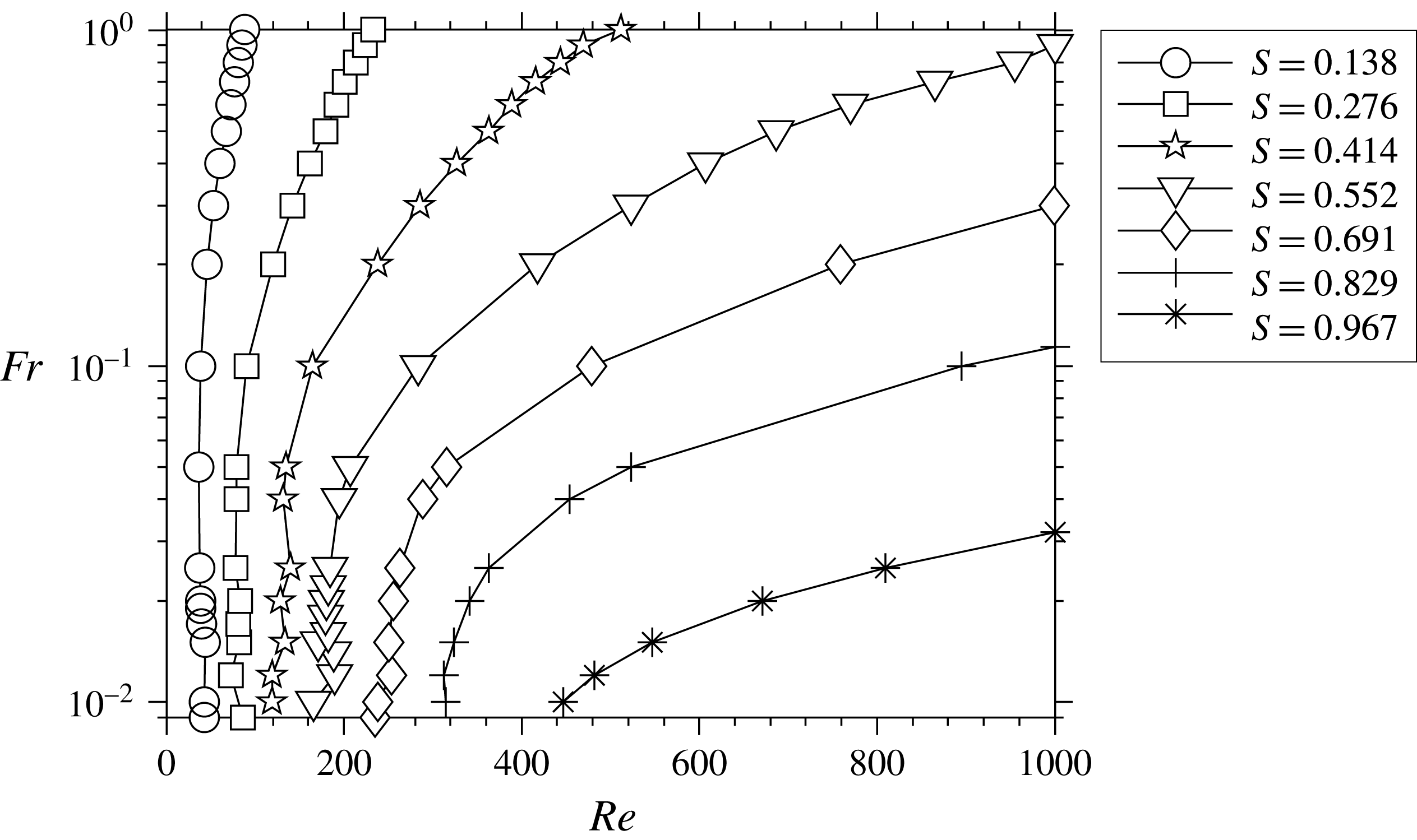
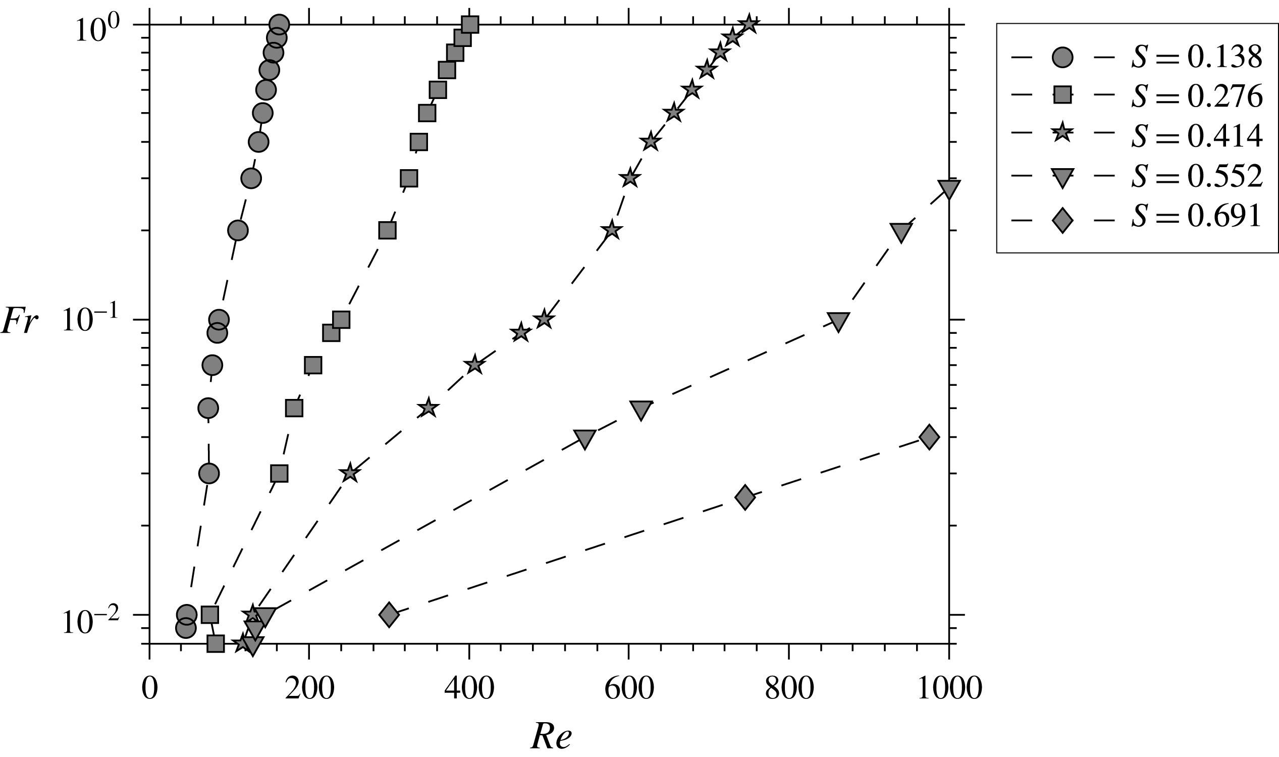
Figure 8 shows the neutral curves obtained for the primary mode. These curves correspond to the contour lines of
 $\unicode[STIX]{x1D714}_{i}=0$
mapped in the
 $Re{-}Fr$
plane, for each
 $S$
. These neutral stability curves reflect the growth rate trends observed in figures 6(b) and 7(b). The critical
 $Re$
is a function of both
 $Fr$
and
 $S$
. For a fixed
 $S$
, the critical
 $Re$
decreases with a decrease in
 $Fr$
, and similarly, for a fixed
 $Fr$
, it decreases with a decrease in
 $S$
. This implies that plumes with larger buoyancy destabilize earlier at lower
 $Re$
. The plume fluid in low
 $Fr$
plumes accelerates heavily in the immediate downstream of the plume source because of higher buoyancy when compared to high
 $Fr$
plumes, as observed in figure 3(a). This leads to a local increase in
 $Re$
and thereby, an earlier destabilization of low
 $Fr$
plumes.
From the above discussion, it is clear that the degree of buoyancy governs the plume transition. An increase in
 $S$
leads to a reduction in buoyancy. Therefore, with an increase in
 $S$
, i.e. as the plume density approaches air density, the unstable region is confined to lower
 $Fr$
(refer figure 8) where the effects of buoyancy are still dominant. In the limit of
 $S\rightarrow 1$
(vanishing density difference), the unstable region vanishes and plumes tend to become globally stable for
 $S=1$
. This has been verified by evaluating the global eigenvalue spectrum for several homogeneous plumes of
 $S=1$
where all the global modes remain stable, which is also consistent with the observation of Garnaud et al. (Reference Garnaud, Lesshafft, Schmid and Huerre2013).
Neutral curves of primary mode in
 $Re$
–
 $Fr$
plane for various
 $S$
.

Neutral curves of secondary mode in
 $Re$
–
 $Fr$
plane for various
 $S$
.

Using experiments on helium and helium–air mixtures emanating into air, Cetegen (Reference Cetegen1997) mapped the region of instability in the
 $Re{-}S$
plane by neglecting the effect of
 $Fr$
and observed that these oscillating instabilities only occur below a critical density ratio
 $S$
in range 0.5–0.6. Beyond this critical density ratio, they observed the plume to become convectively unstable with Kelvin–Helmholtz instabilities similar to the case of a homogeneous jet. However, the present global stability analysis reveals that these oscillatory instabilities exist even at density ratios higher than the critical density ratio reported by Cetegen (Reference Cetegen1997), for example at
 $S=0.691$
, 0.829 and 0.967. Also, the present work shows that
 $Fr$
has a significant effect on plume transition, particularly at higher
 $S$
and hence, its effect should not be ignored. With these observations deduced for the primary mode, we investigated the plume instability further by looking into the nature of the other unstable global mode i.e. the secondary mode (see figure 4
c,f).
Variation of growth rates of primary and secondary modes with
 $Fr$
for various
 $Re$
and fixed
 $S=0.552$
. The graphs show switching of instability from primary to secondary mode as
 $Re$
and
 $Fr$
are decreased.

 $St$
and
 $\unicode[STIX]{x1D714}_{i}$
of the secondary mode exhibit variations similar to those of the primary mode. The neutral curves for the secondary mode, plotted in figure 9, show that its critical
 $Re$
is always higher than that of the primary mode. The primary mode exhibits higher growth rates than the secondary mode for most of the parameter space investigated except for plumes of very low
 $Fr$
(i.e.
 $O(10^{-3}{-}10^{-2})$
) and at low
 $Re$
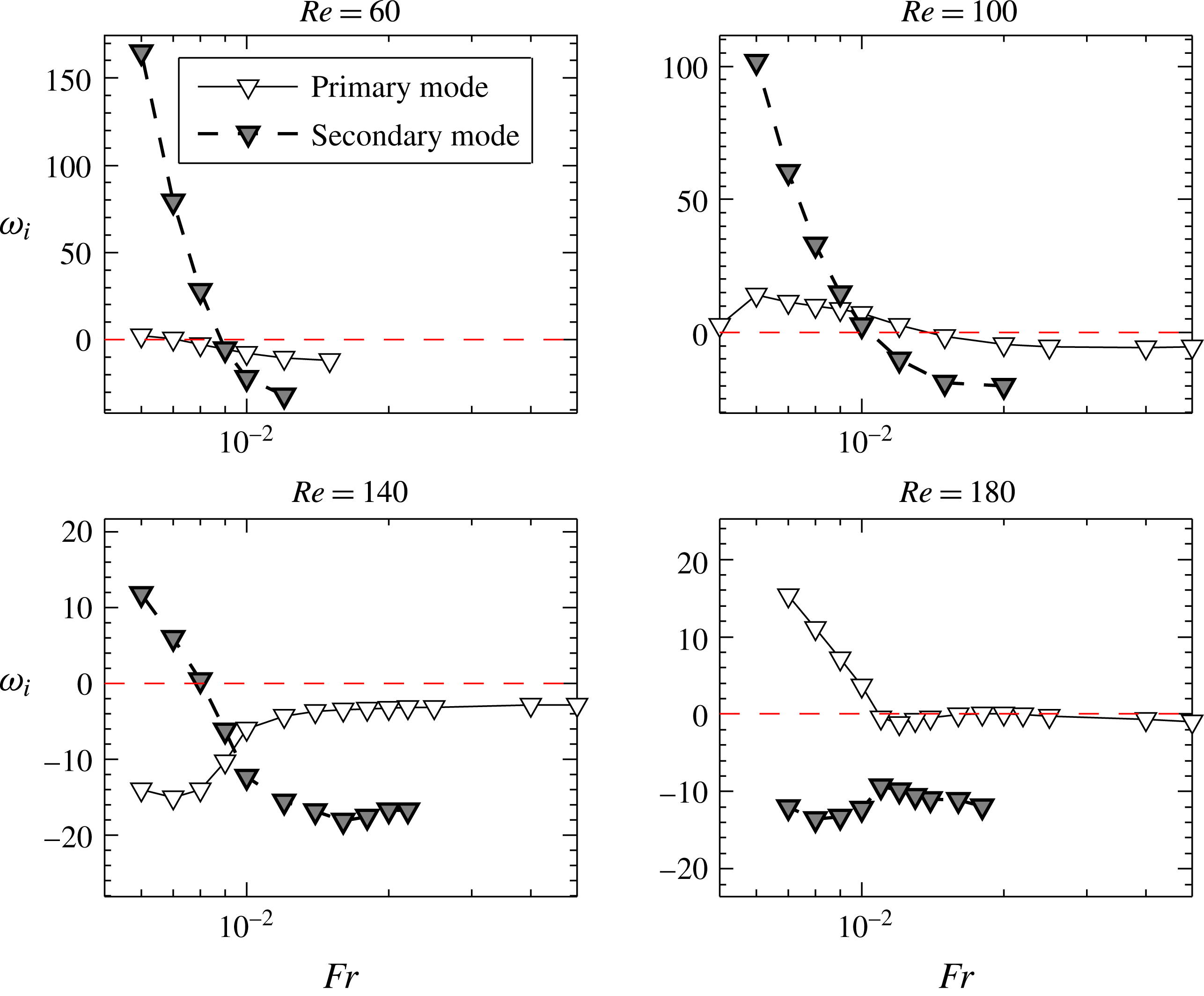
i.e. plumes with very high buoyancy. This mode switching can be illustrated better using figure 10 which compares the variation of growth rates
 $\unicode[STIX]{x1D714}_{i}$
of primary and secondary modes with
 $Fr$
, at four different
 $Re$
and a fixed density ratio
 $S=0.552$
. For
 $Re=60$
, 100 and 140, the secondary mode dominates the primary mode below a
 $Fr\approx 0.009$
(see figure 10), while for
 $Re=$
180, the primary mode becomes dominant at all
 $Fr$
. The
 $Re$
and
 $Ri$
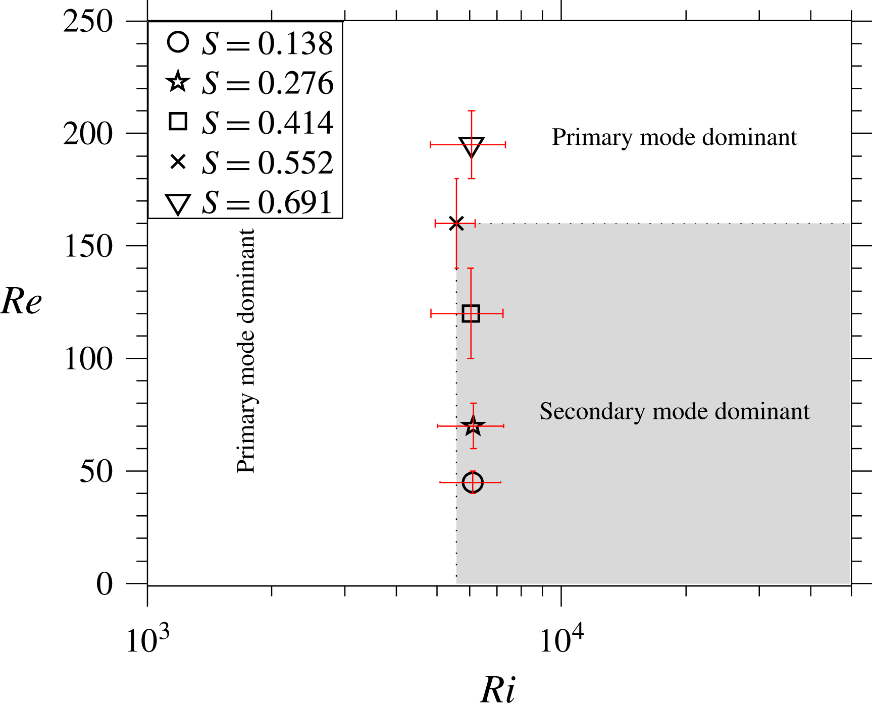
ranges in which this mode switching occurs has been identified for different
 $S$
, and plotted in figure 11. The variations denote the ranges of
 $Re$
and
 $Ri$
in which the mode switching can occur. With an increase in plume density ratio, the
 $Re$
at which mode switching occurs (denoted by
 $Re_{ps}$
hereafter) increases, whereas the corresponding
 $Ri$
ranges remain relatively constant with
 $S$
(refer figure 11). The average
 $Ri$
at which switching occurs for various
 $S$
is found to be
 $Ri\approx 6000$
. Thus, the secondary mode becomes dominant only in the domain
 $Ri>6000$
and
 $Re<Re_{ps}$
. As an example, for
 $S=0.552$
, the shaded region shown in figure 1 will have a dominant secondary mode. This region will reduce substantially for S=0.138, where
 $Re_{ps}\approx 45$
. Note that for plumes of
 $Ri<6000$
, it is the primary mode that dominates irrespective of
 $Re$
.
 $Re{-}Ri$
plane showing the domain in which secondary mode becomes dominant. This domain depends on density ratio. As an example, the domain for
 $S=0.552$
where secondary mode dominates is shown as shaded area. The dominant mode switches from primary to secondary at
 $Ri\approx 6000$
and at an
 $Re$
that depend on
 $S$
.

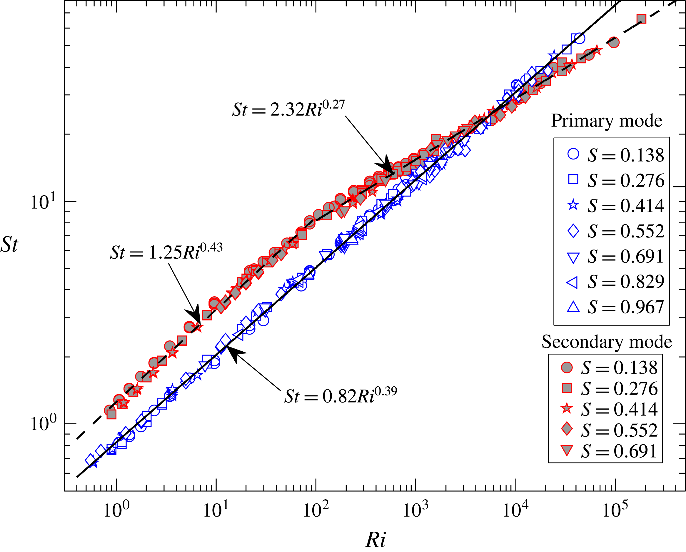
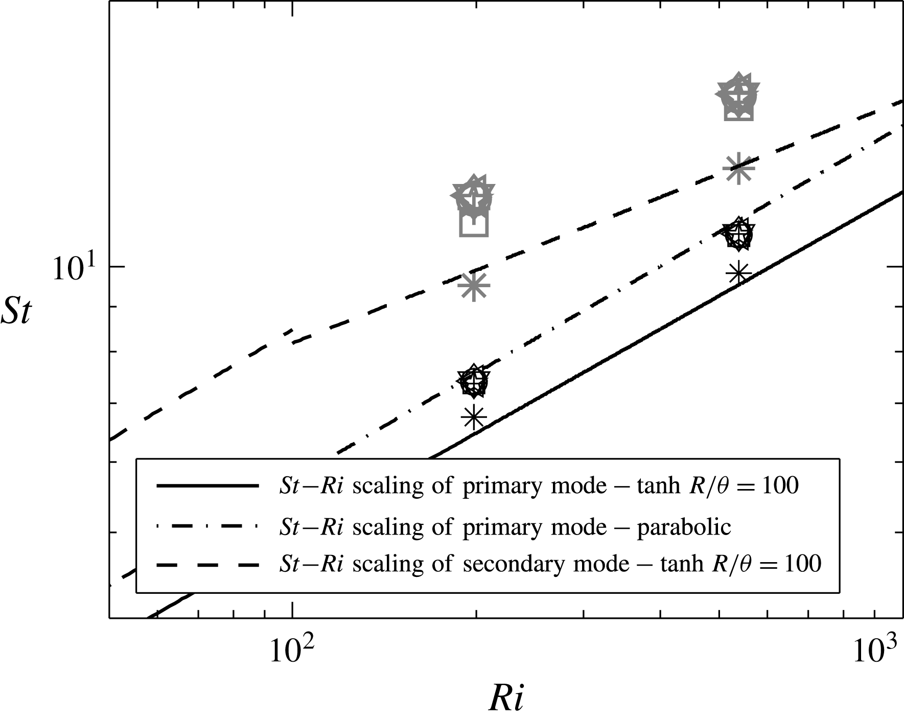
The Strouhal numbers of all the unstable primary and secondary modes are plotted as a function of their Richardson numbers in figure 12. The dependence of oscillation frequencies of both primary and secondary modes on various inlet parameters are well scaled by
 $St{-}Ri$
correlations, similar to experimental observation of (Cetegen & Kasper Reference Cetegen and Kasper1996). The power-law scaling of
 $St$
with
 $Ri$
, obtained for primary and secondary modes in the present study, are shown in figure 12. While the Strouhal number of the primary mode follows a single power law
 $St=0.82Ri^{0.39}$
, the secondary mode follows two power-law fits depending on
 $Ri$
. For
 $Ri<100$
, the Strouhal number of secondary mode varies as
 $St=1.25Ri^{0.43}$
and for
 $Ri>100$
, it varies as
 $St=2.32Ri^{0.27}$
. In the plume experiments, Cetegen & Kasper (Reference Cetegen and Kasper1996) observed two
 $St{-}Ri$
scaling laws depending on the range of
 $Ri$
namely,
 $St=0.8Ri^{0.38}$
for
 $Ri<100$
and
 $St=2.1Ri^{0.28}$
for
 $Ri>500$
. They observed a switch in instability scaling in the
 $Ri$
range 100–500. However, it is not possible from the experiments to ascertain the mode of instability (i.e. primary or secondary). The experimental
 $St$
of Cetegen & Kasper (Reference Cetegen and Kasper1996) agrees well with that of the primary mode for
 $Ri<100$
and with that of the secondary mode for
 $Ri>500$
(refer to figure 21
c), thus demonstrating a good agreement between the frequency correlations obtained in the present instability analysis and earlier experiments. However, while their experiments predicted the switch in frequency scaling in the
 $Ri$
range 100–500, the global stability analysis predicts this switch at
 $Ri\approx 6000$
as observed in figure 11.
Variation of
 $St$
with
 $Ri$
for unstable primary (open symbols) and secondary (filled symbols) modes.

The linear stability analysis and previous helium plume experiments (Cetegen & Kasper Reference Cetegen and Kasper1996; Cetegen Reference Cetegen1997) differ significantly in two aspects namely, the critical density ratio for occurrence of oscillatory instability, and the value of
 $Ri$
at which the instability switches from primary to secondary. As discussed above, Cetegen (Reference Cetegen1997) experimentally observed these oscillatory instabilities to occur only below a density ratio of
 $S=0.5{-}0.6$
, while the global stability analysis predicts the occurrence of oscillatory instability even at higher density ratios (figure 8). Also, Cetegen & Kasper (Reference Cetegen and Kasper1996) observed a switch in frequency scaling in the
 $Ri$
range 100–500, while the global stability analysis predicts this switch at
 $Ri\approx 6000$
. To address these discrepancies, experiments are performed with plumes of helium and helium–air mixtures emanating from two inlet configurations, i.e. orifices and pipe nozzles. Extensive experiments are carried out using orifice inlet to validate the findings from instability analysis. However, to establish the differences between our results and that of Cetegen & Kasper (Reference Cetegen and Kasper1996) and Cetegen (Reference Cetegen1997), we also performed some experiments with pipe nozzles similar to theirs. Unless specified, all the experiments presented pertain to the plumes emanating from orifices.
4.3 Experiments
4.3.1 Evolution of instability
Experiments are performed to validate the neutral stability curves obtained from global linear stability analysis. For oscillating plumes, frequencies are also measured and compared with the Strouhal number scalings obtained from instability analysis. Flow visualization, hot-wire measurements and PIV measurements are carried out for the purpose. Details of experimental procedure are discussed in § 3.
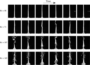
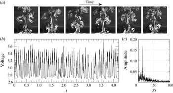
Evolution of a plume from laminar to pulsating state with increase in
 $Re$
for the case
 $Fr=0.1$
and
 $S=0.276$
(
 $Ri=72$
). Time difference between successive frames is 0.060 s. Field of view (FOV) of each image is 257 mm (width)
 $\times$
266 mm (height).

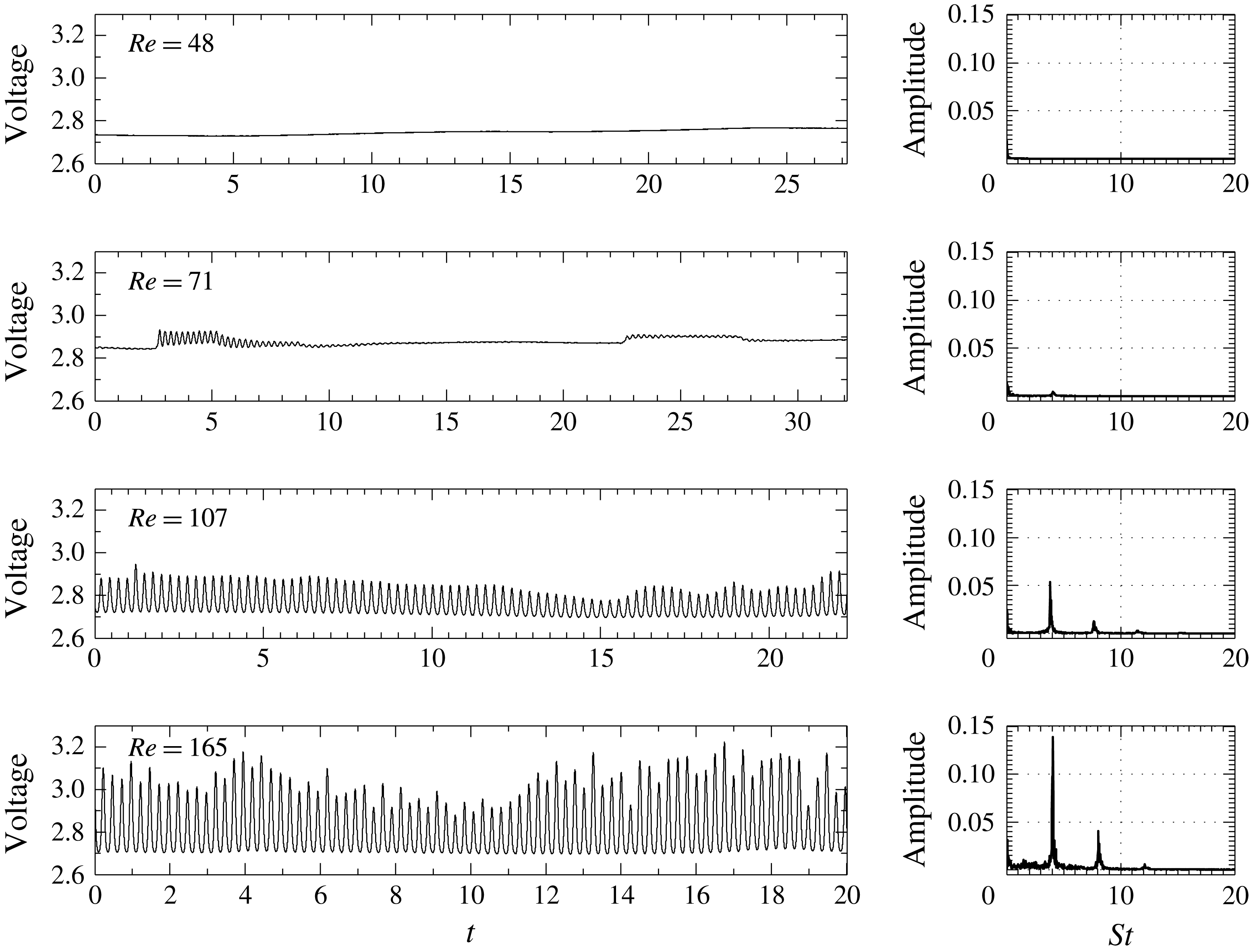
Hot-wire signal, and corresponding FFTs for the cases shown in figure 13.

Figure 13 shows the evolution of a plume with increase in
 $Re$
for the case
 $Fr=0.1$
and
 $S=0.276$
(
 $Ri=72$
). At each
 $Re$
, the temporal evolution of the plume is also shown to illustrate the periodic nature of vortex shedding once the plumes start oscillating. The corresponding voltage signals from hot-wire, and their fast Fourier transforms (FFT), calculated from the perturbation voltage (obtained by subtracting the time-averaged voltage), are presented in figure 14. For this case, the critical
 $Re$
obtained from instability analysis is
 ${\approx}$
90, as seen from figure 8.
At
 $Re=48$
, the plume assumes a long columnar shape. The corresponding hot-wire signal does not show any undulations and therefore, the state of the plume is steady laminar. With an increase in
 $Re$
to 71, the plume still maintains a long columnar shape with intermittent helical meandering and breakdown of the plume column in the far field as observed at
 $Re=71$
in figure 13. The corresponding hot-wire signal at
 $Re=71$
shows intermittent oscillations in the near field which decay over a period of time and the plume column returns to the steady state. These intermittent oscillations arise as the plumes approach critical conditions, close to the stability boundary (Maxworthy Reference Maxworthy1999). However, since the plume
 $Re$
(i.e. 71) is below critical
 $Re$
(i.e.
 ${\approx}90$
), these intermittent oscillations get damped by viscous diffusion over a period of time and the plumes remain stable. Further, these intermittent oscillations near the plume inlet lead to helical instabilities downstream, since low-density plumes are convectively unstable to helical perturbation modes (
 $m=1$
) in the self-similar plume regime (Chakravarthy et al.
Reference Chakravarthy, Lesshafft and Huerre2015).
With further increase in
 $Re$
beyond the critical
 $Re$
, the plume locks into an oscillatory state with periodic shedding of axisymmetric vortices in the vicinity of the nozzle lip as shown in figure 13 at
 $Re=107$
and 165. The hot-wire signal shows periodic oscillations with a characteristic frequency as seen from their FFTs (refer to
 $Re=107$
and 165 in figure 14). This oscillating instability observed in buoyant plumes is commonly termed as ‘puffing’ (Cetegen & Kasper Reference Cetegen and Kasper1996), and its dominant frequency is referred to as ‘puffing frequency’. Their FFTs also show lower amplitude peaks which correspond to the harmonics of the puffing frequency. The amplitude of the oscillations increases with an increase in
 $Re$
as observed in figure 14. This implies that at a fixed
 $Fr$
and
 $S$
, the intensity of oscillations increases with increase in
 $Re$
consistent with the growth rate variation observed in figure 6(b).
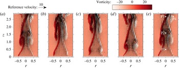
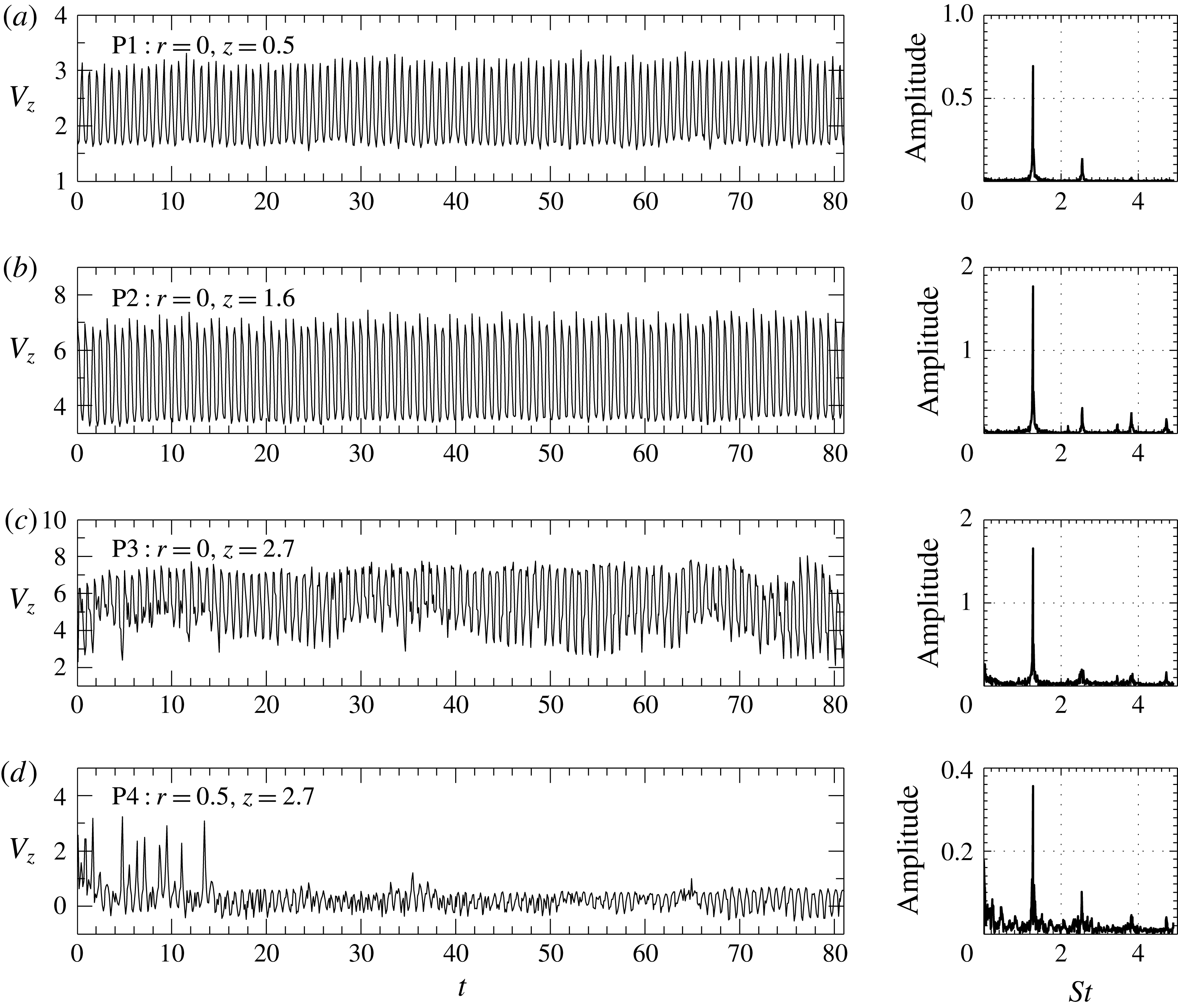
The instantaneous velocity fields obtained from PIV are used to investigate the spatial variation of puffing frequency in the near field. Figure 15 shows the instantaneous velocity fields overlapped onto their corresponding vorticity fields during a single puffing cycle. The velocity and vorticity fields clearly show the formation, growth and downstream convection of a puffing vortex as the plume undergoes this oscillatory instability. The axisymmetric puffing vortex in the near field elongates in the axial direction as it moves away from the inlet as seen in 15(a,e) and subsequently breaks down as observed from 15(b,c), thus leading to a more complex flow away from the source. To investigate the spatial variation of puffing frequency, the time traces of axial velocity at four different positions, P1, P2 and P3 along the centreline and P4 at plume periphery (refer to figure 15 e), are extracted and FFT analysis has been performed on these traces. The axial velocity variation with time at these four positions and their corresponding FFTs are presented in figure 16. The velocity traces show that the puffing is highly regular and periodic in the vicinity of the plume inlet. The FFTs obtained show a unique dominant frequency at all positions, which is a characteristic of a global instability.
Instantaneous velocity and vorticity fields obtained from PIV measurements at 50 Hz for the case
 $Re=329$
,
 $Fr=0.4$
and
 $S=0.276$
during 5 different instants of a typical puffing cycle. Puffing cycle starts at (a) and ends at (e), such that (a)
 ${\approx}$
(e). Time difference between successive velocity fields is 0.040 s. Puffing frequency for this case is
 $f=6.4$
Hz.

Axial velocity traces with time extracted at positions (a) P1, (b) P2, (c) P3 and (d) P4 marked in figure 15(e), and their corresponding FFTs.

4.3.2 Validation of stability boundaries
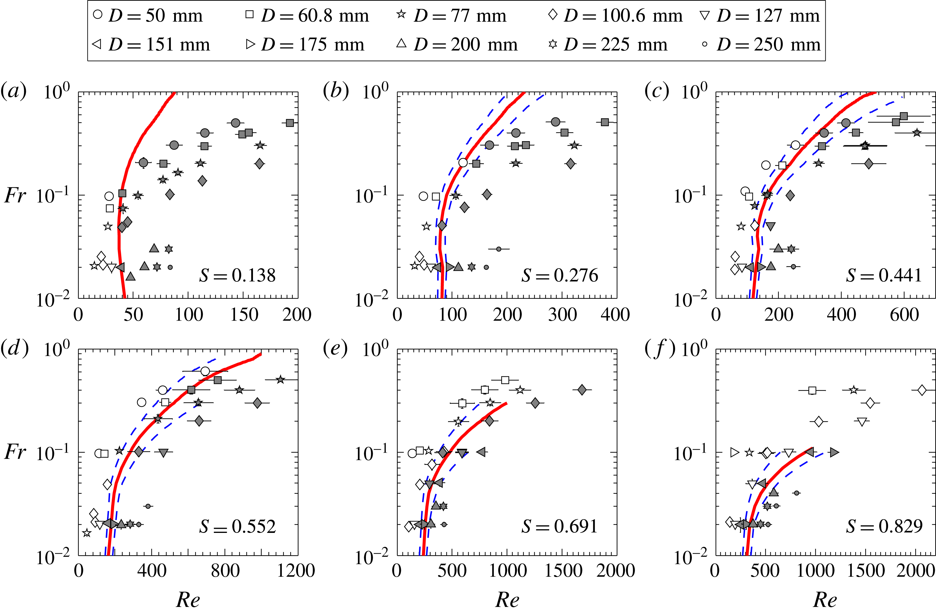
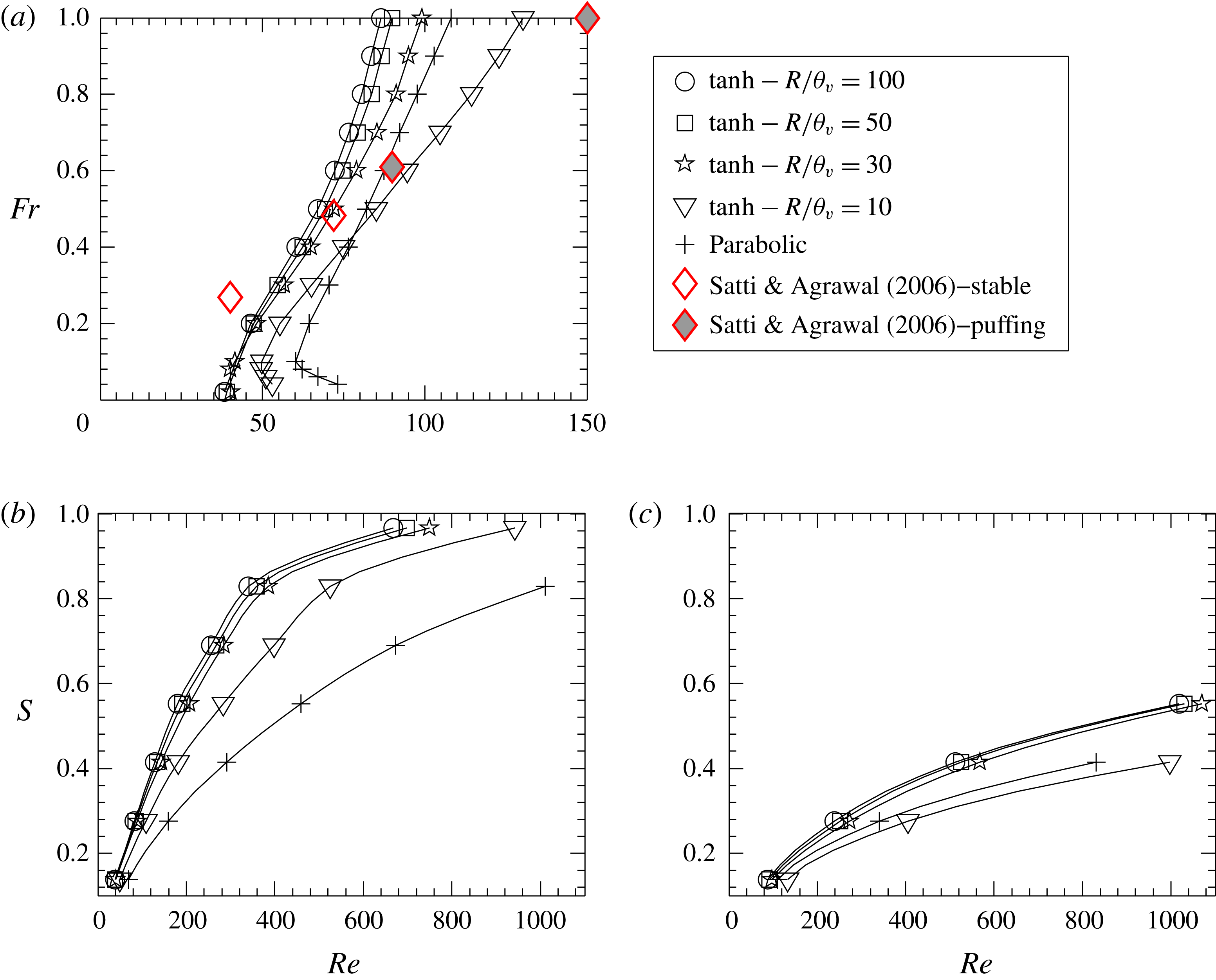
The state of the plume thus obtained using smoke-flow visualizations and hot-wire signal are mapped on the
 $Re{-}Fr$
plane and plotted in figure 17(a–f) for various density ratios along with the neutral curves obtained from global stability analysis. The transition map for helium plumes (
 $S=0.138$
) proves that the neutral stability curve effectively demarcated the regions of stable and puffing plumes (refer to figure 17
a). For plumes of helium–air mixtures i.e.
 $S>0.138$
, the transition region predicted by the instability analysis marginally deviates from the experiments, particularly at lower
 $Fr$
(refer to 17
b–f) The reason for this deviation at lower
 $Fr$
for plumes of helium–air mixtures can be attributed to the uncertainties in the density ratio
 $S$
, that arise from the errors in setting helium and air mass flow rates which have to be mixed to achieve a desired plume inlet density. For pure helium plumes, the uncertainty in density ratio is zero since no mixing takes place. For helium–air plumes, the maximum uncertainty in
 $S$
is evaluated as
 ${\approx}\pm 8\,\%$
. At each
 $S$
, the neutral curves corresponding to this maximum uncertainty are also presented as dashed lines in figure 17. After accounting for these uncertainties, it can be observed that the instability analysis effectively predicted the boundary separating the stable laminar plumes and the unstable puffing plumes.
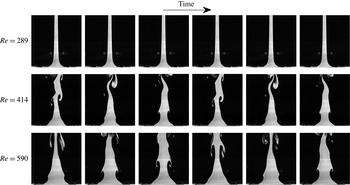
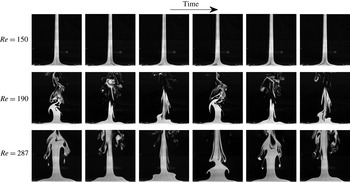
More importantly, contrary to the previous experiments of Cetegen (Reference Cetegen1997), puffing is also observed at density ratios
 $S>0.6$
in the present experiments as seen from 17(e–f), consistent with the predictions of the global stability analysis. Figures 18 and 19 show the evolution of plumes from laminar to puffing states for
 $S>0.6$
. These flow visualization images are shown with increasing
 $Re$
for the cases
 $Fr=0.1$
,
 $S=0.691$
(figure 18) and
 $Fr=0.02$
,
 $S=0.829$
(figure 19). Thus, these experiments confirm that puffing can occur in plumes even at higher density ratios. However, at higher
 $S$
, puffing is confined to plumes of lower
 $Fr$
and higher
 $Re$
, when compared to low
 $S$
plumes, which is consistent with the observation from instability analysis.
A plausible reason for the absence of puffing for
 $S>0.6$
in the experiments of Cetegen (Reference Cetegen1997) is that at higher
 $S$
, their plume investigations would have been confined to the globally stable region, i.e. either high
 $Fr$
or, low
 $Fr$
and low
 $Re$
. Unfortunately, we could not verify this claim since
 $Fr$
at which Cetegen (Reference Cetegen1997) performed experiments is not readily available in their paper.
Mapping of plume state on
 $Re{-}Fr$
plane for various
 $S$
, using ‘orifices’ of different diameters and comparison with neutral curves obtained from linear stability analysis. Open symbols correspond to the non-puffing plumes while filled symbols correspond to puffing plumes. The dashed lines are the neutral curves at maximum density uncertainty i.e. at
 $S\pm 8\,\%$
.

Evolution of a plume from laminar to pulsating state with increase in
 $Re$
for the case
 $Fr=0.1$
and
 $S=0.691$
(
 $Ri=31$
). Time difference between successive frames is 0.1 s. FOV of each image is the same as in figure 13.

Evolution of a plume from laminar to pulsating state with increase in
 $Re$
for the case
 $Fr=0.02$
and
 $S=0.829$
(
 $Ri=430$
). Time difference between successive frames is 0.2 s. FOV of each image is the same as in figure 13.

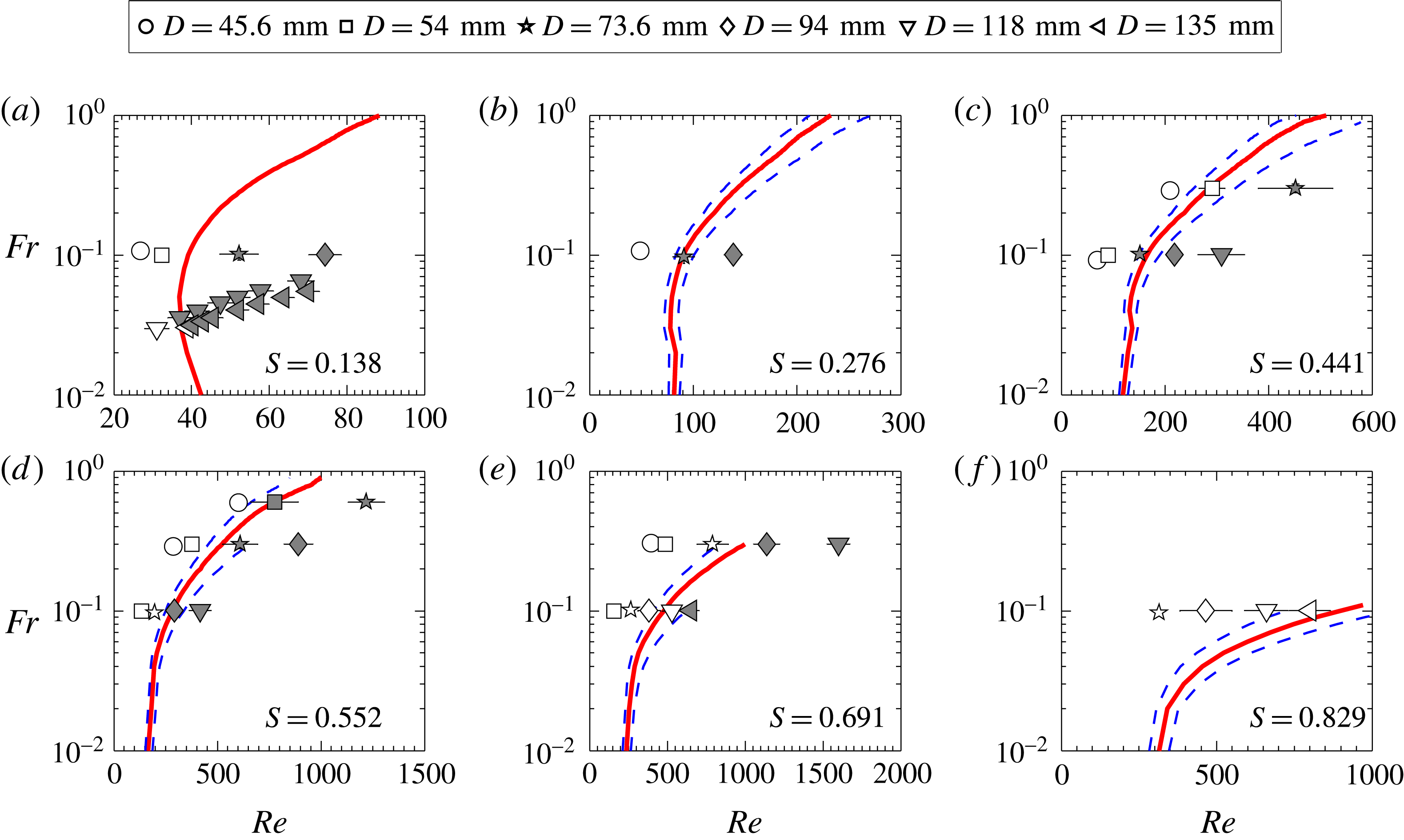
Transition maps similar to figure 17 obtained for ‘pipe nozzles’ of different diameters. The dashed lines are the neutral curves at maximum density uncertainty i.e. at
 $S\pm 6\,\%$
.

Similar experiments are carried out for plumes emanating from pipe nozzles, and the plume states obtained from these experiments are mapped on the
 $Re{-}Fr$
plane in figure 20. These experiments also confirm the presence of puffing at higher density ratios, for example at
 $S=0.691$
in figure 20. A comparison with stability boundaries obtained from linear stability analysis shows that a change in the plume inlet conditions does not have an impact in the plume transition from laminar to puffing state. This issue will be further investigated later in § 4.4 where the effect of the change in inlet velocity profile on the global stability characteristics of plumes is investigated.
4.3.3 Puffing frequency
The earlier experiments and global instability analysis showed that the
 $St$
of puffing scales well with
 $Ri$
. Therefore, the puffing frequencies measured in the experiments are presented in terms of
 $St$
variation with
 $Ri$
and compared with the
 $St{-}Ri$
correlations obtained from instability analysis (refer to figure 12). Also,
 $St$
obtained in experiments of Cetegen & Kasper (Reference Cetegen and Kasper1996) are presented to highlight the discrepancy observed between their experiments and global instability analysis regarding the
 $Ri$
at which the plume frequencies switch from primary to secondary mode.
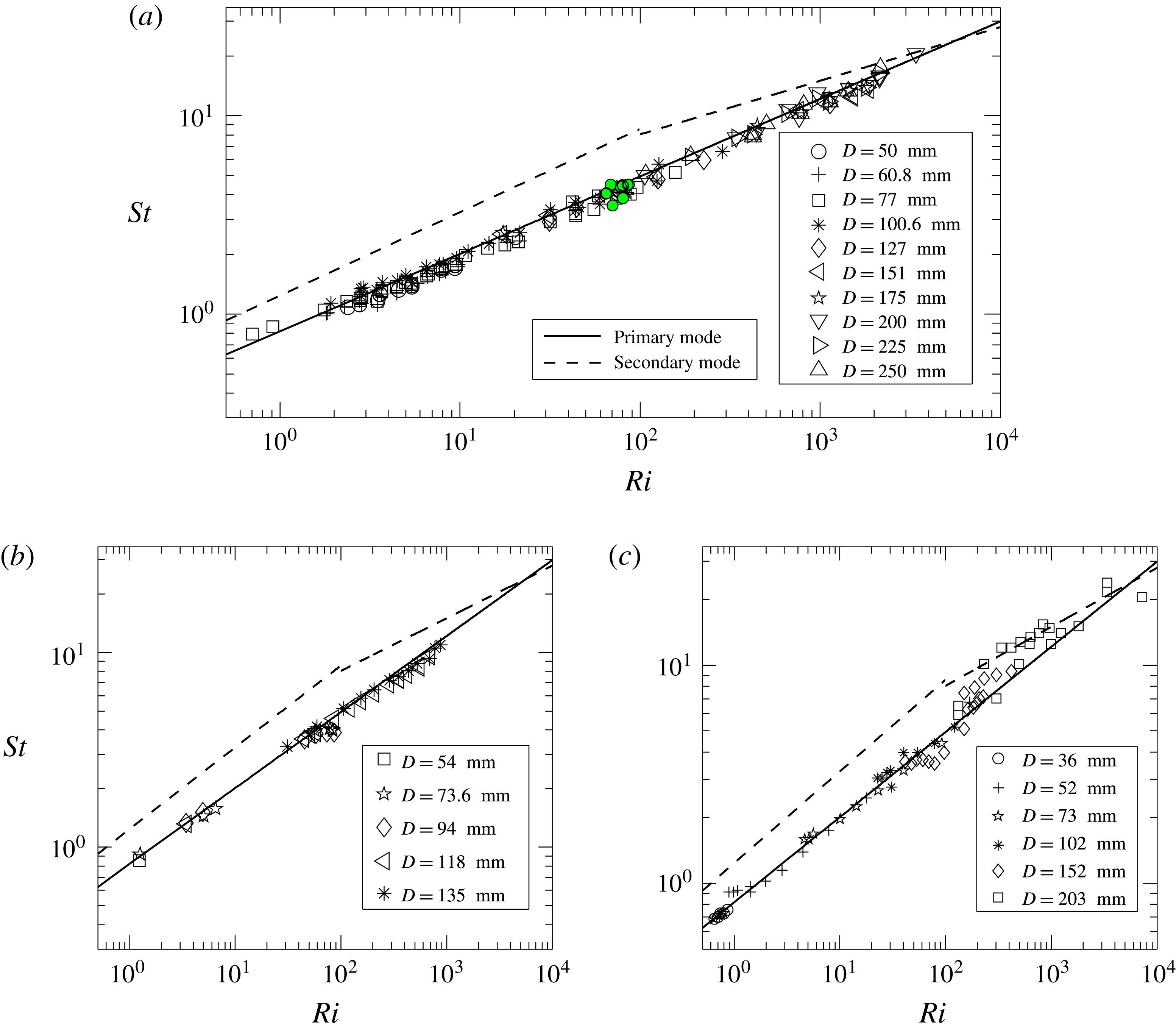
Strouhal number variation with Richardson number for the plumes emanating from (a) orifices and (b) pipe nozzles in the present experiments. (c) Strouhal number variation with Richardson number extracted from figure 5 of Cetegen & Kasper (Reference Cetegen and Kasper1996) for plumes emanating from their pipe nozzles. The solid and dashed lines correspond to
 $St{-}Ri$
correlations obtained for primary and secondary modes in figure 12 using global linear stability analysis.

The
 $St$
variation with
 $Ri$
obtained in the present experiments using various orifices is plotted in figure 21(a) and compared with the correlations obtained from stability analysis. The puffing frequencies closely follow the power-law variation corresponding to the primary mode in the entire
 $Ri$
range investigated for orifices. This is consistent with stability analysis where the primary mode exhibited dominant frequency for
 $Ri<6000$
. Similar observations are made in case of plumes emanating from pipe nozzles whose
 $St$
variation with
 $Ri$
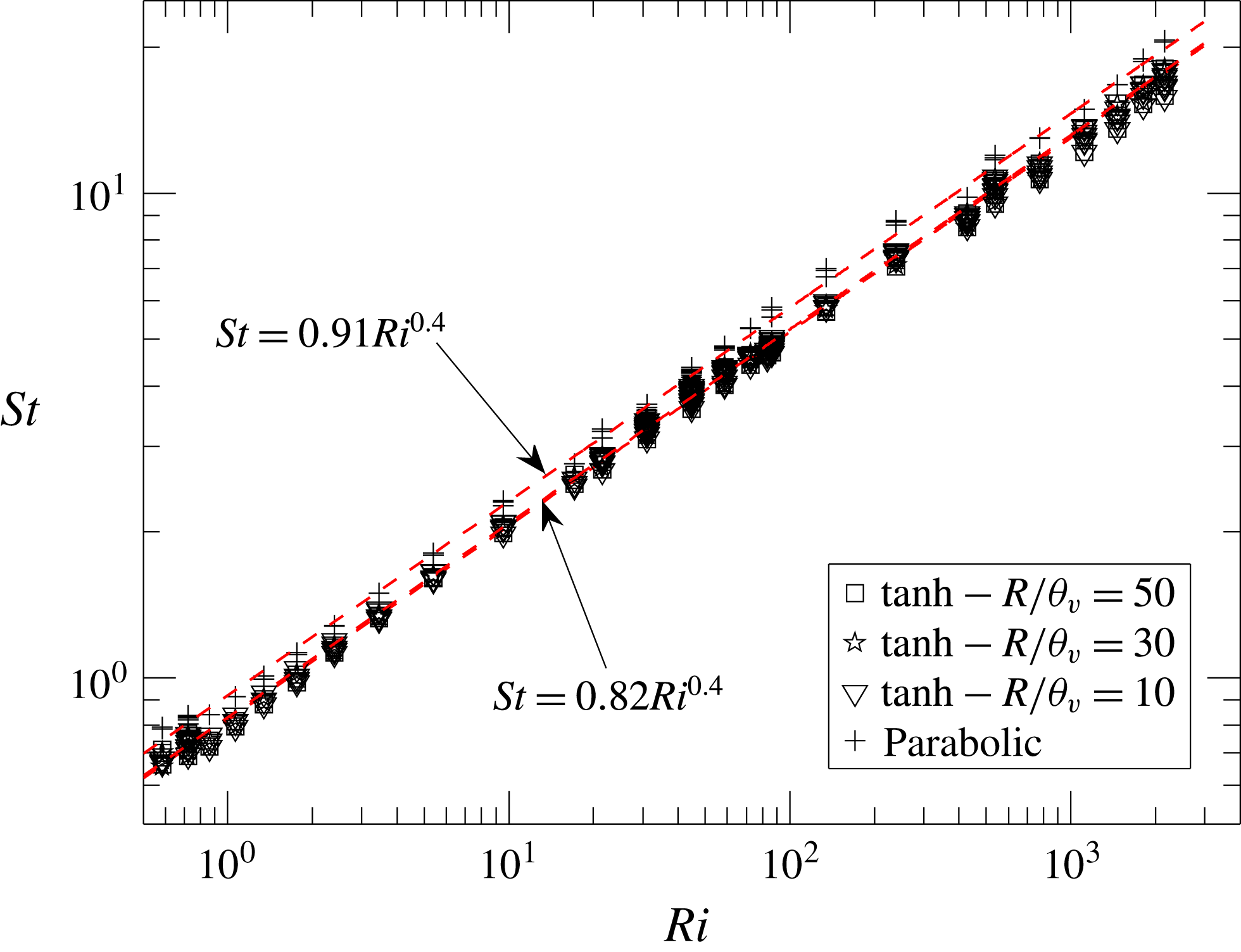
is plotted in figure 21(b). A least square power-law fit to the
 $St{-}Ri$
variation yields the correlations
 $St=0.78Ri^{0.39}$
and
 $St=0.82Ri^{0.38}$
for orifice and pipe-nozzle inlet configurations respectively, which are in good agreement with the puffing frequency correlation of primary global mode, i.e.
 $St=0.82Ri^{0.39}$
, and with the correlation
 $St=0.8Ri^{0.38}$
obtained by Cetegen & Kasper (Reference Cetegen and Kasper1996). Also, a comparison of
 $St{-}Ri$
correlations obtained in experiments using orifices and pipe nozzles shows that a change in plume inlet configuration leads to a negligible variation in puffing frequencies.
Turbulent nature of plumes at high
 $Ri$
. (a) Snapshots at various phases in a puffing cycle for a plume of
 $Ri=962$
(
 $Re=69$
,
 $Fr=0.03$
and
 $S=0.138$
), (b) its hot-wire signal and (c) FFT.

However, the present data differ from the experiments of Cetegen & Kasper (Reference Cetegen and Kasper1996) in terms of
 $Ri$
at which the transition of plume frequencies from primary to secondary mode occurs. As noted earlier, Cetegen & Kasper (Reference Cetegen and Kasper1996) obtained puffing frequencies by measuring velocity fluctuations along the centreline, for plumes emanating from pipe nozzles of
 $L/D$
in range of 3–10. Figure 21(c) shows their
 $St{-}Ri$
data, extracted from figure 5 of Cetegen & Kasper (Reference Cetegen and Kasper1996) and compared with the present stability analysis. The puffing
 $St$
in their experiments closely follow the primary mode till
 $Ri=100$
. Thereafter, for
 $Ri>100$
, their
 $St$
switches to the secondary mode with a fewer modes following the primary mode, as seen in figure 21(c). However, this switch in frequency scaling is not observed in the present experiments for both orifice and pipe-nozzle configurations, and is also in disagreement with global stability analysis, which predicted the primary mode to attain higher growth rate till
 $Ri=6000$
and the switch in frequency scaling for
 $Ri>6000$
. Cetegen & Kasper (Reference Cetegen and Kasper1996) attributed this switch in frequency scaling to the turbulent nature of puffing vortex and vigorous mixing in the plume near field observed beyond
 $Ri$
range 100–500 in their experiments. To examine this argument and compare with the present work, we looked into the flow field of a plume with
 $Ri>500$
obtained in the present experiments.
Figure 22(a) shows a typical helium plume of
 $Ri=962$
at different phases of puffing. The hot-wire signal and corresponding FFT for this case are plotted in 22(b) and 22(c) respectively. It is evident that the near field of the plume is highly turbulent when compared to the plumes at lower
 $Ri$
(for example, see figures 13 and 18), consistent with the argument of Cetegen & Kasper (Reference Cetegen and Kasper1996). However, in the present experiments, though the puffing in these high
 $Ri$
plumes is relatively turbulent, their puffing frequencies closely followed the frequency correlation of primary mode without any switch, as predicted by linear theory. Furthermore, it is interesting to note that although the plumes turn turbulent at larger
 $Ri$
, their frequencies match closely with the predictions from the linear theory. This is also true for high
 $Re$
turbulent plumes (
 $Re\approx 3200$
,
 $Ri\approx 76$
) of O’hern et al. (Reference O’hern, Weckman, Gerhart, Tieszen and Schefer2005), whose puffing frequencies are shown using filled symbols in figure 21(a). This is because, even far from critical conditions, the large-scale dynamics of these plumes is governed by puffing, while the onset of secondary Rayleigh–Taylor instabilities contribute substantially to their turbulent nature (O’hern et al.
Reference O’hern, Weckman, Gerhart, Tieszen and Schefer2005). In turbulent plumes, the effect of these secondary instabilities on their puffing frequencies seems to be marginal.
Ascertaining the exact reason for this discrepancy between the earlier and present experiments is beyond the scope of this study. However, it is conjectured that in the experiments of Cetegen & Kasper (Reference Cetegen and Kasper1996), the disturbances at plume inlet might have played a role in the earlier switching of plumes from primary to secondary mode (i.e. at
 $Ri=100$
–500). As noted earlier in § 3, a major difference between the set-ups used in these two works is the usage of a separate mixing chamber with silencers and sound absorbing foam, to minimize the disturbances/forcing in the settling chamber that arise due to flow noise and pressure fluctuations. Without these, it is observed that the plume is prone to forcing and disturbances at the inlet.
As the experiments are performed with orifices and pipe nozzles, we further investigate the effect of a change in inlet velocity profiles on plume instability. Therefore, in the following section, we investigate the same using global stability analysis.
4.4 Effect of inlet velocity profile
As stated earlier, the stability analysis results presented till now are obtained for top-hat inlet profiles (B 1) and (B 2) by setting velocity and mass fraction steepness parameters (
 $R/\unicode[STIX]{x1D703}_{v}$
and
 $R/\unicode[STIX]{x1D703}_{y}$
) as 100. In this section, we investigated the effect of inlet velocity profile on transition and puffing frequencies of plumes. To accomplish this, the mass-fraction profile is kept unaltered (
 $R/\unicode[STIX]{x1D703}_{y}=100$
) and the base flows are calculated for different tanh velocity profiles by varying steepness parameter as
 $R/\unicode[STIX]{x1D703}_{v}=100$
, 50, 30 and 10, and for a parabolic inlet velocity profile. Subsequently, stability analysis is performed on these newly obtained base flows. Physically, in experiments, this study is equivalent to the effect of an increase in nozzle
 $L/D$
ratio on plume stability characteristics.
Figure 23(a) shows the neutral curves obtained for tanh velocity profiles with
 $R/\unicode[STIX]{x1D703}_{v}=100$
, 50, 30, 10 and for a parabolic velocity profile on the
 $Re{-}Fr$
plane at
 $S=0.138$
(pure He plumes). To investigate the effect of
 $S$
, neutral curves are obtained on
 $Re{-}S$
plane at
 $Fr=0.02$
and
 $Fr=1$
and are plotted in 23(b) and 23(c) respectively. In figure 23(a), the neutral curve obtained for parabolic velocity profile is compared with Satti & Agrawal (Reference Satti and Agrawal2006). For helium gas plumes with parabolic inlet velocity profile and constant inlet mass fraction, Satti & Agrawal (Reference Satti and Agrawal2006) carried out numerical simulations in
 $Re$
range 40–150 and
 $Fr$
range 0.27–1. They reported that these plumes changed from steady to oscillatory state at approximately
 $Re=90$
and
 $Fr=0.6$
, which is in good agreement with the stability boundary obtained from linear stability analysis for parabolic inlet velocity profiles.
Neutral curves obtained for various inlet velocity profiles (a) for a fixed
 $S=0.138$
on
 $Re{-}Fr$
plane and, for Froude numbers (b)
 $Fr=0.02$
and (c)
 $Fr=1$
on
 $Re{-}S$
plane.

Figure 23(a–c) shows that plumes with steeper inlet velocity profiles (higher
 $R/\unicode[STIX]{x1D703}_{v}$
, near top-hat) are more unstable. Puffing initiates in these plumes at low
 $Re$
, as their growth rates are higher when compared to smoother velocity profiles (near parabolic). The change in critical
 $Re$
with decrease in
 $R/\unicode[STIX]{x1D703}_{v}$
is marginal at higher
 $R/\unicode[STIX]{x1D703}_{v}$
. For example, the critical
 $Re$
increases by a maximum of about 6 % and 15 % by decreasing
 $R/\unicode[STIX]{x1D703}_{v}$
from 100 to 50 and 100 to 30 respectively. This maximum increase occurs at high
 $Fr$
, while at low
 $Fr$
, this increase is smaller. With a further decrease in steepness parameter, the increase in critical
 $Re$
is significant. The minimum and maximum increase in critical
 $Re$
are approximately 20 % and 95 % respectively for a decrease in
 $R/\unicode[STIX]{x1D703}_{v}$
from 100 to 10. Also, figure 23(b,c) shows that a parabolic velocity profile is more stable at lower
 $Fr$
, while smoother tanh profiles are more stable at higher
 $Fr$
. Thus, from the present analysis, we conclude that the shape of the inlet velocity profile impacts the plume transition only for nozzles with larger
 $L/D$
ratios, which gives smoother velocity profiles at plume inlet. For steeper velocity profiles, the impact is insignificant. The experiments in the present work are performed using orifices and smaller
 $L/D$
pipe nozzles (in range 3.3–7.2), with a flat mesh screen across their exit plane. In the present experiments, a change in the inlet configuration had an insignificant effect on plume transition as noted in the previous section since both these inlet configurations give steeper velocity profiles at plume inlet.
Effect of inlet velocity profiles on puffing frequency.

To consider the effect of inlet velocity profile variation on puffing frequencies,
 $St{-}Ri$
correlations obtained for various velocity profiles are plotted in figure 24. For tanh velocity profiles, the effect of steepness parameter on
 $St$
is negligible and the
 $St{-}Ri$
power-law correlation remains approximately the same for all
 $R/\unicode[STIX]{x1D703}_{v}$
. For parabolic velocity profile, the puffing frequencies are marginally higher than the top-hat velocity profiles. Overall, we conclude that the shape of the inlet velocity profile only affects the plume transition in case of smoother velocity profiles and its effect on puffing frequency is marginal. The relatively negligible effect of velocity profile variation on plume puffing frequencies is expected, since the
 $St$
is impacted only by buoyancy as seen in § 4.2.2.
Note that the neutral curves and global frequencies in figures 23 and 24 respectively, are presented only for the primary mode. This is due to the reason that, for any velocity profile, the primary mode always attained higher growth rate than the secondary mode in the entire
 $Ri$
range for which the effect of inlet velocity profile on plume instability has been investigated.
However, the top-hat velocity profile (B 1) does not truly represent the velocity profiles the arise at the outlet of finite length pipe nozzles. The smoothness parameter
 $R/\unicode[STIX]{x1D703}_{v}$
in velocity profile (B 1) gives a qualitative representation of the effect of smoothness of the velocity profile on plume instability. Therefore to ascertain the effect of realistic velocity profiles that arise at the exit of finite length pipe nozzles of increasing
 $L/D$
on base flow development and plume instability, we also carried out global stability computations for the base flows generated using these realistic inlet velocity profiles. The procedure adopted for this investigation, and the corresponding results, are presented in appendix C.
4.5 Instability mechanism: effects of baroclinic and gravitational torques
The above discussions regarding the plume behaviour from global linear stability analysis and experiments lead us to investigate the possible mechanisms responsible for puffing in plumes. Of all the parameters investigated, it is clear that the most important parameters that govern plume transition and puffing frequencies are
 $Fr$
and
 $S$
i.e. the global instability in plumes is largely impacted by the gravity and density difference via buoyancy. The reason for such dependence can probably be understood if we explore the mechanism(s) by which the flow perturbations interact with the base flow and destabilize the steady laminar plumes. Since the global instability manifests as vortical structures, we follow an approach based on vortex dynamics. To understand the mechanism of perturbation vorticity (
 $\unicode[STIX]{x1D73B}^{\prime }=\unicode[STIX]{x1D735}\times \boldsymbol{v}^{\prime }$
) generation, an equation for perturbation vorticity has been derived. Dividing the linearized perturbation momentum equation (2.10) by the mean density
 $\overline{\unicode[STIX]{x1D70C}}$
and eliminating
 $\overline{\boldsymbol{V}}\boldsymbol{\cdot }\unicode[STIX]{x1D735}\overline{\boldsymbol{V}}$
using the base flow momentum equation
 $$\begin{eqnarray}\displaystyle \displaystyle \overline{\boldsymbol{V}}\boldsymbol{\cdot }\unicode[STIX]{x1D735}\overline{\boldsymbol{V}} & = & \displaystyle -{\displaystyle \frac{\unicode[STIX]{x1D735}\overline{p}}{\overline{\unicode[STIX]{x1D70C}}}}+\left(1-{\displaystyle \frac{1}{\overline{\unicode[STIX]{x1D70C}}}}\right){\displaystyle \frac{\boldsymbol{g}}{Fr^{2}}}+\text{viscous terms},\end{eqnarray}$$
we rewrite (2.10) in its modified form
 $$\begin{eqnarray}\displaystyle \displaystyle {\displaystyle \frac{\unicode[STIX]{x2202}\boldsymbol{v}^{\prime }}{\unicode[STIX]{x2202}t}}+\overline{\boldsymbol{V}}\boldsymbol{\cdot }\unicode[STIX]{x1D735}\boldsymbol{v}^{\prime }+\boldsymbol{v}^{\prime }\boldsymbol{\cdot }\unicode[STIX]{x1D735}\overline{\boldsymbol{V}} & = & \displaystyle \left[-{\displaystyle \frac{\unicode[STIX]{x1D735}p^{\prime }}{\overline{\unicode[STIX]{x1D70C}}}}+{\displaystyle \frac{\unicode[STIX]{x1D70C}^{\prime }}{\overline{\unicode[STIX]{x1D70C}}^{2}}}\unicode[STIX]{x1D735}\overline{p}\right]+{\displaystyle \frac{\unicode[STIX]{x1D70C}^{\prime }}{\overline{\unicode[STIX]{x1D70C}}^{2}}}{\displaystyle \frac{\boldsymbol{g}}{Fr^{2}}}+\text{viscous terms}.\end{eqnarray}$$
Assuming the laminar plume to be long and thin (as observed in flow visualizations of laminar plumes in figures 13, 18 and 19), the boundary layer approximation can be invoked where, pressure gradients become negligible in radial and axial directions (
 $\unicode[STIX]{x1D735}\overline{p}=0$
) as the ambient pressure variation is hydrostatic. The perturbation vorticity equation is now obtained by taking the curl of modified linearized perturbation momentum equation (4.2) as
 $$\begin{eqnarray}\displaystyle & & \displaystyle {\displaystyle \frac{\unicode[STIX]{x2202}\unicode[STIX]{x1D73B}^{\prime }}{\unicode[STIX]{x2202}t}}+(\overline{\boldsymbol{V}}\boldsymbol{\cdot }\unicode[STIX]{x1D735})\unicode[STIX]{x1D73B}^{\prime }+(\boldsymbol{v}^{\prime }\boldsymbol{\cdot }\unicode[STIX]{x1D735})\overline{\unicode[STIX]{x1D734}}=-\unicode[STIX]{x1D73B}^{\prime }(\unicode[STIX]{x1D735}\boldsymbol{\cdot }\overline{\boldsymbol{V}})-\overline{\unicode[STIX]{x1D734}}(\unicode[STIX]{x1D735}\boldsymbol{\cdot }\boldsymbol{v}^{\prime })+(\unicode[STIX]{x1D73B}^{\prime }\boldsymbol{\cdot }\unicode[STIX]{x1D735})\overline{\boldsymbol{V}}+(\overline{\unicode[STIX]{x1D734}}\boldsymbol{\cdot }\unicode[STIX]{x1D735})\boldsymbol{v}^{\prime }\nonumber\\ \displaystyle & & \displaystyle \qquad +\,{\displaystyle \frac{\unicode[STIX]{x1D735}\overline{\unicode[STIX]{x1D70C}}\times \unicode[STIX]{x1D735}p^{\prime }}{\overline{\unicode[STIX]{x1D70C}}^{2}}}+\unicode[STIX]{x1D735}\left({\displaystyle \frac{\unicode[STIX]{x1D70C}^{\prime }}{\overline{\unicode[STIX]{x1D70C}}^{2}}}\right)\times {\displaystyle \frac{\boldsymbol{g}}{Fr^{2}}}+\text{viscous terms},\end{eqnarray}$$
where,
 $\overline{\unicode[STIX]{x1D734}}=\overline{\unicode[STIX]{x1D735}}\times \overline{\boldsymbol{V}}$
is the base flow vorticity. In the above equation, the terms on the left-hand side represent the rate of change of vorticity of a fluid element because of perturbations. On the right-hand side, the first two terms represent the contribution of perturbations to the reduction (enhancement) in vorticity arising from the fluid expansion (compression) (Green Reference Green2012). The third and fourth terms on the right-hand side represent the vorticity intensification due to vortex stretching by the flow perturbations. The fifth term on the right-hand side represents the perturbation baroclinic torque which arises due to the misalignment of mean density and pressure perturbation gradients. The sixth term on the right-hand side represents the perturbation gravitational torque which arises due to the misalignment of density perturbation and mean flow density gradients with gravity. In variable-density shear layers, these two torques act as sources of vorticity perturbations and contribute to the destabilization of mean vorticity generated by the steady base flow. Note that the contribution of viscous diffusive terms is not considered here, since at these moderate
 $Re$
, the viscous terms usually stabilize the flow field by smoothening out the vorticity perturbations (Nichols et al.
Reference Nichols, Schmid and Riley2007). The observation from figures 6(b) and 7(b) that
 $\unicode[STIX]{x1D714}_{i}$
decreases with a decrease in
 $Re$
also shows the stabilizing effect of viscosity.
The effects of perturbation baroclinic and gravitational torques on the plume stability are quantitatively assessed by solving the eigenvalue problem with modified dispersion relations, in which each of these two torques is eliminated by counterbalancing it with appropriate forcing. The procedure implemented for this, as described below, follows the idea of Lesshafft & Huerre (Reference Lesshafft and Huerre2007) who investigated the role of baroclinicity in instability of hot jets.
In the presence of a source term
 $\boldsymbol{{\mathcal{S}}}=({\mathcal{S}}_{r}\boldsymbol{e}_{\boldsymbol{r}},{\mathcal{S}}_{\unicode[STIX]{x1D703}}\boldsymbol{e}_{\unicode[STIX]{x1D73D}},{\mathcal{S}}_{z}\boldsymbol{e}_{\boldsymbol{z}})$
, the linearized disturbance momentum equation (2.10) becomes
 $$\begin{eqnarray}\overline{\unicode[STIX]{x1D70C}}{\displaystyle \frac{\unicode[STIX]{x2202}\boldsymbol{v}^{\prime }}{\unicode[STIX]{x2202}t}}+\overline{\unicode[STIX]{x1D70C}}\left(\overline{\boldsymbol{V}}\boldsymbol{\cdot }\unicode[STIX]{x1D735}\boldsymbol{v}^{\prime }+\boldsymbol{v}^{\prime }\boldsymbol{\cdot }\unicode[STIX]{x1D735}\overline{\boldsymbol{V}}\right)+\unicode[STIX]{x1D70C}^{\prime }\overline{\boldsymbol{V}}\boldsymbol{\cdot }\unicode[STIX]{x1D735}\overline{\boldsymbol{V}}=-\unicode[STIX]{x1D735}p^{\prime }+\unicode[STIX]{x1D70C}^{\prime }{\displaystyle \frac{\boldsymbol{g}}{Fr^{2}}}+\text{viscous terms}+\boldsymbol{{\mathcal{S}}}\end{eqnarray}$$
and the vorticity perturbation
 $\unicode[STIX]{x1D73B}^{\prime }$
evolves with the additional source term as
 $$\begin{eqnarray}\displaystyle & & \displaystyle {\displaystyle \frac{\unicode[STIX]{x2202}\unicode[STIX]{x1D73B}^{\prime }}{\unicode[STIX]{x2202}t}}+(\overline{\boldsymbol{V}}\boldsymbol{\cdot }\unicode[STIX]{x1D735})\unicode[STIX]{x1D73B}^{\prime }+(\boldsymbol{v}^{\prime }\boldsymbol{\cdot }\unicode[STIX]{x1D735})\overline{\unicode[STIX]{x1D734}}=-\unicode[STIX]{x1D73B}^{\prime }(\unicode[STIX]{x1D735}\boldsymbol{\cdot }\overline{\boldsymbol{V}})-\overline{\unicode[STIX]{x1D734}}(\unicode[STIX]{x1D735}\boldsymbol{\cdot }\boldsymbol{v}^{\prime })+(\unicode[STIX]{x1D73B}^{\prime }\boldsymbol{\cdot }\unicode[STIX]{x1D735})\overline{\boldsymbol{V}}+(\overline{\unicode[STIX]{x1D734}}\boldsymbol{\cdot }\unicode[STIX]{x1D735})\boldsymbol{v}^{\prime }\nonumber\\ \displaystyle & & \displaystyle \qquad +\,{\displaystyle \frac{\unicode[STIX]{x1D735}\overline{\unicode[STIX]{x1D70C}}\times \unicode[STIX]{x1D735}p^{\prime }}{\overline{\unicode[STIX]{x1D70C}}^{2}}}+\unicode[STIX]{x1D735}\left({\displaystyle \frac{\unicode[STIX]{x1D70C}^{\prime }}{\overline{\unicode[STIX]{x1D70C}}^{2}}}\right)\times {\displaystyle \frac{\boldsymbol{g}}{Fr^{2}}}+\text{viscous terms}+\unicode[STIX]{x1D735}\times \left({\displaystyle \frac{\boldsymbol{{\mathcal{S}}}}{\overline{\unicode[STIX]{x1D70C}}}}\right).\end{eqnarray}$$
In (4.5), the last term is the torque generated because of forcing
 $\boldsymbol{{\mathcal{S}}}$
. Following Lesshafft & Huerre (Reference Lesshafft and Huerre2007), in order to eliminate the effect of perturbation baroclinic or gravitational torques, the source terms are selected so as to satisfy the constraints
 $$\begin{eqnarray}\unicode[STIX]{x1D735}\times \left({\displaystyle \frac{\boldsymbol{{\mathcal{S}}}}{\overline{\unicode[STIX]{x1D70C}}}}\right)=-{\displaystyle \frac{\unicode[STIX]{x1D735}\overline{\unicode[STIX]{x1D70C}}\times \unicode[STIX]{x1D735}p^{\prime }}{\overline{\unicode[STIX]{x1D70C}}^{2}}}\quad \text{or}\quad \unicode[STIX]{x1D735}\times \left({\displaystyle \frac{\boldsymbol{{\mathcal{S}}}}{\overline{\unicode[STIX]{x1D70C}}}}\right)=-\unicode[STIX]{x1D735}\left({\displaystyle \frac{\unicode[STIX]{x1D70C}^{\prime }}{\overline{\unicode[STIX]{x1D70C}}^{2}}}\right)\times {\displaystyle \frac{\boldsymbol{g}}{Fr^{2}}}\end{eqnarray}$$
respectively, which result in the respective forcing terms in (4.5) as
 $$\begin{eqnarray}\boldsymbol{{\mathcal{S}}}=p^{\prime }{\displaystyle \frac{\unicode[STIX]{x1D735}\overline{\unicode[STIX]{x1D70C}}}{\overline{\unicode[STIX]{x1D70C}}}}\quad \text{or}\quad \boldsymbol{{\mathcal{S}}}={\displaystyle \frac{1}{Fr^{2}}}{\displaystyle \frac{\unicode[STIX]{x1D70C}^{\prime }}{\overline{\unicode[STIX]{x1D70C}}}}\boldsymbol{e}_{\boldsymbol{z}}.\end{eqnarray}$$
Thus, the effects of baroclinic and gravitational torques are investigated independently by counterbalancing each torque using the obtained forcing terms. A modified dispersion relation is formulated using the modified momentum perturbation equation (4.4), along with the continuity (2.9) and mass fraction (2.11) equations, and solved as an eigenvalue problem. Since plumes exhibit global instability only for axisymmetric perturbations, the present analysis is confined to axisymmetric perturbations, however, the equations (4.5) and (4.7) are valid for complete three-dimensional perturbations.
The analysis has been performed in the
 $Fr$
range 0.03–3 for various
 $Re$
and
 $S$
. The growth rates of the primary mode, thus obtained by eliminating baroclinic or gravitational torques for various cases, are normalized by their corresponding actual growth rates (obtained using full equation without eliminating any terms,
 $\unicode[STIX]{x1D714}_{i,fulleq}$
) and presented in figure 25. For all four cases considered for this study (i.e.
 $Re=$
600, 800 and 1000 at
 $S=$
0.276, and
 $Re=1000$
at
 $S=0.414$
, refer to figure 25), plumes are unstable in the entire
 $Fr$
range with positive
 $\unicode[STIX]{x1D714}_{i,fulleq}$
, as seen from the neutral stability curves in figure 8. If elimination of one of these two torques results in
 $\unicode[STIX]{x1D714}_{i}/\unicode[STIX]{x1D714}_{i,fulleq}<0$
, then it is considered that the elimination of the corresponding torque has a stabilizing effect on plume. Otherwise, its effect is considered to be destabilizing when
 $\unicode[STIX]{x1D714}_{i}/\unicode[STIX]{x1D714}_{i,fulleq}>0$
.
Normalized growth rates of primary mode obtained by elimination of perturbation baroclinic torque (grey filled) and gravitational torque (black filled) from governing equations.

With the elimination of perturbation baroclinic torque from the governing equations, the plumes remain unstable at lower
 $Fr$
(for instance around 0.03) where the growth rates of the primary mode remain closer to
 $\unicode[STIX]{x1D714}_{i,fulleq}$
(see figure 25). However, with an increase in
 $Fr$
from 0.03 to 3, these growth rates start reducing and eventually, the modes shift to the stable half-plane and the plumes become stable. These growth rates tend to decay rapidly with a further increase in
 $Fr$
, thus further stabilizing these plumes as observed in figure 25. Therefore, by removing baroclinic torque, high
 $Fr$
plumes stabilize, while low
 $Fr$
plumes remain unstable. At low
 $Fr$
, the gravitational effects dominate over the inertial effects and therefore, buoyancy becomes the primary destabilizing force.
Elimination of the perturbation gravitational torque from the governing equations has an exactly opposite effect on plume instability. By eliminating the gravitational torque, the plumes stabilize at lower
 $Fr$
as they attain negative growth rates (refer figure 25). With an increase in
 $Fr$
, the growth rates start increasing and the plumes become unstable. At higher
 $Fr$
, these plumes tend to attain the growth rates closer to
 $\unicode[STIX]{x1D714}_{i,fulleq}$
. Therefore, elimination of perturbation gravitational torque stabilize the plumes at lower
 $Fr$
, and plumes of higher
 $Fr$
remain unstable where the buoyancy effects are negligible.
Based on the above observations, it may therefore be concluded that, at lower
 $Fr$
(i.e.
 $Fr\ll 0.5$
), the perturbation gravitational torque becomes the dominant destabilizing mechanism and the effect of perturbation baroclinic torque on plume instability becomes marginal. Conversely, at higher
 $Fr$
(i.e.
 $Fr\gg 0.5$
), the perturbation baroclinic torque becomes the dominant destabilizing mechanism and the perturbation gravitational torque effects become marginal. The growth rates obtained by eliminating each of these two torques are found to cross over each other (marked as
 $\times$
in figure 25) in
 $Fr$
range 0.45–0.5. Therefore, for intermediate
 $Fr$
i.e. around 0.5 which correspond to the majority of the cases investigated in the present study, the baroclinic and gravitational torques generated by the perturbations become equally important and both these mechanisms contribute to the destabilization of plumes. By eliminating both these torques together from the governing equations, it is observed that the discrete primary mode vanishes and the flow remains stable for all the inlet parameters considered here.
Using the identified mechanisms, we attempt to qualitatively explain the differences in oscillation frequency dependencies observed for different
 $Fr$
ranges. In buoyant jets of
 $2\leqslant Fr\leqslant \infty$
, Nichols et al. (Reference Nichols, Schmid and Riley2007) observed that the frequencies of global instability are largely impacted by
 $S$
, which signifies the density difference between the source and ambient, while they are least impacted by
 $Fr$
. The present analysis shows that, in high
 $Fr$
range, the main destabilizing mechanism is the perturbation baroclinic torque which arises from the interaction of mean flow density gradient with pressure perturbations (refer (4.3)). This observation is also consistent with Lesshafft & Huerre (Reference Lesshafft and Huerre2007) and Nichols et al. (Reference Nichols, Schmid and Riley2007), who identified that the baroclinic torque is the main destabilizing mechanism in buoyant jets. Therefore, the density ratio, which signifies the mean flow density gradients, play an important role in governing oscillation frequencies in buoyant jets. Moreover, Nichols et al. (Reference Nichols, Schmid and Riley2007) and Chakravarthy (Reference Chakravarthy2015) also showed that switching off gravity has no impact on this global instability in jets, which also proves that the gravitational torque has a negligible impact on global instability in the buoyant jet regime.
In § 4.2.2, we observed that the puffing frequencies are governed by both
 $Fr$
and
 $S$
. In the
 $Fr$
range investigated in the present study, the above analysis shows that the effects of both perturbation baroclinic and gravitational torques become equally important for the majority of these cases. Therefore, both
 $S$
and
 $Fr$
, which signify the mean flow density gradient and gravity, govern the frequency of global instability in plumes, consistent with our observation that, plume
 $St$
is a function of both
 $Fr$
and
 $S$
(refer § 4.2.2).
Further, using the perturbation vorticity equation (4.3), we attempt to explain the growth rate variations observed in figures 6(b) and 7(b). From our earlier discussion, we understand that while the perturbation baroclinic and gravitational torques tend to destabilize the plumes, the viscous diffusion tends to stabilize them by damping these perturbations. Therefore, the behaviour of the perturbation growth rates depends on the relative strength of each of these three terms. From (4.3), we can estimate the relative strength of these terms as, baroclinicity/viscous diffusion
 ${\sim}O(Re\unicode[STIX]{x1D707}^{\ast }/S)$
and buoyancy/viscous diffusion
 ${\sim}O(Re\unicode[STIX]{x1D707}^{\ast }/SFr^{2})$
. These two ratios indicate that for a fixed
 $Fr$
and
 $S$
, an increase in
 $Re$
increases the magnitudes of baroclinicity and buoyancy over viscous diffusion. Therefore, we expect an increase in plume growth rates with increase in
 $Re$
, consistent with the growth rate variation with
 $Re$
observed in figures 6(b) and 7(b). Similarly, for a fixed
 $Re$
, an increase in
 $Fr$
and/or
 $S$
results in an increase in the magnitude of viscous diffusion over baroclinicity and buoyancy. Therefore, we expect a decrease in plume growth rates with increase in
 $Fr$
and/or
 $S$
, consistent with the observations in figures 6(b) and 7(b). Further, we observed from figure 6(b) that the change in
 $\unicode[STIX]{x1D714}_{i}$
with
 $Fr$
becomes marginal for
 $Fr\geqslant 0.6$
. This is because of the switch in destabilization mechanism from gravitational to baroclinic torque at around
 $Fr\approx 0.5$
as explained in figure 25.
5 Conclusions
The puffing instability that occurs in circular buoyant plumes has been investigated using global linear stability analysis and experiments. The effects of various non-dimensional parameters and different inlet velocity profiles (top-hat to parabolic) on the global dynamics of plumes are explored using instability analysis. Investigations are performed in the parameter space
 $Re$
,
 $Fr$
and
 $S$
which are varied independently in the ranges 20–1000, 0.01–1 and 0.138–0.967 respectively. Since the present study explores plume instabilities and transition, an experimental set-up has been carefully designed to minimize the disturbances at plume inlet and prevent the plume from unwanted fluctuations/forcing. The present set-up, which is different from the earlier experimental set-up of Cetegen & Kasper (Reference Cetegen and Kasper1996) and Cetegen (Reference Cetegen1997), incorporates a separate mixing chamber to prevent the plume from unwanted acoustic perturbations and valve forcing. Extreme care has been taken to avoid other disturbances, since the present experiments address some differences observed between the earlier experiments and present instability analysis. Experiments are performed for two inlet configurations – orifices and pipe nozzles.
The instability analysis reveals that plumes are globally unstable only for axisymmetric perturbations, with two oscillatory unstable modes, which are identified as primary and secondary modes. These two modes exhibit similar characteristics. Their oscillation frequencies depend only on buoyancy parameters,
 $Fr$
and
 $S$
.
 $Re$
has a negligible impact on oscillation frequencies, while it affects instability growth rates. From the growth rate variation with
 $Re$
, we infer that viscous forces act to stabilize the plumes. From these growth rates, we obtained transition diagrams that delineated the globally stable and unstable regions in the
 $Re{-}Fr$
plane for various
 $S$
. Plumes with lower
 $Fr$
and
 $S$
, i.e. higher buoyancy, undergo earlier transition at low
 $Re$
. From oscillation frequencies, we obtained
 $St{-}Ri$
scaling laws for primary and secondary modes. While the primary mode follows a single power law
 $St=0.82Ri^{0.39}$
, the secondary mode follows two power laws depending on
 $Ri$
, which are
 $St=1.25Ri^{0.43}$
for
 $Ri<100$
and
 $St=2.32Ri^{0.27}$
for
 $Ri>100$
. Experimental
 $St{-}Ri$
correlations of puffing plumes obtained by Cetegen & Kasper (Reference Cetegen and Kasper1996) are in good agreement with the primary mode for
 $Ri<100$
and with the secondary mode for
 $Ri>500$
, with their plumes switching from primary to secondary mode between
 $Ri=$
100 and 500. However, the present instability analysis has predicted this switch to occur at much higher
 $Ri$
, at around 6000. The present experiments, which are aimed to address this difference, also did not exhibit any switch in frequency scaling between
 $Ri=100$
–500. In the
 $Ri$
range investigated here (i.e.
 $0.7\leqslant Ri\leqslant 3406$
using orifices and
 $1.2\leqslant Ri\leqslant 876$
using pipe nozzles), puffing frequencies closely followed the primary mode, consistent with the observation from our instability analysis. Though an exact reason for this difference cannot be ascertained, we anticipate that the presence of some inlet or other disturbances in the experiments of Cetegen & Kasper (Reference Cetegen and Kasper1996) might have triggered an earlier switch in their plume frequencies from primary to secondary mode. Therefore, from our study, we conclude that puffing does not switch frequency scaling at
 $Ri=100$
–500 as obtained by Cetegen & Kasper (Reference Cetegen and Kasper1996), and follows primary mode till higher
 $Ri$
. However, in our experiments, we could not determine the
 $Ri$
at which the puffing frequencies switch from primary to secondary mode, and verify the value (
 ${\approx}6000$
) obtained from instability analysis because of the constraints in our experimental set-up . This requires generation of puffing plumes at further higher
 $Ri$
than the ones achieved in our experiments, which in turn require inlet diameters much larger than the largest diameter (250 mm, refer table 1) used in the present study, whose size is constrained by the diameter of the settling chamber (280 mm, refer figure 1). Also, the present stability computations showed that, for
 $Ri>6000$
,
 $Re$
influences mode switching whose values depend on
 $S$
.
For the first time, the transition diagrams obtained from the present instability analysis and experiments have demonstrated the presence of puffing instability, even at density ratios higher than the critical density ratio range 0.5–0.6, reported by Cetegen (Reference Cetegen1997). Thus, the present study proves that puffing can occur at any density ratio
 $S<1$
, depending on
 $Re$
and
 $Fr$
. Since puffing is primarily governed by buoyancy, at high
 $S$
, it is confined to plumes of lower
 $Fr$
.
The effect of inlet velocity profile shape on puffing reveals that a change in inlet velocity profile has a negligible impact on plume puffing frequencies, while it impacts growth rates only for smoother velocity profiles (
 $R/\unicode[STIX]{x1D703}_{v}<30$
).
An investigation into the instability mechanism(s) responsible for puffing has revealed that perturbation baroclinic and gravitational torques are the two mechanisms by which the perturbations interact with the mean flow and destabilize the plumes. However, the relative contribution of these two torques in the destabilization of a plume is determined by its
 $Fr$
, since from (4.3), baroclinicity/buoyancy
 ${\sim}O(Fr^{2})$
. Our analysis revealed that at higher
 $Fr$
, baroclinic torque acts as the dominant destabilizing mechanism, while at lower
 $Fr$
, gravitational torque becomes dominant. The primary instability mechanism switches from gravitational to baroclinic torque at around
 $Fr\approx 0.5$
. For plumes that lie in the vicinity of this
 $Fr$
, both these mechanisms contribute to plume instability. While perturbation baroclinic and gravitational torques tend to destabilize the plumes, viscous diffusion acts to stabilize the plumes. A qualitative comparison between, the order of magnitudes of ratios of baroclinicity to viscosity and buoyancy to viscosity, and the obtained growth rate variations, reveal that plume growth rates are governed by the relative strength of these three terms.
Acknowledgements
The authors gratefully acknowledge the use of computational resources at High Performance Computing Facility, Indian Institute of Technology Kanpur for carrying out the instability computations. We are grateful to Professor A. C. Mandal for lending us his high speed camera. We also thank Dr C. L. Dora and Mr P. Balaram for their help in carrying out some of the experiments. Partial financial support from Bhabha Atomic Research Center (BARC), Mumbai is gratefully acknowledged.
Appendix A. Stability equations
This section gives various terms in the dispersion relation (2.15) for circular plumes written in matrix form as
 $$\begin{eqnarray}\unicode[STIX]{x1D63C}_{eq,var}\,\hat{q}=\unicode[STIX]{x1D714}\,\unicode[STIX]{x1D63D}_{eq,var}\,\hat{q},\end{eqnarray}$$
where, the subscripts
 $eq$
and
 $var$
are rows and columns that correspond to equations and variables respectively. In matrices
 $\unicode[STIX]{x1D63C}$
and
 $\unicode[STIX]{x1D63D}$
, equations
 $eq=\{rm,\unicode[STIX]{x1D703}m,zm,co,sp\}$
form the rows where
 $rm$
,
 $\unicode[STIX]{x1D703}m$
,
 $zm$
,
 $co$
and
 $sp$
correspond to
 $r$
-momentum,
 $\unicode[STIX]{x1D703}$
-momentum,
 $z$
-momentum, continuity and species transport equations respectively, and variables
 $var=\{v_{r},v_{\unicode[STIX]{x1D703}},v_{z},p,\unicode[STIX]{x1D70C}\}$
form the columns. The terms in
 $\unicode[STIX]{x1D63C}$
and
 $\unicode[STIX]{x1D63D}$
are
 $$\begin{eqnarray}\displaystyle \unicode[STIX]{x1D608}_{rm,v_{r}} & = & \displaystyle {\displaystyle \frac{S}{\unicode[STIX]{x1D707}^{\ast }Re}}\left[{\displaystyle \frac{4\overline{\unicode[STIX]{x1D707}}}{3r^{2}}}+\overline{\unicode[STIX]{x1D707}}{\displaystyle \frac{m^{2}}{r^{2}}}+{\displaystyle \frac{2}{3r}}{\displaystyle \frac{\unicode[STIX]{x2202}\overline{\unicode[STIX]{x1D707}}}{\unicode[STIX]{x2202}r}}-{\displaystyle \frac{4\overline{\unicode[STIX]{x1D707}}}{3}}{\displaystyle \frac{\unicode[STIX]{x2202}^{2}}{\unicode[STIX]{x2202}r^{2}}}-\overline{\unicode[STIX]{x1D707}}{\displaystyle \frac{\unicode[STIX]{x2202}^{2}}{\unicode[STIX]{x2202}z^{2}}}-{\displaystyle \frac{4}{3}}{\displaystyle \frac{\unicode[STIX]{x2202}\overline{\unicode[STIX]{x1D707}}}{\unicode[STIX]{x2202}r}}{\displaystyle \frac{\unicode[STIX]{x2202}}{\unicode[STIX]{x2202}r}}-{\displaystyle \frac{\unicode[STIX]{x2202}\overline{\unicode[STIX]{x1D707}}}{\unicode[STIX]{x2202}z}}{\displaystyle \frac{\unicode[STIX]{x2202}}{\unicode[STIX]{x2202}z}}-{\displaystyle \frac{4\overline{\unicode[STIX]{x1D707}}}{3r}}{\displaystyle \frac{\unicode[STIX]{x2202}}{\unicode[STIX]{x2202}r}}\right]\nonumber\\ \displaystyle & & \displaystyle +\,\overline{\unicode[STIX]{x1D70C}}{\displaystyle \frac{\unicode[STIX]{x2202}\overline{V}_{r}}{\unicode[STIX]{x2202}r}}+\overline{\unicode[STIX]{x1D70C}}\overline{V}_{z}{\displaystyle \frac{\unicode[STIX]{x2202}}{\unicode[STIX]{x2202}z}}+\overline{\unicode[STIX]{x1D70C}}\overline{V}_{r}{\displaystyle \frac{\unicode[STIX]{x2202}}{\unicode[STIX]{x2202}r}},\end{eqnarray}$$
 $$\begin{eqnarray}\unicode[STIX]{x1D608}_{rm,v_{\unicode[STIX]{x1D703}}}={\displaystyle \frac{S}{\unicode[STIX]{x1D707}^{\ast }Re}}\left[{\displaystyle \frac{7}{3}}{\displaystyle \frac{\text{i}m\overline{\unicode[STIX]{x1D707}}}{r^{2}}}+{\displaystyle \frac{2}{3}}{\displaystyle \frac{\text{i}m}{r}}{\displaystyle \frac{\unicode[STIX]{x2202}\overline{\unicode[STIX]{x1D707}}}{\unicode[STIX]{x2202}r}}-{\displaystyle \frac{1}{3}}{\displaystyle \frac{\text{i}m\overline{\unicode[STIX]{x1D707}}}{r}}{\displaystyle \frac{\unicode[STIX]{x2202}}{\unicode[STIX]{x2202}r}}\right],\end{eqnarray}$$
 $$\begin{eqnarray}\unicode[STIX]{x1D608}_{rm,v_{z}}=\overline{\unicode[STIX]{x1D70C}}{\displaystyle \frac{\unicode[STIX]{x2202}\overline{V}_{r}}{\unicode[STIX]{x2202}z}}+{\displaystyle \frac{S}{\unicode[STIX]{x1D707}^{\ast }Re}}\left[{\displaystyle \frac{2}{3}}{\displaystyle \frac{\unicode[STIX]{x2202}\overline{\unicode[STIX]{x1D707}}}{\unicode[STIX]{x2202}r}}{\displaystyle \frac{\unicode[STIX]{x2202}}{\unicode[STIX]{x2202}z}}-{\displaystyle \frac{\unicode[STIX]{x2202}\overline{\unicode[STIX]{x1D707}}}{\unicode[STIX]{x2202}z}}{\displaystyle \frac{\unicode[STIX]{x2202}}{\unicode[STIX]{x2202}r}}-{\displaystyle \frac{\overline{\unicode[STIX]{x1D707}}}{3}}{\displaystyle \frac{\unicode[STIX]{x2202}^{2}}{\unicode[STIX]{x2202}z\unicode[STIX]{x2202}r}}\right],\quad \unicode[STIX]{x1D608}_{rm,p}={\displaystyle \frac{\unicode[STIX]{x2202}}{\unicode[STIX]{x2202}r}},\end{eqnarray}$$
 $$\begin{eqnarray}\displaystyle \unicode[STIX]{x1D608}_{rm,\unicode[STIX]{x1D70C}} & = & \displaystyle \overline{H}{\displaystyle \frac{S}{\unicode[STIX]{x1D707}^{\ast }Re}}\left[-{\displaystyle \frac{\unicode[STIX]{x2202}^{2}\overline{V}_{r}}{\unicode[STIX]{x2202}z^{2}}}+{\displaystyle \frac{4}{3}}{\displaystyle \frac{\overline{V}_{r}}{r^{2}}}-{\displaystyle \frac{1}{3}}{\displaystyle \frac{\unicode[STIX]{x2202}^{2}\overline{V}_{z}}{\unicode[STIX]{x2202}z\unicode[STIX]{x2202}r}}-{\displaystyle \frac{4}{3r}}{\displaystyle \frac{\unicode[STIX]{x2202}\overline{V}_{r}}{\unicode[STIX]{x2202}r}}-{\displaystyle \frac{4}{3}}{\displaystyle \frac{\unicode[STIX]{x2202}^{2}\overline{V}_{r}}{\unicode[STIX]{x2202}r^{2}}}\right]\nonumber\\ \displaystyle & & \displaystyle +\,\overline{H}{\displaystyle \frac{S}{\unicode[STIX]{x1D707}^{\ast }Re}}\left[-{\displaystyle \frac{\unicode[STIX]{x2202}\overline{V}_{z}}{\unicode[STIX]{x2202}r}}{\displaystyle \frac{\unicode[STIX]{x2202}}{\unicode[STIX]{x2202}z}}-{\displaystyle \frac{\unicode[STIX]{x2202}\overline{V}_{r}}{\unicode[STIX]{x2202}z}}{\displaystyle \frac{\unicode[STIX]{x2202}}{\unicode[STIX]{x2202}z}}+{\displaystyle \frac{2}{3}}{\displaystyle \frac{\unicode[STIX]{x2202}\overline{V}_{z}}{\unicode[STIX]{x2202}z}}{\displaystyle \frac{\unicode[STIX]{x2202}}{\unicode[STIX]{x2202}r}}-{\displaystyle \frac{4}{3}}{\displaystyle \frac{\unicode[STIX]{x2202}\overline{V}_{r}}{\unicode[STIX]{x2202}r}}{\displaystyle \frac{\unicode[STIX]{x2202}}{\unicode[STIX]{x2202}r}}+{\displaystyle \frac{2}{3}}{\displaystyle \frac{\overline{V}_{r}}{r}}{\displaystyle \frac{\unicode[STIX]{x2202}}{\unicode[STIX]{x2202}r}}\right]\nonumber\\ \displaystyle & & \displaystyle +\,{\displaystyle \frac{S}{\unicode[STIX]{x1D707}^{\ast }Re}}\left[-{\displaystyle \frac{\unicode[STIX]{x2202}\overline{V}_{z}}{\unicode[STIX]{x2202}r}}{\displaystyle \frac{\unicode[STIX]{x2202}\overline{H}}{\unicode[STIX]{x2202}z}}-{\displaystyle \frac{\unicode[STIX]{x2202}\overline{V}_{r}}{\unicode[STIX]{x2202}z}}{\displaystyle \frac{\unicode[STIX]{x2202}\overline{H}}{\unicode[STIX]{x2202}z}}+{\displaystyle \frac{2}{3}}{\displaystyle \frac{\unicode[STIX]{x2202}\overline{V}_{z}}{\unicode[STIX]{x2202}z}}{\displaystyle \frac{\unicode[STIX]{x2202}\overline{H}}{\unicode[STIX]{x2202}r}}-{\displaystyle \frac{4}{3}}{\displaystyle \frac{\unicode[STIX]{x2202}\overline{V}_{r}}{\unicode[STIX]{x2202}r}}{\displaystyle \frac{\unicode[STIX]{x2202}\overline{H}}{\unicode[STIX]{x2202}r}}+{\displaystyle \frac{2}{3}}{\displaystyle \frac{\overline{V}_{r}}{r}}{\displaystyle \frac{\unicode[STIX]{x2202}\overline{H}}{\unicode[STIX]{x2202}r}}\right]\nonumber\\ \displaystyle & & \displaystyle +\,\overline{V}_{r}{\displaystyle \frac{\unicode[STIX]{x2202}\overline{V}_{r}}{\unicode[STIX]{x2202}r}}+\overline{V}_{z}{\displaystyle \frac{\unicode[STIX]{x2202}\overline{V}_{r}}{\unicode[STIX]{x2202}z}},\end{eqnarray}$$
 $$\begin{eqnarray}\unicode[STIX]{x1D608}_{\unicode[STIX]{x1D703}m,v_{r}}={\displaystyle \frac{S}{\unicode[STIX]{x1D707}^{\ast }Re}}\left[-{\displaystyle \frac{\text{i}m}{r}}{\displaystyle \frac{\unicode[STIX]{x2202}\overline{\unicode[STIX]{x1D707}}}{\unicode[STIX]{x2202}r}}-{\displaystyle \frac{7}{3}}{\displaystyle \frac{\text{i}m}{r^{2}}}\overline{\unicode[STIX]{x1D707}}-{\displaystyle \frac{1}{3}}{\displaystyle \frac{\text{i}m\overline{\unicode[STIX]{x1D707}}}{r}}{\displaystyle \frac{\unicode[STIX]{x2202}}{\unicode[STIX]{x2202}r}}\right],\end{eqnarray}$$
 $$\begin{eqnarray}\displaystyle \unicode[STIX]{x1D608}_{\unicode[STIX]{x1D703}m,v_{\unicode[STIX]{x1D703}}} & = & \displaystyle {\displaystyle \frac{S}{\unicode[STIX]{x1D707}^{\ast }Re}}\left[{\displaystyle \frac{4\overline{\unicode[STIX]{x1D707}}}{3}}{\displaystyle \frac{m^{2}}{r^{2}}}+{\displaystyle \frac{1}{r}}{\displaystyle \frac{\unicode[STIX]{x2202}\overline{\unicode[STIX]{x1D707}}}{\unicode[STIX]{x2202}r}}+{\displaystyle \frac{\overline{\unicode[STIX]{x1D707}}}{r^{2}}}-{\displaystyle \frac{\unicode[STIX]{x2202}\overline{\unicode[STIX]{x1D707}}}{\unicode[STIX]{x2202}z}}{\displaystyle \frac{\unicode[STIX]{x2202}}{\unicode[STIX]{x2202}z}}-{\displaystyle \frac{\overline{\unicode[STIX]{x1D707}}}{r}}{\displaystyle \frac{\unicode[STIX]{x2202}}{\unicode[STIX]{x2202}r}}-\overline{\unicode[STIX]{x1D707}}{\displaystyle \frac{\unicode[STIX]{x2202}^{2}}{\unicode[STIX]{x2202}r^{2}}}-{\displaystyle \frac{\unicode[STIX]{x2202}\overline{\unicode[STIX]{x1D707}}}{\unicode[STIX]{x2202}r}}{\displaystyle \frac{\unicode[STIX]{x2202}}{\unicode[STIX]{x2202}r}}-\overline{\unicode[STIX]{x1D707}}{\displaystyle \frac{\unicode[STIX]{x2202}^{2}}{\unicode[STIX]{x2202}z^{2}}}\right]\nonumber\\ \displaystyle & & \displaystyle +\,{\displaystyle \frac{\overline{\unicode[STIX]{x1D70C}}\overline{V}_{r}}{r}}+\overline{\unicode[STIX]{x1D70C}}\overline{V}_{z}{\displaystyle \frac{\unicode[STIX]{x2202}}{\unicode[STIX]{x2202}z}}+\overline{\unicode[STIX]{x1D70C}}\overline{V}_{r}{\displaystyle \frac{\unicode[STIX]{x2202}}{\unicode[STIX]{x2202}r}},\end{eqnarray}$$
 $$\begin{eqnarray}\unicode[STIX]{x1D608}_{\unicode[STIX]{x1D703}m,v_{z}}={\displaystyle \frac{S}{\unicode[STIX]{x1D707}^{\ast }Re}}\left[-{\displaystyle \frac{\text{i}m}{r}}{\displaystyle \frac{\unicode[STIX]{x2202}\overline{\unicode[STIX]{x1D707}}}{\unicode[STIX]{x2202}z}}-{\displaystyle \frac{\text{i}m\overline{\unicode[STIX]{x1D707}}}{3r}}{\displaystyle \frac{\unicode[STIX]{x2202}}{\unicode[STIX]{x2202}z}}\right],\quad \unicode[STIX]{x1D608}_{\unicode[STIX]{x1D703}m,p}={\displaystyle \frac{\text{i}m}{r}},\end{eqnarray}$$
 $$\begin{eqnarray}\unicode[STIX]{x1D608}_{\unicode[STIX]{x1D703}m,\unicode[STIX]{x1D70C}}=\overline{H}{\displaystyle \frac{S}{\unicode[STIX]{x1D707}^{\ast }Re}}\left[{\displaystyle \frac{2\text{i}m}{3r}}{\displaystyle \frac{\unicode[STIX]{x2202}\overline{V}_{z}}{\unicode[STIX]{x2202}z}}+{\displaystyle \frac{2\text{i}m}{3r}}{\displaystyle \frac{\unicode[STIX]{x2202}\overline{V}_{r}}{\unicode[STIX]{x2202}r}}-{\displaystyle \frac{4}{3}}{\displaystyle \frac{\text{i}m}{r^{2}}}\overline{V}_{r}\right],\end{eqnarray}$$
 $$\begin{eqnarray}\unicode[STIX]{x1D608}_{zm,v_{r}}=\overline{\unicode[STIX]{x1D70C}}{\displaystyle \frac{\unicode[STIX]{x2202}\overline{V}_{z}}{\unicode[STIX]{x2202}r}}+{\displaystyle \frac{S}{\unicode[STIX]{x1D707}^{\ast }Re}}\left[{\displaystyle \frac{2}{3r}}{\displaystyle \frac{\unicode[STIX]{x2202}\overline{\unicode[STIX]{x1D707}}}{\unicode[STIX]{x2202}z}}-{\displaystyle \frac{\unicode[STIX]{x2202}\overline{\unicode[STIX]{x1D707}}}{\unicode[STIX]{x2202}r}}{\displaystyle \frac{\unicode[STIX]{x2202}}{\unicode[STIX]{x2202}z}}+{\displaystyle \frac{2}{3}}{\displaystyle \frac{\unicode[STIX]{x2202}\overline{\unicode[STIX]{x1D707}}}{\unicode[STIX]{x2202}z}}{\displaystyle \frac{\unicode[STIX]{x2202}}{\unicode[STIX]{x2202}r}}-{\displaystyle \frac{\overline{\unicode[STIX]{x1D707}}}{3}}{\displaystyle \frac{\unicode[STIX]{x2202}^{2}}{\unicode[STIX]{x2202}z\unicode[STIX]{x2202}r}}-{\displaystyle \frac{1}{3r}}\overline{\unicode[STIX]{x1D707}}{\displaystyle \frac{\unicode[STIX]{x2202}}{\unicode[STIX]{x2202}z}}\right],\end{eqnarray}$$
 $$\begin{eqnarray}\unicode[STIX]{x1D608}_{zm,v_{\unicode[STIX]{x1D703}}}={\displaystyle \frac{S}{\unicode[STIX]{x1D707}^{\ast }Re}}\left[{\displaystyle \frac{2}{3}}{\displaystyle \frac{\text{i}m}{r}}{\displaystyle \frac{\unicode[STIX]{x2202}\overline{\unicode[STIX]{x1D707}}}{\unicode[STIX]{x2202}z}}-{\displaystyle \frac{1}{3}}{\displaystyle \frac{\text{i}m\overline{\unicode[STIX]{x1D707}}}{r}}{\displaystyle \frac{\unicode[STIX]{x2202}}{\unicode[STIX]{x2202}z}}\right],\end{eqnarray}$$
 $$\begin{eqnarray}\displaystyle \unicode[STIX]{x1D608}_{zm,v_{z}} & = & \displaystyle {\displaystyle \frac{S}{\unicode[STIX]{x1D707}^{\ast }Re}}\left[{\displaystyle \frac{m^{2}}{r^{2}}}\overline{\unicode[STIX]{x1D707}}-{\displaystyle \frac{\unicode[STIX]{x2202}\overline{\unicode[STIX]{x1D707}}}{\unicode[STIX]{x2202}r}}{\displaystyle \frac{\unicode[STIX]{x2202}}{\unicode[STIX]{x2202}r}}-\overline{\unicode[STIX]{x1D707}}{\displaystyle \frac{\unicode[STIX]{x2202}^{2}}{\unicode[STIX]{x2202}r^{2}}}-{\displaystyle \frac{4}{3}}\overline{\unicode[STIX]{x1D707}}{\displaystyle \frac{\unicode[STIX]{x2202}^{2}}{\unicode[STIX]{x2202}z^{2}}}-{\displaystyle \frac{4}{3}}{\displaystyle \frac{\unicode[STIX]{x2202}\overline{\unicode[STIX]{x1D707}}}{\unicode[STIX]{x2202}z}}{\displaystyle \frac{\unicode[STIX]{x2202}}{\unicode[STIX]{x2202}z}}-{\displaystyle \frac{\overline{\unicode[STIX]{x1D707}}}{r}}{\displaystyle \frac{\unicode[STIX]{x2202}}{\unicode[STIX]{x2202}r}}\right]\nonumber\\ \displaystyle & & \displaystyle +\,\overline{\unicode[STIX]{x1D70C}}{\displaystyle \frac{\unicode[STIX]{x2202}\overline{V}_{z}}{\unicode[STIX]{x2202}z}}+\overline{\unicode[STIX]{x1D70C}}\overline{V}_{r}{\displaystyle \frac{\unicode[STIX]{x2202}}{\unicode[STIX]{x2202}r}}+\overline{\unicode[STIX]{x1D70C}}\overline{V}_{z}{\displaystyle \frac{\unicode[STIX]{x2202}}{\unicode[STIX]{x2202}z}},\quad \unicode[STIX]{x1D608}_{zm,p}={\displaystyle \frac{\unicode[STIX]{x2202}}{\unicode[STIX]{x2202}z}},\end{eqnarray}$$
 $$\begin{eqnarray}\displaystyle \unicode[STIX]{x1D608}_{zm,\unicode[STIX]{x1D70C}} & = & \displaystyle \overline{H}{\displaystyle \frac{S}{\unicode[STIX]{x1D707}^{\ast }Re}}\left[-{\displaystyle \frac{1}{3}}{\displaystyle \frac{\unicode[STIX]{x2202}^{2}\overline{V}_{r}}{\unicode[STIX]{x2202}z\unicode[STIX]{x2202}r}}-{\displaystyle \frac{\unicode[STIX]{x2202}^{2}\overline{V}_{z}}{\unicode[STIX]{x2202}r^{2}}}-{\displaystyle \frac{4}{3}}{\displaystyle \frac{\unicode[STIX]{x2202}^{2}\overline{V}_{z}}{\unicode[STIX]{x2202}z^{2}}}-{\displaystyle \frac{1}{3r}}{\displaystyle \frac{\unicode[STIX]{x2202}\overline{V}_{r}}{\unicode[STIX]{x2202}z}}-{\displaystyle \frac{1}{r}}{\displaystyle \frac{\unicode[STIX]{x2202}\overline{V}_{z}}{\unicode[STIX]{x2202}r}}\right]\nonumber\\ \displaystyle & & \displaystyle \text{}+\overline{H}{\displaystyle \frac{S}{\unicode[STIX]{x1D707}^{\ast }Re}}\left[{\displaystyle \frac{2}{3}}{\displaystyle \frac{\overline{V}_{r}}{r}}{\displaystyle \frac{\unicode[STIX]{x2202}}{\unicode[STIX]{x2202}z}}-{\displaystyle \frac{\unicode[STIX]{x2202}\overline{V}_{z}}{\unicode[STIX]{x2202}r}}{\displaystyle \frac{\unicode[STIX]{x2202}}{\unicode[STIX]{x2202}r}}-{\displaystyle \frac{4}{3}}{\displaystyle \frac{\unicode[STIX]{x2202}\overline{V}_{z}}{\unicode[STIX]{x2202}z}}{\displaystyle \frac{\unicode[STIX]{x2202}}{\unicode[STIX]{x2202}z}}-{\displaystyle \frac{\unicode[STIX]{x2202}\overline{V}_{r}}{\unicode[STIX]{x2202}z}}{\displaystyle \frac{\unicode[STIX]{x2202}}{\unicode[STIX]{x2202}r}}+{\displaystyle \frac{2}{3}}{\displaystyle \frac{\unicode[STIX]{x2202}\overline{V}_{r}}{\unicode[STIX]{x2202}r}}{\displaystyle \frac{\unicode[STIX]{x2202}}{\unicode[STIX]{x2202}z}}\right]\nonumber\\ \displaystyle & & \displaystyle +\,{\displaystyle \frac{S}{\unicode[STIX]{x1D707}^{\ast }Re}}\left[{\displaystyle \frac{2}{3}}{\displaystyle \frac{\overline{V}_{r}}{r}}{\displaystyle \frac{\unicode[STIX]{x2202}\overline{H}}{\unicode[STIX]{x2202}z}}-{\displaystyle \frac{\unicode[STIX]{x2202}\overline{V}_{z}}{\unicode[STIX]{x2202}r}}{\displaystyle \frac{\unicode[STIX]{x2202}\overline{H}}{\unicode[STIX]{x2202}r}}-{\displaystyle \frac{4}{3}}{\displaystyle \frac{\unicode[STIX]{x2202}\overline{V}_{z}}{\unicode[STIX]{x2202}z}}{\displaystyle \frac{\unicode[STIX]{x2202}\overline{H}}{\unicode[STIX]{x2202}z}}-{\displaystyle \frac{\unicode[STIX]{x2202}\overline{V}_{r}}{\unicode[STIX]{x2202}z}}{\displaystyle \frac{\unicode[STIX]{x2202}\overline{H}}{\unicode[STIX]{x2202}r}}+{\displaystyle \frac{2}{3}}{\displaystyle \frac{\unicode[STIX]{x2202}\overline{V}_{r}}{\unicode[STIX]{x2202}r}}{\displaystyle \frac{\unicode[STIX]{x2202}\overline{H}}{\unicode[STIX]{x2202}z}}\right]\nonumber\\ \displaystyle & & \displaystyle +\,\overline{V}_{r}{\displaystyle \frac{\unicode[STIX]{x2202}\overline{V}_{z}}{\unicode[STIX]{x2202}r}}+\overline{V}_{z}{\displaystyle \frac{\unicode[STIX]{x2202}\overline{V}_{z}}{\unicode[STIX]{x2202}z}}+{\displaystyle \frac{1}{Fr^{2}}},\end{eqnarray}$$
 $$\begin{eqnarray}\unicode[STIX]{x1D608}_{co,v_{r}}={\displaystyle \frac{\unicode[STIX]{x2202}\overline{\unicode[STIX]{x1D70C}}}{\unicode[STIX]{x2202}r}}+{\displaystyle \frac{\overline{\unicode[STIX]{x1D70C}}}{r}}+\overline{\unicode[STIX]{x1D70C}}{\displaystyle \frac{\unicode[STIX]{x2202}}{\unicode[STIX]{x2202}r}},\quad \unicode[STIX]{x1D608}_{co,v_{\unicode[STIX]{x1D703}}}=\text{i}m{\displaystyle \frac{\overline{\unicode[STIX]{x1D70C}}}{r}},\quad \unicode[STIX]{x1D608}_{co,v_{z}}={\displaystyle \frac{\unicode[STIX]{x2202}\overline{\unicode[STIX]{x1D70C}}}{\unicode[STIX]{x2202}z}}+\overline{\unicode[STIX]{x1D70C}}{\displaystyle \frac{\unicode[STIX]{x2202}}{\unicode[STIX]{x2202}z}},\end{eqnarray}$$
 $$\begin{eqnarray}\unicode[STIX]{x1D608}_{co,p}=0,\quad \unicode[STIX]{x1D608}_{co,\unicode[STIX]{x1D70C}}={\displaystyle \frac{\unicode[STIX]{x2202}\overline{V}_{r}}{\unicode[STIX]{x2202}r}}+{\displaystyle \frac{\unicode[STIX]{x2202}\overline{V}_{z}}{\unicode[STIX]{x2202}z}}+{\displaystyle \frac{\overline{V}_{r}}{r}}+\overline{V}_{r}{\displaystyle \frac{\unicode[STIX]{x2202}}{\unicode[STIX]{x2202}r}}+\overline{V}_{z}{\displaystyle \frac{\unicode[STIX]{x2202}}{\unicode[STIX]{x2202}z}},\end{eqnarray}$$
 $$\begin{eqnarray}\unicode[STIX]{x1D608}_{sp,v_{r}}=\overline{\unicode[STIX]{x1D70C}}{\displaystyle \frac{\unicode[STIX]{x2202}\overline{Y}_{He}}{\unicode[STIX]{x2202}r}},\quad \unicode[STIX]{x1D608}_{sp,v_{\unicode[STIX]{x1D703}}}=0,\quad \unicode[STIX]{x1D608}_{sp,v_{z}}=\overline{\unicode[STIX]{x1D70C}}{\displaystyle \frac{\unicode[STIX]{x2202}\overline{Y}_{He}}{\unicode[STIX]{x2202}z}},\quad \unicode[STIX]{x1D608}_{sp,p}=0,\end{eqnarray}$$
 $$\begin{eqnarray}\displaystyle \unicode[STIX]{x1D608}_{sp,\unicode[STIX]{x1D70C}} & = & \displaystyle -{\displaystyle \frac{1}{Re\,Sc}}\left[{\displaystyle \frac{\unicode[STIX]{x2202}^{2}\overline{Y}_{He}}{\unicode[STIX]{x2202}z^{2}}}+{\displaystyle \frac{\unicode[STIX]{x2202}^{2}\overline{Y}_{He}}{\unicode[STIX]{x2202}r^{2}}}+{\displaystyle \frac{1}{r}}{\displaystyle \frac{\unicode[STIX]{x2202}\overline{Y}_{He}}{\unicode[STIX]{x2202}r}}+{\displaystyle \frac{\unicode[STIX]{x2202}\overline{Y}_{He}}{\unicode[STIX]{x2202}z}}{\displaystyle \frac{\unicode[STIX]{x2202}}{\unicode[STIX]{x2202}z}}+{\displaystyle \frac{\unicode[STIX]{x2202}\overline{Y}_{He}}{\unicode[STIX]{x2202}r}}{\displaystyle \frac{\unicode[STIX]{x2202}}{\unicode[STIX]{x2202}r}}\right]\nonumber\\ \displaystyle & & \displaystyle +\,{\displaystyle \frac{1}{Re\,Sc}}\overline{F}\left[m^{2}{\displaystyle \frac{\overline{\unicode[STIX]{x1D70C}}}{r^{2}}}-{\displaystyle \frac{\unicode[STIX]{x2202}\overline{\unicode[STIX]{x1D70C}}}{\unicode[STIX]{x2202}r}}{\displaystyle \frac{\unicode[STIX]{x2202}}{\unicode[STIX]{x2202}r}}-{\displaystyle \frac{\unicode[STIX]{x2202}\overline{\unicode[STIX]{x1D70C}}}{\unicode[STIX]{x2202}z}}{\displaystyle \frac{\unicode[STIX]{x2202}}{\unicode[STIX]{x2202}z}}-\overline{\unicode[STIX]{x1D70C}}{\displaystyle \frac{\unicode[STIX]{x2202}^{2}}{\unicode[STIX]{x2202}z^{2}}}-\overline{\unicode[STIX]{x1D70C}}{\displaystyle \frac{\unicode[STIX]{x2202}^{2}}{\unicode[STIX]{x2202}r^{2}}}-{\displaystyle \frac{\overline{\unicode[STIX]{x1D70C}}}{r}}{\displaystyle \frac{\unicode[STIX]{x2202}}{\unicode[STIX]{x2202}r}}\right]\nonumber\\ \displaystyle & & \displaystyle -\,{\displaystyle \frac{1}{Re\,Sc}}\left[{\displaystyle \frac{\unicode[STIX]{x2202}\overline{\unicode[STIX]{x1D70C}}}{\unicode[STIX]{x2202}r}}{\displaystyle \frac{\unicode[STIX]{x2202}\overline{F}}{\unicode[STIX]{x2202}r}}+{\displaystyle \frac{\unicode[STIX]{x2202}\overline{\unicode[STIX]{x1D70C}}}{\unicode[STIX]{x2202}z}}{\displaystyle \frac{\unicode[STIX]{x2202}\overline{F}}{\unicode[STIX]{x2202}z}}+\overline{\unicode[STIX]{x1D70C}}{\displaystyle \frac{\unicode[STIX]{x2202}^{2}\overline{F}}{\unicode[STIX]{x2202}z^{2}}}+\overline{\unicode[STIX]{x1D70C}}{\displaystyle \frac{\unicode[STIX]{x2202}^{2}\overline{F}}{\unicode[STIX]{x2202}r^{2}}}+{\displaystyle \frac{\overline{\unicode[STIX]{x1D70C}}}{r}}{\displaystyle \frac{\unicode[STIX]{x2202}\overline{F}}{\unicode[STIX]{x2202}r}}+2\overline{\unicode[STIX]{x1D70C}}{\displaystyle \frac{\unicode[STIX]{x2202}\overline{F}}{\unicode[STIX]{x2202}r}}{\displaystyle \frac{\unicode[STIX]{x2202}}{\unicode[STIX]{x2202}r}}+2\overline{\unicode[STIX]{x1D70C}}{\displaystyle \frac{\unicode[STIX]{x2202}\overline{F}}{\unicode[STIX]{x2202}z}}{\displaystyle \frac{\unicode[STIX]{x2202}}{\unicode[STIX]{x2202}z}}\right]\nonumber\\ \displaystyle & & \displaystyle +\left[\overline{V}_{z}{\displaystyle \frac{\unicode[STIX]{x2202}\overline{Y}_{He}}{\unicode[STIX]{x2202}z}}+\overline{V}_{r}{\displaystyle \frac{\unicode[STIX]{x2202}\overline{Y}_{He}}{\unicode[STIX]{x2202}r}}\right]\!+\overline{F}\left[\overline{\unicode[STIX]{x1D70C}}\overline{V}_{r}{\displaystyle \frac{\unicode[STIX]{x2202}}{\unicode[STIX]{x2202}r}}+\overline{\unicode[STIX]{x1D70C}}\overline{V}_{z}{\displaystyle \frac{\unicode[STIX]{x2202}}{\unicode[STIX]{x2202}z}}\right]\!+\!\left[\overline{\unicode[STIX]{x1D70C}}\overline{V}_{r}{\displaystyle \frac{\unicode[STIX]{x2202}\overline{F}}{\unicode[STIX]{x2202}r}}+\overline{\unicode[STIX]{x1D70C}}\overline{V}_{z}{\displaystyle \frac{\unicode[STIX]{x2202}\overline{F}}{\unicode[STIX]{x2202}z}}\right]\!,\end{eqnarray}$$
 $$\begin{eqnarray}\unicode[STIX]{x1D609}_{rm,v_{r}}=\text{i}\overline{\unicode[STIX]{x1D70C}}\quad \unicode[STIX]{x1D609}_{rm,v_{\unicode[STIX]{x1D703}}}=0\quad \unicode[STIX]{x1D609}_{rm,v_{z}}=0\quad \unicode[STIX]{x1D609}_{rm,p}=0\quad \unicode[STIX]{x1D609}_{rm,\unicode[STIX]{x1D70C}}=0,\end{eqnarray}$$
 $$\begin{eqnarray}\unicode[STIX]{x1D609}_{\unicode[STIX]{x1D703}m,v_{r}}=0\quad \unicode[STIX]{x1D609}_{\unicode[STIX]{x1D703}m,v_{\unicode[STIX]{x1D703}}}=\text{i}\overline{\unicode[STIX]{x1D70C}}\quad \unicode[STIX]{x1D609}_{\unicode[STIX]{x1D703}m,v_{z}}=0\quad \unicode[STIX]{x1D609}_{\unicode[STIX]{x1D703}m,p}=0\quad \unicode[STIX]{x1D609}_{\unicode[STIX]{x1D703}m,\unicode[STIX]{x1D70C}}=0,\end{eqnarray}$$
 $$\begin{eqnarray}\unicode[STIX]{x1D609}_{zm,v_{r}}=0\quad \unicode[STIX]{x1D609}_{zm,v_{\unicode[STIX]{x1D703}}}=0\quad \unicode[STIX]{x1D609}_{zm,v_{z}}=i\overline{\unicode[STIX]{x1D70C}}\quad \unicode[STIX]{x1D609}_{zm,p}=0\quad \unicode[STIX]{x1D609}_{zm,\unicode[STIX]{x1D70C}}=0,\end{eqnarray}$$
 $$\begin{eqnarray}\unicode[STIX]{x1D609}_{co,v_{r}}=0\quad \unicode[STIX]{x1D609}_{co,v_{\unicode[STIX]{x1D703}}}=0\quad \unicode[STIX]{x1D609}_{co,v_{z}}=0\quad \unicode[STIX]{x1D609}_{co,p}=0\quad \unicode[STIX]{x1D609}_{co,\unicode[STIX]{x1D70C}}=\text{i},\end{eqnarray}$$
 $$\begin{eqnarray}\unicode[STIX]{x1D609}_{sp,v_{r}}=0\quad \unicode[STIX]{x1D609}_{sp,v_{\unicode[STIX]{x1D703}}}=0\quad \unicode[STIX]{x1D609}_{sp,v_{z}}=0\quad \unicode[STIX]{x1D609}_{sp,p}=0\quad \unicode[STIX]{x1D609}_{sp,\unicode[STIX]{x1D70C}}=\text{i}\overline{\unicode[STIX]{x1D70C}}\overline{F}.\end{eqnarray}$$
Appendix B
B.1 Base flow computation
For each case, for a set of non-dimensional inlet parameters, the steady, axisymmetric base flow field is computed prior to global linear stability calculations. The base flow is obtained by solving steady, axisymmetric versions of equation set (2.1)–(2.5) using the finite volume code ANSYS Fluent. The schematic of axisymmetric domain chosen for obtaining the base flow is depicted in figure 26. The pressure and convective terms are discretized using a second-order scheme and the equations are solved using a pressure based coupled algorithm (Fluent 2013) along with the boundary conditions shown in figure 26. At the inlet boundary, top-hat shaped axial velocity and mass-fraction profiles of the form
 $$\begin{eqnarray}\displaystyle \overline{V}_{z}(r,0)={\displaystyle \frac{1}{2}}\left[1+\tanh \left({\displaystyle \frac{1}{4}}{\displaystyle \frac{R}{\unicode[STIX]{x1D703}_{v}}}\left({\displaystyle \frac{R}{r}}-{\displaystyle \frac{r}{R}}\right)\right)\right], & & \displaystyle\end{eqnarray}$$
 $$\begin{eqnarray}\displaystyle \overline{Y}_{He}(r,0)={\displaystyle \frac{1}{2}}\left[1+\tanh \left({\displaystyle \frac{1}{4}}{\displaystyle \frac{R}{\unicode[STIX]{x1D703}_{y}}}\left({\displaystyle \frac{R}{r}}-{\displaystyle \frac{r}{R}}\right)\right)\right], & & \displaystyle\end{eqnarray}$$
are imposed as boundary conditions, where
 $R$
is the inlet radius, and
 $R/\unicode[STIX]{x1D703}_{v}$
and
 $R/\unicode[STIX]{x1D703}_{y}$
are the velocity and mass-fraction steepness parameters. The axis of symmetry is imposed along the centreline. The exit and radial far-field boundaries are specified as pressure outlets, where the flow variables on these boundaries are extrapolated from the interior. The solution is initialized by setting the flow velocity and helium mass fraction to zero throughout the computational domain. The equations are solved till the computations yielded a steady converged solution. After performing a grid dependence study (refer to figure 27), the base flow is obtained by meshing the computational domain shown in figure 26 using 231 000 quadrilateral cells [1540(
 $z$
)
 $\times$
150(
 $r$
)], with 150 000 cells concentrated in the region
 $0<r<1$
and
 $0<z<30$
(i.e. Mesh1 in figure 27).
Schematic of axisymmetric domain for base flow computations along with boundary conditions.

Validation of base flow with experiments for laminar plume
 $Re=732$
,
 $Fr=0.1$
and
 $S=0.83$
. (a) Smoke-flow visualization and velocity field obtained from PIV, (b) comparison of centreline velocities and (c) velocity profiles obtained from base flow computations (CFD) and experiments (PIV). Panels (b) and (c) also show the grid convergence performed by meshing the domain in figure 26 with Mesh1: 231 000 quadrilateral cells
 $[1540(z)\times 150(r)]$
and, Mesh2: 452,760 quadrilateral cells
 $[2156(z)\times 210(r)]$
.

The base flow solution obtained is validated with the experiments using a laminar plume case as shown in figure 27. The centreline velocity and sectional axial velocity profiles obtained from the computations are compared with the ones obtained from PIV measurements, and plotted in 27(b) and 27(c) respectively. These figures show a reasonably good agreement between computations and experiments which prove the reliability of the present computations in predicting the steady base flow. Also, it is observed that an increase in the domain size is found to have a negligible impact on the base flow solution. In spite of disregarding the presence of an inlet configuration (i.e. orifice or pipe) and imposing boundary conditions directly at the inlet (refer to figure 26), we obtained good agreement between the computations and experiments. The reason for this can be attributed to the buoyancy dominance, which governs the downstream development of the plume irrespective of the inlet configuration.
B.2 Discretization for instability computations
To calculate linear global modes, the differential operators in (2.15) are discretized in space by a spectral collocation technique using Chebyshev polynomials in both radial and axial directions. The collocation grid
 $N_{r}\times N_{z}$
has been mapped from the Chebyshev domain
 $([1,-1]\times [1,-1])$
to the physical domain
 $([0,r_{max}]\times [0,z_{max}])$
using mapping functions
 $$\begin{eqnarray}z=-{\displaystyle \frac{1}{2}}z_{max}(\unicode[STIX]{x1D702}-1),\quad r=r_{c}{\displaystyle \frac{1-\unicode[STIX]{x1D709}}{1-\unicode[STIX]{x1D709}^{2}+{\displaystyle \frac{2r_{c}}{r_{max}}}}}.\end{eqnarray}$$
A linear transformation is applied in the axial direction. In the radial direction, a mapping function proposed by Lesshafft & Huerre (Reference Lesshafft and Huerre2007) for hot jets has been used which places approximately half of the points in the interval
 $0\leqslant r\leqslant r_{c}$
and concentrates more points around
 $r=r_{c}/2$
. A value of
 $r_{c}=0.5$
is used for all the calculations in the present study to concentrate most collocation points within the shear layer region of the physical domain.
The Gauss–Lobatto nodes and the collocation derivative matrices in each dimension are generated using the Matlab functions developed by Weideman & Reddy (Reference Weideman and Reddy2000). The derivative matrices generated in the Chebyshev domain are transformed to the physical domain by using chain rules as described in Juniper, Hanifi & Theofilis (Reference Juniper, Hanifi and Theofilis2014). The derivative matrices in two dimensions are obtained from these one-dimensional derivative matrices using the Kronecker tensor product as outlined in Trefethen (Reference Trefethen2000). The base flow solution is transferred from the base flow mesh to the stability analysis mesh using a cubic interpolation.
B.3 Perturbation boundary conditions
Dirichlet conditions are imposed at the inlet boundary on velocity and density. At the outlet boundary, the boundary conditions in the streamwise direction are not as straightforward, as the only natural boundary condition for the global mode is to decay at infinity (Tammisola et al.
Reference Tammisola, Lundell, Schlatter, Wehrfritz and Söderberg2011). However, for a finite domain, standard Neumann conditions are applied on velocity and density. For the pressure, a Neumann condition is set at inlet and a Dirichlet condition is set at the outlet which helps in generating a pressure build up, which pushes any transients out of the domain (Chandler et al.
Reference Chandler, Juniper, Nichols and Schmid2012). In the radial far field, all eigenfunctions decay exponentially to 0 as
 $r\rightarrow \infty$
. The boundary conditions imposed at the inlet, outlet and radial far field are as follows:
 $$\begin{eqnarray}\displaystyle \text{inlet:}\quad & & \displaystyle \hat{v}_{r}(r,0)=0,\quad \hat{v}_{\unicode[STIX]{x1D703}}(r,0)=0,\quad \hat{v}_{z}(r,0)=0,\nonumber\\ \displaystyle & & \displaystyle \hat{\unicode[STIX]{x1D70C}}(r,0)=0,\quad {\displaystyle \frac{\unicode[STIX]{x2202}\hat{p}(r,0)}{\unicode[STIX]{x2202}z}}=0;\end{eqnarray}$$
 $$\begin{eqnarray}\displaystyle \text{outlet:}\quad & & \displaystyle {\displaystyle \frac{\unicode[STIX]{x2202}\hat{v}_{r}(r,z_{max})}{\unicode[STIX]{x2202}z}}=0,\quad {\displaystyle \frac{\unicode[STIX]{x2202}\hat{v}_{\unicode[STIX]{x1D703}}(r,z_{max})}{\unicode[STIX]{x2202}z}}=0,\quad {\displaystyle \frac{\unicode[STIX]{x2202}\hat{v}_{z}(r,z_{max})}{\unicode[STIX]{x2202}z}}=0,\nonumber\\ \displaystyle & & \displaystyle {\displaystyle \frac{\unicode[STIX]{x2202}\hat{\unicode[STIX]{x1D70C}}(r,z_{max})}{\unicode[STIX]{x2202}z}}=0,\quad \hat{p}(r,z_{max})=0;\end{eqnarray}$$
 $$\begin{eqnarray}\displaystyle \text{radial far-field:}\quad & & \displaystyle \hat{v}_{r}(r_{max},z)=0,\quad \hat{v}_{\unicode[STIX]{x1D703}}(r_{max},z)=0,\quad \hat{v}_{z}(r_{max},z)=0,\nonumber\\ \displaystyle & & \displaystyle \hat{\unicode[STIX]{x1D70C}}(r_{max},z)=0,\quad \hat{p}(r_{max},z)=0.\end{eqnarray}$$
Along the axis, the perturbation boundary conditions depends on the azimuthal wavenumber
 $m$
. Due to the singular nature of the coordinate system at
 $r=0$
, all perturbations must be smooth and bounded on the centreline as
 $r\rightarrow 0$
(Batchelor & Gill Reference Batchelor and Gill1962). So, the boundary conditions on the centreline can be obtained by imposing a vanishing dependence of perturbations in the azimuthal direction as the axis is approached i.e. following Khorrami, Malik & Ash (Reference Khorrami, Malik and Ash1989),
 $lim_{r\rightarrow 0}\unicode[STIX]{x2202}(v_{r}^{\prime }\boldsymbol{e}_{\boldsymbol{r}}+v_{\unicode[STIX]{x1D703}}^{\prime }\boldsymbol{e}_{\unicode[STIX]{x1D73D}}+v_{z}^{\prime }\boldsymbol{e}_{\boldsymbol{z}},p^{\prime },\unicode[STIX]{x1D70C}^{\prime })/\unicode[STIX]{x2202}\unicode[STIX]{x1D703}=0$
. Thus, the boundary conditions along the axis take the form
 $$\begin{eqnarray}\left.\begin{array}{@{}ll@{}}m=0: & \quad \hat{v}_{r}(0,z)=0,\quad \hat{v}_{\unicode[STIX]{x1D703}}(0,z)=0,\quad \hat{v}_{z}(0,z),\hat{\unicode[STIX]{x1D70C}}(0,z),\hat{p}(0,z)\text{ are finite},\\ m=1: & \quad \hat{v}_{r}(0,z)+\hat{v}_{\unicode[STIX]{x1D703}}(0,z)=0,\quad 2{\displaystyle \frac{\unicode[STIX]{x2202}v_{r}(0,z)}{\unicode[STIX]{x2202}r}}+{\displaystyle \frac{\unicode[STIX]{x2202}v_{\unicode[STIX]{x1D703}}(0,z)}{\unicode[STIX]{x2202}r}}=0,\\ & \quad \hat{v}_{z}(0,z)=0,\quad \hat{\unicode[STIX]{x1D70C}}(0,z)=0,\quad \hat{p}(0,z)=0,\\ m>1: & \quad \hat{v}_{r}(0,z)=v_{\unicode[STIX]{x1D703}}(0,z)=\hat{v}_{z}(0,z)=\hat{\unicode[STIX]{x1D70C}}(0,z)=\hat{p}(0,z)=0.\end{array}\right\}\end{eqnarray}$$
For the case of
 $m=0$
, explicit expressions for
 $\hat{v}_{z}$
,
 $\hat{p}$
and
 $\hat{\unicode[STIX]{x1D70C}}$
can be obtained by Taylor’s expansion of perturbation equations of
 $z$
-momentum,
 $r$
-momentum and mass fraction around the centreline (Lesshafft & Huerre Reference Lesshafft and Huerre2007). In the limit of
 $r\rightarrow 0$
, these expansions reduce to
 $$\begin{eqnarray}\left.\begin{array}{@{}c@{}}{\displaystyle \frac{\unicode[STIX]{x2202}\hat{v}_{z}}{\unicode[STIX]{x2202}r}}=0,\\ {\displaystyle \frac{\unicode[STIX]{x2202}\hat{p}}{\unicode[STIX]{x2202}r}}={\displaystyle \frac{S}{Re\,\unicode[STIX]{x1D707}^{\ast }}}\left\{\overline{\unicode[STIX]{x1D707}}{\displaystyle \frac{\unicode[STIX]{x2202}^{2}\hat{v}_{r}}{\unicode[STIX]{x2202}r^{2}}}+\overline{H}\left[2{\displaystyle \frac{\unicode[STIX]{x2202}^{2}\overline{V}_{r}}{\unicode[STIX]{x2202}r^{2}}}+{\displaystyle \frac{2}{3}}\left({\displaystyle \frac{\unicode[STIX]{x2202}\overline{V}_{r}}{\unicode[STIX]{x2202}r}}-{\displaystyle \frac{\unicode[STIX]{x2202}\overline{V}_{z}}{\unicode[STIX]{x2202}z}}\right){\displaystyle \frac{\unicode[STIX]{x2202}}{\unicode[STIX]{x2202}r}}\right]\hat{\unicode[STIX]{x1D70C}}\right\},\\ {\displaystyle \frac{\unicode[STIX]{x2202}\hat{\unicode[STIX]{x1D70C}}}{\unicode[STIX]{x2202}r}}=0.\end{array}\right\}\end{eqnarray}$$
Domain dependence study: comparison of
 $\unicode[STIX]{x1D714}$
with increase in domain size. The domain size used for all the instability calculations is highlighted in bold.

Grid dependence study: comparison of
 $\unicode[STIX]{x1D714}$
with increase in mesh size. The mesh size used for all the instability calculations is highlighted in bold.
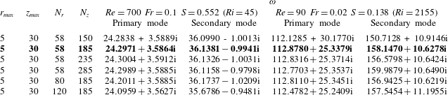
B.4 Numerical solution to EVP
After discretizing the differential operators in (2.15) and imposing boundary conditions as per
 $m$
, the generalized EVP can be expressed as a set of linear algebraic equations as
 $$\begin{eqnarray}{\mathcal{A}}\hat{q}=\unicode[STIX]{x1D714}{\mathcal{B}}\hat{q},\end{eqnarray}$$
where
 ${\mathcal{A}}$
and
 ${\mathcal{B}}$
are matrices of size
 $5N_{r}N_{z}\times 5N_{r}N_{z}$
that correspond to discretized versions of differential operators
 $\unicode[STIX]{x1D63C}$
and
 $\unicode[STIX]{x1D63D}$
in (2.15) along with boundary conditions. The application of the QZ algorithm for recovering the full eigenspectrum is not feasible since an accurate numerical solution of the global linear stability problem requires mesh sizes as shown in table 3 which leads to larger matrix sizes i.e.
 $O(10^{4}-10^{5})\times O(10^{4}-10^{5})$
. So, an iterative Arnoldi method is used in the present study which is widely employed and the most successful approach for numerical solution of a large-scale EVP (Juniper et al.
Reference Juniper, Hanifi and Theofilis2014). The generalized EVP is converted to a standard EVP by employing a shift and invert strategy, with
 $\unicode[STIX]{x1D706}$
as shift parameter as
 $$\begin{eqnarray}{\mathcal{M}}\hat{q}={\displaystyle \frac{1}{\unicode[STIX]{x1D714}-\unicode[STIX]{x1D706}}}\hat{q}\quad \text{where, }{\mathcal{M}}=({\mathcal{A}}-\unicode[STIX]{x1D706}{\mathcal{B}})^{-1}{\mathcal{B}}.\end{eqnarray}$$
Using this method, instead of resolving the entire spectrum which requires greater computational resources and time, the least stable part of the spectrum is calculated by recovering a set of eigenvalues of largest magnitude in the vicinity of shift parameter
 $\unicode[STIX]{x1D706}$
. A set of 200 eigenvalues of larger magnitude along with the corresponding eigenvectors are recovered for each case.
B.5 Mesh and domain dependence study for global instability computations
For performing the instability analysis (2.15), a mesh size of
 $(N_{r},N_{z})=(58,185)$
and domain size of
 $(r_{max},z_{max})=(5,30)$
have been chosen after performing a mesh and domain dependence study. This study has been done for two randomly selected cases namely, 1.
 $Re=700$
,
 $Fr=0.1$
,
 $S=0.552$
(
 $Ri=45$
) and 2.
 $Re=90$
,
 $Fr=0.02$
,
 $S=0.138$
(
 $Ri=2155$
), one at lower
 $Ri$
and the other at higher
 $Ri$
. The global eigenvalue spectrum shows two discrete modes (i.e. primary and secondary modes, refer § 4.2.1) for these cases. The global frequency (
 $\unicode[STIX]{x1D714}_{r}$
) and growth rates (
 $\unicode[STIX]{x1D714}_{i}$
) of these two discrete modes obtained for various domain and mesh sizes are listed in tables 2 and 3 respectively for comparison. From these results, we found that for mesh size
 $(N_{r},N_{z})=(58,185)$
and domain size
 $(r_{max},z_{max})=(5,30)$
, the unstable modes achieved reasonable convergence for both cases and for both modes. Hence, these mesh parameters are used for all the cases discussed in the present work.
Appendix C. Stability computations for realistic velocity profiles that arise from finite length pipe nozzles
To complement our investigation regarding the effect of the inlet velocity profile on plume instability (refer § 4.4), we further carried out global stability computations for base flows obtained using realistic inlet velocity profiles that correspond to pipe nozzles of various lengths. For this investigation, we followed an approach similar to that of Coenen, Sevilla & Sánchez (Reference Coenen, Sevilla and Sánchez2008) and is briefly described here. Firstly, the velocity profiles that arise at the outlet of the pipe nozzles of various non-dimensional lengths
 ${\mathcal{L}}=L/D$
are computed. The schematic of the pipe-nozzle domain, used for the computation of these outlet velocity profiles, is presented in figure 28(a). The outlet velocity profiles thus obtained for a typical plume case
 $Re=150$
,
 $Fr=0.04$
and
 $S=0.138$
(
 $Ri=539$
) for various
 ${\mathcal{L}}$
are presented in figure 28(b). Note that the outlet velocity profiles vary from plug flow to parabolic shape with an increase in
 ${\mathcal{L}}$
as shown in figure 28(b).
(a) Schematic of a pipe nozzle and, (b) velocity profiles computed at the exit of the pipe nozzles of different length-to-diameter
 ${\mathcal{L}}$
ratios.

Schematic of the axisymmetric domain chosen for base flow computations to simulate plumes emanating from pipe nozzles.

Each outlet velocity profile thus obtained for a fixed
 ${\mathcal{L}}$
is then given as inlet boundary condition to the plume as shown in figure 29 and the corresponding plume base flow has been computed. In figure 29, while the inlet velocity profile depends on
 ${\mathcal{L}}$
, the inlet mass fraction is kept constant. The computed base flow for each
 ${\mathcal{L}}$
is then used for performing global linear stability analysis. This analysis has been performed for two
 $Ri$
values,
 $Ri=199$
and 539.
Eigenvalue spectra for two plume cases (a)
 $Re=150$
,
 $Fr=0.04$
and
 $S=0.138$
(
 $Ri=539$
) and (b)
 $Re=200$
,
 $Fr=0.066$
and
 $S=0.138$
(
 $Ri=199$
), obtained for finite length nozzles of different length-to-diameter ratios (
 ${\mathcal{L}}$
).


The global eigenvalue spectra thus obtained for
 $Ri=539$
and
 $Ri=199$
are shown in figures 30(a) and 30(b) respectively. These figures show that the primary mode attains larger growth rates than the secondary mode for pipes of all
 ${\mathcal{L}}$
. Also, it can be observed that the complex frequency
 $\unicode[STIX]{x1D714}$
saturates to a constant value with increase in
 ${\mathcal{L}}$
, as the inlet velocity profile tends to attain parabolic shape at larger
 ${\mathcal{L}}$
.
The Strouhal numbers of the two unstable modes in 30(a) and 30(b) are plotted in figure 31 as a function of their corresponding Richardson numbers. Additionally, the
 $St{-}Ri$
scaling laws of the primary mode (solid line) and the secondary mode (dashed line) obtained for the tanh velocity profile with
 $R/\unicode[STIX]{x1D703}_{v}=100$
in figure 12, and the
 $St{-}Ri$
scaling law of the primary mode (dash-dot line) obtained for parabolic inlet velocity profile in figure 24, are also shown in figure 31 for comparison.
The
 $St$
of both primary and secondary modes for
 ${\mathcal{L}}=0$
(i.e. uniform velocity profile) are in good agreement with their respective
 $St{-}Ri$
scaling laws, obtained for tanh velocity profile with
 $R/\unicode[STIX]{x1D703}_{v}=100$
. With an increase in
 ${\mathcal{L}}$
, the
 $St$
values increase marginally, and saturate to the
 $St{-}Ri$
scaling of parabolic velocity profile as observed in figure 31.
More importantly, the analysis presented here, coupled with our experiments using pipe nozzles (figure 21 b) unambiguously proves that the difference in inlet conditions between the present global stability analysis and the experiments of Cetegen & Kasper (Reference Cetegen and Kasper1996) is not the reason for the earlier switch in frequency scaling.