





1. Introduction
The goal of this work is to examine how well physics-informed neural networks (PINNs) can solve nonlinear partial differential equations (PDEs). In particular, we are interested in whether a PINN can capture genuinely nonlinear behaviour, such as the soliton interactions studied here, when that behaviour is never directly supplied to the network, and in characterizing how reliably it does so as the complexity of the underlying solution increases. We focus on a class of equations that are well studied analytically and primarily used for modelling water waves in both two and three dimensions – the Korteweg–de Vries (KdV) and the Kadomtsev–Petviashvili (KP) equations. In particular, we study how well PINNs can find soliton solutions to these nonlinear, dispersive PDEs. Solitons propagate without changing shape, by balancing nonlinearity and dispersion. After their nonlinear interaction, they emerge from collisions unchanged except for a possible phase shift. Thus, a numerical solver can only be considered effective if it accurately captures this characteristic behaviour. Aside from KP and KdV’s modelling applications, they are completely integrable and exactly solvable [Reference Mulase42], which implies that they admit well-behaved solutions.
It is well known that PDEs are hard to solve both numerically and analytically in all generality, in particular if they are nonlinear. The benefit of focusing on KdV and KP and their soliton solutions is that these are well-studied equations with available analytical solutions. There are various methods for finding soliton solutions for KdV and KP, such as the inverse scattering transform [Reference Ablowitz and Clarkson2, Reference Ablowitz, Yaacov and Fokas4, Reference Fokas and Ablowitz15, Reference Gardner, Greene, Kruskal and Miura17, Reference Gardner, Greene, Kruskal and Miura18, Reference Manakov and Zakharov38], Riemann–Hilbert methods [Reference Novikov, Manakov, Pitaevskii and Zakharov45] and the Darboux transforms [Reference Matveev and Salle40], just to name a few. In this work, we use the form of solutions given by Hirota [Reference Hirota23–Reference Hirota and Miura25, Reference Satsuma49] for comparison to the numerical results we obtain from PINNs, as this method easily adapts to  $N$-soliton solutions.
It is important to note that solutions to KdV and KP have also been found numerically. Historically, finite difference schemes were the first to be used, going back to Zabusky and Kruskal’s original study of KdV solitons [Reference Zabusky and Kruskal57]. Such schemes remain a natural choice for lower-order or more general equations, but for KdV and KP specifically they are typically outperformed by pseudospectral (Fourier) methods, which exploit the fact that the linear dispersive terms in both equations are diagonal in Fourier space. The benchmark comparative study of Taha and Ablowitz [Reference Taha and Ablowitz51] established this directly for KdV, showing that pseudospectral schemes reach a given accuracy substantially faster than finite differences for the one- and two-soliton problem, and pseudospectral or split-step Fourier integration has since become the standard approach for this class of equations.
The KP equation poses an additional complication for classical solvers, since its line-soliton solutions are not spatially localized and instead extend to the boundary of any finite computational domain [Reference Biondini, Maruno, Oikawa and Tsuji8]. Ablowitz and Baldwin [Reference Ablowitz and Baldwin1], whose analytic line-soliton solutions we use to define our own initial and boundary data, report X- and Y-type line-soliton interactions as a naturally occurring phenomenon on shallow beaches and give closed-form Hirota solutions for them, but do not address this numerical boundary treatment. Kao and Kodama [Reference Kao and Kodama30] instead address it with a windowing method, which smoothly damps the solution near the transverse domain boundaries so that a standard Fourier pseudospectral discretization can be used, with the true line-soliton solution recovered outside the windowed region. This approach achieves high (spectral) accuracy once the windowing scheme is in place, but requires this equation-specific boundary treatment, in contrast to the mesh-free approach used here, where the boundary is instead enforced directly as a labelled loss term. PINNs themselves have since been compared directly against classical solvers [Reference Bai, Koley, Mishra and Molinaro6, Reference Haight, Roudenko and Wang21, Reference Ortiz, Marín and Ortiz46], generally finding that classical methods remain faster and more accurate for problems with fully known initial and boundary data, though often requiring exactly this kind of equation-specific discretization choice that a mesh-free method does not need. We return to a quantitative comparison between our own PINN results and these classical benchmarks in Section 4.
More recently, PINNs have emerged as a method to find solutions to PDEs [Reference Raissi, Perdikaris and Karniadakis47], which relies on the property of feedforward neural networks being universal function approximators [Reference Dissanayake and Phan-Thien13, Reference Hornik, Stinchcombe and White26]. One of the first prominent works to apply PINNs to the KdV equation was [Reference Raissi, Perdikaris and Karniadakis47], who proposed using neural networks to solve forward and inverse problems involving nonlinear PDEs. PINNs are different from conventional neural networks as they incorporate physical laws, in the form of PDEs, in their loss function. This allows for a reduction in the number of labelled training examples needed, which traditional neural networks require. Furthermore, traditional neural networks learn by being given exact input and output pairs to the network (i.e. supervised learning), but using the PDE in the loss allows the network to learn the solution within the problem domain without knowing the exact solution for the training points. In practice, the governing equation constrains the solution space to those that are admitted by the PDE, while the initial conditions (ICs) and boundary conditions (BCs) appear as supervised loss terms, ensuring the solution is unique. In their work, they illustrated how a PINN could approximate solutions to the nonlinear Schrödinger equation with periodic BCs, as well as the Allen–Cahn and KdV equations. They also considered the inverse problem of finding the PDEs from data, illustrating how this would work for Navier–Stokes and KdV, by analysing how well the PINN can find the parameters in the PDE.
Since then, the optimization procedure for finding soliton solutions to KdV and modified KdV equations has been refined [Reference Li, Chen and Li35] by balancing the different terms in the loss function to avoid oscillations in the gradients. For consideration of solitary wave solutions to the mKdV equation and the improved Boussinesq equation, hyperparameters were introduced to speed up the optimization procedure, resulting in more accurate solutions in [Reference Guo, Cao and Peng20]. Higher-dimensional PDEs such as the KP equation have been explored using PINNs to find breather and lump solutions, among others [Reference Miao and Chen41]. For a full review of PINNs as applied to fluid dynamics, see [Reference Zhao, Zhang, Lou, Wang and Yang58], and for a more comprehensive review of PINNs, see [Reference Toscano, Oommen, Varghese, Zou, Daryakenari, Wu and Karniadakis52].
In this work, we carry out a systematic study of how PINN performance scales with the complexity of the KdV and KP soliton solutions being approximated, and of how this performance depends on the choices involved in training. We train and evaluate PINNs across an increasing number of interacting solitons for KdV, from one soliton up to three, and analogous line-soliton junction configurations for KP, including a three-line-soliton ‘2-in-3-out’ junction, quantifying accuracy, training time and required network architecture in each case (Section 4). Throughout, the IC supplied to the network never encodes the nonlinear soliton interaction itself, as it consists only of the individual, single-soliton profiles (equation (2.5)) that make up the solution, placed far enough apart (within some numerical tolerance) that they do not yet interact. The PINN must therefore recover the full nonlinear interaction and phase shifts encoded in the coefficients  $A_{ij}$ of equation (2.4) from the governing PDE alone. This flexibility means the same PINN framework can be adapted across different ICs, recovering a full multi-soliton interaction from initial data describing only individual, well-separated solitons. However, we find that the network architecture and training strategy required to do so reliably are not obvious in advance, and become increasingly demanding as the number of interacting solitons grows, a point we return to in Section 3.
The paper is laid out as follows. First, we describe the equations and particular types of solutions that we are considering in Section 2. We then describe the neural network architecture we use for the optimization problem of minimizing the given loss, as well as the chosen hyperparameters in Section 3. We finish by presenting the types of one- and two-soliton solutions for both the KdV and KP equations in Section 4, and conclude our findings and comment on the performance of PINNs in Section 5.
2. Mathematical formulation
The KdV equation is a well-studied model for inviscid surface waves in shallow water in one dimension, first proposed by Boussinesq in 1872 [Reference Boussinesq10], then Korteweg and de Vries in 1895 [Reference Korteweg and de Vries33]. In non-dimensional form, it is given by
 \begin{equation}
u_t + 6 uu_x + u_{xxx} = 0,
\end{equation}
where  $u(x,t)$ is the vertical displacement from equilibrium,
 $(x,t)$ are spatial and time variables, and subscripts denote partial derivatives. The scenario is depicted in Figure 1. This equation includes both a nonlinear and a dispersive term, and admits soliton solutions [Reference Ablowitz and Clarkson2, Reference Drazin and Johnson14, Reference Strutt48]. The solitary profiles interact nonlinearly and emerge unchanged, except for a phase shift, and it is due to this particle-like behaviour that they are often referred to as solitons [Reference Zabusky and Kruskal57]. It is known that KdV is integrable and exhibits
 $N$-soliton solutions [Reference Gardner, Greene, Kruskal and Miura17, Reference Lax34].
 $u(x,t)$ denotes the surface of the wave from its undisturbed level at
 $u=0$ with depth
 $h$.

The KdV equation (2.1) can be extended to capture two-dimensional, small-amplitude waves in shallow water by considering the KP equation. It was first used by Kadomtsev and Petviashvili in 1970 when they investigated the stability of the KdV soliton with transverse perturbations [Reference Kadomtsev and Petviashvili29]. This equation was also derived in the context of water waves by considering the motion of irrotational, inviscid and incompressible fluid, assuming small-amplitude waves and shallow water where the motion is primarily one-dimensional [Reference Ablowitz and Clarkson2, Reference Ablowitz and Segur3, Reference Stokes50]. The non-dimensional KP equation is given by
 \begin{equation}
(u_t + 6uu_x + u_{xxx})_x + 3 \sigma u_{yy} = 0, \ \text{with} \ \sigma =\pm 1,
\end{equation}
where the subscripts denote partial derivatives and the displacement from equilibrium is denoted by  $u(x,y,t)$ with the spatial variables
 $(x,y)$ and time
 $t$. The parameter
 $\sigma$ can take on values of
 $\pm 1$. When
 $\sigma = -1$, equation (2.2) is referred to as KPI, and when
 $\sigma = 1$, it is KPII. For this work, we focus on soliton solutions of KPII, as this is the regime of weak surface tension, which is valid for waves in the ocean and, in our opinion, a more interesting regime to examine using PINNs due to its practical applications. It is notable that every solution to the KdV is also a solution to KPII. It has also been shown that KPII has
 $N$-line-soliton solutions, wherein the
 $N$ solitons travel in different directions and interact obliquely [Reference Satsuma49].
There are many ways to write the soliton solutions; we focus on the Hirota notation [Reference Ablowitz and Baldwin1, Reference Hietarinta, Kosmann-Schwarzbach, Grammaticos and Tamizhmani22, Reference Hirota23], where the solution can be represented as
 \begin{equation}
u = 2 \frac{\partial^2}{\partial x^2} \ln (F^{(N)})
\end{equation}
with
 \begin{equation}
F^{(N)} = \sum_{\mu_i} \exp \left(\sum_{i=1}^N \mu_i \eta_i+\sum_{i \lt j}^{N} \mu_i \mu_j a_{ij} \right)
\end{equation}
where  $N$ denotes the number of solitons and
 $\mu_i \in \{0,1\}$ for
 $i,j \in \{1, \ldots, N\}$
 \begin{align*}
\eta_i &= k_i x - k_i^3 t + \delta_{i} \ & \text{for KdV}, \\
\eta_i &= k_i \left( x + P_i y - (k_i^2+3\sigma P_i^2)t\right) + \delta_i \ & \text{for KP}
\end{align*}
and  $a_{ij} = \ln{(A_{ij})}$, where
 $i \lt j$ with
 \begin{align*}
A_{ij} &= \frac{(k_i - k_j)^2}{(k_i +k_j)^2} & \text{for KdV}, \\
A_{ij} & = \frac{(k_i-k_j)^2 - \sigma (P_i-P_j)^2}{(k_i+k_j)^2 - \sigma (P_i-P_j)^2}, & \text{for KP}.
\end{align*}
if we consider  $k, \lambda$ to be the wavenumbers in
 $x$ and
 $y$, respectively, where for convenience we have introduced
 $P = \lambda/k$ [Reference Ablowitz and Baldwin1]. Moreover,
 $\delta_i$ is a constant denoting the phase shift, with
 $x,y$ and
 $t$ representing the spatial and temporal variables, respectively.
In this work, we focus on one- and two-soliton solutions to KdV and KP, which take the same form but differ in the number of spatial dimensions. More explicitly, the one-soliton solutions are given by (2.3) with
 \begin{align}F^{(1)} & = \sum_{\mu_1 \in\{0,1\}} e^{\mu_1 \eta_1} \nonumber
\\ & = 1 + e^{\eta_1}.\end{align}
We can simplify this in the case of KdV to be
 \begin{align*}
u^{(1)}_{\text{KdV}} = \frac{k^2}{2} \text{sech}^2 \left( \frac{\eta_1}{2} \right).
\end{align*}
In this form, it is easy to see that
 \begin{align*}
c = k^2 \ \ \text{and} \ \ A = \frac{c}{2}
\end{align*}
where  $c$ is the phase speed, and
 $A$ is the amplitude of the soliton. Observe that the speed of individual solitons is proportional to
 $A$, with larger amplitude waves travelling faster. For the two-soliton solution, after enumerating over all possible combinations of
 $\mu_1, \mu_2 \in \{0,1\}$, we obtain
 \begin{align}F^{(2)} & = \sum_{\mu_1, \mu_2 \in\{0,1\}} e^{\mu_1 \eta_1+\mu_2 \eta_2+\mu_1 \mu_2 a_{12}} \nonumber \\
& = 1 + e^{\eta_1} + e^{\eta_2} + A_{12}e^{\eta_1+\eta_2}.\end{align}
It is important to note that the analytical form of the solution is only used to define the IC and, in the case of PINNs for the KP equation, boundary data. Otherwise, the PINN is not aware of the analytical solution for any other points in the domain, as explained further in Section 3. The only other way the analytical solution is used is to compute the accuracy of the PINN-predicted solution, i.e. in the error analysis. We also note that we visualize the effects of nonlinearity for the KdV two-soliton solution by comparing the linear combination of single soliton solutions to the two-soliton PINN-predicted solution. When doing these comparisons, in order to make sure we overlay the analogous solitons prior to their interaction, we need to apply phase shifts. We shift each soliton of the linear combination by
 \begin{equation}
\delta_1 = 0
\end{equation}
 \begin{equation}
\delta_2 = a_{12} = 2 \ln \left(\frac{k_1 - k_2}{k_1 + k_2}\right).
\end{equation}
Observe that only the smaller (slower) soliton needs a shift.
3. Physics-informed neural networks (PINNs)
The main goal of this work is to observe if PINNs can accurately find nonlinear and dispersive soliton solutions to well-understood KdV and KP equations ((2.1) and (2.2)) corresponding to analytical solutions given by equation (2.3). We use the implementation presented in [Reference Raissi, Perdikaris and Karniadakis47] and employ a deep, fully connected feedforward neural network. Computing solutions involves initializing, training and then using a PINN.
The network is comprised of input, hidden and output layers, which in turn are made up of neurons (or nodes). In the case of the KdV equation, the input layer is composed of two nodes which correspond to its independent variables  $(x,t)$. In the KP case, we add an additional node such that there are three nodes, which correspond to
 $(x,y,t)$. The output node represents the PINN-predicted solution
 $u_{\text{PINN}}(x,y,t)$. The layers are fully connected in a feedforward way, with connections between layers parameterized by weights and biases, which we collectively refer to as trainable parameters
 $\theta$.
The hyperbolic tangent activation function is applied to layer outputs prior to passing them to a following layer. We compare this choice against seven alternative activation functions in Appendix D, where tanh is shown to reach comparable accuracy to the best-performing alternatives at substantially lower training cost.
We can consider the PINN as a multitask learner with the objective of simultaneously learning the data, composed of particular ICs and BCs, while also satisfying the PDE. We define the set of points used for training as
 \begin{align*}
\mathcal{X}_{\text{train}} = \mathcal{X}_{\text{IC}} \cup \mathcal{X}_{\text{BC}} \cup \mathcal{X}_{\text{PDE}} = \{\mathbf{x}^{1}, \mathbf{x}^{2}, \ldots, \mathbf{x}^{N}\}
\end{align*}
consisting of points  $\mathbf{x}^{i} = \{x^i, y^i, t^i\}$, where
 $x^i$,
 $y^i$ and
 $t^i$ are drawn from a given distribution, and
 $i$ denotes the training sample. Note that the training set
 $\mathcal{X}_\text{train}$ is composed of disjoint sets
 $\mathcal{X}_{\text{IC}}$,
 $\mathcal{X}_{\text{BC}}$, which have associated solution data (labels), and
 $\mathcal{X}_{\text{PDE}}$ denoting points which are used to compute the PDE residual, defined as the left-hand side of equation (2.2). Hereafter, we refer to these data as initial, boundary and collocation points, respectively.
We define the training objective as a minimization of the total loss  $L$, which is given by the weighted sum
 \begin{equation}
L(\theta, \mathcal{X}) = w_{\text{IC}} L_{\text{IC}}(\theta, \mathcal{X}_{\text{IC}}) + w_{\text{BC}} L_{\text{BC}}(\theta, \mathcal{X}_{\text{BC}}) + w_{\text{PDE}} L_{\text{PDE}}(\theta, \mathcal{X}_{\text{PDE}}),
\end{equation}
where  $w_m$ are the loss weights (not to be confused with a trainable parameter), and
 $L_m$ is the loss of a particular task, defined to be the mean squared error given as
 \begin{align*}
L_{\text{BC}} & = \frac{1}{N_{\text{BC}}} \sum_{i=1}^{N_\text{BC}} |u_{\text{exact}}(\mathbf{x}^i_\text{BC})-\hat{u}_{\text{PINN}}^i|^2, \\
L_{\text{IC}} & = \frac{1}{N_{\text{IC}}} \sum_{j=1}^{N_{\text{IC}}} |u_{\text{exact}}(\mathbf{x}^j_\text{IC})-\hat{u}_{\text{PINN}}^j|^2, \\
L_{\text{PDE}} & = \frac{1}{N_{\text{PDE}}} \sum_{k=1}^{N_{\text{PDE}}} |f_{\text{exact}}(\mathbf{x}_{\text{PDE}}^k) - \hat{f}_{\text{PINN}}(\mathbf{x}_{\text{PDE}}^k)|^2.
\end{align*}
Training the PINN involves finding the optimal parameters  $\theta$ which minimize the total loss
 $L$. This is done using a set of optimizers, for a particular training set
 $\mathcal{X}_{\text{train}}$. The number of training samples is denoted as
 $N_{\text{BC}}$,
 $N_{\text{IC}}$ and
 $N_{\text{PDE}}$ for the BC, IC and collocation points. We denote
 $u_{\text{exact}}$ as the exact solution evaluated on initial and boundary points, and
 $\hat{u}_{\text{PINN}}$ denotes the PINN’s output value given the corresponding input points. Finally,
 $f_{\text{exact}}$ is the right-hand side of the PDE, either equation (2.1) or (2.2), which in our case is trivial (
 $f_{\text{exact}} := 0$). Given that the BC and IC are prescribed, this corresponds to having labelled data, in contrast to the interior points which are not labelled.
Training data for the IC and BC are evenly spaced, and domain points are sampled from a uniform distribution. In this instance-based approach, treating  $u(x,y,t)$ as a scalar dependent on a set of values within the domain implies that the PDE is satisfied pointwise. In addition, we can evaluate the model by comparing the PINN prediction to the analytical solution on a set of test points, which may differ from the training points. In this way, the PINN solution is mesh–free, which is greatly advantageous.
Computing these solutions involves initializing a PINN, and then training it with a particular training set  $\mathcal{X}_\text{train}$ to obtain optimal parameters
 $\theta$, followed by using it on a test set
 $\mathcal{X}_\text{train}$. The overall procedure is shown in Algorithm 1. The parameters
 $\theta$ of the network were initialized using the Xavier normal distribution [Reference Glorot and Bengio19]. For the beginning stages (1000 epochs) [Reference Lu, Meng, Mao and Karniadakis37], the algorithm used to minimize the loss term was the Adam (Adaptive Moment Estimation) optimizer relying on stochastic gradient descent [Reference Kingma and Ba32]. To refine the training, the L-BFGS (limited-memory Broyden–Fletcher–Goldfarb–Shanno) algorithm was used in later stages [Reference Matthies and Strang39, Reference Nocedal43], which is a quasi-Newton method relying on the Jacobian and a pseudo-inverse of the Hessian to optimize.
Adam and L-BFGS have complementary strengths that motivate using them in sequence rather than either one alone. Adam [Reference Kingma and Ba32] is a first-order, stochastic, adaptive-learning-rate method and comparatively cheaper per iteration, robust to the highly non-convex and initially noisy loss landscape typical of PINN training, and is generally not prone to becoming trapped in shallow local minima or saddle points early on. Its drawback is that it converges slowly once close to a minimum, and typically stalls at a relatively high loss value even after many epochs. L-BFGS [Reference Matthies and Strang39, Reference Nocedal43] is instead a quasi-Newton, second-order method that builds an approximation of the inverse Hessian from recent gradient history, and it converges much faster, but each iteration is more expensive, it is more sensitive to the quality of the starting point, and it can perform poorly or fail to make progress on the noisy, highly oscillatory loss surfaces that PDE residual terms typically produce early in training. Using L-BFGS alone from a random initialization is therefore prone to stalling in a poor local minimum before the optimizer ever reaches the basin in which its fast convergence properties are useful. The two-stage schedule used throughout this work with Adam for the first 1000 epochs, followed by L-BFGS until convergence, follows the original PINN formulation of [Reference Raissi, Perdikaris and Karniadakis47] and is now standard practice in the PINN literature. It is intended to combine Adam’s early robustness with L-BFGS’s fast late-stage refinement.

4. Results
In this section, we present the PINN-approximated solutions for the KdV and KP equations, (2.1) and (2.2), respectively. All computations were performed using Python with PyTorch 2.5 on an NVIDIA GeForce RTX 4090 GPU using CUDA 12.4. The collocation points were sampled randomly, and data for the IC and BC were sampled evenly. Finding particular  $N$-soliton solutions involves training a PINN with the corresponding IC and BC for the case of interest. The parameters for the ICs are given in Table 1 and were obtained from [Reference Anco and Willoughby5] for KdV or [Reference Ablowitz and Baldwin1] for KP in order to match well-understood results. We note that the ICs for the two-soliton solution for KdV are given by a superposition of two separate one-soliton solutions (2.5) with the phase
 $\delta_i$ computed using (2.7), representing two solitons far enough apart such that the interaction term is negligible. In all other cases, the phases for ICs are set to zero. For KP, the IC is such that the interaction of the line solitons is outside of the computational domain. This is done to see if the PINN can capture the nonlinearity without it being explicitly given.
Parameters used for ICs

Table 1 Long description
Parameters are listed for initial conditions across two models, KdV and KP, each split into soliton cases. Columns are KdV 1 soliton, KdV 2 soliton, KP 1 soliton, KP 2 soliton X, and KP 2 soliton Y. Under x direction, k1 is 0.9 for KdV 1 soliton and 1.0 for KdV 2 soliton, while k1 is one half for all three KP columns. Under x direction, k2 is not given for KdV 1 soliton, is the square root of 1.2 divided by 4 for KdV 2 soliton, is not given for KP 1 soliton, and is one half for KP 2 soliton X and 1.0 for KP 2 soliton Y. Under y direction, P1 and P2 are not given for either KdV column. Under y direction for KP, P1 is two thirds for KP 1 soliton, negative two thirds for KP 2 soliton X, and three quarters for KP 2 soliton Y. Under y direction for KP, P2 is not given for KP 1 soliton, is two thirds for KP 2 soliton X, and one quarter for KP 2 soliton Y.
The set of parameters used in the optimization procedure is given in Table 2. Note that automatic differentiation [Reference Baydin, Pearlmutter, Radul and Siskind7] is used, as implemented in PyTorch, to compute loss gradients and the derivatives appearing in the KdV and KP equations (2.1) and (2.2). Once the network is trained, the solution is examined on a test set of uniformly generated  $N_{\text{test}}= 1\times 10^6$ points
 $\mathcal{X}_{\text{test}}$, which do not necessarily correspond to the training set. The point-wise normalized absolute error between the PINN predicted solution
 $\hat{u}_{\text{PINN}}$ and the exact solution
 ${u}_{\text{exact}}$ given by (2.3) with (2.4) is computed by
 \begin{equation}
e_l = \frac{|{u_{\text{exact}}(\mathbf x^l) - \hat{u}_{\text{PINN}}(\mathbf{x}^l)}|}{\max\limits_{\mathbf{x} \in \mathcal{X}_\text{test}}{|{u_{\text{exact}}(\mathbf{x}^l)}|}},
\end{equation}
where  $l = 1, 2, \ldots, N_\text{test}$. We often report the maximum point-wise normalized absolute error, which we denote by
 $||e||_\infty = \max\limits_{1 \leq l \leq N_\text{test}} (e_l)$. This was chosen because (4.1) gave the best measure of how accurately we captured the soliton solutions.
Optimizer parameters used, common to all training cases and runs

Table 2 Long description
Parameters and values are listed for two optimizers, Adam and L B F G S. Under Adam, learning rate is one times ten to the minus three, and number of epochs is 1000. Under L B F G S, learning rate is 1.0. L B F G S also lists max iterations as five times ten to the fourth and max evaluations as one times ten to the fifth. Tolerance, grad is one times ten to the minus eight, and tolerance, change is one times ten to the minus sixteen. History size is 300, and line search method is Strong Wolfe.
The architecture of the PINN, the number of points used in the training sets, as well as the weights for each term in the loss function (3.1) for the cases we considered, are summarized in Table 3. The architecture (number of layers and neurons per layer) for the KdV cases was chosen based on the architecture which gave the lowest final loss among those tested, from the results as given in Appendix A. From this table, we see that the number of neurons and layers increases as the number of solitons increases in the case of KdV where the BCs are trivial (zero). On the contrary, these hyperparameters do not change for the case of KP line solitons interacting, resulting in x or y junctions because the complexity of those solutions is relatively similar to each other, and the BCs are prescribed exactly, but the number of layers does increase between one- and two-soliton solutions. The loss weight ( $w_{BC}$) for the zero BCs for KdV is less important and is set to be smaller relative to other weights than in the case of KPII, where the BCs are nontrivial (see Appendix B for loss histories separated according to BC, IC and PDE components). The maximum error (equation (4.1)), the final training loss (using equation (3.1)) and the time it takes to train one instance of the PINN for each scenario considered in this work are summarized in Table 4. From this table, we see the PINN optimizes the loss to a small tolerance (at least
 $1\times 10^{-6}$) in minutes. However, the maximum error increases as the number of solitons increases for KdV, where the BCs are trivially zero, as this part of the loss term does not contribute as much as the equivalent in the line soliton case of KPII.
A summary of architecture size, training data counts and loss weights used for PINNs trained to solve the KdV and KP equations for various solution cases

Table 3 Long description
Rows list cases for KdV and KP, with columns for architecture, training data counts, and loss weights. Architecture is given as neurons and layers, training data as N BC, N IC, and N PDE, and loss weights as w BC, w IC, and w PDE. For KdV 1 soliton, neurons 16 and layers 4, with N BC 10,000, N IC 30,000, N PDE 50,000, and weights 1.0, 5.0, and 15.0 for BC, IC, and PDE. For KdV 2 soliton, neurons 62 and layers 7, with N BC 10,000, N IC 10,000, N PDE 100,000, and weights 1.0, 10.0, and 100.0. For KP 1 soliton, neurons 32 and layers 3, with N BC 10,000, N IC 10,000, N PDE 50,000, and weights 1.0, 1.0, and 10.0. For KP x junction, neurons 32 and layers 8, with the same training data counts and weights as KP 1 soliton. For KP y junction, neurons 32 and layers 8, again with N BC 10,000, N IC 10,000, N PDE 50,000, and weights 1.0, 1.0, and 10.0.
Notes: We see that the number of neurons and layers increases when going from one to two solitons in the case of KdV, but does not change depending on the junction type for KP, as expected.
A summary of the performance (max normalized absolute error  $||e||_\infty$, final training loss and training time) of PINNs, trained and tested for various solution cases of the KdV and KP equations

Table 4 Long description
Performance is reported by case using three measures: maximum normalized absolute error, final loss, and time in minutes and seconds. For KdV 1-soliton, the maximum error is 2.92 times 10 to the minus 3, final loss is 1.08 times 10 to the minus 7, and time is 00:20. For KdV 2-soliton, the maximum error is 1.02 times 10 to the minus 1, final loss is 4.48 times 10 to the minus 7, and time is 10:39. For KP 1-soliton, the maximum error is 2.74 times 10 to the minus 2, final loss is 6.61 times 10 to the minus 8, and time is 02:58. For KP x-junction, the maximum error is 1.55 times 10 to the minus 2, final loss is 2.31 times 10 to the minus 7, and time is 03:57. For KP y-junction, the maximum error is 1.59 times 10 to the minus 2, final loss is 1.14 times 10 to the minus 6, and time is 03:02.
Notes: We see the PINN optimizes the loss to a small tolerance (at least  $1\times 10^{-6}$) in a relatively short amount of time (min). However, the maximum error increases for the case of KdV as we go from one to two solitons.
The solutions that were found by the PINN were examined using  $N_\text{test} = 1\times 10^6$ test set of points evenly sampled from the domain. For the KdV, these solutions are shown in Figure 2 for the one-soliton case and Figure 6 for the two-soliton case. From both of these cases, we can see the solitons travel at a constant speed while maintaining their shape and amplitude, except during the nonlinear interaction depicted in Figure 6. When compared with a superposition of two single solitons, depicted by the dashed blue lines in the same figure, it can be seen that the interaction is truly nonlinear and that the solitons emerge from the interaction with only a change in phase.
Solutions to the KdV equation for the single-soliton IC computed by a PINN over a test set of points within the training domain. Plots (top to bottom) show profiles at the initial, middle and final training time. The soliton is seen travelling at a constant speed while maintaining its shape, as expected.

The training loss given by equation 3.1 that was optimized for the case of one- and two-soliton ICs of the KdV equation is shown in Figures 3 and 7, where the blue line shows the training history of the PINN that computes the particular solutions we show in this work, with the black solid line representing the mean and grey region representing the 0.02–0.98 inter-quantile range for 100 training runs (replications). Note that the plots are truncated to that of the shortest training run, with the full component-wise loss histories shown in Appendix B, in Figure B1. The variance in training runs is explained due to having a random initialization of the network’s trainable weights and biases, and the set of collocation points chosen randomly within the domain. The dashed vertical line represents where the optimizer was switched from Adam to L-BFGS. As can be seen, in particular from the training loss for the KdV two-soliton case, when using the Adam optimizer, the loss tends to oscillate, suggesting the optimizer keeps missing the direction of the smallest gradient. While it may be possible to adjust the learning rates or other parameters to prevent this from happening, when switching to the L-BFGS, this oscillatory behaviour is no longer seen, and the optimizer performs better at finding a path to a minimum of the total loss.
Total loss during training of a PINN that solves the KdV equation for the single soliton IC. The blue solid line shows the training history of the PINN giving solutions seen in Figure 2; the black solid line represents the mean, with the grey region representing the 0.02–0.98 inter-quantile range. The dashed vertical line represents where the optimizer was switched from Adam to L-BFGS.

When comparing the PINN-predicted solutions to KdV to the analytic solutions using (4.1), we see from Table 4 that the maximum normalized error for one soliton is  $2.92 \times 10^{-3}$ and for two solitons is
 $1.02\times10^{-1}$, with Figure 5 and Figure 8 showing in more detail in which region these errors are largest. These figures depict the mean error averaged over
 $t$ (top) or
 $x$ (bottom), with the grey region again representing the 0.02–0.98 inter-quantile range for 100 training runs (replications), with the black line representing the mean and the blue line representing the particular solutions we examined. As expected, since the ICs and the BCs are in the loss function, the error in these regions is smallest. Figures 4 and 9 show the space-time portrait of the KdV one- and two-soliton solutions on the left, with the log of the normalized error for 100 training runs (replications) on the right. It can be seen that the PINN solution captures the amplitude of the solitons and the constant speed, but the largest error is at the furthest time examined, with the PINN not capturing the shape of the largest solitons as well.
Space-time portraits of the one-soliton solutions to the KdV equation (2.1) (left) and the log of normalized absolute error (right) given by (4.1) between the approximate and analytic solution evaluated on the test set of points, for the solutions seen in Figure 2. The largest error is for later times, near the location of the largest part of the soliton.

Figure 4 Long description
A showing a heatmap with the horizontal axis labeled t and tick labels minus 15, minus 10, minus 5, 0, 5, 10, 15. The vertical axis is labeled x with tick labels minus 30, minus 20, minus 10, 0, 10, 20, 30. A vertical scale bar at the right is labeled u x comma t. The scale bar tick labels are 0, 0.05, 0.10, 0.15, 0.20, 0.25, 0.30, 0.35, 0.40. The heatmap contains a narrow diagonal band running from near x equals minus 10 at t equals minus 15 to near x equals 10 at t equals 15. B showing a heatmap with the horizontal axis labeled t and tick labels minus 15, minus 10, minus 5, 0, 5, 10, 15. The vertical axis is labeled x with tick labels minus 30, minus 20, minus 10, 0, 10, 20, 30. A vertical scale bar at the right is labeled log open parenthesis error close parenthesis. The scale bar tick labels are minus 4.0, minus 3.5, minus 3.0, minus 2.5, minus 2.0, minus 1.5. The heatmap contains a diagonal band running from near x equals minus 10 at t equals minus 15 to near x equals 10 at t equals 15, with a second, fainter diagonal band close to it.
The absolute point-wise normalized error (4.1) averaged over (top)  $t$ and (bottom)
 $x$, of the one-soliton solution for the KdV equation (2.1) computed by the PINN over the test domain. The blue line represents the PINN giving solutions seen in Figure 2; the black line represents the mean, with the grey region representing the 0.02–0.98 inter-quantile range. The error is smallest at the boundaries and for the initial time, as expected from the form of the loss given by (3.1).

Solutions to the KdV equation for the two-soliton IC computed by a PINN and shown at various times (as labelled), with topmost and bottom-most panels corresponding to initial and final training times, respectively. The solid line represents the nonlinear solution approximated by the PINN, and the dashed blue line is the linear combination of single soliton solutions. This highlights that the two solitons of the approximated solution emerge from the nonlinear interaction while maintaining their shape and amplitude but each with a phase shift.

Figure 6 Long description
A line graph with the boxed text, t equals minus 20.0. The vertical axis label is u open parenthesis x comma t close parenthesis, with tick labels 0.0 to 0.5. The horizontal axis label is x, with tick labels minus 20, 0, 20, 40. One solid curve is plotted. The solid curve has a tall peak near x equals minus 20 with height near 0.5 and a smaller peak near x equals 0 with height near 0.15. The image B showing a line graph with the boxed text, t equals minus 10.0. The vertical axis label is u open parenthesis x comma t close parenthesis, with tick labels 0.0 to 0.5. The horizontal axis label is x, with tick labels minus 20, 0, 20, 40. One solid curve is plotted. The solid curve has a tall peak near x equals minus 10 with height near 0.5 and a smaller peak near x equals 0 with height near 0.15. The image C showing a line graph with the boxed text, t equals 0.0. The vertical axis label is u open parenthesis x comma t close parenthesis, with tick labels 0.0 to 0.5. The horizontal axis label is x, with tick labels minus 20, 0, 20, 40. Two curves are plotted, one solid and one dashed. The dashed curve has a narrow peak near x equals 0 with height near 0.5. The solid curve has a broader peak near x equals 0 with height near 0.35. The image D showing a line graph with the boxed text, t equals 20.0. The vertical axis label is u open parenthesis x comma t close parenthesis, with tick labels 0.0 to 0.5. The horizontal axis label is x, with tick labels minus 20, 0, 20, 40. Two curves are plotted, one solid and one dashed. The solid curve has a tall peak near x equals 22 with height near 0.5 and a smaller peak near x equals 5 with height near 0.15. The dashed curve has a tall peak near x equals 20 with height near 0.5 and a smaller peak near x equals 10 with height near 0.15. The image E showing a line graph with the boxed text, t equals 35.0. The vertical axis label is u open parenthesis x comma t close parenthesis, with tick labels 0.0 to 0.5. The horizontal axis label is x, with tick labels minus 20, 0, 20, 40. Two curves are plotted, one solid and one dashed. The solid curve has a tall peak near x equals 38 with height near 0.5 and a smaller peak near x equals 10 with height near 0.15. The dashed curve has a tall peak near x equals 35 with height near 0.5 and a smaller peak near x equals 15 with height near 0.15.
Total loss during training of a PINN that solves the KdV equation (2.1) for the two-soliton IC. The blue solid line shows the training history of the PINN giving solutions seen in Figure 2; the black solid line represents the mean, with the grey region representing the 0.02–0.98 inter-quantile range. The dashed vertical line represents where the optimizer was switched from Adam to L-BFGS.

The absolute point-wise normalized error (4.1) averaged over  $t$ (top) and
 $x$ (bottom), of the two-soliton solution for the KdV equation (2.1) computed by the PINN over the test domain. The blue line represents the PINN giving solutions seen in Figure 6; the black line represents the mean, with the grey region representing the 0.02–0.98 inter-quantile range. The error is smallest at the boundaries and for the initial time, as expected from the form of the loss given by (3.1).

Figure 8 Long description
Two panels are shown. Panel (a) shows a multi-line graph with the horizontal axis labeled t, ranging from negative 20 to 30 without units and the vertical axis labeled Mean Error, ranging from 10 superscript negative 4.5 to 10 superscript negative 1.0. The blue line represents the PINN solution and the black line represents the mean solution, with a shaded grey band indicating the 0.02 to 0.98 inter-quantile range. The PINN line starts near 10 superscript negative 4.0 at t negative 20, rising gradually and remaining below the mean line throughout. The mean line starts similarly but rises more steeply, peaking near t 30. Panel (b) shows a similar graph with the horizontal axis labeled x, ranging from negative 20 to 40 without units and the same vertical axis. The PINN line again starts near 10 superscript negative 4.0 at x negative 20, showing fluctuations with peaks around x 0 and x 20 and a sharp drop near x 40. The mean line follows a similar pattern but remains higher, with peaks and troughs more pronounced. The graphs illustrate the error behavior of PINN compared to the mean solution, highlighting variability and key fluctuations.
Space-time portraits of the two-soliton solutions to the KdV equation (2.1) (left) and the log of normalized absolute error (right) given by (4.1) between the approximate and analytic solution evaluated on the test set of points, for the solutions seen in Figure 6. The largest error is for later times, at the location of the largest part of the soliton.

Figure 9 Long description
Heatmap A with a vertical scale bar labeled, u x comma t, with tick labels 0, 0.1, 0.2, 0.3 and 0.4. The horizontal axis label is, t. The vertical axis label is, x. The x axis tick labels shown are minus 20, minus 10, 0, 10, 20 and 30. The y axis tick labels shown are minus 20, 0, 20 and 40. A bright diagonal band runs from near x equals minus 20 at t equals minus 20 to near x equals 40 at t near 35. A second, fainter diagonal band runs from near x slightly above 0 at t equals minus 20 to near x around 10 at t near 35. The two bands cross near t around 0 and x around 0. Heatmap B with a vertical scale bar labeled, log error. The scale bar tick labels shown are minus 1.0, minus 1.5, minus 2.0, minus 2.5, minus 3.0, minus 3.5 and minus 4.0. The horizontal axis label is, t. The vertical axis label is, x. The x axis tick labels shown are minus 20, minus 10, 0, 10, 20 and 30. The y axis tick labels shown are minus 20, 0, 20 and 40. Several diagonal bands extend from the left side toward the upper right. One prominent diagonal band runs from near x equals minus 20 at t equals minus 20 to near x around 40 at t near 35. Additional diagonal bands appear between x around minus 10 to 10 for t between about minus 15 and 10, then continue toward higher x values as t increases.
Solutions to the KPII equation (2.2) for the single line soliton case computed by a PINN over a test set of points and shown at various times (as labelled) spanning the training domain. The set of parameters used for the soliton is given in Table 3, as in [Reference Ablowitz and Baldwin1].

Figure 10 Long description
A three dimensional surface plot with the text, t equals minus 10.0. The x axis is labeled x, with tick labels minus 30, minus 20, minus 10, 0, 10, 20, 30. The y axis is labeled y, with tick labels minus 30, minus 20, minus 10, 0, 10, 20, 30. The vertical axis is labeled u open parenthesis x comma y close parenthesis, with tick labels 0.00, 0.05, 0.10, 0.15. A single ridge runs diagonally across the surface, with the highest part near the left side of the x range and the surface near 0.00 away from the ridge. The image B showing a three dimensional surface plot with the text, t equals minus 3.3. The x axis is labeled x, with tick labels minus 30, minus 20, minus 10, 0, 10, 20, 30. The y axis is labeled y, with tick labels minus 30, minus 20, minus 10, 0, 10, 20, 30. The vertical axis is labeled u open parenthesis x comma y close parenthesis, with tick labels 0.00, 0.05, 0.10, 0.15. A single diagonal ridge is present, positioned closer to the center of the x range than in image A, with the surface near 0.00 away from the ridge. The image C showing a three dimensional surface plot with the text, t equals 3.3. The x axis is labeled x, with tick labels minus 30, minus 20, minus 10, 0, 10, 20, 30. The y axis is labeled y, with tick labels minus 30, minus 20, minus 10, 0, 10, 20, 30. The vertical axis is labeled u open parenthesis x comma y close parenthesis, with tick labels 0.00, 0.05, 0.10, 0.15. A single diagonal ridge is present, positioned further to the right in x than in image B, with the surface near 0.00 away from the ridge. The image D showing a three dimensional surface plot with the text, t equals 10.0. The x axis is labeled x, with tick labels minus 30, minus 20, minus 10, 0, 10, 20, 30. The y axis is labeled y, with tick labels minus 30, minus 20, minus 10, 0, 10, 20, 30. The vertical axis is labeled u open parenthesis x comma y close parenthesis, with tick labels 0.00, 0.05, 0.10, 0.15. A single diagonal ridge is present, positioned near the right side of the x range, with the surface near 0.00 away from the ridge.
The solutions of the KPII equations as approximated by the PINN and examined on a test set of points are shown in Figure 10 for the one-line-soliton case, Figure 13 for the case where two-line solitons interact in an x-junction and Figure 16 for the case where the two-line solitons interact in a y-junction, with ICs shown in Table 1. We see that the one-line soliton travels at constant speed without changing shape. For the case of interacting solitons, the IC is set such that the interaction is outside the domain, but we observe that the PINN captures it well once it enters the computational domain.
The training losses given by equation (3.1) that were optimized for the KPII equation are shown in Figures 12, 15 and 18, where the blue line shows the training history of the PINN that computes the particular solutions we show in this work, with the black solid line representing the mean and the grey region representing the 0.02–0.98 inter-quantile range for 50 training runs (replications). The full component-wise loss histories for the PINNs solving the KPII equation are shown in Figures B2 and B3. The dashed vertical line represents where the optimizer was changed from Adam to L-BFGS. These loss curves appear to have less spread between different runs than the ones for KdV, and we postulate that this is due to the nontrivial BCs that were sampled from exact solutions for the KPII equation.
When comparing the KPII solutions from the PINN to the analytic solutions using (4.1), the maximum normalized error is always on the order of  $10^{-2}$ with Figure 11, Figure 14 and Figure 17 showing the mean error averaged over
 $y,t$ (top),
 $x,t$ (middle) and
 $x,y$ (bottom), with the grey region representing the 0.02–0.98 inter-quantile range for 50 training runs (replications), the black line representing the mean and the blue line representing the particular solutions we examined. As expected, because the ICs and the BCs are enforced via the loss function, the error in these regions is smallest. It can also be seen that the PINN solution has a larger error in the region where the line solitons interact than that in the region where there is no interaction; however, the overall mean error is still relatively small.
The absolute point-wise normalized error (4.1) averaged over  $y$ and
 $t$ (top),
 $x$ and
 $t$ (middle), and
 $x$ and
 $y$ (bottom), of the single line soliton solution for the KPII equation (2.2) computed by the PINN over the test domain. The blue solid line represents the PINN giving solutions seen in Figure 10; the black solid line represents the mean, with the grey region representing the 0.02–0.98 inter-quantile range. We note that the error is smallest at the boundaries and for the initial time, as expected from the form of the loss given by (3.1).

Figure 11 Long description
Panel (a) shows a multi-line graph with x-axis labeled x and y-axis labeled Mean Error on a logarithmic scale. The blue line represents the PINN solution and the black line represents the mean. The shaded area indicates the 0.02 to 0.98 inter-quantile range. The blue line peaks around x near negative 10, while the black line peaks near x equals 0. Both lines are close around x near negative 20 and diverge after x equals 10. Panel (b) shows a similar graph with y-axis labeled y. The blue line peaks around y near negative 10 and the black line peaks near y equals 0. The lines are closest around y near negative 20 and diverge after y equals 10. Panel (c) shows the graph with t-axis labeled t. Both lines increase from t near negative 10 to t equals 10, with the black line slightly above the blue line throughout. The shaded area represents variability and the graphs highlight where the PINN solution and mean differ most significantly.
Total loss during training of a PINN that solves the KPII equation (2.2) for the single line soliton IC. The blue solid line shows the training history of the PINN giving solutions seen in Figure 2; the black solid line represents the mean, with the grey region representing the 0.02–0.98 inter-quantile range. The dashed vertical line represents where the optimizer was switched from Adam to L-BFGS.

Solutions to the KPII equation (2.2) for the case of two-line solitons interacting in an x-junction, computed by a PINN over a test set of points and shown at various times (as labelled) spanning the training domain. The set of parameters used for the soliton is given in Table 3, as in [Reference Ablowitz and Baldwin1].

Figure 13 Long description
A showing a 3D surface plot labeled, t equals minus 20.0. The x axis is labeled, x, with tick labels at minus 20, minus 10, 0, 10, 20, 30. The y axis is labeled, y, with tick labels at minus 30, minus 20, minus 10, 0, 10, 20, 30. The vertical axis is labeled, u(x,y), with tick labels at 0.0, 0.1, 0.2, 0.3, 0.4. A raised ridge is visible near x around minus 20 to minus 10, spanning multiple y values. A smaller raised feature is visible near x around minus 20 and y around minus 30. B showing a 3D surface plot labeled, t equals minus 6.7. The x axis is labeled, x, with tick labels at minus 20, minus 10, 0, 10, 20, 30. The y axis is labeled, y, with tick labels at minus 30, minus 20, minus 10, 0, 10, 20, 30. The vertical axis is labeled, u(x,y), with tick labels at 0.0, 0.1, 0.2, 0.3, 0.4. A prominent ridge crosses the domain diagonally, passing near x around minus 10, y around 0 and continuing toward x around 10, y around 20. A higher peak reaches near the top tick at 0.4 near x around minus 20 and y around 30. C showing a 3D surface plot labeled, t equals 6.7. The x axis is labeled, x, with tick labels at minus 20, minus 10, 0, 10, 20, 30. The y axis is labeled, y, with tick labels at minus 30, minus 20, minus 10, 0, 10, 20, 30. The vertical axis is labeled, u(x,y), with tick labels at 0.0, 0.1, 0.2, 0.3, 0.4. A diagonal ridge is visible, passing near x around 0, y around minus 10 and continuing toward x around 20, y around 10. A localized peak rises to between 0.3 and 0.4 near x around 10 and y around 0. D showing a 3D surface plot labeled, t equals 20.0. The x axis is labeled, x, with tick labels at minus 20, minus 10, 0, 10, 20, 30. The y axis is labeled, y, with tick labels at minus 30, minus 20, minus 10, 0, 10, 20, 30. The vertical axis is labeled, u(x,y), with tick labels at 0.0, 0.1, 0.2, 0.3, 0.4. A ridge is concentrated near higher x values, with a raised feature near x around 20 to 30 and y around 10 to 30. The highest visible part is below or near the 0.4 tick.
The absolute point-wise normalized error (4.1) averaged over  $y$ and
 $t$ (top),
 $x$ and
 $t$ (middle), and
 $x$ and
 $y$ (bottom), of the x-junction solution for the KPII equation (2.2) computed by the PINN over the test domain. The blue solid line represents the PINN giving solutions seen in Figure 13; the black solid line represents the mean, with the grey region representing the 0.02–0.98 inter-quantile range. We note that the error is smallest at the boundaries and for the initial time, as expected from the form of the loss given by (3.1).

Figure 14 Long description
Panel (a) shows a multi-line graph with the x-axis labeled x, ranging from negative 30 to 30 and the y-axis labeled Mean Error, ranging from 10 superscript negative 3.5 to 10 superscript negative 2.5. The blue line represents the PINN solution and the black line represents the mean error. The grey shaded area indicates the 0.02 to 0.98 inter-quantile range. The black line peaks around x equals 0 to 10 and drops near x equals negative 30 and 30. Panel (b) displays a similar graph with the x-axis labeled y. The blue line shows more oscillation and both lines converge near y equals 0. Panel (c) has the x-axis labeled t, ranging from negative 20 to 20. The black line remains consistently higher than the blue line, with differences narrowing near the right side. The graphs illustrate that the mean error is generally higher for the black line across all panels, with variations in convergence and divergence points.
Total loss during training of a PINN that solves the KPII equation (2.2) for the x-junction IC. The blue solid line shows the training history of the PINN giving solutions seen in Figure 2; the black solid line represents the mean, with the grey region representing the 0.02–0.98 inter-quantile range. The dashed vertical line represents where the optimizer was switched from Adam to L-BFGS.

Solutions to the KPII equation (2.2) for the case of two-line solitons interacting in a y-junction, computed by a PINN over a test set of points and shown at various times (as labelled) spanning the training domain. The set of parameters used for the soliton is given in Table 3, as in [Reference Ablowitz and Baldwin1].

Figure 16 Long description
A three dimensional surface plot with axes labeled x, y and u(x,y). The x-axis shows tick labels minus 30, minus 20, minus 10, 0, 10, 20, 30. The y-axis shows tick labels minus 30, minus 20, minus 10, 0, 10, 20, 30. The u(x,y) axis shows tick labels 0.0, 0.2, 0.4, 0.6. Text on the plot reads, t equals minus 20.0. The surface includes a raised ridge running diagonally across the x y plane and a smaller raised feature near the left side. The image B showing a three dimensional surface plot with axes labeled x, y and u(x,y). The x-axis shows tick labels minus 30, minus 20, minus 10, 0, 10, 20, 30. The y-axis shows tick labels minus 30, minus 20, minus 10, 0, 10, 20, 30. The u(x,y) axis shows tick labels 0.0, 0.2, 0.4, 0.6. Text on the plot reads, t equals minus 6.7. The surface includes a diagonal ridge and a narrow tall peak near x around 0 and y around minus 10. The image C showing a three dimensional surface plot with axes labeled x, y and u(x,y). The x-axis shows tick labels minus 30, minus 20, minus 10, 0, 10, 20, 30. The y-axis shows tick labels minus 30, minus 20, minus 10, 0, 10, 20, 30. The u(x,y) axis shows tick labels 0.0, 0.2, 0.4, 0.6. Text on the plot reads, t equals 6.7. The surface includes a diagonal ridge and a narrow tall peak near x around 15 and y around minus 20. The image D showing a three dimensional surface plot with axes labeled x, y and u(x,y). The x-axis shows tick labels minus 30, minus 20, minus 10, 0, 10, 20, 30. The y-axis shows tick labels minus 30, minus 20, minus 10, 0, 10, 20, 30. The u(x,y) axis shows tick labels 0.0, 0.2, 0.4, 0.6. Text on the plot reads, t equals 20.0. The surface is mostly flat with a raised ridge near the right edge around x near 30.
The absolute point-wise normalized error (4.1) averaged over  $y$ and
 $t$ (top),
 $x$ and
 $t$ (middle), and
 $x$ and
 $y$ (bottom), of the y-junction solution for the KPII equation (2.2) computed by the PINN over the test domain. The blue solid line represents the PINN giving solutions seen in Figure 16; the black solid line represents the mean, with the grey region representing the 0.02–0.98 inter-quantile range. We note that the error is smallest at the boundaries and for the initial time, as expected from the form of the loss given by (3.1).

Figure 17 Long description
The first graph shows mean error versus x, ranging from negative 30 to 30. The vertical axis represents mean error from 10 to the power of negative 3.5 to 10 to the power of negative 2.5. The blue line represents the PINN solution and the black line represents the mean. The shaded area indicates the 0.02 to 0.98 inter-quantile range. The blue line starts near 10 to the power of negative 3.5, peaks around 10 to the power of negative 3.0 and returns to near 10 to the power of negative 3.5. The second graph shows mean error versus y, with the same vertical axis range. The blue line starts near 10 to the power of negative 3.0 and decreases slightly, while the black line rises and falls, remaining below the blue line. The third graph shows mean error versus t, ranging from negative 20 to 20. The blue line increases from 10 to the power of negative 3.5 to 10 to the power of negative 3.0, while the black line follows a similar trend but remains lower. The graphs illustrate how mean error changes with x, y and t, highlighting the performance of the PINN solution compared to the mean.
Total loss during training of a PINN that solves the KPII equation (2.2) for the y-junction IC. The blue solid line shows the training history of the PINN giving solutions seen in Figure 2; the black solid line represents the mean, with the grey region representing the 0.02–0.98 inter-quantile range. The dashed vertical line represents where the optimizer was switched from Adam to L-BFGS.

KdV solutions for three-soliton IC. The black line shows the PINN-predicted solution, the orange dot-dash line shows the exact analytical solution and the blue dotted line shows the linear combination of individual solitons.

Figure 19 Long description
The multi-line graph displays KdV solutions for three-soliton initial condition across five time points: negative 25.0, negative 6.2, 12.5, 31.2 and 50.0. The x-axis represents x and the y-axis represents u of x comma t. Each panel contains multiple lines: a solid black line for the PINN-predicted solution, a blue dotted line for the linear combination of individual solitons and an orange dot-dash line for the exact analytical solution. At early times, the black line closely follows the blue line, indicating minimal divergence. By time 12.5, the black line begins to deviate, showing nonlinear interactions. At later times, the largest soliton shows increasing lag in position and amplitude compared to the exact solution. Peaks shift rightward and increase in height over time, with notable changes in the largest solitons trajectory. The graph illustrates the evolution of soliton interactions and the accuracy of the PINN-predicted solution over time.
4.1. Generalization to more solitons
We now extend the PINN approach beyond the one- and two-soliton cases of Section 4 to three-soliton KdV solutions and a three-line-soliton KP junction (‘2-in-3-out’). As shown below, the fixed architecture and static collocation sampling sufficient for one and two solitons no longer reliably converge at this level of complexity. This motivated the residual-based adaptive sampling scheme summarized in Algorithm 2, given in full in Appendix C, together with a direct comparison against non-adaptive sampling for the two-soliton case and further error and loss detail for both three-soliton cases below.
Figure 19 shows the resulting KdV solution at five times spanning training. At early and intermediate times ( $t - 6$), the PINN-predicted solution (black) closely tracks the linear combination of individual solitons (blue dashed), since the true nonlinear interaction has not yet substantially diverged from a linear superposition at this stage; by
 $t=12.5$, once the three solitons are interacting, the PINN solution visibly departs from this linear combination, indicating that the nonlinear interaction – never supplied in the IC – is being recovered from the PDE residual alone. At the latest times shown (
 $t=31.2$,
 $t=50.0$), it is the largest-amplitude, fastest-moving soliton (rightmost) that shows the largest growing positional and amplitude lag relative to the exact solution. Since the speed of an individual soliton is proportional to its amplitude (Section 2), this soliton travels furthest from the directly supervised initial data over the course of the domain, and is therefore the one the network must extrapolate furthest to represent accurately; this is consistent with the error concentrating along its trajectory in the space-time portrait (Figure 20). Since three well-separated solitons require a substantially larger spatial domain than the one- and two-soliton cases to avoid boundary effects, this case also required proportionally more collocation points and training time (Tables 5 and 6), even before accounting for the additional cost of the adaptive resampling stage itself.
Figure 21 shows the resulting KP solution for the three-line-soliton ‘2-in-3-out’ junction at four times spanning training; as with the one- and two-line-soliton KP cases above, the IC is set so the interaction is outside the computational domain, and the junction is captured correctly once it enters the domain. Figure 22 shows the corresponding error and Figure 23 the training loss; as in the KdV three-soliton case, error concentrates along the individual line-soliton trajectories and around the interaction region itself, rather than being spread uniformly across the domain.
4.2. Comparison with classical methods
When compared directly to classical numerical solvers for these same equations, our PINN results are slower and less accurate for a problem with known initial and boundary data, and this gap widens as solution complexity increases. Pseudospectral methods for the one- and two-soliton KdV problem typically reach relative errors of  $10^{-6}$–
 $10^{-8}$ in well under a second of wall-clock time on a single core [Reference Taha and Ablowitz51], compared to
 $2.92\times10^{-3}$ in 20 s for one soliton and
 $1.02\times10^{-1}$ in 10 min and 39 s for two solitons with our non-adaptive PINN (Table 4). The residual-based adaptive sampling scheme introduced above and detailed in Appendix C narrows this gap somewhat for the two-soliton case, reducing the error to
 $6.13\times10^{-2}$ in 6 min and 45 s (Table 6), but even with this improvement, it remains several orders of magnitude short of pseudospectral accuracy.
The three-soliton case, trained with the same adaptive scheme, reaches a relative error of  $2.13\times10^{-1}$ in 36 min and 33 s (Table 6), with the PINN-predicted solitons visibly lagging the analytic solution at the latest times examined, concentrated on the largest, fastest-moving soliton (Figures 19 and 20). This is consistent with the direct comparison of Ortiz, Marín and Ortiz [Reference Ortiz, Marín and Ortiz46], who report a Crank–Nicolson Fourier solver reaching target accuracy for the generalized KdV equation in
 $\sim$0.8 s, versus
 $\sim$65 s of PINN training for a comparable, though generally less accurate, solution. Bai, Koley, Mishra and Molinaro [Reference Bai, Koley, Mishra and Molinaro6] similarly report degrading PINN efficiency with increasing soliton count for KdV-type equations, and Haight, Roudenko and Wang [Reference Haight, Roudenko and Wang21] find that classical solvers retain higher accuracy and efficiency than PINNs for single-instance one-dimensional dispersive-wave problems more broadly.
For the KP equation, our one-line-soliton and x-/y-junction results reach a maximum normalized error of order  $10^{-2}$ (Table 4), and the three-line-soliton junction reaches
 $5.63\times10^{-2}$ in 34 min and 59 s (Table 6). Because KP line solitons are not spatially localized and instead extend to the boundary of any finite computational domain, classical solvers require some form of domain truncation or absorbing/periodic boundary treatment tailored to the equation [Reference Ablowitz and Baldwin1], in contrast to the approach used here, where the boundary is instead enforced directly as a labelled loss term; we are not aware of a directly comparable classical accuracy or timing benchmark for this specific line-soliton junction configuration.
5. Conclusion and discussion
In this work, we showed that PINNs can be used to find soliton solutions to nonlinear dispersive PDEs, focusing on the KdV and KP equations. Our results show that PINNs can successfully find one-, two- and three-soliton solutions for KdV, and single line-soliton, x-junction, y-junction and three-line-soliton (‘2-in-3-out’) solutions for KP. In all cases, the PINN was only given individual, non-interacting single solitons in the IC, and the nonlinear interaction between them was captured without being supplied directly.
We illustrated the success of these PINN-approximated solutions by comparing them to the known analytic solutions and showed good agreement, with the maximum normalized error generally between  $10^{-1}$ and
 $10^{-3}$ (see Table 4). The main features of solutions such as constant speed and wave amplitude of the single soliton (Figure 2 and Figure 10), as well as nonlinear interaction between two solitons and phase changes (Figure 6), were correctly captured. PINNs were also able to model the line soliton interactions in the KP equation, including x- and y-junctions (Figures 13 and 16). These cases were trained in under 11 min on a GPU. The three-soliton KdV case and the three-line-soliton KP junction took considerably longer, around 35 min each, and are discussed in more detail below.
The feedforward, fully connected network was trained in two stages, first using the Adam optimizer, and then using the L-BFGS optimizer. This helped reduce the training error and improve accuracy (see Figures 3, 7, 12, 15 and 18). The performance of the PINNs depended on the choice of several types of hyperparameters, including architectural choices (number of hidden layers, number of neurons per layer), training parameters (learning rates, history size) and the weights used in the loss function. Some of these were adjusted depending on the equation and type of solution, and others were kept constant; see Tables 3 and 2. For example, more layers and training points were needed in the cases of the two-soliton KdV or KP solutions. We are not yet aware of a systematic way to choose these hyperparameters, particularly in the case of new problems or parameter regimes.
This sensitivity is most visible in the three-soliton KdV case. Despite training on an adaptively resampled set of collocation points and seeing only a moderate increase in training time relative to the two-soliton case (6:45 to 36:33, Table 6), the maximum normalized error more than triples ( $6.13\times10^{-2}$ to
 $2.13\times10^{-1}$), and the PINN-predicted solitons visibly lag the analytic solution at the latest times examined (Figure 19). This suggests that scaling up the architecture and sampling strategy alone does not fully keep pace with the added solution complexity, and that reducing this lag likely requires changes to the training procedure itself, rather than simply a larger network or more collocation points.
Taken together with the comparison to classical numerical solvers in Section 4.2, this points to three current limitations of the PINN approach used here. First, our PINNs are slower and less accurate than classical pseudospectral solvers for these same equations, and this gap grows rather than shrinks as the number of solitons increases. Second, we do not have a systematic, reliable way to choose the network architecture or loss weights ahead of time for a new number of solitons or a new equation. Third, and related to the first point, accuracy does not simply improve by adding more collocation points or training time once the solution becomes complex enough, as seen in the three-soliton KdV case above. Addressing this last point is likely to require changes to the training procedure itself, and we discuss two promising directions for this below.
In our opinion, the main problem left to address is understanding how deep (number of layers) or wide (number of neurons) to make the network in order to accurately represent the solutions. With traditional methods, there are generally some guidelines for grid spacing or time steps to take when computing the solution that depend on the complexity of the equation or the solutions, which lead to a more stable or accurate method, but this is not clear in the case of PINNs as of yet.
We also wish to highlight that in this work, we have used the most straightforward implementation and training procedure for PINNs, and there have been many additions to these methods over the past few years, since the implementation by [Reference Raissi, Perdikaris and Karniadakis47]. To begin, other types of network architectures, such as those with residual connections [Reference Noorizadegan, Cavoretto, Young and Chen44], have been proposed. More general formulations which split the domain of interest into subdomains and train an ensemble of generally varying PINNs may also be useful, due to their ability to handle heterogeneity and be parallelized [Reference Jagtap and Karniadakis27]. Rescaling the governing equations has also been shown to improve results [Reference Xu, Dai, Yan, Sun, Huang, Guo and Yang56]. Adding more physical knowledge such as conserved quantities (e.g. energy) could further constrain the solution space to those that are physically relevant [Reference Lin and Chen36].
KP and KdV 3-soliton parameters and training data

Table 5 Long description
Columns give case, architecture with neurons and layers, training data counts for boundary conditions, initial conditions, and PDE points, an adaptive flag, and loss weights for boundary, initial, and PDE terms. For KdV 2-soliton, architecture is 62 neurons and 7 layers, with 10,000 boundary points, 10,000 initial points, and 100,000 PDE points, adaptive is True, weights are 1.0 for boundary, 10.0 for initial, and 100.0 for PDE. For KdV 3-soliton, architecture is 72 neurons and 6 layers, with the same training data counts as KdV 2-soliton, adaptive is True, weights are 1.0, 10.0, and 100.0. For KP 2 in-3 out, architecture is 62 neurons and 10 layers, with 50,000 boundary points, 10,000 initial points, and 50,000 PDE points, adaptive is False, weights are 1.0 for boundary, 1.0 for initial, and 10.0 for PDE.
KP 2-in-3 out and KdV 2- and 3-soliton performance corresponding to PINNs from Table 5

Table 6 Long description
Performance is reported for three cases using three columns: infinity norm error, final loss, and time in minutes and seconds. For KdV 2-soliton, infinity norm error is 6.13 times 10 to the minus 2, final loss is 1.68 times 10 to the minus 6, and time is 6 minutes 45 seconds. For KdV 3-soliton, infinity norm error is 2.13 times 10 to the minus 1, final loss is 6.26 times 10 to the minus 7, and time is 36 minutes 33 seconds. For KP 2 in-3 out, infinity norm error is 5.63 times 10 to the minus 2, final loss is 1.09 times 10 to the minus 3, and time is 34 minutes 59 seconds. Across the three rows, times range from 6 minutes 45 seconds to 36 minutes 33 seconds, and final loss ranges from 6.26 times 10 to the minus 7 to 1.09 times 10 to the minus 3.
KdV 3-soliton: space-time portrait (left) and normalized absolute error (right).

Figure 20 Long description
Two heatmaps arranged side by side. u(x,t) heatmap: The horizontal axis label is t with tick labels minus 20, 0, 20, 40. The vertical axis label is x with tick labels minus 20, 0, 20, 40, 60. A vertical scale bar at the right is labeled, u(x,t), with tick labels 0, 0.1, 0.2, 0.4. The heatmap contains several narrow diagonal bands that run from lower x at smaller t toward higher x at larger t. The bands are separated by darker background regions. log(error) heatmap: The horizontal axis label is t with tick labels minus 20, 0, 20, 40. The vertical axis label is x with tick labels minus 20, 0, 20, 40, 60. A vertical scale bar at the right is labeled, log(error), with tick labels minus 1, minus 2, minus 3, minus 4, minus 5, minus 6. The heatmap shows multiple diagonal streaks and curved contour-like lines across the field. Several diagonal streaks align in direction with the diagonal bands seen in the u(x,t) heatmap. Regions with darker shading appear in thin lines and patches, with broader mid-tone areas between them.
KP 2-in-3 out interaction.

Figure 21 Long description
The function u(x,y) over a grid defined by x and y, with time values t equals minus 0.9, minus 0.3, 0.2 and 0.8. The x-axis ranges from minus 10 to 10, the y-axis from minus 10 to 10 and the u(x,y) axis from 0 to 6. Units are not specified for x, y, or t. The surface represents a mathematical or physical system, with u(x,y) indicating a variable of interest. In the first plot at t equals minus 0.9, a ridge is visible at negative x and positive y, with peak u values near 6. In the second plot at t equals minus 0.3, the ridge shifts toward positive x and y, with a peak height slightly lower than 6. The third plot at t equals 0.2 shows the ridge moving further toward positive x and y, maintaining similar peak values. The fourth plot at t equals 0.8 displays the ridge at positive x and y, with peak u values near 6. The ridge translates across the domain as time progresses, with peak heights remaining relatively constant. The plots illustrate the dynamic behavior of the system over time, highlighting the movement and magnitude of the ridge feature.
KP three-soliton error.

Figure 22 Long description
A line graph with the horizontal axis labeled, x, with tick labels negative 10, negative 5, 0, 5, 10. The vertical axis is labeled, Mean Error, with tick labels 10 superscript negative 2.0 and 10 superscript negative 2.5. Two solid lines are plotted, one higher and one lower, with a shaded band around them. Higher line: rises from near 10 superscript negative 2.5 at x equals negative 10 to near 10 superscript negative 2.0 around x equals 0, then declines toward near 10 superscript negative 2.5 by x equals 10. Lower line: rises from below the 10 superscript negative 2.5 level at x equals negative 10 to a local high around x equals 0, then declines and reaches a low around x between 7 and 9, then rises slightly by x equals 10. The image B showing a line graph with the horizontal axis labeled, y, with tick labels negative 10, negative 5, 0, 5, 10. The vertical axis is labeled, Mean Error, with tick labels 10 superscript negative 2.0 and 10 superscript negative 2.5. Two solid lines are plotted, one higher and one lower, with a shaded band around them. Higher line: nearly flat with a slight upward slope from y equals negative 10 to y equals 10, positioned between the 10 superscript negative 2.0 and 10 superscript negative 2.5 tick levels. Lower line: nearly flat and close to the 10 superscript negative 2.5 level across y equals negative 10 to y equals 10. The image C showing a line graph with the horizontal axis labeled, t, with tick labels negative 2, negative 1, 0, 1, 2. The vertical axis is labeled, Mean Error, with tick labels 10 superscript negative 2.0, 10 superscript negative 2.5 and 10 superscript negative 3.0. Two solid lines are plotted, one higher and one lower, with a shaded band around them. Higher line: increases from near 10 superscript negative 3.0 at t equals negative 2 to near 10 superscript negative 2.0 around t equals 0, then decreases after about t equals 1 and remains above the lower line through t equals 2. Lower line: increases from near 10 superscript negative 3.0 at t equals negative 2 to a flatter region around t near 0, then drops after about t equals 1 to near the 10 superscript negative 2.5 level and rises slightly by t equals 2. Across all three graphs, the higher solid line stays above the lower solid line. The largest changes in the lines occur in the x and t graphs, while the y graph is close to flat for both lines. The shaded band indicates a spread around the lines.
KP three-soliton loss.

The training process can also be augmented in a variety of ways. For example, the condition of a static training set can be relaxed, whereby the training data is updated in an adaptive manner during the training process, based on difficulty [Reference Celaya, Fuentes and Riviere11, Reference Gao, Yan and Zhou16, Reference Wu, Zhu, Tan, Kartha and Lu55], an approach we used above for the three-soliton KdV and KP junction cases. The weighting between different loss terms can also be variable, set in an adaptive manner throughout training [Reference Bischof and Kraus9, Reference Chen, Badrinarayanan, Lee and Rabinovich12, Reference Kendall, Gal and Cipolla31, Reference Wang, Teng and Perdikaris54, Reference Zhou, Chen, Yang and Png59]. This could help directly with the error growth we observe away from the initial and boundary data, since it would let the network place more weight on the unlabelled, interior part of the loss exactly where and when it is struggling most, rather than relying on a fixed balance between loss terms set in advance. The parameters of the activation function can also be adaptive and included in the set trainable parameters, which has been shown to improve training speed [Reference Jagtap, Kawaguchi and Karniadakis28]. Causality may also be respected, such that the network is encouraged to learn the solution at earlier times prior to later times, which has been shown to improve results [Reference Wang, Sankaran and Perdikaris53]. This is a particularly natural fit for the pattern of error growth we see in our own results, since it directly targets the later times where error tends to be largest.
Moreover, the work we presented here was done using our own code written in PyTorch to better understand how the network learns the solution, but existing packages such as DeepXDE [Reference Lu, Meng, Mao and Karniadakis37] or NeuralPDE [Reference Zubov, McCarthy, Ma, Calisto, Pagliarino, Azeglio, Bottero, Luján, Sulzer, Bharambe, Vinchhi, Balakrishnan, Upadhyay and Rackauckas60] could be used for their robust implementations and ease of use.
Data availability statement
The data that support the findings of this study are available from the corresponding author upon reasonable request.
Acknowledgements
We thank the reviewers and editors for their comments, which substantially expanded the scope and depth of this work.
Author contributions
Conceptualization: All authors. Methodology: All authors. Software development: K.R., N.A. and N.H.D. Analysis and validation: All authors. Writing – original draft: K.R., N.A. and O.T. and editing by all authors. All authors approved the final submitted draft.
Funding statement
O.T. acknowledges the support of the Natural Sciences and Engineering Research Council of Canada (NSERC) through Discovery Grant RGPIN-2020-06417.
Competing interests
The authors have no conflicts to disclose.
Appendix A. Architecture analysis
In this section, we provide the performance of PINNs trained to solve the KdV and KP equations for a variety of architectures (number of hidden layers and neurons per layer).(Hereafter, we refer to hidden layers and neurons per layer as ‘layers’ and ‘neurons’, for brevity. We also refer to each combination (layers, neurons) as an ‘architecture’.) For each architecture case, we train and test  $n = 10$ networks, and the mean result for a particular metric (final loss or max normalized absolute point-wise error,
 $||e||_\infty$) over the
 $n$ replications is presented. All other hyperparameters are kept constant and are set as per Tables 2 and 3.
We first characterize the differences in training by examining the final loss achieved for each architecture. Then we test each architecture and observe the dependence of the maximum of the normalized absolute error on the architecture.
A.1. Final loss
Figure A1 shows the average value of the final loss achieved for each architecture that was trained, for one- and two-soliton solution cases of both KdV and KP.
Average final loss for a variety of PINNs trained to solve the KdV and KP equations for various ICs. For each architecture,  $n = 10$ replications were trained and tested.

Figure A1 Long description
Four heatmaps display mean final loss for different architectures solving KdV and KP equations. The horizontal axis is labeled, layers, ranging from 1 to 10. The vertical axis is labeled, neurons, ranging from 2 to 62. A shared legend indicates darker shades represent lower mean final loss, while lighter shades represent higher loss. In the KdV one-soliton panel, lower loss is concentrated at higher neuron counts. The KdV two-soliton panel shows more uniform loss distribution. The KP one-soliton panel highlights lower loss at specific neuron counts, particularly around 8 neurons. The KP Y-Junction panel shows elevated loss at lower neuron counts. Differences between KdV and KP panels suggest varying loss patterns based on equation type and architecture.
Distribution of final loss for a variety of PINN architectures trained to solve the KdV and KP equations with various ICs. Boxes show the inter-quartile range (IQR, Q1–Q3), with the blue line and dots indicating the median and mean, respectively. Whiskers extend to (Q1  $-$ 1.5
 $\times$ IQR) and (Q3
 $+$ 1.5
 $\times$ IQR), with hollow circles indicating outliers beyond this range. For each architecture,
 $n = 10$ replications were trained and tested.

Figure A2 Long description
Four box plots comparing final loss distributions for different architectures in four scenarios: KdV one-soliton, KdV two-soliton, KP one-soliton and KP y-junction. Each plot has the y-axis labeled Final Loss on a logarithmic scale, ranging from 10 superscript negative 8 to 10 superscript negative 5. The x-axis is labeled Architecture (layers, neurons), with architectures varying in neuron count from approximately 16 to 320. In the KdV one-soliton plot, the median final loss is around 10 superscript negative 7, with a relatively narrow interquartile range. Outliers are present, indicated by hollow circles, extending beyond the whiskers. The KdV two-soliton plot shows a higher median final loss, closer to 10 superscript negative 6, with a wider spread and more frequent outliers. For the KP one-soliton, the median is similar to the KdV one-soliton, but with slightly more variability and outliers. The KP y-junction plot has the highest median loss and the widest range, with numerous outliers. Overall, the KP y-junction scenario shows the greatest variability and highest typical loss, while the KdV one-soliton has the lowest median loss and least variability. The plots illustrate how final loss changes with increasing neuron count across different architectures.
A.2. Max error
Figure A3 shows the average  $||e||_\infty$ for each architecture considered, and the raw data are shown in Tables A1, A2, A3 and A4. Observe that while the architectures that perform well tend to be near one another, there is no consistent pattern between the cases that allows us to draw general conclusions about the types of architectures that may perform well for more solitons or different types of governing equations.
Average max normalized absolute error  $||e||_\infty$ for a variety of PINNs trained to solve the KdV and KP equations for various ICs. For each architecture,
 $n = 10$ replications were trained and tested.

Figure A3 Long description
The heatmaps illustrate the mean L-infinity norm of e for various PINNs trained on KdV and KP equations. Each panel represents different soliton configurations: A shows KdV one-soliton, B shows KdV two-soliton, C shows KP one-soliton and D shows KP Y-Junction. The horizontal axis is labeled layers, ranging from 1 to 10 and the vertical axis is labeled neurons, ranging from 2 to 62. The gradient scale bar indicates error magnitude, with values from 10 superscript 0 to 10 superscript minus 3. In panel A, higher errors are clustered around neurons 4 to 16 and layers 5 to 7. Panel B shows similar clustering but with slightly lower errors. Panel C displays more uniform error distribution across neurons and layers. Panel D highlights elevated errors in neurons 2 to 8 across layers 1 to 5. The panels collectively demonstrate varying error patterns across different architectures and soliton configurations.
Distribution of max normalized absolute error  $||e||_\infty$ for a variety of PINN architectures trained to solve the KdV and KP equations with various ICs. Boxes show the inter-quartile range (IQR, Q1–Q3), with the blue line and dots indicating the median and mean, respectively. Whiskers extend to (Q1
 $-$ 1.5
 $\times$ IQR) and (Q3
 $+$ 1.5
 $\times$ IQR), with hollow circles indicating outliers beyond this range. For each architecture,
 $n = 10$ replications were trained and tested.

Figure A4 Long description
Four box plots comparing the max normalized absolute error for different PINN architectures. Each plot represents a specific scenario: (a) KdV one-soliton, (b) KdV two-soliton, (c) KP one-soliton and (d) KP y-junction. The horizontal axis across all plots is labeled Architecture (layers, neurons), while the vertical axis is labeled double vertical bar e double vertical bar subscript infinity. The vertical axis ranges from 10 superscript negative 3 to 10 superscript 0. Each box plot displays the inter-quartile range (IQR) with a blue line indicating the median and blue dots indicating the mean. Whiskers extend to 1.5 times the IQR and hollow circles represent outliers. In plot (a), the error generally increases with more neurons, with outliers more frequent in architectures with higher neurons. Plot (b) shows a similar trend, with a wider spread and more outliers. Plot (c) indicates a gradual increase in error with more layers, while plot (d) shows a consistent error range with fewer outliers. Overall, architectures with fewer layers and neurons tend to have lower errors, while those with more layers and neurons exhibit higher errors and more variability.
In Figure A4, we present box and whisker plots which show the distribution of the max normalized absolute error  $||e||_\infty$ for the best 30 architectures, as determined and ordered by the lowest mean
 $||e||_\infty$. The blue dots indicate the mean
 $||e||_\infty$ and the blue lines indicate the median. The boxes show the inter-quartile range (IQR), the spread of the middle 50% of data between the 25th (Q1) and 75th (Q3) percentiles. The whiskers on either extrema extend to (Q1
 $-$ 1.5
 $\times$ IQR) and (Q3
 $+$ 1.5
 $\times$ IQR) with hollow circles indicating outliers beyond this range.
While the difference between the mean  $||e||_\infty$ of the worst and best performing architecture of this set can be up to an order of magnitude, we also observe a large variance in these data, with whiskers sometimes spanning up to two orders of magnitude.
Average max normalized absolute error  $||e||_\infty$ for a variety of PINNs trained to solve the KdV equation with a one-soliton IC

Table A1 Long description
Entries report average maximum normalized absolute error, with plus or minus values, for networks defined by columns labeled layers 1 through 10 and rows labeled neurons 2, 4, 8, 16, 32, 48, and 62. Values are shown with a stated multiplicative factor of ten to the minus one. For 2 neurons, errors range from 4.4 plus or minus 4.9 at 2 layers to 8.2 plus or minus 3.9 at 8 layers, with most other layers between 5.4 and 8.1. For 4 neurons, values are under 1.5 through 7 layers, including 0.53 plus or minus 0.66 at 4 layers, then rise to 3.7 plus or minus 4.5 at 8 layers, 3.6 plus or minus 4.8 at 9 layers, and 5.2 plus or minus 4.9 at 10 layers. For 8 neurons, values include 0.17 plus or minus 0.11 at 3 layers and 0.13 plus or minus 0.14 at 7 layers, with larger entries at 6 layers, 1.2 plus or minus 3.1, and at 8 layers, 3.1 plus or minus 4.7. For 16 neurons, values stay between 0.26 and 0.73 across all layers, with 0.26 plus or minus 0.19 at 6 layers and 0.73 plus or minus 0.7 at 9 layers. For 32 neurons, values range from 0.64 plus or minus 0.51 at 6 layers to 1.1 plus or minus 0.61 at 7 layers. For 48 neurons, values range from 0.57 plus or minus 0.31 at 9 layers to 0.88 plus or minus 0.5 at 2 layers. For 62 neurons, values range from 0.67 plus or minus 0.51 at 10 layers to 1.1 plus or minus 0.44 at 4 layers, with 0.71 plus or minus 0.2 at 7 layers and 0.68 plus or minus 0.4 at 8 layers.
Notes: For each architecture, 10 replications were trained and tested. Results shown with multiplicative factor  $10^{-1}$.
Average max normalized absolute error  $||e||_\infty$ for a variety of PINNs trained to solve the KdV equation with a two-soliton IC

Table A2 Long description
Values are average maximum normalized absolute error, reported as mean plus or minus spread, for combinations of layers 1 through 10 by neurons 2, 4, 8, 16, 32, 48, and 62. For 2 neurons, means range from 8.9 to 9.9 across layers, with 8.9 plus or minus 2.3 at 8 layers and 9.9 plus or minus 0.3 at 10 layers. For 4 neurons, means range from 8.1 to 9.9, including 8.1 plus or minus 1.5 at 2 layers and 9.9 plus or minus 0.12 at 10 layers. For 8 neurons, means range from 5.8 to 9.4, with 5.8 plus or minus 4.3 at 3 layers and 9.4 plus or minus 1.5 at 10 layers. For 16 neurons, means range from 3.8 to 7.9, including 3.8 plus or minus 3.4 at 4 layers and 7.9 plus or minus 3.1 at 7 layers. For 32 neurons, means range from 1.8 to 5.0, with 1.8 plus or minus 2.6 at 3 layers and 5.0 plus or minus 3.6 at 10 layers. For 48 neurons, means range from 0.86 to 4.1, including 0.96 plus or minus 0.44 at 5 layers and 4.1 plus or minus 2.3 at 1 layer. For 62 neurons, means range from 1.3 to 4.2, with 1.3 plus or minus 0.82 at 4 layers and 4.2 plus or minus 3.0 at 10 layers.
Average max normalized absolute error  $||e||_\infty$ for a variety of PINNs trained to solve the KP equation with a single line-soliton IC

Table A3 Long description
Values are average maximum normalized absolute error, reported as mean plus or minus spread, for networks grouped by neurons per layer in rows and number of layers from 1 to 10 in columns, with a stated scaling factor of ten to the minus one. For 2 neurons, entries range from 0.87 plus or minus 2.5 at 8 layers up to 4.9 plus or minus 5.1 at 6 layers, with other layer counts between 1.2 plus or minus 3.3 and 3.9 plus or minus 5. For 4 neurons, values are 0.038 plus or minus 0.024 at 1 layer, then 0.068 plus or minus 0.044, 0.072 plus or minus 0.027, 0.07 plus or minus 0.079, 0.057 plus or minus 0.038, 0.1 plus or minus 0.074, 0.077 plus or minus 0.062, 1.1 plus or minus 3.1, 0.056 plus or minus 0.027, and 0.064 plus or minus 0.029 from 2 through 10 layers. For 8 neurons, values run from 0.092 plus or minus 0.026 at 3 layers up to 0.19 plus or minus 0.082 at 8 layers, with other layers between 0.11 plus or minus 0.029 and 0.18 plus or minus 0.056. For 16 neurons, values range from 0.16 plus or minus 0.069 at 2 layers to 0.28 plus or minus 0.11 at 7 layers, with 10 layers at 0.27 plus or minus 0.12. For 32 neurons, values range from 0.27 plus or minus 0.094 at 3 layers to 0.49 plus or minus 0.14 at 9 layers, with 10 layers at 0.48 plus or minus 0.22. For 48 neurons, values range from 0.35 plus or minus 0.11 at 2 layers to 0.55 plus or minus 0.23 at 5 layers and 0.55 plus or minus 0.17 at 9 layers. For 62 neurons, values range from 0.41 plus or minus 0.087 at 1 layer to 0.65 plus or minus 0.16 at 8 layers, with 4 layers at 0.63 plus or minus 0.19 and 9 and 10 layers both at 0.58 with spreads of 0.23 and 0.18.
Notes: For each architecture, 10 replications were trained and tested. Results shown with multiplicative factor  $10^{-1}$.
Average max normalized absolute error  $||e||_\infty$ for a variety of PINNs trained to solve the KP equation with a two-line-soliton y-junction IC

Table A4 Long description
Values are average maximum normalized absolute error reported as mean plus or minus spread, with a stated multiplicative factor of ten to the minus one. Columns list layers from 1 through 10, and rows list neurons at 2, 4, 8, 16, 32, 48, and 62. For 2 neurons, means range from 8.1 to 9.6 across layers, with spreads from 0.37 to 2.8. For 4 neurons, means range from 0.65 at 3 layers to 6.9 at 1 layer, with spreads from 0.62 to 4.6. For 8 neurons, means range from 0.17 at 5 layers to 0.73 at 8 layers, with spreads from 0.12 to 1.7. For 16 neurons, means range from 0.073 at 5 layers to 0.19 at 8 layers, with spreads from 0.029 to 0.21. For 32 neurons, means range from 0.07 at 3 layers to 0.31 at 10 layers, with spreads from 0.017 to 0.47. For 48 neurons, means range from 0.056 at 4 layers to 0.2 at 8 layers, with spreads from 0.015 to 0.27. For 62 neurons, means range from 0.074 at 4 layers to 0.27 at 10 layers, with spreads from 0.034 to 0.18.
Notes: For each architecture, 10 replications were trained and tested. Results shown with multiplicative factor  $10^{-1}$.
Appendix B. Component-wise loss histories
In this appendix, we present the training loss histories of the PINNs used to compute the solutions shown in the main text. In Figure B1, we show the component-wise loss histories of the training process for PINNs that solve the KdV equation for the one- and two-soliton solutions shown in Figures 2 and 6, respectively.
Component-wise loss during training of PINNs that solve the KdV equation for (left) single-soliton and (right) two-soliton ICs.

In Figure B2, we show the loss histories of the PINN that solves the KP equation for the single line-soliton solution shown in Figure 10.
Component-wise loss during training of a PINN that solves the KPII equation for a single line-soliton IC.

In Figure B3, we show the loss histories during training of PINNs that solve the KP equation for two-line-soliton solutions, corresponding to the x-junction and y-junction solutions shown in Figures 13 and 16, respectively. Observe that in the case of PINNs solving the KP equation,  $L_\text{BC}$ tends to be the largest throughout training, which we postulate is due to the nontrivial BCs, in contrast with the KdV case.
Component-wise loss during training of PINNs that solve the KPII equation for two-line-soliton solutions, for the (left) x-junction and (right) y-junction ICs.

Appendix C. Adaptive sampling
For the three-soliton KdV and KP ‘2-in-3-out’ junction cases of Section 4 (§ 4.1), the fixed architecture and static, uniformly sampled collocation set used for the one- and two-soliton cases no longer reliably converge. This appendix introduces the residual-based adaptive sampling scheme used to address this, and quantifies its effect on the KdV two-soliton case, where a well-characterized non-adaptive baseline is already available (Figures 6–9) and can be compared directly against an otherwise identical run using adaptive sampling.

Algorithm 2 outlines the residual-based adaptive sampling scheme used for the three-soliton KdV and KP junction cases of Section 4. Training proceeds in three stages. In Stage A, the network is trained exactly as in the one- and two-soliton cases (Algorithm 1), using Adam on a fixed, uniformly sampled set of collocation points for  $n_A$ epochs. In Stage B, rather than continuing to draw collocation points uniformly at random, a pool
 $\mathcal{P}$ of
 $M$ candidate points is sampled from the interior of the domain at each of
 $R$ rounds; the PDE residual is evaluated at every candidate point, and only the
 $K$ points with the largest residual are retained and appended to the training set, after which the network is trained for a further
 $n_B$ epochs on the enlarged collocation set. Because the PDE residual is largest precisely where the current network approximation is least accurate, this concentrates additional training signal exactly where uniform sampling under-resolves the solution, rather than spending the same additional points uniformly across regions the network has already learned well. Crucially, these residual points are drawn from the unlabelled interior of the domain, unlike the IC and BC points, which already carry direct supervision via
 $\mathcal{L}_{\text{IC}}$ and
 $\mathcal{L}_{\text{BC}}$. This scheme specifically targets the error that accumulates away from the supervised data, discussed further below. In Stage C, training concludes with L-BFGS, as in the non-adaptive cases, now applied to the enlarged, residual-informed collocation set.
To isolate the effect of adaptive sampling from other changes, we compare the two-soliton KdV case trained with the scheme above against the non-adaptive baseline of Section 4, using the same network architecture, training data counts, and loss weights (Table 3), with the only difference being the residual-based resampling stage (Algorithm 2, Stage B) inserted between the Adam and L-BFGS training stages.
Taken together, Figures C2–C5 show that residual-based adaptive sampling measurably reduces both the mean and worst-case point-wise error for the KdV two-soliton case relative to static sampling. In particular, since adaptive resampling only ever adds points to the interior, unlabelled portion of the collocation set and never to the IC or BC data, which are already directly supervised, the reduction in error is concentrated specifically in the middle of the domain, away from the initial and boundary data, rather than uniformly across it (Figure C3). This directly motivated using the same scheme for the three-soliton KdV and KP junction cases in Section 4, where static sampling alone was insufficient to reach convergence comparable to the one- and two-soliton cases. It does not eliminate the qualitative pattern of error growing away from the supervised initial and boundary data, only its magnitude and variance, and we do not view it as a complete solution to that phenomenon.
Figure 20 shows the space-time portrait and normalized absolute error (4.1) for the KdV three-soliton case, trained using the same adaptive scheme. Rather than growing uniformly with  $|t|$, the error is concentrated in two distinct features: a band tracking the trajectory of the largest-amplitude soliton, which intensifies at later times, and a more complex, elevated-error region surrounding the interaction zone where the three characteristic lines cross (
 $t \approx -10$ to
 $10$). This is consistent with the lag visible in Figure 19: even with adaptive sampling, error accumulates preferentially along the parts of the solution the network must extrapolate furthest from the supervised initial and boundary data, rather than simply as a function of elapsed time, which is the same pattern identified for the two-soliton case above, now at greater overall magnitude (Table 6).
Solutions to the KdV equation for the two-soliton IC computed by a PINN trained with residual-based adaptive sampling, shown at various times (as labelled), with topmost and bottom-most panels corresponding to initial and final training time. The solid line represents the nonlinear solution approximated by the PINN, and the dashed blue line is the linear combination of single soliton solutions. Compared to Figure 6, computed with static (non-adaptive) sampling.

Figure C1 Long description
Five stacked line graphs, each with vertical axis label u open parenthesis x comma t close parenthesis and horizontal axis label x. Top graph text: t equals minus 20.0. Vertical axis tick labels run from 0.0 to 0.5. The curve has a tall peak near x equals minus 20 reaching about 0.5 and a smaller peak near x equals 0 reaching about 0.15. Second graph text: t equals minus 10.0. Vertical axis tick labels run from 0.0 to 0.5. The curve has a tall peak near x equals minus 10 reaching about 0.5 and a smaller peak near x equals 0 reaching about 0.15. Third graph text: t equals 0.0. Vertical axis tick labels run from 0.0 to 0.5. Two curves are shown, one solid and one dashed. The solid curve peaks near x equals 0 at about 0.4. The dashed curve peaks near x equals 0 at about 0.5. Fourth graph text: t equals 20.0. Vertical axis tick labels run from 0.0 to 0.5. Two curves are shown, one solid and one dashed. The solid curve has a smaller peak near x equals 10 at about 0.15 and a taller peak near x equals 22 at about 0.5. The dashed curve has a smaller peak near x equals 12 at about 0.15 and a taller peak near x equals 20 at about 0.5. Bottom graph text: t equals 35.0. Vertical axis tick labels run from 0.0 to 0.5. Two curves are shown, one solid and one dashed. The solid curve has a smaller peak near x equals 10 at about 0.15 and a taller peak near x equals 38 at about 0.5. The dashed curve has a smaller peak near x equals 12 at about 0.15 and a taller peak near x equals 36 at about 0.5. The bottom horizontal axis shows tick labels at minus 20, 0, 20 and 40.
Ensemble-averaged point-wise normalized error (4.1), averaged over  $x$, as a function of
 $t$, comparing adaptive (residual-based) against non-adaptive (static) collocation sampling for the KdV two-soliton case. The adaptive scheme reduces the mean error across the full time range shown and substantially narrows the inter-quantile spread relative to non-adaptive sampling, indicating more consistent convergence across replications rather than only a lower typical error.

Ensemble-averaged point-wise normalized error (4.1), averaged over  $t$, as a function of
 $x$, comparing adaptive against non-adaptive collocation sampling for the KdV two-soliton case (logarithmic error axis). Both strategies show the same qualitative pattern – error smallest near the domain edges, where initial and boundary data directly supervise the loss, and largest in the interior – but adaptive sampling visibly compresses this interior error peak, directly reducing the mid-domain error concentrated in the unlabelled collocation points rather than at the IC/BC.

Distribution of the maximum point-wise normalized error (4.1)  $\|e\|_\infty$ across random seeds, for adaptive versus non-adaptive (‘regular seed’) sampling, for the KdV two-soliton case. Non-adaptive seeds span a wide range of maximum error, while adaptive seeds cluster towards substantially lower maximum error, indicating improved worst-case reliability across random initializations.

Distribution of the mean point-wise normalized error (4.1) across random seeds, for adaptive versus non-adaptive (‘regular seed’) sampling, for the KdV two-soliton case. Adaptive sampling shifts this distribution sharply towards lower mean error and away from the broader, right-shifted distribution seen for non-adaptive sampling, indicating a reduction in both typical error and its variability across seeds.

Appendix D. Activation functions
This appendix compares eight activation functions – tanh, sine, softplus, mish, silu, gelu, elu and relu – for the KdV one-soliton case, by repeating the architecture sweep of Appendix A independently for each and comparing the resulting training time, final loss and maximum error.
Distribution of training times for a variety of activation functions.

Summary of training times for the KdV one-soliton activation function study

Table D1 Long description
Training time summaries are listed by activation function, with columns for runs, total in hours, and per run mean, median, minimum, and maximum in seconds. Runs are 700 for mish, silu, gelu, sine, softplus, elu, and relu, and 704 for tanh. Total hours by row are silu 18.94, gelu 16.65, sine 14.96, softplus 13.47, tanh 8.88, elu 5.66, and relu 1.09. Mean seconds per run are silu 97.4, gelu 85.6, sine 77.0, softplus 69.3, tanh 45.4, elu 29.1, and relu 5.6. Median seconds per run are silu 55.5, gelu 57.1, sine 45.9, softplus 39.2, tanh 21.8, elu 13.2, and relu 4.4. Minimum seconds per run are mish 5.7, silu 4.4, gelu 3.2, sine 2.5, softplus 2.9, tanh 2.3, elu 3.1, and relu 1.9, and maximum seconds per run are mish 5058.5, silu 2134.3, gelu 1643.4, sine 2189.3, softplus 2874.7, tanh 2008.3, elu 2441.2, and relu 636.9.
Notes: Each activation function was tested across the full architecture sweep described in Appendix A, with  $n=10$ independent training runs for each architecture. The table reports the total computational time, together with the mean, median, minimum and maximum training time per run.
D.1. Max error
Average max normalized absolute error  $\|e\|_\infty$ for KdV one-soliton PINNs across a grid of architectures, trained with each of eight activation functions. For each architecture,
 $n = 10$ replications were trained and tested.

Figure D2 Long description
Eight heat maps compare mean training time on a logarithmic scale across different activation functions: tanh, sine, softplus, mish, SiLU, GeLU, ELU and ReLU. The horizontal axis is labeled, layers, ranging from 1 to 10 and the vertical axis is labeled, neurons, ranging from 2 to 62. The color scale indicates mean training time, with darker shades representing higher times and lighter shades indicating lower times. In the tanh heat map, higher training times are observed at lower neuron counts and higher layers. The sine heat map shows a similar pattern, with elevated times concentrated in the upper regions. Softplus displays relatively uniform times across most areas, with some higher values at mid-layer counts. Mish reveals scattered high times, particularly in the central region. SiLU and GeLU show varied patterns, with some areas of high training times at lower neuron counts. ELU and ReLU heat maps are mostly uniform, indicating consistently low training times across all neuron and layer combinations. Overall, tanh and sine exhibit higher training times in specific regions, while ELU and ReLU maintain lower times throughout. The color gradient from dark to light effectively highlights these differences, providing insights into the efficiency of each activation function across different architectures.
D.2. Final loss
Average final training loss for KdV one-soliton PINNs across a grid of architectures, trained with each of eight activation functions. For each architecture,  $n = 10$ replications were trained and tested.

Figure D3 Long description
The title, tanh, in image A. The title, sine, in image B. The title, softplus, in image C. The title, mish, in image D. The title, silu, in image E. The title, gelu, in image F. The title, elu, in image G. The title, relu, in image H. All eight heatmaps share the same axis labels. The horizontal axis label is, layers, with tick labels 1, 2, 3, 4, 5, 6, 7, 8, 9, 10. The vertical axis label is, neurons, with tick labels 2, 4, 8, 16, 32, 48, 62. Each heatmap has a vertical color scale at the right labeled, Mean final loss. The scale shows powers of ten. The end of the scale labeled 10 superscript minus 1 corresponds to higher mean final loss than the end labeled 10 superscript minus 7 or 10 superscript minus 8, which corresponds to lower mean final loss. Color scale tick labels by heatmap: Tanh: 10 superscript minus 1, 10 superscript minus 2, 10 superscript minus 3, 10 superscript minus 4, 10 superscript minus 5, 10 superscript minus 6, 10 superscript minus 7. Sine: 10 superscript minus 1, 10 superscript minus 2, 10 superscript minus 3, 10 superscript minus 4, 10 superscript minus 5, 10 superscript minus 6, 10 superscript minus 7, 10 superscript minus 8. Softplus: 10 superscript minus 1, 10 superscript minus 2, 10 superscript minus 3, 10 superscript minus 4, 10 superscript minus 5, 10 superscript minus 6, 10 superscript minus 7, 10 superscript minus 8. Mish: 10 superscript minus 1, 10 superscript minus 2, 10 superscript minus 3, 10 superscript minus 4, 10 superscript minus 5, 10 superscript minus 6, 10 superscript minus 7, 10 superscript minus 8. Silu: 10 superscript minus 1, 10 superscript minus 2, 10 superscript minus 3, 10 superscript minus 4, 10 superscript minus 5, 10 superscript minus 6, 10 superscript minus 7, 10 superscript minus 8. Gelu: 10 superscript minus 1, 10 superscript minus 2, 10 superscript minus 3, 10 superscript minus 4, 10 superscript minus 5, 10 superscript minus 6, 10 superscript minus 7, 10 superscript minus 8. Elu: 10 superscript minus 1, 10 superscript minus 2, 10 superscript minus 3, 10 superscript minus 4, 10 superscript minus 5, 10 superscript minus 6, 10 superscript minus 7, 10 superscript minus 8. Relu: 10 superscript minus 1, 10 superscript minus 2, 10 superscript minus 3, 10 superscript minus 4, 10 superscript minus 5, 10 superscript minus 6, 10 superscript minus 7, 10 superscript minus 8. Within each heatmap, the cells form a ten by seven grid aligned to the layer ticks and neuron ticks. No numeric values are printed inside cells. Visible distribution of higher versus lower mean final loss by heatmap: Tanh: The row at neurons 2 shows higher mean final loss across most layers. Many cells at higher neuron counts, including neurons 16 through 62, show lower mean final loss across most layers. Several isolated cells at mid neuron counts show higher mean final loss than surrounding cells. Sine: A broad band of higher mean final loss spans lower neuron counts, most visibly neurons 2 through 16, across many layers. Cells at higher neuron counts, including neurons 32 through 62, show lower mean final loss across most layers. Softplus: Higher mean final loss is concentrated at lower neuron counts, including neurons 2 and 4, across many layers. Mid to higher neuron counts show lower mean final loss with scattered cells that are higher than adjacent cells. Mish: Higher mean final loss appears along the lowest neuron rows, including neurons 2 and 4, across many layers. Many cells at higher neuron counts show lower mean final loss, with a few isolated higher cells. Silu: Higher mean final loss appears along the lowest neuron rows, including neurons 2 and 4, across many layers. Higher neuron rows show lower mean final loss with scattered higher cells. Gelu: Higher mean final loss appears along the lowest neuron rows, including neurons 2 and 4, across many layers. Higher neuron rows show lower mean final loss with scattered higher cells. Elu: Many cells across the grid show higher mean final loss, including at higher neuron counts. The lowest neuron row shows higher mean final loss across layers. Relu: Many cells across the grid show higher mean final loss, including at higher neuron counts. The lowest neuron row shows higher mean final loss across layers.
Table D1 and Figure D1 show that tanh has one of the lowest mean training times (45.4 s) among the eight functions tested. It is faster than sine, softplus, mish, silu and gelu, with only relu and elu training faster still. Comparing tanh’s results in Appendix A (Figures A1(a) and A3(a)) against Figures D3 and D2, tanh reaches final loss and maximum error broadly comparable to the best-performing alternatives, while relu and elu, despite being fastest to train, show substantially higher error and loss across the architecture grid. This combination of competitive accuracy and comparatively low training cost, rather than being the single most accurate option, is why tanh, rather than a marginally more accurate but substantially slower alternative such as mish, is used for the results presented in the main body of this paper.
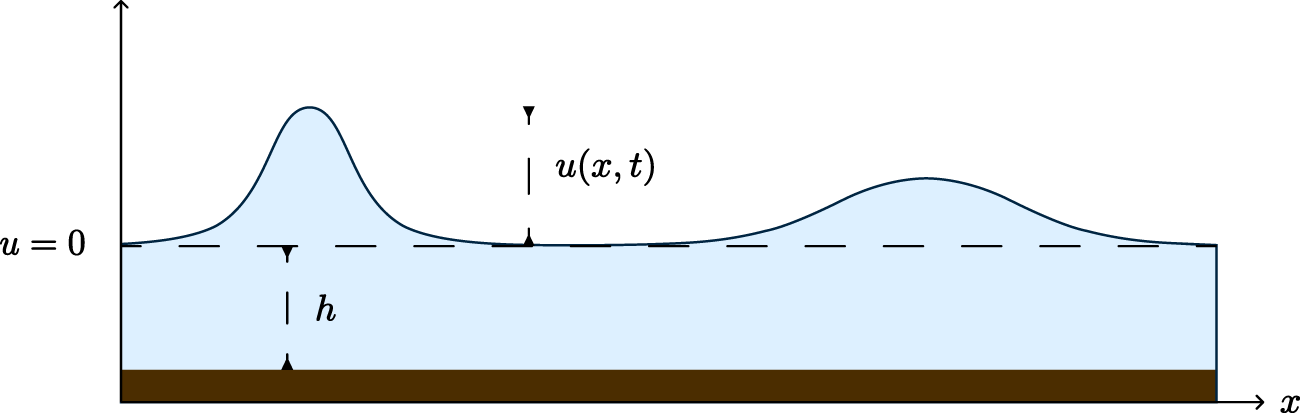


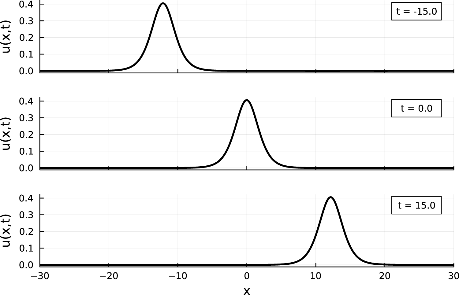
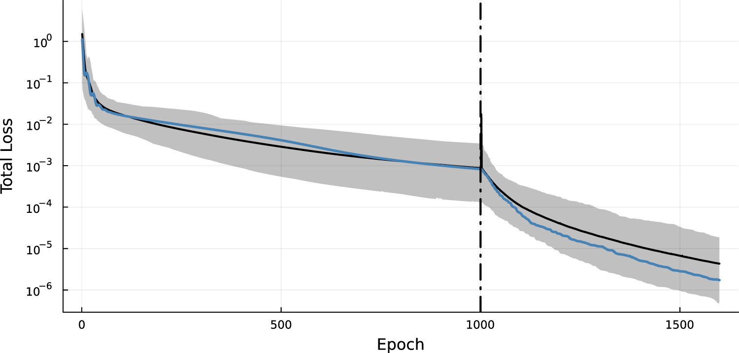

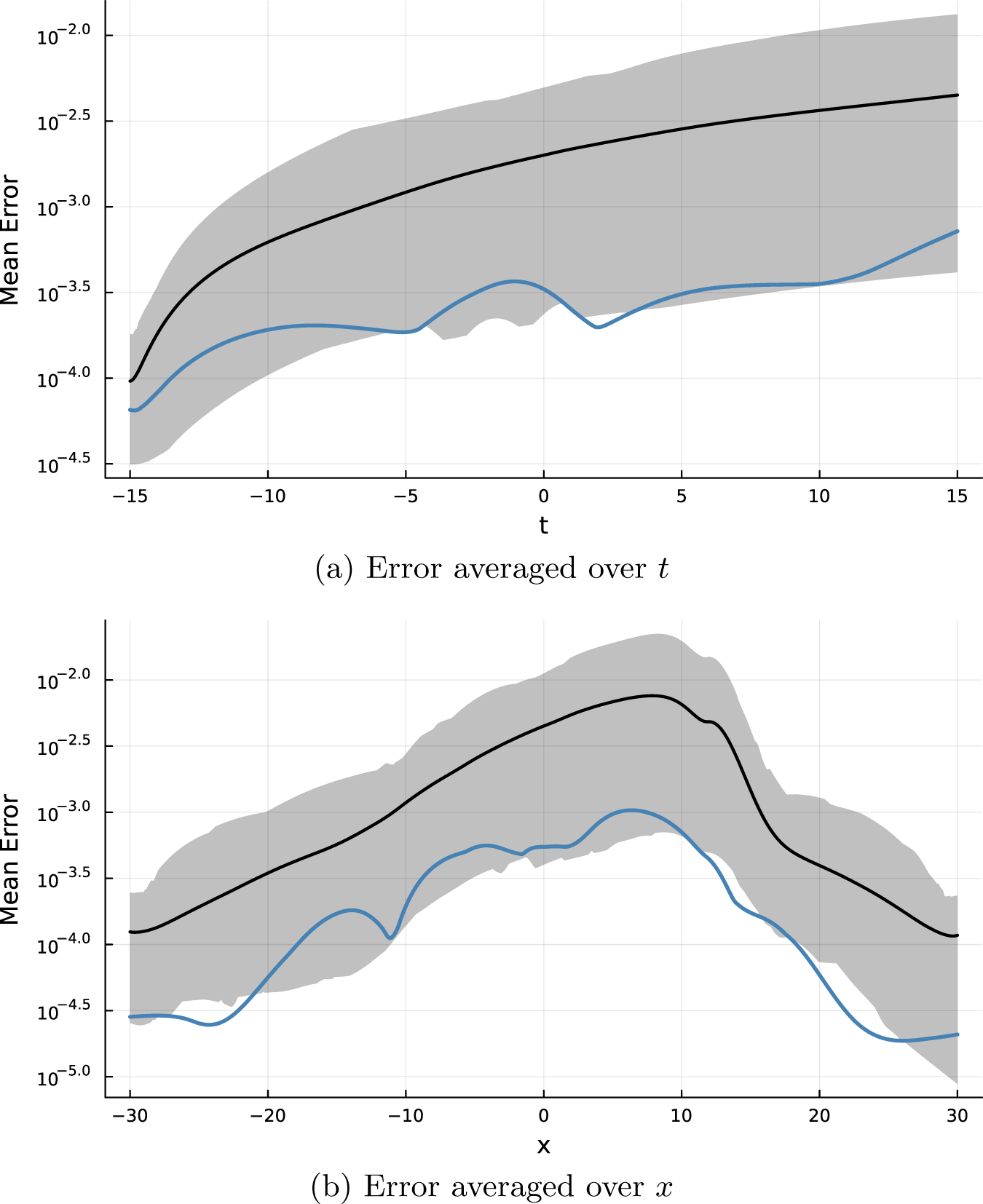


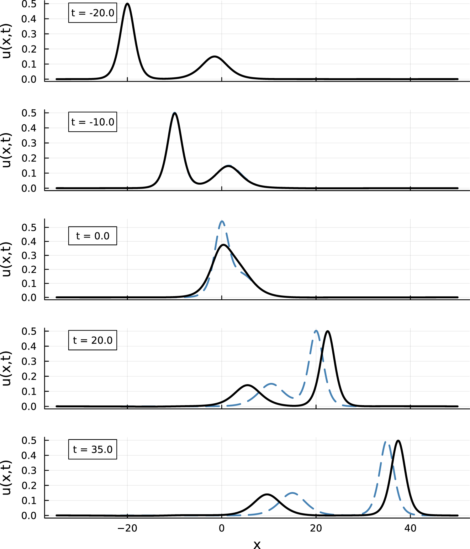
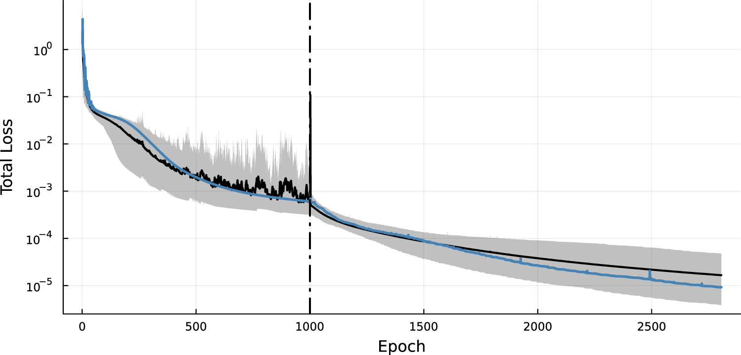
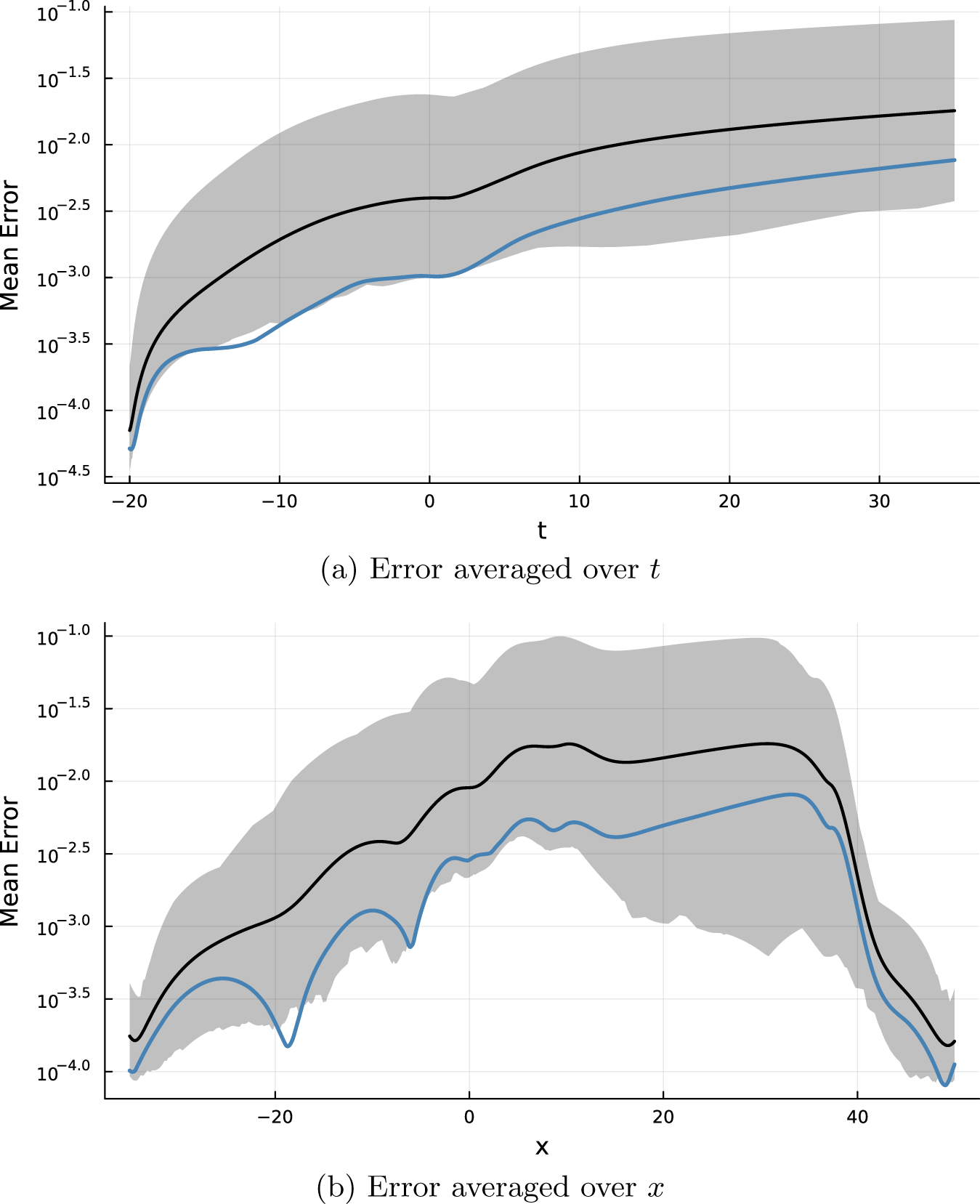


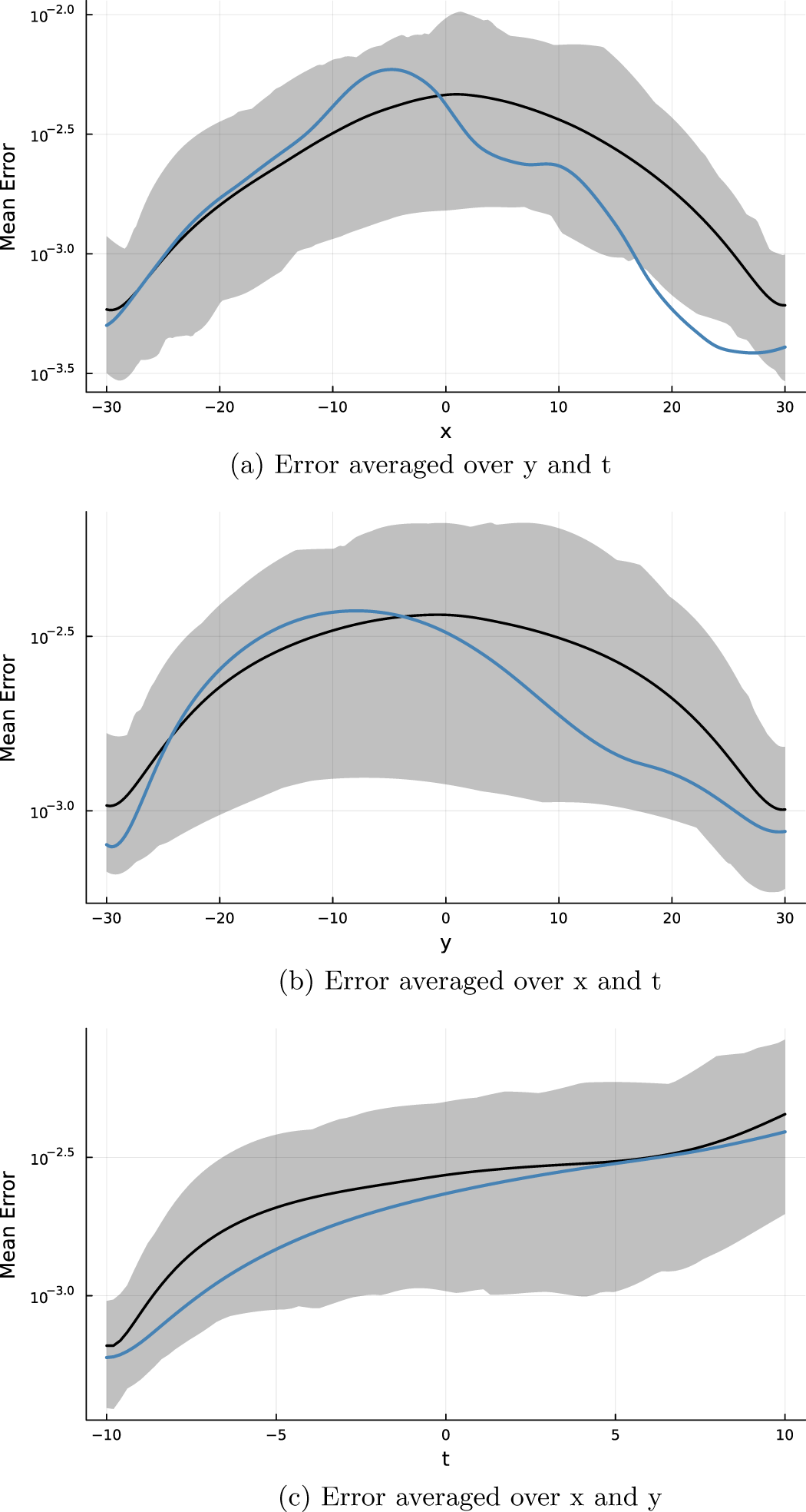


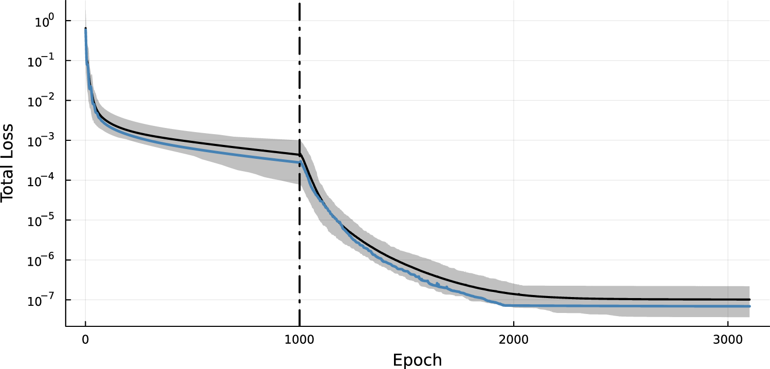

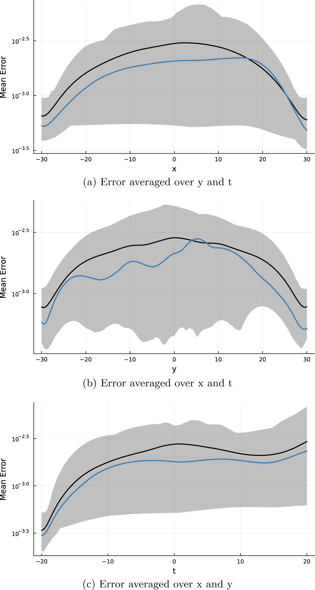


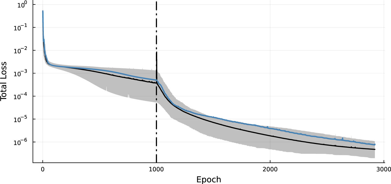

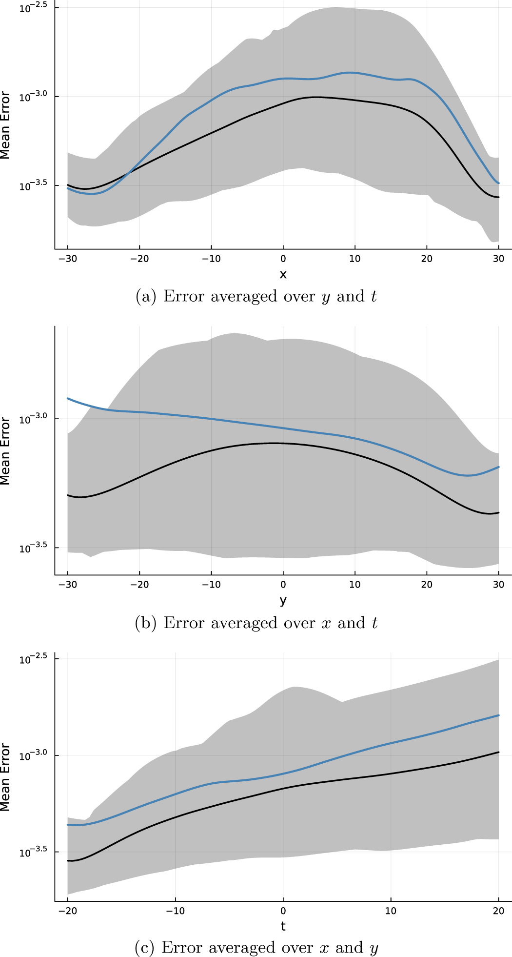


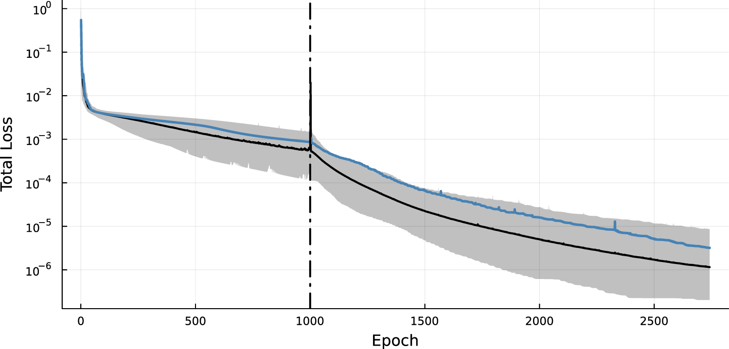


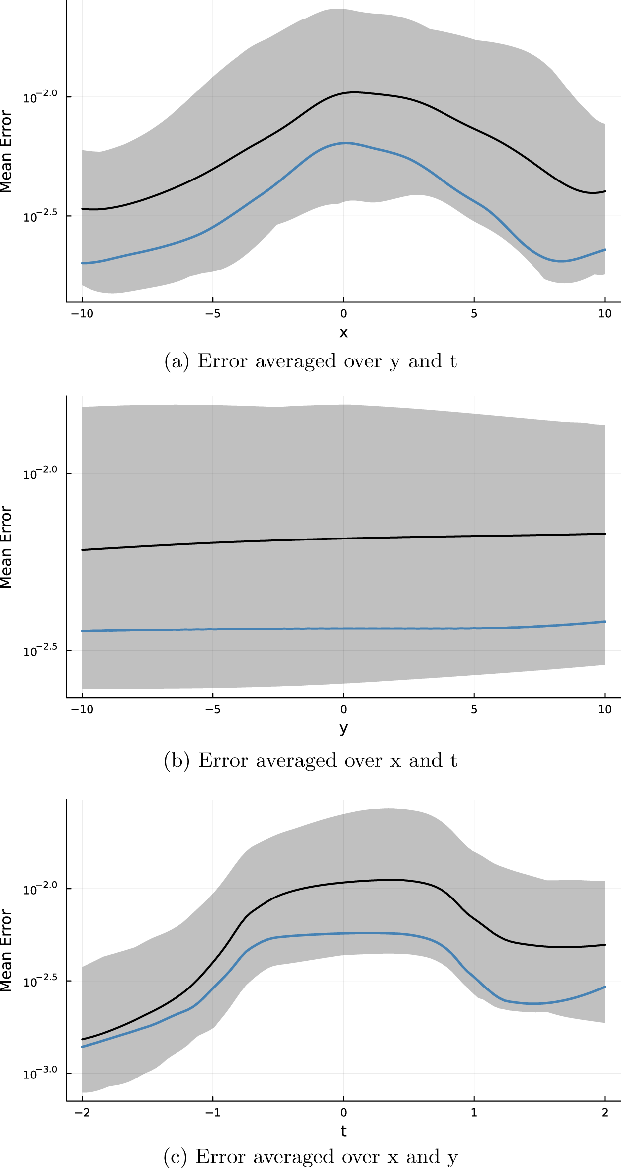
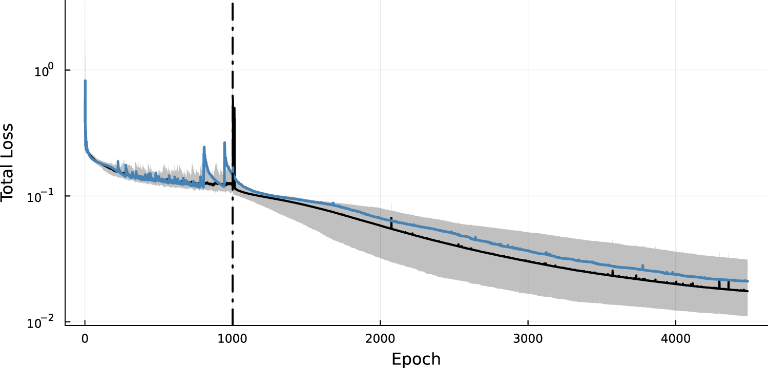
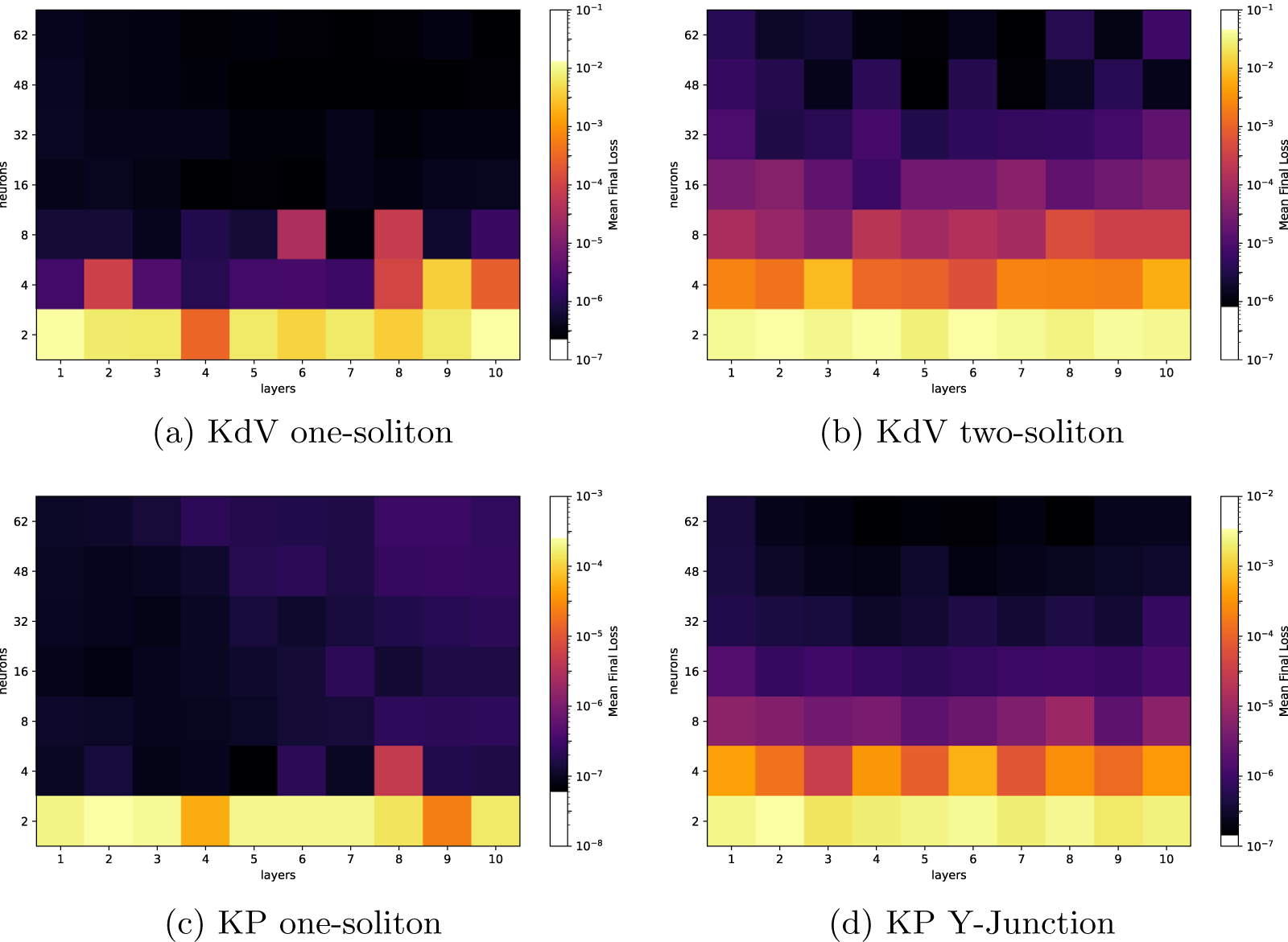

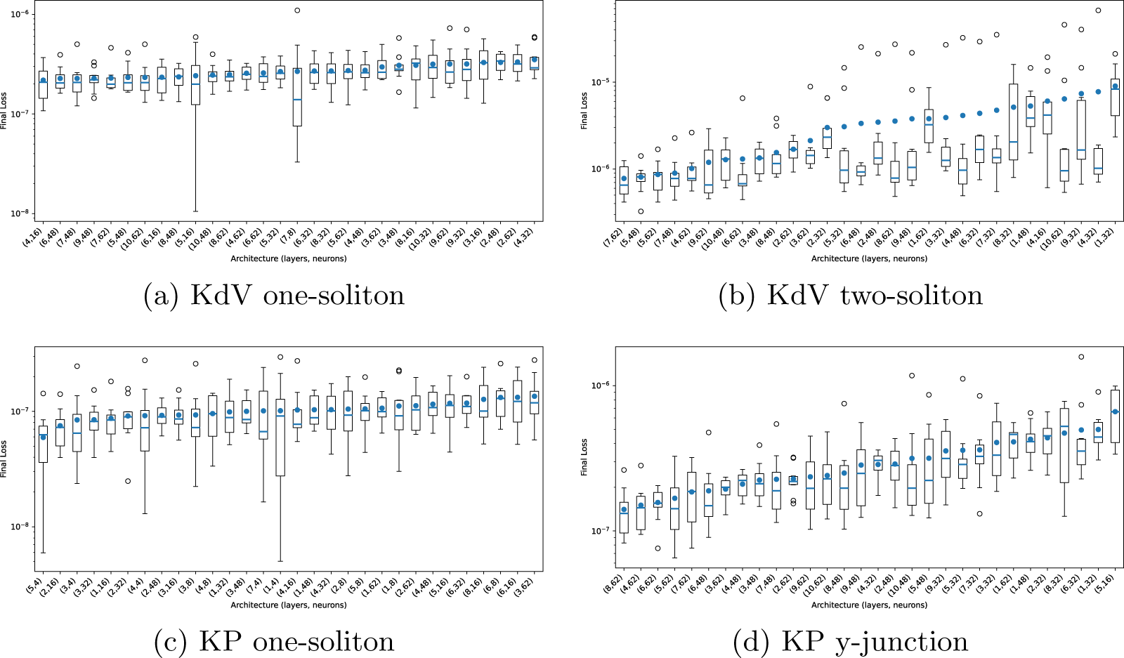


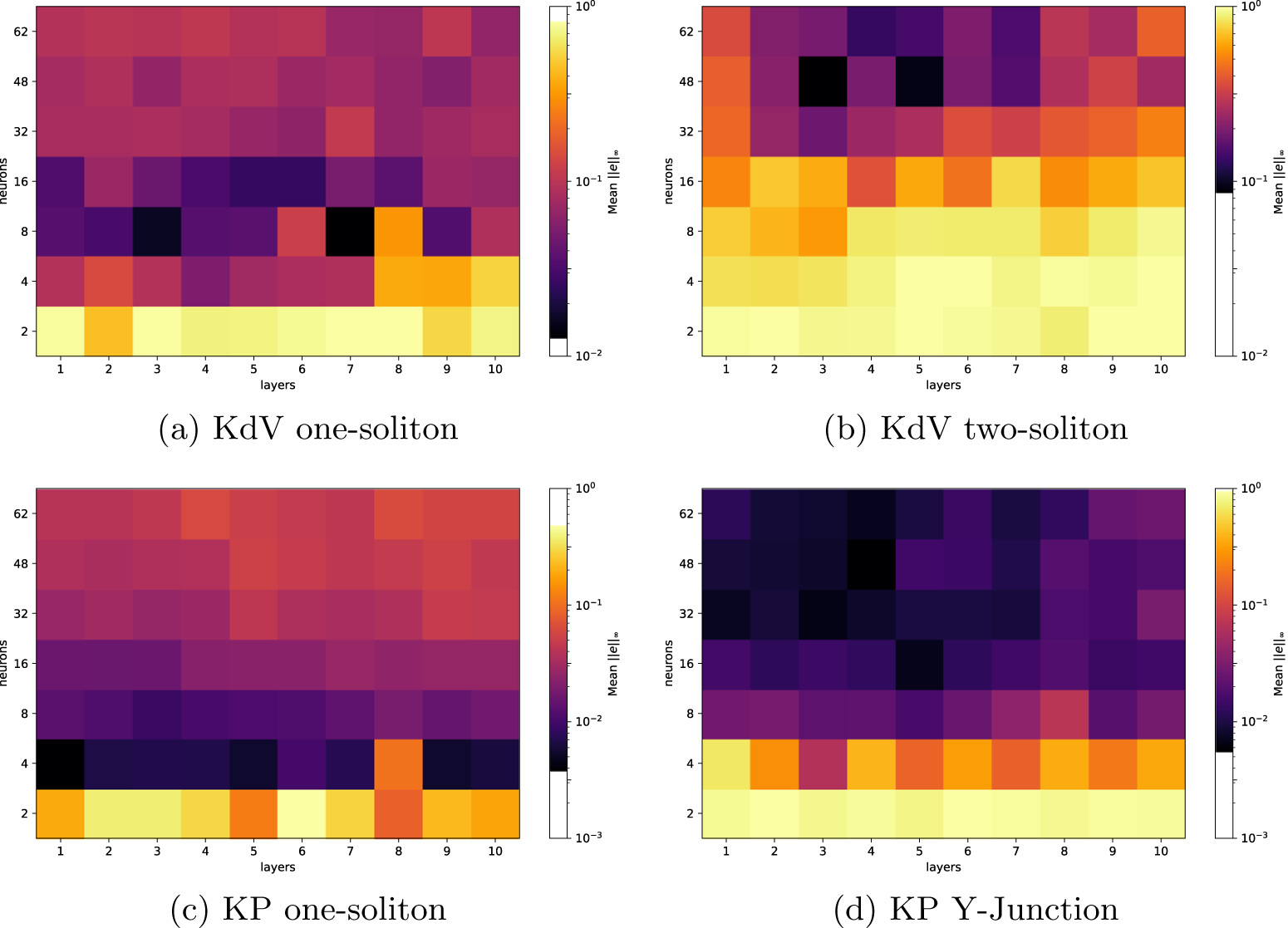


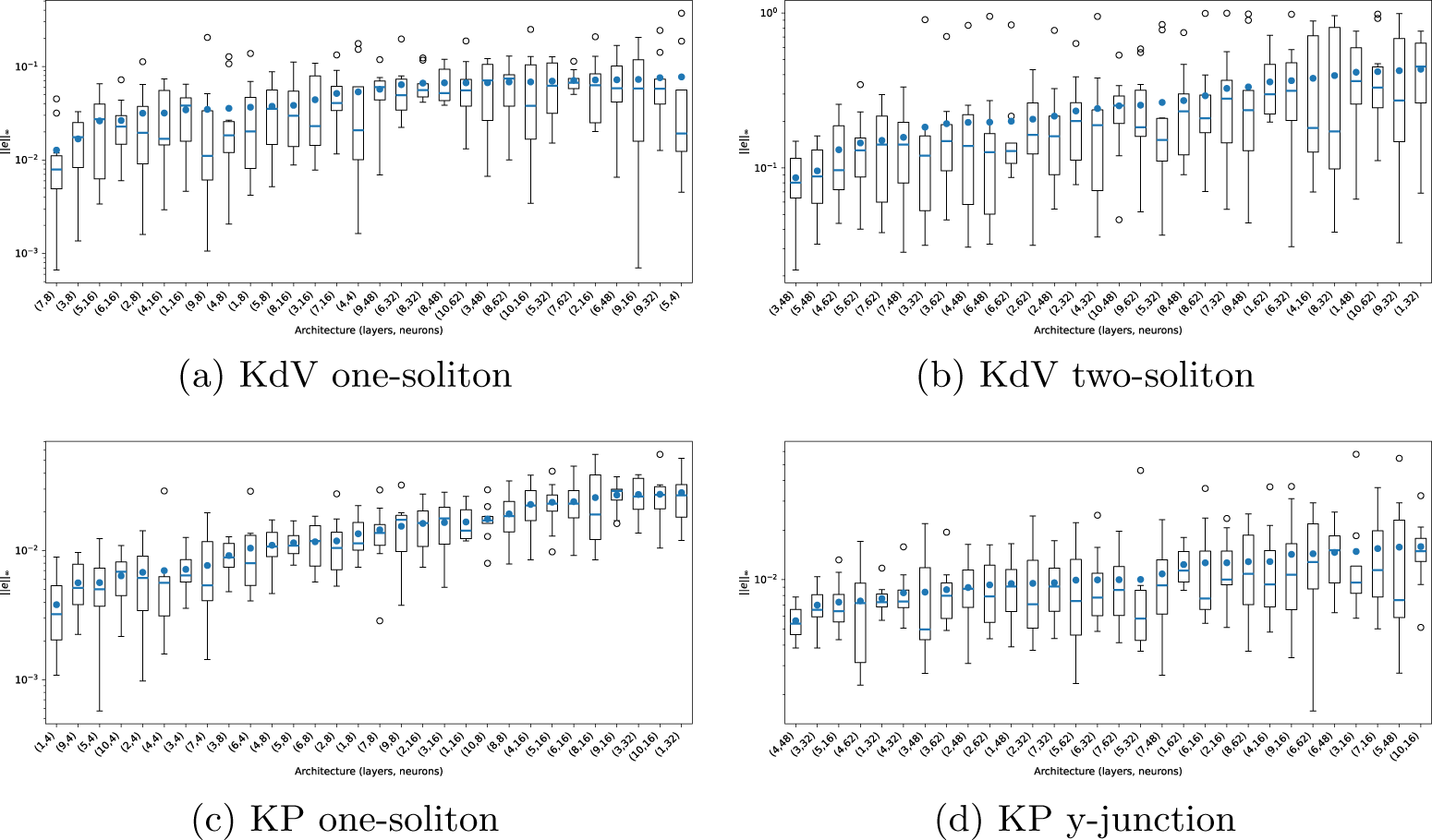


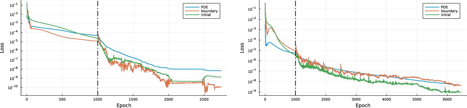
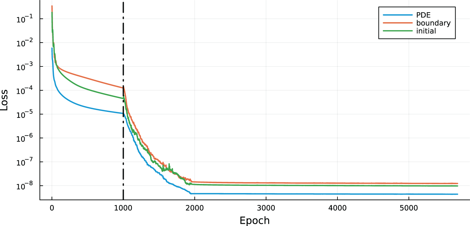
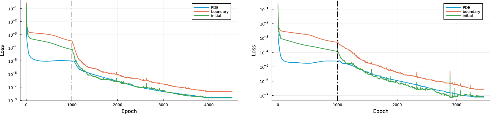
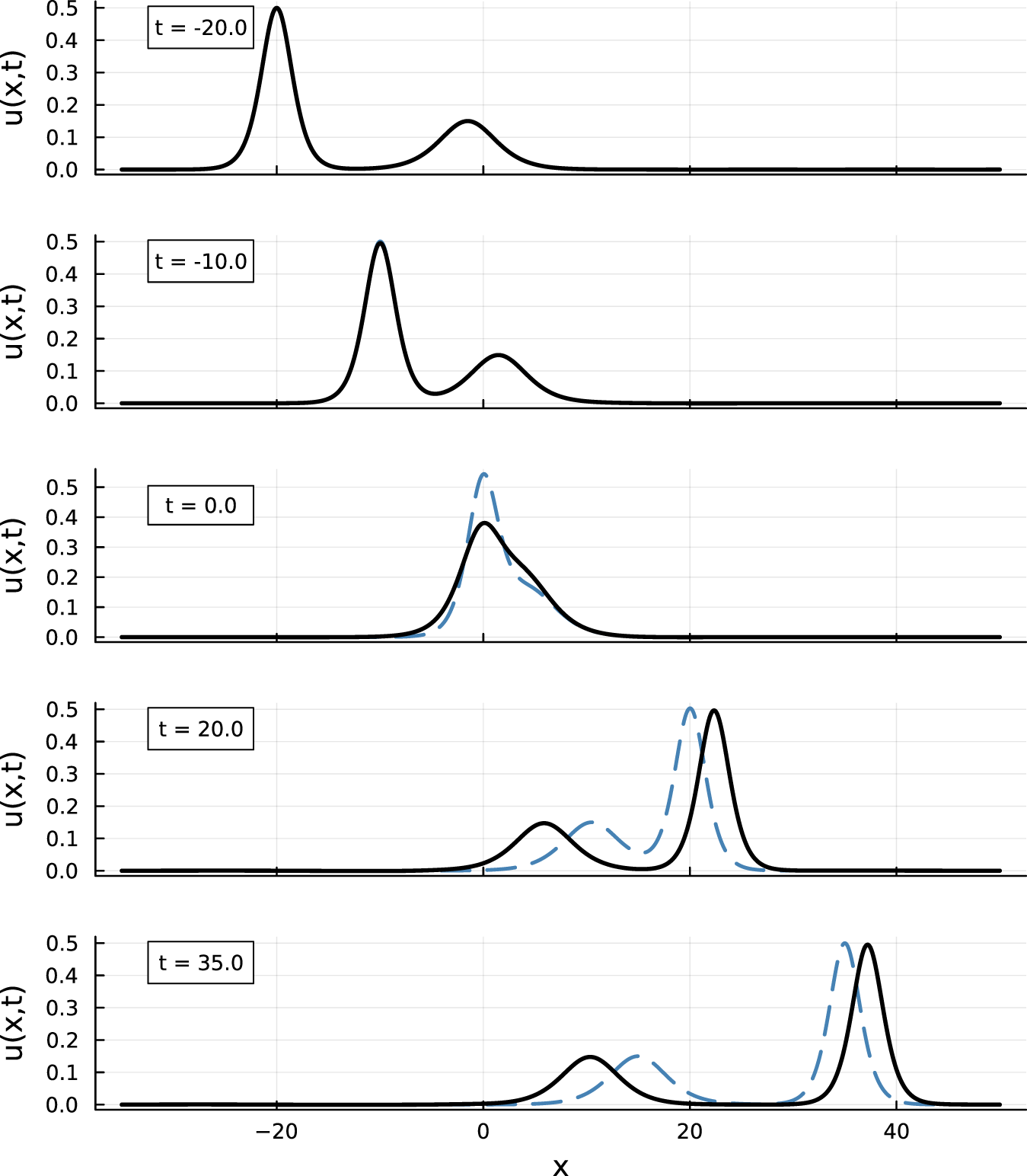
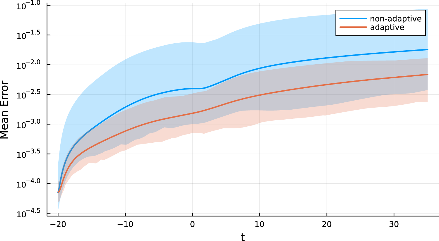


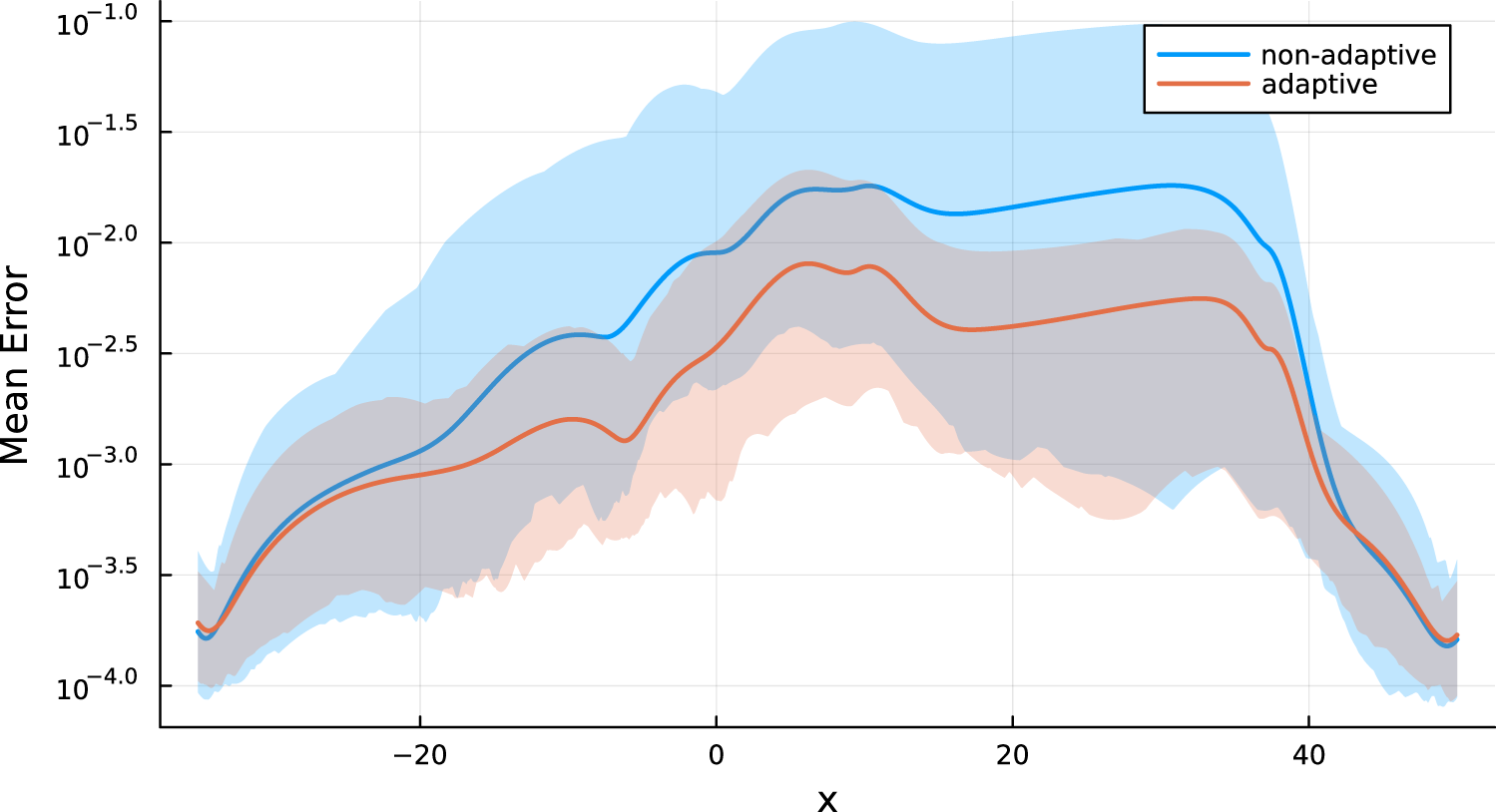


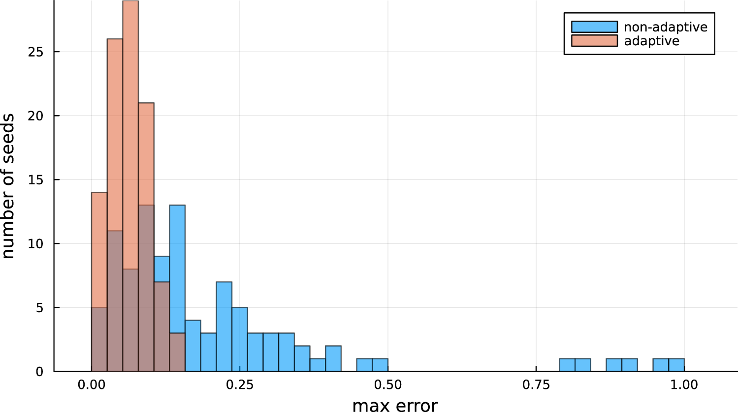

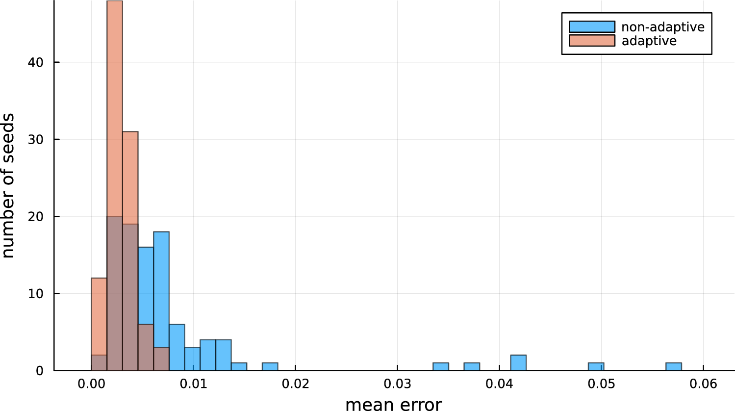
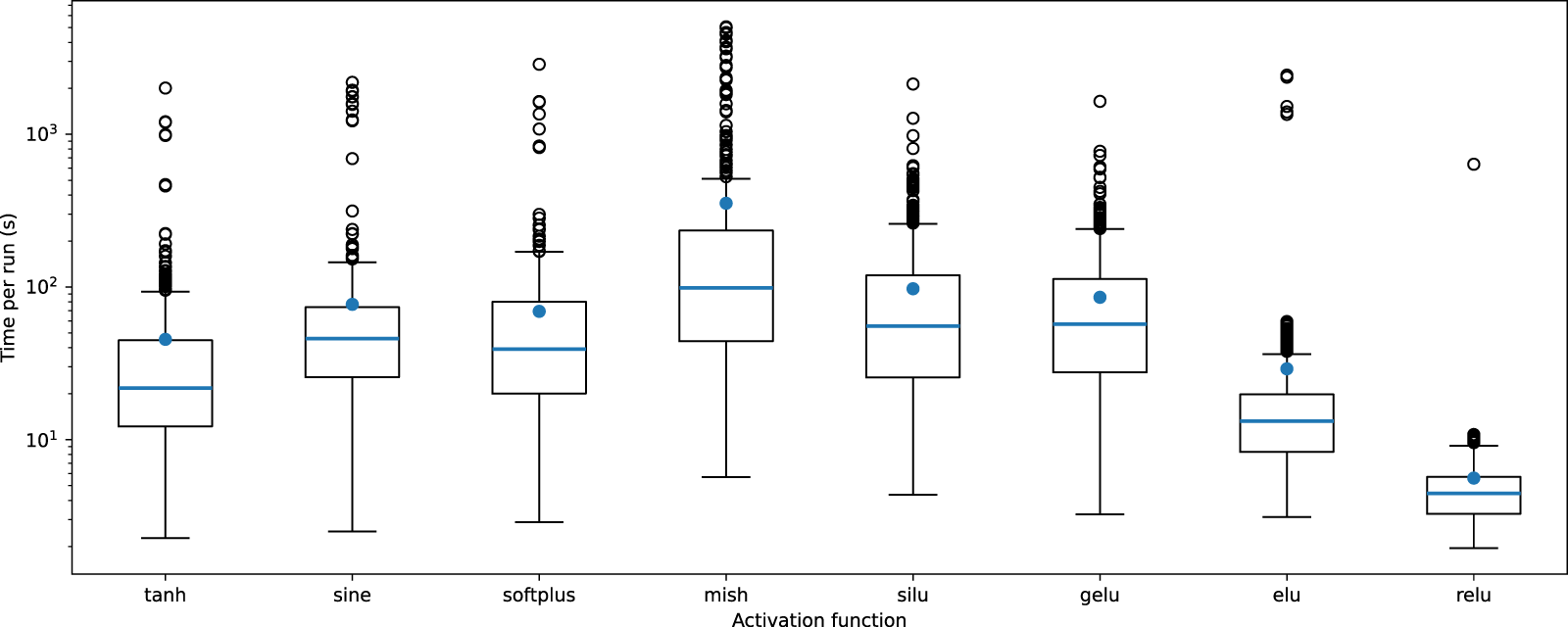


 Open access

