1. Introduction
Actuaries and financial risk managers use an economic scenario generator (ESG) to identify, manage and mitigate risks over a range of time horizons. In particular, pension schemes and other long-term businesses require ESGs to simulate projections of assets and liabilities in order to devise adequate risk mitigation mechanisms. ESGs thus need to provide reasonable simulations of the joint distribution of several variables that are required for the valuation of assets and liabilities. In this paper, we discuss how a graphical model approach is used to develop an ESG.
A wide range of ESGs are currently in use in the financial services industry. These models have varying levels of complexity and are often proprietary. They are periodically recalibrated and tend to incorporate a forecasting dimension. For instance, they may incorporate a vector autoregression (VAR) model. Additionally, many rely on a cascading structure, where the forecast of one or more variables is then used to generate values for other variables, and so on. In each case, these models face the difficult trade-off between accurately capturing short-term dynamics (requiring greater complexity) and long-term interdependencies. Further, the introduction of additional variables may require a significant reworking of the cascading structure in such models.
For the purpose of risk calculation over long periods, previous authors have adopted the simpler approach of modelling the underlying correlations between the innovations to the variables, for example, the residuals or the error terms in an autoregression. Graphical models achieve this in a parsimonious manner, making them useful for simulating data in larger dimensions. In graphical models, dependence between two variables is represented by an “edge” in a graph connecting the variables or “nodes”. This approach allows us to assume conditional independence between two variables (that are not directly connected by an edge) and to set their partial correlations to zero. The two variables could then be connected via one or more intermediate variables, so that they could still be weakly correlated.
An objective of this paper is to encourage the use of graphical models and demonstrate their appeal for actuarial applications. As a result, we compare different algorithms to select a graphical model, based on the Akaike information criterion (AIC), the Bayesian information criterion (BIC), p-values and deviance. We find them to yield reasonable results and relatively stable structures in our example. The graphical approach is fairly easy to implement, is flexible and transparent when incorporating new variables, and thus easier to apply across different datasets (e.g. countries). Similar to other reduced form approaches, it may require some constraints to avoid violation of both theory-based and practical rules. It is also easy to use this model to introduce arbitrary economic shocks.
We provide an application of the graphical model approach in which we identify an ESG suitable for use by a life insurance company or a pension fund in the United Kingdom that invests in equities and bonds. While more complex modelling of the short-term dynamics of processes is certainly feasible, our focus is on the joint distribution of innovations over the long-term. To this end, we seek the simplest time series dynamic that produces an adequate model, by fitting an autoregressive process to each of the series in our model and then estimate the graphical structure of the contemporaneous residuals. We find that simulations from this simple structure provide plausible distributions that are comparable to an established benchmark. The goal in our paper is to retain as simple a time series model as possible to highlight the potential of the graphical structure, even when there is a limited series of data available (as in some countries). However, we also discuss how graphical models can be used to model more complex dynamics if needed, such as to introduce nonlinear dependence through regime shifts.
Overall, we argue that this approach to developing ESGs is a useful tool for actuaries and financial risk managers concerned about long-term asset-liability modelling. Below, we provide a brief background on ESGs proposed for the insurance industry. In the next section, we provide a short introduction to the graphical modelling method we will apply. In sections that follow, we will first describe our dataset, and then using it as an illustration, discuss the various approaches to selecting an appropriate graphical model. We will also provide some comparisons to a published model.
1.1 Background and motivation
ESGs have been in use for a long time, and play a central role in quantifying the risks to the economic survival of a firm over the life of its commitments. Some of the key variables required to estimate the distribution of future assets and liabilities include returns to stocks and bonds, as well as discount rates.
A key requirement for an ESG is to present coherent future scenarios of all relevant variables jointly, rather than to simulate them without paying attention to their interlinkages. For a review of the considerations in developing and using an ESG, see Pedersen et al. (Reference Pedersen, Campbell, Christiansen, Cox, Finn, Griffin, Hooker, Lightwood, Sonlin and Suchar2016).
One of the earliest published models taking this into account, and aimed at actuarial requirements was that of Wilkie (Reference Wilkie1986). This model is based on a carefully calibrated cascading structure that builds up future scenarios in an explicit sequence, taking into account the dynamic properties of the individual variables being modelled. It has subsequently been updated and extended in a series of papers (Wilkie, Reference Wilkie1995; Wilkie et al., Reference Wilkie, ¸Sahin, Cairns and Kleinow2011). While the general principles remain the same, the authors have applied new techniques and have updated information about the original and newly introduced variables to generate fresh forecasts. In particular, Wilkie & ¸Sahin (Reference Wilkie and ¸Sahin2016, Reference Wilkie and ¸Sahin2017a,b,c, Reference Wilkie and ¸Sahin2018, Reference Wilkie and ¸Sahin2019) thoroughly analyse the model structure and estimation, and incorporate new methods to refine the modelling of individual and joint dynamics of different series.
Several other models and variations have been developed, both in the public domain and in the proprietary commercial domain (see e.g. Mulvey et al., Reference Mulvey, Thorlacius, Ziemba and Mulvey1998, Reference Mulvey, Gould and Morgan2000; Ahlgrim et al., Reference Ahlgrim, Stephen and Richard2004). Footnote 1 Huber (Reference Huber1997) has provided a detailed analysis of the Wilkie model. Other models developed along the same principles include Yakoubov et al. (Reference Yakoubov, Teeger and Duval1999). Whitten & Thomas (Reference Whitten and Thomas1999) and Ahlgrim et al. (Reference Ahlgrim, Stephen and Richard2005) are among papers that propose the introduction of nonlinear elements, such as threshold effects or regime switching. Chan (Reference Chan2002) proposed a general VAR moving average structure to overcome some of the restrictions in previous models. This is only a partial list of a large literature on ESGs based on a VAR representation. Other authors have proposed the inclusion of no-arbitrage constraints across markets when applying equilibrium models (see e.g. Smith, Reference Smith1996; Thomson & Gott, Reference Thomson and Gott2009).
In a cascading structure, one could, for instance, begin by modelling either the short or long government bond yield and the term spread. Together, these variables could act as inputs in the price inflation process. As an example, Mulvey et al. (Reference Mulvey, Thorlacius, Ziemba and Mulvey1998) model inflation as a diffusion process that depends on the short rate, the long rate and has a stochastic volatility component. These variables, along with inflation, then act as inputs to the next variable being modelled. At each stage, a number of constraints may be needed and the system then builds up into a tightly structured process with joint dynamics. In such models, there exists a natural tension between short-run dynamics and longer term predictability as in any VAR framework. Further, the procedure for constructing such structures often involves multiple testing schemes for model selection – an issue that may require more attention as the complexity of the individual models increases.
One of the motivations for the current paper is to offer a complementary approach to developing ESGs that is somewhat easier to implement and more flexible when one needs to incorporate new information. Graphical models provide a simple visual summary of the linkages being modelled and allow the modeller to use their judgement in a transparent manner when attempting dimension reduction. The models can generally be estimated and used to generate simulations easily and quickly.
As demonstrated by Ang & Piazzesi (Reference Ang and Piazzesi2003), one can improve the representation of the dynamics of variables such as interest rates by incorporating other correlated variables in the model, which is what the graphical model achieves without specifying more complex processes. Given that our goal is to capture more long-term stable relationships and allow for variation across them, the simplicity helps us avoid the trade-offs imposed by short-term versus long-term forecasting (see e.g. Christoffersen & Diebold, Reference Christoffersen and Diebold2000).
An early application of graphical models to risk estimation was proposed by Porteous (Reference Porteous1995). Subsequently, this model has been updated and applied in a number of papers (see e.g. Porteous & Tapadar, Reference Porteous and Tapadar2005, Reference Porteous and Tapadar2008a,b; Porteous et al., Reference Porteous, Tapadar and Yang2012; Yang & Tapadar, Reference Yang and Tapadar2015). As the primary focus of these papers was risk quantification of financial services firms, detailed discussions of the development and methodology of the ESG were not included. In this paper, we demonstrate the steps in building a graphical model for simulating economic scenarios and discuss the issues that arise.
2. Graphical Models
A graph,
 $$[{\cal G} = ({\cal V},{\cal E})]$$
, is a structure consisting of a finite set
 $$[{\cal V}]$$
of variables (or vertices or nodes) and a finite set of edges
 $$[{\cal E}]$$
between these variables. The existence of an edge between two variables represents a connection or some form of dependence. The absence of this connection represents conditional independence.
For instance, if we have a set of three variables
 $$[{\cal V} = \{ A,B,C\} ]$$
, where A is connected to B and not to C, but B is connected to C, A is connected to C via B. A is then conditionally independent of C, given B. Such a structure can be graphically represented by drawing circles or solid dots representing variables and lines between them representing edges. The graphical model described above with three variables, A, B and C, is shown in Figure 1. We can see that there is a path between A and C, which goes through B. The graphs we consider here are called undirected graphs because the edges do not have a direction (which would otherwise be represented by an arrow). Such graphs model association rather than causation.
A graphical model with three variables and two edges.

Another way of looking at graphical models is that they are excellent tools for modelling complex systems of many variables by building them using smaller parts. In fact, graphical models may be used to represent a wide variety of statistical models including many of the more sophisticated time series models used in actuarial science today. Recent standard and accessible texts on graphical models include Edwards (Reference Edwards2012) and Højsgaard et al. (Reference Højsgaard, Edwards and Lauritzen2012). The latter provides detailed guidance on the use of packages written in R to estimate graphical models. In this paper, we make use of these standard packages wherever possible. Our aim is to demonstrate the use of the undirected graph to develop a parsimonious representation of the economic variables that can then be easily used for simulation. Footnote 2
Graphical models are non-parametric by nature, but they may be used to represent parametric settings, a feature that is desirable for applications such as ours. Due to the easy translatability between the traditional modelling structure (covariance matrices) and the graphical structure in multivariate normal settings, we will focus on the parametric approach here and show that it leads to reasonable outcomes with our modelling strategy. Such models are known as Gaussian Graphical Models.
One of our key goals is to be able to represent the covariance structure with dimension reduction, and the graphical model will allow us to achieve that by effectively capturing conditional independence between pairs of variables and shrinking the relevant bivariate links to zero while allowing for weak correlations to exist in the simulated data. For the multivariate normal distribution, if the concentration matrix (or inverse covariance matrix) K = Σ−1 can be expressed as a block diagonal matrix, that is:
 $${\bf{K}} = \left[ {\begin{array}{*{20}c}{{\bf{K}}_{\bf{1}} } & {\bf{0}} & \cdots & {\bf{0}} \\{\bf{0}} & {{\bf{K}}_{\bf{2}} } & \cdots & {\bf{0}} \\\vdots & \vdots & \ddots & \vdots \\{\bf{0}} & {\bf{0}} & \cdots & {{\bf{K}}_{\bf{m}} } \\ \end{array}} \right]$$
then the variables u and v are said to be conditionally independent (given the other variables) if k uv = 0 where K = (k uv ). To achieve this block diagonal structure, variables may need to be reordered.
As the concentration matrix K depends on the scales of the underlying variables, it is sometimes easier to analyse the partial correlation matrix ρ = (ρ uv ), where:
 $$\rho _{uv} = \frac{{k_{uv} }}{{\sqrt {k_{uu} {\kern 1pt} k_{vv} } }}.$$
Note that ρ uv = 0 if and only if k uv = 0.
For our example graphical model in Figure 1, the partial correlation matrix would look like:
 $$\rho = \left[ {\begin{array}{*{20}c}1 & {\rho _{AB} } & 0 \\{\rho _{AB} } & 1 & {\rho _{BC} } \\0 & {\rho _{BC} } & 1 \\\end{array}} \right],$$
where ρ AB = 0 and ρ BC = 0. So, variables A and C are independent given variable B. Note that this could still generate non-zero unconditional correlation between A and C.
Before illustrating the application of this structure, we will first describe the data in the next section.
3. Data
In order to build a minimal economic model, which can be used by a life insurance company or a pension fund in the United Kingdom, we require retail price inflation (I), salary inflation (J), stock returns and bond returns over various horizons.
The data we use in this paper have been generously provided by David Wilkie, who has carried out a range of checks and matching exercises to construct all the relevant time series. Following his procedure in Wilkie (Reference Wilkie1986), we model dividend yield (Y), dividend growth (K) and Consols yield (C) to construct stock and bond returns. Consols yield is the yield on perpetual UK government bonds.
We use the complete dataset provided by David Wilkie, which consists of annual values from 1926 to 2017 as at the end of June each year. An excerpt of the data can be found in Wilkie et al. (Reference Wilkie, ¸Sahin, Cairns and Kleinow2011).
4. Modelling
We are interested in simulating the selected variables jointly, so we may first wish to take a look at the historical pairwise correlations. These are given in Table 1. It appears that price and salary inflation and long-term bond yields are all highly correlated with each other, but the other correlations are relatively smaller. A graphical model promises to provide the flexible framework needed to generate scenarios consistent with this long-run dependence structure.
Historical correlations

4.1 Correlations in levels or in innovations
As discussed above, graphical models may capture VAR frameworks and models with latent variables or states, but our aim is to provide an adequate model that is as simple as possible. When simulating, there is a philosophical question as to whether one should produce scenarios from a tightly structured model of the levels of the variables, or whether one should focus on the innovations in the time series processes of these variables. By construction, the innovations should be i.i.d once a well-specified regression model has been fitted. We take the view that contemporaneous changes in variables beyond those predicted by their own past values offer a useful handle on the range of scenarios to be produced (see e.g. Jondeau & Rockinger, Reference Jondeau and Rockinger2006, for the usefulness of such an approach).
Over the 90-year history of these variables, there have been several events, but one could still argue that there is long-term mean reversion in most series, albeit at different rates. This may be a good reason to focus our attention on modelling the joint innovations in the series. Rather than model the joint dynamics of variables using a large number of constraints and parameters, we can minimise the number of constraints required by restricting them to situations that would rule out inadmissible values.
Given that the aim of our ESG is to emphasise long-run stable relationships and to generate a distribution of joint scenarios, we take the approach of estimating the joint distribution of the residuals of individual time series regressions. This focuses on the dependence between innovations and, we argue, may allow for a richer set of scenarios generated with relatively simple models. For each variable, we will first estimate a time series model independently and then we will fit a graphical model for the time series residuals across variables.
At the annual frequency we consider here, the dynamics of the variables can arguably be adequately represented by a simple AR(1) process in most cases. For each time series X t , we use the following AR(1) time-series model formulation:
 $$\mu _x = E[X_t ]$$
 $$Z_t = X_t - \mu _x $$
 $$Z_t = \beta _x {\kern 1pt} Z_{t - 1} + e_{x,t} \quad {\rm{where}} \quad e_{x,t} \sim N(0,\sigma _x^2 ).$$
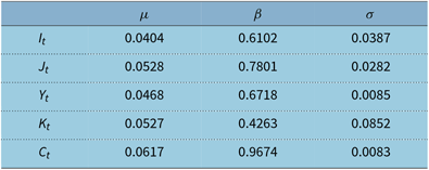
The parameter estimates from the AR(1) regressions are provided in Table 2.
Time series parameter estimates

Note: All parameter estimates for μ and β are statistically significant at the 5% level.
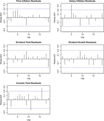
In addition, the fit appears satisfactory in the sense that there does not appear to be significant residual dependence in the errors. Partial autocorrelation plots of the residuals from these regressions are provided in Figure 2 for reference. While an AR(1) fit appears adequate for the purposes of our model, one can choose an alternative univariate time series model if deemed appropriate, as we are interested in the innovations from the model.
Plots of partial autocorrelation functions (PACF) of the residuals.

4.2 Fitting a graphical model to the residuals
To estimate a Gaussian Graphical Model for the residuals, we assume that:
 $${\bf{e}}_{\bf{t}} = (e_{I_t } ,e_{J_t } ,e_{Y_t } ,e_{K_t } ,e_{C_t } ) \sim {\cal N}({\bf{0}},\Sigma ).$$
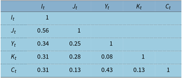
Estimation is carried out based on maximum likelihood, with model selection explained in detail in the next subsection. Footnote 3 The correlations between the residuals are given in Table 3.
Correlations of residuals

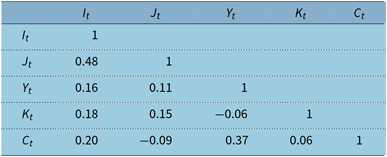
The resulting partial correlation matrix is given in Table 4. Clearly, some of the partial correlations in the matrix are small. Our goal is to identify the graph(s), with the minimum number of edges, which describe the underlying data adequately.
Partial correlations of residuals

As there are five variables in the model, the minimum number of edges required for a connected graph (i.e. where there exists a path between any two nodes) is 4. The graph with the maximum possible number of edges is the saturated model with 5 C 2 = 10 edges. We will call this Model ES (E for edges and S for saturated). The model with no edges is the independence model, that is, all variables are independent of each other, and we will call it Model E0 (as there are no edges).
In total, there are 210 = 1024 distinct models possible. But we will focus only on those models that are selected, based on certain desirable features.
4.3 Desirable features and model choice
Selection of a graphical model can be carried out by traditional statistical criteria. This is usually done in an iterative procedure, where we consider our model selection criterion of choice before and after adding (or removing) an edge between two variables. One may begin with Model E0 or ES and proceed in a pre-defined sequence. In each case, disciplined judgement may be applied, for instance, by plotting the p-values associated with individual edges and choosing a desired cut-off point. The statistical criteria include AIC, BIC, p-values of individual partial correlation estimates and deviance. Footnote 4 Below, we provide a set of tables summarising the results of the estimation procedures, followed by a discussion of the criteria used in the procedures.
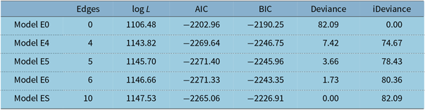
In Table 5, we present summary statistics of the following models:
Summary of graphical model fit

Model E0: The independence model with no edges.
Model E4: The optimal model according to BIC.
Model E5: The optimal model according to AIC.
Model E6: The optimal model using simultaneous p-values at confidence level α = 0.6.
Model ES: The saturated model with all possible edges.
The graphical structure of Models E4, E5 and E6 are given in Figure 3.
Optimal graphical models based on different selection criteria.

Parameter estimation based on the maximum-likelihood approach aims to maximise the likelihood, or log-likelihood log L, of a specified model. Let l̂ be the maximised value of the log-likelihood. Usually, a model with a higher maximised log-likelihood is preferred.
In a nested model framework, a model with more parameters will naturally lead to a higher log-likelihood. This is evident from the log L measures given in Table 5, where the saturated Model ES has the highest log-likelihood and the independence Model E0 has the lowest log-likelihood. But, if parsimony is a desirable feature, a saturated model need not be the preferred model.
In a nested model framework, one can define the notion of Deviance of a model, with maximised log-likelihood l̂, as
 $${\rm{Deviance}} = 2(l_{{\rm{s}}at} - l),$$
where l̂ sat is the maximised log-likelihood of the saturated model. So Deviance represents the log-likelihood ratio relative to the saturated model. On the other hand, iDeviance of a model, with maximised log-likelihood l̂, measures the log-likelihood ratio relative to the independence model and is defined as
 $${\rm{iDeviance}} = 2(l - l_{{\rm{i}}nd} ),$$
We can see from the Deviance and iDeviance values in Table 5 that Models E4, E5 and E6 are much closer to the saturated model than the independence model.
Among these nested models, one can define optimality based on penalised log-likelihood, where a penalty term is introduced to reflect the number of parameters in the model. Typically, this requires minimising the negative of a penalised likelihood:
 $$- 2 \log L + k \times p,$$
where p is the number of (independent) parameters and k is an appropriate penalty factor.
Different values of k are used in practice, for example, k = 2 gives the AIC and k = log n, where n is the number of observations, gives the BIC.
In Table 5, Model E4 is the optimal model according to BIC and Model E5 is the optimal model according to AIC.
Model E6 is obtained using a special form of thresholding called the SINful approach due to Drton & Perlman (Reference Drton and Perlman2007, Reference Drton and Perlman2008). The principle here is based on a set of hypotheses:
 $${\cal H} = \{ H_{uv} {\kern 1pt} :{\kern 1pt} e_u {\kern 1pt} {\kern 1pt} \bot \bot e_v {\kern 1pt} |{\kern 1pt} allothervariables\} ,$$
for which the corresponding nominal p-values are
 $${\cal P} = \{ p_{uv} \}$$
. These are then converted to a set of simultaneous p-values
 $$\tilde {\cal P} = \{ \tilde p_{uv} \} $$
, which implies that if H
uv
is rejected whenever p̃
uv
< α, the probability of rejecting one or more true hypotheses H uv is less than α.
In particular, Drton & Perlman (Reference Drton and Perlman2008) suggest two α thresholds to divide simultaneous p-values into three groups: a significant set S, an intermediate set I and a non-significant set N and hence the name SINful.
Figure 4 plots the simultaneous p-values for our dataset. The significant set, S, contains the edges between the residuals between price and salary inflation and also between dividend yield and Consols yield, even at a level of α = 0.01. Setting the second α threshold at 0.6 leads to the inclusion of 4 edges in the intermediate set I. These edges connect price inflation to all other variables and salary inflation to dividend growth. The remaining 4 edges form the non-significant set N. The resulting model using the edges in sets S and I produces Model E6 in Table 5 and Figure 3. Here, we have used judgement from a visual overview of the p-values to determine that there appear to be three distinct groups of edges. One could potentially choose 0.4 or 0.5 as the threshold in place of 0.6. However, this claim is equivalent to arguing that edges 1–3 and 2–4 belong to the set N, which one may or may not be comfortable claiming. Thus, this process remains transparent.
Plots of simultaneous p-values.

4.4 Other desirable features
Our next step will be to use the models above to generate scenarios over long periods in the future. For this purpose, in addition to dimension reduction, the modularity feature of the graphical model becomes very important.
A clique is a subset of variables in a graph such that all the variables in this subset are connected to each other. In other words, the subgraph represented by the clique is complete or saturated within itself. A maximal clique is one that is not the subset of another larger clique. When simulating variables using the multivariate normal distribution, such a clique is the unit from which we simulate. As a result, if the maximum size of a clique exceeds 3, then the gains from dimensionality reduction in estimation are significantly forfeited at the time of simulation. Graphs with such a preferred structure are referred to as triangulated. Visual evaluation of the graphical structure to address this is therefore a useful instance of applying judgement while choosing between models. In all the models, E4, E5 and E6, the structures are amenable to simulation due to the cliques being at most of size 3.
Another way to characterise this desirable property is through the graph’s decomposability, which allows for the derivation of an explicit MLE formula (see e.g. Edwards, Reference Edwards2012, and references therein). Essentially, decomposability implies the ability to describe the model in a sequential manner, such as in the form of a set of regressions. When simulating from an estimated model, this allows us to simulate variables in a sequence, conditional on the realisations of previous variables. The standard stepwise model selection algorithms usually allow the user to automatically disregard non-decomposable graphs.
Overall, of the three models we have identified, Model E4 is the minimal. However, the addition of the two links to get to Model E6 is intuitively appealing and consistent with economic theory as well as empirical evidence. It is well known that inflation expectations influence Consols yields (Campbell & Ammer, Reference Campbell and Ammer1993) and we also expect salary inflation and dividend growth to be related over the long term. Allowing for these links (albeit with weak correlation) helps in using our simple dynamic structure to capture these associations in the distribution of scenarios.
4.5 Scenario generation
Using Model E6 as an example, we outline the steps required for simulating future economic scenarios:
Step 1: The initial values of the economic variables, that is, (I 0, J 0, Y 0, K 0, C 0) are set at their respective observed values at the desired start date.
Step 2: To simulate (I t , J t , Y t , K t , C t ) at a future time t, given their values at time (t − 1), we first need to generate the innovations: e t = (e I t , e J t , e Y t , e K t , e C t ).
For Model E6, as can be seen from Figure 3, (e I t , e J t , e K t ) and (e I t , e Y t , e C t ) are the two cliques with e It being the common variable. We choose one of the cliques, say (e I t , e J t , e K t ), and simulate it from the underlying trivariate normal distribution. Then the other clique, (e I t , e Y t , e C t ), is simulated using a bivariate conditional normal distribution (e Y t , e C t ) given the value of e I t already simulated for the first clique. This shows how a graphical model approach can help reduce the computationally intensive task of simulating from a five-dimensional normal distribution to two simpler tasks of simulating from a trivariate and a bivariate normal distributions. In other words, for standard matrix inversion algorithms, it is a decrease in complexity from O(53) to O(33).
Using the simulated innovations (e I t , e J t , e Y t , e K t , e C t ), the values of (I t , J t , Y t , K t , C t ) can then be calculated using equations (4)–(6).
Step 3: Step 2 is repeated sequentially for the required time horizon to obtain a single realisation of a simulated future scenario.
Step 4: Steps 1–3 are then repeated for the desired number of simulations.
5. Simulation Results
We generate simulated values starting from the last data point available, which is 2017. In this example, we have produced 10,000 paths for the joint set of variables.
In addition to the scenarios generated through the graphical model, we also simulate the same number of paths based on the Wilkie model as a benchmark. In what follows, we will present the results alongside to allow for a discussion of the performance of our approach.
5.1 Marginal distributions
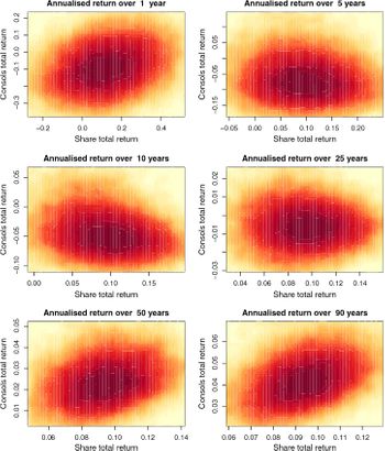
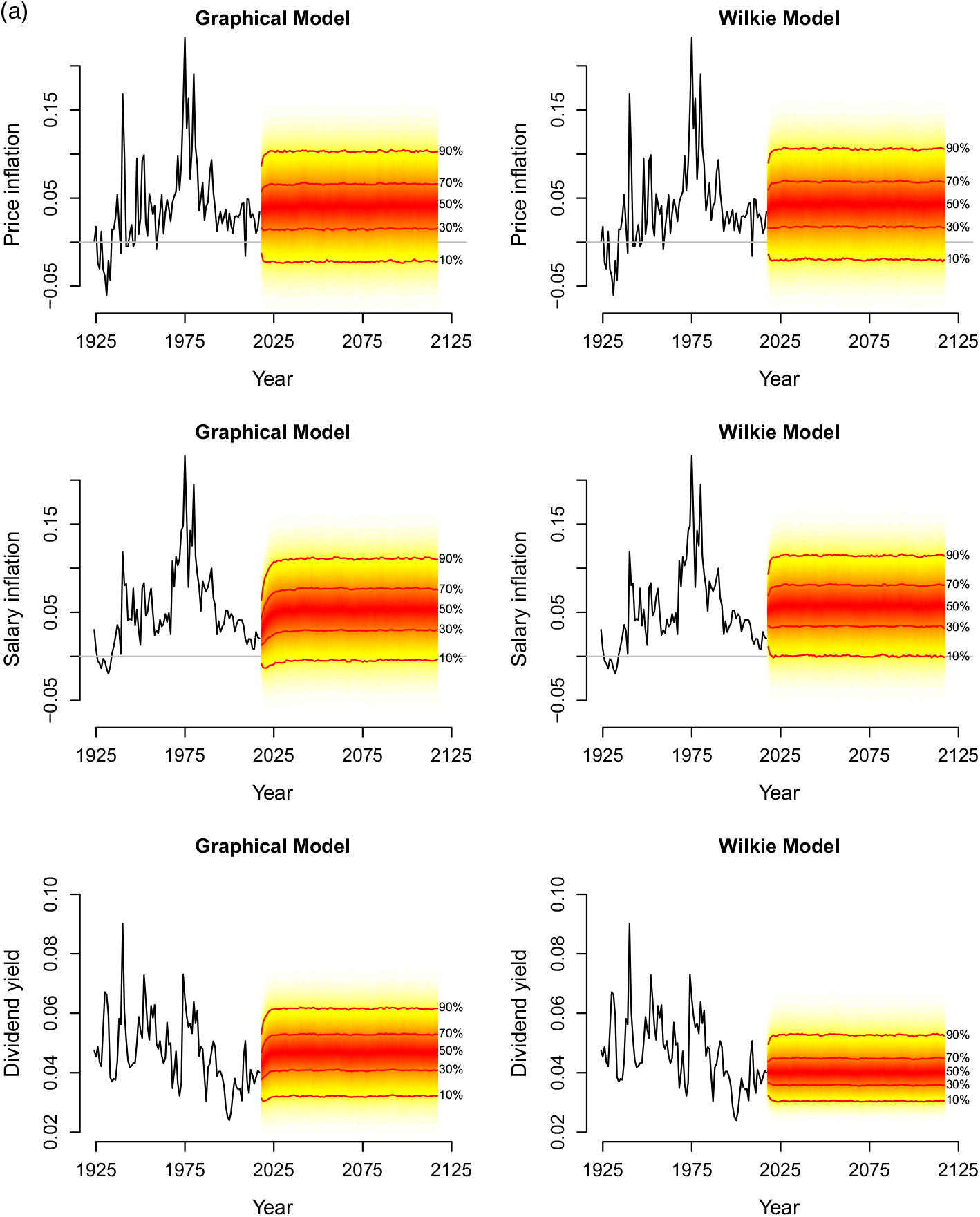
The simulation results can be viewed in terms of the marginal distributions of the variables and also in terms of their joint realisations. As a first sense check, we look at “fan charts” of the distributions of the five variables over the length of the simulations. These charts, based on Model E6 are presented in Figure 5. Models E4, E5 and E6 produce qualitatively similar results, so we show the plots for Model E6 as it has an intuitively appealing structure. For each variable, we place the chart from the Wilkie model alongside for easy visual comparison.
(a) Fanplots of simulations of price inflation, salary inflation and dividend yield from Model E6 and the Wilkie model.
(b). (continued). Fanplots of simulations of dividend growth and Consols yield from Model E6 and the Wilkie model.

The different speeds of convergence to the long-term mean are clearly visible across the different series. However, this is not simply an artefact of the different AR(1) estimates. While correlations in innovations feed into the cross-autocovariances of the series, the impact is varied on account of the different levels of memory in the processes. This is consistent with what we would expect over the short-term when starting the simulation from the current values of the series. In the long run all series have marginal distributions around their long-term means.
It also appears that the overall long-term picture of the marginals from our model are broadly similar to those from the Wilkie model. The main differences (albeit small) appear in the slower rate of mean reversion of the forecasts for salary inflation. The graphical model also generates a wider distribution of Consols and dividend yields than the Wilkie model.
The fan charts offer a useful sense-check as they can help identify potential violations of common sense economic constraints that one would like to avoid in the simulations. For instance, due to the exceptionally low long-term bond yields in the recent environment, we have imposed a constraint that the long-term yield does not fall below 0.05%. Should a value below this be predicted, it is simply set at the minimum value instead. While we have chosen this value to be consistent with current practice, recent experience suggests that the modeller may choose to lower the boundary or even do away with this constraint altogether. The model without the constraint does not preclude negative yields.
These types of constraints may have an impact on the correlations among the simulated variables, so it may also be useful to check the correlations, which we do next.
5.2 Distribution of correlations along simulated paths
We can also examine the range of “realised” or estimated correlations that arise in the simulated data. This helps get an additional view of the risk captured in the range of simulated scenarios, as estimated correlations would vary for each path or sample.
In Figure 6, we provide the pairwise correlations among the simulated versions of the variables based on Model E6 and the Wilkie model. For each simulation path we calculate one estimate of the correlation. We then plot the distribution of these correlation estimates across the simulations.
Correlations of variables for simulations from the Model E6 and the Wilkie model.
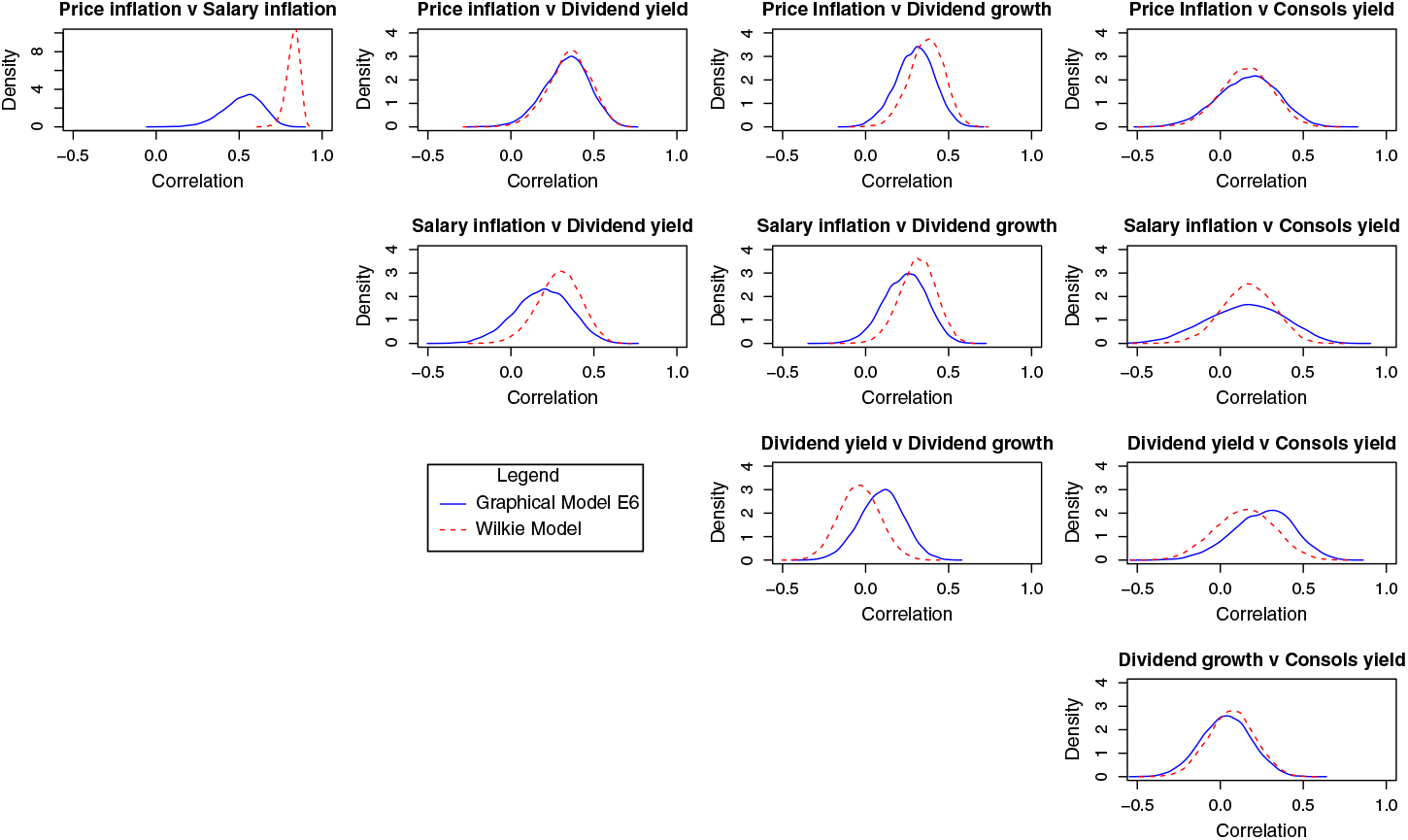
While many of the correlation profiles are very similar between the two approaches, there is a pronounced difference in the case of price and salary inflation. One might argue that the correlation in the Wilkie model is very constrained due to the model structure, it is also the case that the graphical model produces a very wide range of correlation values for the two variables. The differences in correlation profiles may partly be explained by the differences in persistence and variability between retail price inflation and salary inflation, and partly as a consequence of the Gaussian structure of the graphical model and its focus on innovations (as compared to the Wilkie model’s approach). However, it is not clear that one outcome is preferred to the other, so we do not consider any remedies.
5.3 Bivariate heat maps
The policy-oriented user is ultimately interested in the joint values of stock and bond returns indices, inflation and wages that the models generate. To discuss the output in this context, we plot the bivariate heat maps generated by the simulations for Model E6 and the Wilkie model. The pairs we consider are: first, annual stock returns and annual bond returns; and second, annual price inflation and annual salary inflation. We overlay the map with annual observations of the relevant pairs from the historical data available. These plots are provided in Figures 7 and 8, respectively. The heatmaps represent densities that integrate to 1, with the same colour representing the same quantile level. Only very subtle differences can be observed across the models, and they all do an arguably reasonable job of capturing the historical distribution. The correlations between price and salary inflation appear tighter for the Wilkie model than the graphical models, which is to be expected from the different approaches taken. However, the models apply appropriate mass to the relevant areas of the distribution by comparison to historical data.
Plots of simulated share and Consols total returns from Model E6 and the Wilkie model, where the black dots represent historical observations.

Plots of simulated price and salary inflation from Model E6 and the Wilkie model, where the black dots represent historical observations.

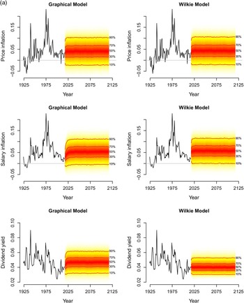
An additional check we can perform is to look at the (annualised) total returns of stocks and bonds over different horizons. We do this in Figure 9 for Model E6 and Figure 10 for the Wilkie model.
Plots of simulated share and Consols total returns from Model E6.

Plots of simulated share and Consols total returns from the Wilkie model.

As expected, the shape/sign of the bivariate correlation appears to be more stable for the graphical model than the Wilkie model. This is because we identified this type of long-run stable dependence as an objective for our models. An interesting outcome, however, is the mass placed by the graphical model on an extreme zone during the shorter horizons. Given the recent history of exceptional policy intervention by developed countries that exceeded the GDP of most countries in the world, this is not a surprising result. It is mainly driven by exceptionally low yields so that small absolute changes in yields can lead to very high returns. This feature does not appear in the Wilkie model, which may partly be because the Wilkie dynamics are more tightly constrained and do not allow the yields to frequently get pushed back down to the lower bound. In the graphical model, as the yields bounce away from a lower bound, they may be pushed back down by developments in other variables such as price inflation. This feature speaks to the ability of a simple graphical model with AR(1) dynamics and dependent innovations to also capture shorter-term risks.
5.4 A life insurance annuity example
We now consider a simulation example on a simple life insurance annuity contract. As the main purpose of this example is to highlight the stochastic variability of the underlying economic factors, we have used a simple Gompertz–Makeham model for force of mortality at age x: μ x = α β x . The estimated parameters are α = 0.00008 and β = 1.093, based on the England and Wales data from Human Mortality Database (https://www.mortality.org/) for ages 60–99 and years 1961– 2013. We have not modelled future mortality improvements and the uncertainties involved in future mortality projections.
Consider a portfolio of immediate life annuities of £1 payable annually in arrears (for a maximum of 40 years) sold to a cohort of 60-year-old individuals, all of whom follow the same mortality model as specified above. We assume that the assets are invested equally in bonds and equities; and rebalanced at the end of each year. Figure 11 shows the distributions of the price of the annuity based on the projected economic scenarios from Model E6 and the Wilkie Model.
Distribution of price of an immediate annuity of £1 payable annually in arrears (for a maximum of 40 years) sold to a cohort of 60-year-old individuals.

Both the distributions show similar characteristics, including right skewness and similar averages: £12.5 for Model E6 and £13 under the Wilkie Model. However, the dispersion or variability under Model E6 is higher. This is a direct consequence of the greater variability that can be observed in the bivariate heat maps of the Consols total return and share total return as shown in Figure 7.
6. Discussion
We have provided a step-by-step analysis of the data used to build a graphical dependence structure of the residuals from the simplest, but adequate, time series model of five variables. This has partly been for ease of exposition and partly to use the same data as applied in the benchmark paper. The use of a simple AR(1) model, which we have shown to be at least adequate for the current dataset, demonstrates the potential of graphical models to generate the rich structures required for long-term risk management applications. However, this does not preclude the possibility that actuaries may wish to develop more complex models of time series, with many more dimensions for their own applications. Extending the procedures demonstrated in this paper is straightforward in such cases. In most cases, such procedures would lead to intermediate models, between the relatively agnostic structure of the graphical models and the highly parameterised structure of a cascading model.
It is also possible to apply other graphical modelling techniques to focus on specific concerns, for instance, issues of non-Gaussianity or nonlinearity and high persistence in the time series. One of the insights we confirmed was that, as is well known from the macroeconomics and finance literature, a model that generates different regimes for correlation in good and bad times could improve the forecast distributions. Despite relying on a simple dynamic and a multivariate normal distribution for the innovations, the model captures some of these effects simply through the design of a suitably reduced form dependence structure. However, it is possible to model regime shifts directly in graphical models. Recent work on graphical models includes improvements in time series modelling (e.g. Wolstenholme & Walden, Reference Wolstenholme and Walden2015), in identifying separate subsamples (using, for instance, stratification as in Nyman et al. (Reference Nyman, Pensar and Corander2017)), and in jointly estimating the dependence structure and change points in time series using a single algorithm (Gibberd & Roy, Reference Gibberd and Roy2017).
Drton & Maathuis (Reference Drton and Maathuis2017) provide a useful overview of recent developments in graphical models, including directed graphs. The use of directed graphs in cases where the (statistical) causality is clear and well established may assist in improving graphical models, but also risks exposing the modeller to regime shifts. When the economic causality is not fully established, a directed graph may increase the wrong way risk of certain scenarios more than an undirected graph, which is another reason to be cautious about additional assumptions in long-term risk modelling.
7. Summary and conclusions
We have attempted to demonstrate the transparency, flexibility and portability of graphical models for developing an ESG. There are undoubtedly other, more structural, models in the large VAR literature that could effectively capture the joint dynamics of variables. However, such models must by necessity be tightly parameterised and ultimately require some dimension reduction approach as the number of variables increases. Instead, we have seen that the simple model with AR(1) dynamics combined with graphically modelled innovations can generate rich and reasonable distributions for use in long-term risk management.
The fitted model performs comparably to the established benchmark and has the additional advantage of easy portability to new datasets, transparency and flexibility. Although for ease of exposition, we have considered only five UK economic variables in this paper, the model can easily accommodate extensions to a wider range of economic variables and also for many different countries. We do not claim that this model is superior compared to other available models, as all models have their strengths and limitations.
Our broader objective in this paper is to promote the use of statistical graphical modelling approach for actuarial functions. We envisage that the techniques outlined in this paper can be modified and adapted to a wide range of actuarial applications, including modelling of cause-specific mortality and morbidity rates; investigation of insurance claims based on a range of insurance risk rating categories; analysing the relationships between different sources of risks for quantifying risk-based solvency capital requirements; to suggest a few possibilities.
As access to ever larger datasets improves, actuarial researchers and practitioners will need to seek out and develop ever more innovative and sophisticated tools and techniques to analyse data and extract the most relevant information from these extensive datasets for decision making purposes. In this paper, we demonstrated the usefulness of one such dimension reduction technique in the form of statistical graphical models.
Author ORCID
Pradip Tapadar, http://orcid.org/0000-0003-0435-0860
Acknowledgments
We are extremely grateful to David Wilkie for freely sharing his data and advice on numerous occasions. We are also grateful to Doug Andrews, Stephen Bonnar, Lori Curtis, Melania Nica, Bruce Porteous and Vaishnavi Srinivasan for reading the paper and providing helpful comments. We would also like to thank participants at the Mathematical and Statistical Methods for Finance and Actuarial Science Conference (2018) for comments. This project has benefited from funding provided by the Institute and Faculty of Actuaries (IFoA) and we are grateful for their support.
Disclaimer
The views expressed in this publication are those of the authors and not necessarily those of the IFoA. The IFoA do not endorse any of the views stated, nor any claims or representations made in this publication and accept no responsibility or liability to any person for loss or damage suffered as a consequence of their placing reliance upon any view, claim or representation made in this publication. The information and expressions of opinion contained in this publication are not intended to be a comprehensive study, nor to provide actuarial advice or advice of any nature and should not be treated as a substitute for specific advice concerning individual situations.