



1. Introduction
The stability of hierarchical triples is not only an intriguing problem but also highly important in terms of understanding several astronomical phenomena. For instance, understanding gravitational wave emission mechanisms, the stability of exoplanetary system, and N-body simulations of dense star cluster.
Here, we describe the design of traditional stability criteria. Let Q is the ratio of outer peri-center distance
 $q_\mathrm{out}$
and inner semi-major axis
 $a_\mathrm{in}$
, i.e.,
 \begin{equation} Q = \frac{q_\mathrm{out}}{a_\mathrm{in}} = \frac{a_\mathrm{out}(1-e_\mathrm{out})}{a_\mathrm{in}}, \end{equation}
where
 $a_\mathrm{out}$
is the semi-major axis of inner orbit and
 $e_\mathrm{out}$
is the eccentricity of outer orbit. Traditional stability criteria define the minimum value of Q using semi-analytical or numerical approach (e.g., Harrington Reference Harrington1977; Eggleton & Kiseleva Reference Eggleton and Kiseleva1995; Mardling & Aarseth Reference Mardling and Aarseth2001; Mylläri et al. Reference Mylläri, Valtonen, Pasechnik and Mikkola2018; Vynatheya et al. Reference Vynatheya, Hamers, Mardling and Bellinger2022). Such minimum Q value,
 $Q_\mathrm{crit}$
, is a function of the initial orbital elements of triples, i.e.,
 $Q_\mathrm{crit} = Q_\mathrm{crit} (m_1, m_2, m_3, a_\mathrm{in}, a_\mathrm{out}, e_\mathrm{in}, e_\mathrm{out}, I,...)$
. If
 $Q\gt Q_\mathrm{crit}$
, the triple is regarded as stable, otherwise unstable.
However, there are critical issues for prediction accuracy within ambiguous parameter space, called mixed-region that stable and unstable systems coexist (e.g., Dvorak Reference Dvorak1986). In 6-dimensional phase space, the stability and instability boundary of triple seems to be fractal-like structure (Trani et al. Reference Trani, Leigh, Boekholt and Portegies Zwart2024), so it is fundamentally challenging to predict stability only using initial condition.
Lalande & Trani (Reference Lalande and Trani2022, hereafter LT22) is the first work to avoid such difficulties in the mixed-region. They did hundreds of N-body simulation of hierarchical triples and train machine learning (ML) model to predict stability using first
 $10^5 P_\mathrm{in}$
orbital evolution. Their ML model shows the Area under the Receiver Operating Characteristic curve (AUC) of 0.95, not knowing the nature of instability of triples.
In this work, we conducted N-body simulations of hierarchical triples and analyze the orbital evolution using Fourier analysis in terms of orbital periodicity (e.g., Binney & Spergel Reference Binney and Spergel1982). This contribution summarizes our previous work (Iwakura et al. Reference Iwakura, Funato and Makino2025, hereafter I25).
2. Initial condition and numerical method
We considered four prograde cases and four retrograde cases. The selected Q values are
 $Q=3.73, 3.75, 3.77, 3.80$
for prograde cases and
 $Q=2.52, 2.55, 2.58, 2.60$
for retrograde cases. These Q values are about 5-15% below the
 $Q_\mathrm{crit}$
of MA01 stability criterion, which means our triples are regarded as unstable by MA01 condition. Orbital elements except for outer semi-major axis are fixed as figure 1. Once Q values are decided, we can calculate Q value using Q definition equation (1). For each Q values, we prepare 1000 initial conditions differentiating node (
 $\omega$
) and orbital phases (
 $M_\mathrm{out}$
; mean anomaly). Thus, the total number of initial condition is
 $8\times1000=8000$
.
Initial parameter. In our coplanar case, we set
 $\Omega_\mathrm{in} = \Omega_\mathrm{out} = 0$
, since the longitude of the ascending nodes are not defined for coplanar triples.

Table 1 Long description
A table with one row and eight columns. The columns are labeled as follows: m1, m2, m3, a_in, e_in, e_out, ω_in, ω_out, M_in, M_out. The row contains the following values: 0.5, 1, 0.5, 0.25, 0, U[0,1), U[0,1), U[0,1). The table presents initial parameters for a coplanar case, with specific values and uniform distributions for certain parameters.
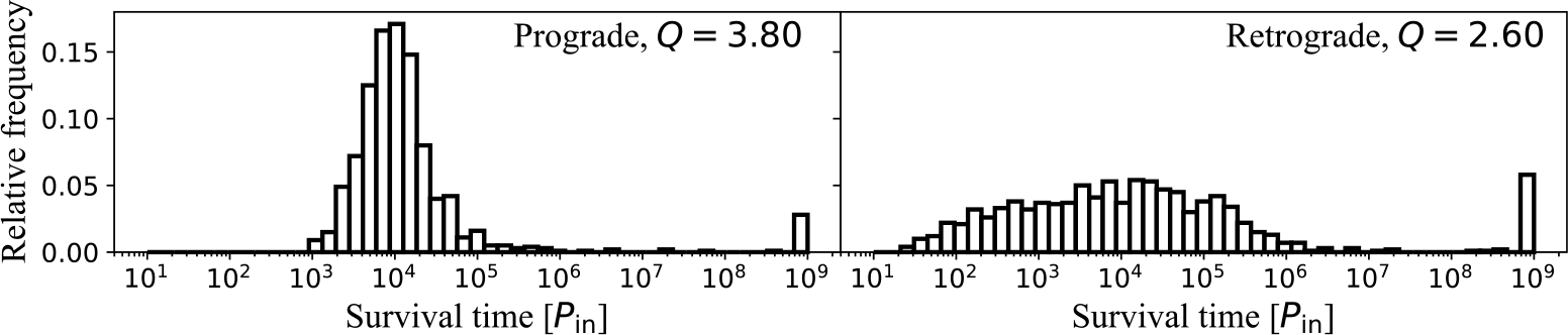
Example of lifetime distribution of triples.

For N-body integrator, we make use of the combination of Algorithmic regularization (AR; Preto & Tremaine Reference Preto and Tremaine1999; Mikkola & Tanikawa Reference Mikkola and Tanikawa1999) and 6th order symplectic formula (Yoshida Reference Yoshida1990). AR is a regularized integrator so it is suitable for long-term integration of few-body systems. AR integrator library is freely available in https://github.com/lwang-astro/SDAR (Wang et al. Reference Wang, Nitadori and Makino2020).
3. Results
3.1. The lifetime distribution of triples with same Q value
Figure 1 depicts the lifetime distribution of triples with same Q value,
 $Q=3.80$
for prograde cases and
 $Q=2.60$
for retrograde cases. Even if the systems have same Q value, the difference of initial nodes and phases affect the lifetime of triples, as mentioned in Hayashi et al. (Reference Hayashi, Trani and Suto2022, Reference Hayashi, Trani and Suto2023). This fact reveals that the Q-based stability criteria is inappropriate in the mixed-region, because normally such criteria does not consider the dependence of initial nodes and phases. Even if one try to investigate the dependencies of nodes and phases, the chaotic nature of triples will prevent from doing so.
3.2. The periodicity analysis using Fourier analysis
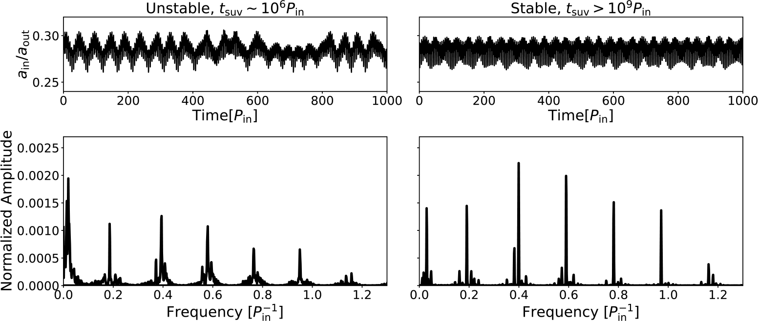
We compare stable and unstable orbits as seen in figure 1, especially in terms of orbital periodicity using Fast Fourier Transform (FFT). Figure 2 depicts two examples of semi-major axes ratio (
 $a_\mathrm{in}/a_\mathrm{out}$
) and its FFT results, which is the spectrum of
 $a_\mathrm{in}/a_\mathrm{out}$
for initial
 $\sim10^3$
orbits. Even though both of them are for
 $Q=2.60$
retrograde orbits, the survival time
 $t_\mathrm{suv}$
and the spectrum are different. This is because the initial nodes and phases are different. Traditional Q-based stability criteria cannot tell them apart, as showed in figure 1.
Comparison between semi-major axes ratio and FFT results. These two cases are for
 $Q=2.60$
retrograde orbits, changing initial node
 $\omega_\mathrm{out}$
and phases
 $M_\mathrm{in}, M_\mathrm{out}$
. Since FFT requires the number of data to be a power of 2,
 $2^{13}=8192$
data points are used. Actually, this extracted data corresponds to initial
 $819.2P_\mathrm{in}$
, because our output time interval is set to
 $0.1P_\mathrm{in}$
.

Figure 2 Long description
The image contains four graphs, two line graphs on the top row and two bar graphs on the bottom row. The top row compares unstable and stable orbital systems over time. The left line graph shows the unstable system with the ratio of semi-major axes on the vertical axis and time on the horizontal axis. The right line graph shows the stable system with the same axes. The bottom row displays the normalized amplitude of the systems. The left bar graph corresponds to the unstable system, and the right bar graph corresponds to the stable system. Both bar graphs have frequency on the horizontal axis and normalized amplitude on the vertical axis. The unstable system shows more variability over time and frequency compared to the stable system.
From careful observation, we found that stable systems tend to have smaller continuous components and clear peaks. The clearness of the peaks means the periodicity of orbital evolution, so stable systems exhibit a more periodic manner even in first
 $\sim 1000 P_\mathrm{in}$
.
3.3. Quantification of orbital periodicity using FFT results
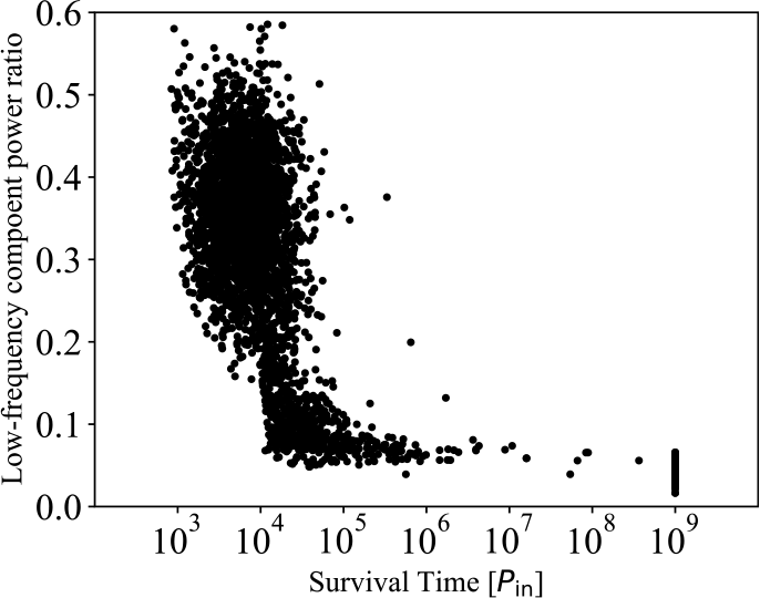
In figure 2, unstable orbit has larger peak near 0 frequency than stable one. We refer this peak as low-frequency component and define the periodicity as the ratio of the amplitude of the low-frequency component to the total power of FFT spectrum. Figure 3 shows the correlation between the survival time and the total power of low-frequency components.
The correlation between the survival time and the total power of low-frequency components. All of the dots represent four types of prograde cases. The vertical axis shows the sum of the components in the range 0-0.09
 $P_\mathrm{in}^{-1}$
. For retrograde cases, see figure 7 in I25.

The long-period variations correspond to fluctuations on the timescale of the synodic period between the outer and inner orbits, and are considered to result from the combined effects of mean motion resonances and secular perturbations. For a system to remain stable over long timescales within the mixed-region, these variations need to be relatively small. Using this correlation as the stability criteria for coplanar triples shows a good performance in terms of precision. For detailed information, see section 3.3 in I25.
4. Discussion and ongoing work
In this study, we present a novel method for predicting the stability of hierarchical triple systems, showing that traditional criteria are insufficient within the chaotic mixed-region. We found that a system’s long-term stability is strongly correlated with the periodicity of its orbital evolution, which is evident within the first 1000 inner orbital periods. By using a Fourier analysis, we demonstrate that stable systems have distinct frequency peaks, while unstable systems possess significant low-frequency components. Quantifying the power of these low-frequency components allows for a highly accurate prediction of whether a system will remain stable, far outperforming previous methods.
Currently, we are attempting to apply the same method to inclined cases by examining the FFT of the time evolution of the semi-major axes ratio. We are also exploring whether ML approach of the FFT results can enable more accurate classification, as LT22 did. When there are inclination between inner and outer orbit, the orbital evolution becomes more complex than coplanar cases because of von Zeipel-Lidov-Kozai effect (von Zeipel Reference von Zeipel1910; Lidov Reference Lidov1962; Kozai Reference Kozai1962). However, when analyzing the FFT results of semi-major axes ratio, the same correlation pattern is found. We are currently investigating whether a ML approach can predict stability in combination with our present method using FFT.

 Ωin=Ωout=0
 Q=2.60
 ωout
 Min,Mout
 213=8192
 819.2Pin
 0.1Pin
 Pin−1


