Introduction
The tides of the polar oceans, and especially the tides under the great Antarctic ice shelves, are inadequately known (Stammer et al. Reference Stammer, Ray, Andersen, Arbic, Bosch and Carrère2014, Ray et al. Reference Ray, Loomis, Luthcke and Rachlin2019). Satellite altimetry, which has led to remarkably accurate deep-ocean tidal models in lower latitudes, has been less successful in polar regions. All satellites overflying polar latitudes suffer unfavourable aliasing properties for solar tides, and ice cover hampers analysis of radar returns, although progress is slowly being made (Padman et al. Reference Padman, Erofeeva and Fricker2008, Zaron Reference Zaron2018). To help such efforts, good in situ measurements of tides are invaluable. Moreover, in situ measurements allow fine details of the ocean's tidal response to be studied in ways not generally possible with aliased satellite data. For the floating Antarctic ice shelves, a tidal archive of in situ data is slowly being constructed based on the analysis of tide observations extracted from high-rate Global Positioning System (GPS) - or, more generally, Global Navigation Satellite Systems (GNSS) - measurements; see, for example, work by King & Aoki (Reference King and Aoki2003) and King et al. (Reference King, Padman, Nicholls, Clarke, Gudmundsson, Kulessa and Shepherd2011).
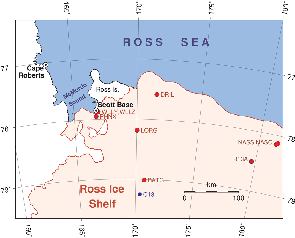
This paper adds to these efforts by analysing elevation time series from a number of GPS stations on the north-western Ross Ice Shelf (Fig. 1). Most of these stations have been established only in the past few years, but the time series are now sufficiently long to yield useful tidal information. We also take the opportunity to reanalyse two long time series of more conventional data collected at two permanent stations maintained by New Zealand: Scott Base, on the southern tip of Ross Island, which adjoins the ice shelf, and Cape Roberts, on the western boundary of McMurdo Sound along the coast of Victoria Land. These data provide context for the shorter GPS time series, including necessary information for a response analysis of three older, very short GPS time series.
Location of the study area. Cape Roberts and Scott Base are permanent tide-gauge locations, maintained by New Zealand. Red circles mark the locations of high-rate GPS positioning time series. The three GPS sites in the east are very short time series from MacAyeal et al. (Reference MacAyeal, Brunt and King2008). At station C13, marked by the blue dot in the south, 29 days of tidal gravity measurements were collected in 1974 (Williams & Robinson Reference Williams and Robinson1980).

The earliest sustained observations of tides in this region were obtained just after the turn of the twentieth century during the famous polar expeditions of Robert Scott and Ernest Shackleton. Those measurements were confined to the southernmost point of Ross Island along the south-eastern corner of McMurdo Sound, where the major polar expeditions were based. Present-day McMurdo Station and Scott Base are in the same vicinity. Reports and analyses based on these early measurements were published by Darwin (Reference Darwin and Darwin1907, Reference Darwin1910) and Doodson (Reference Doodson and Lyons1924). More recent observations date from the International Geophysical Year (IGY) and thereafter, with subsequent discussions by Gilmour et al. (Reference Gilmour, Macdonald and van der Hoeven1962) and Heath (Reference Heath1971). Gravimeter measurements of the tides were obtained near the edge of the eastern sector of the Ross Ice Shelf (78°S, 162°W) for 1 month during the IGY (Thiel et al. Reference Thiel, Crary, Haubrich and Behrendt1960). An extensive campaign of gravimeter tide measurements across the whole ice shelf was reviewed by Williams & Robinson (Reference Williams and Robinson1980).
Darwin's Reference Darwin and Darwin1907 report was based on measurements made by the Discovery expedition when the ship was frozen in by ice from early 1902 to early 1904. The crew had measured the tide by running a wire through winter ice to a weight on the sea floor, first to a tripod sitting on the ice surface some 200 m from the ship, and later to a gauge affixed to the deck of the ship itself, making small corrections for the trim and list of the ship. A quick glance at the recordings showed the dominance of diurnal tides, with unusually small semidiurnal tides. Darwin's harmonic analysis quantified this, finding comparable amplitudes for O1 and K1 that were almost five times larger than those of M2. Darwin noticed a clear seasonal variation in both the amplitude and phase of M2, but not in the larger diurnal constituents. This appears to have been the first report by anyone of a seasonal change in tidal constants, currently a topic of great interest (e.g. Kang et al. Reference Kang, Foreman, Lie, Lee, Cherniawsky and Yum2002, Müller Reference Müller2012, Müller et al. Reference Müller, Cherniawsky, Foreman and von Storch2014, Wang et al. Reference Wang, Pan, Jin and Lv2020). We return to this point below.
New tidal analyses are reported in the following two sections for Cape Roberts and Scott Base. Harmonic constants at each of these stations have been reported previously using shorter time series (Goring & Pyne Reference Goring and Pyne2003), but the extended data allow some interesting features to be brought out. One of them is seasonal variability, noted above. Another is the detected presence of small diurnal and semidiurnal tides generated by the third-degree terms (Cartwright & Tayler Reference Cartwright and Tayler1971) in the moon's astronomical potential. These are caused ultimately by the fact that the potential's two-sided tidal bulge is not perfectly symmetrical, being slightly larger on the side with the moon and slightly smaller on the other. The resulting third-degree constituents are very small, typically only a few millimetres, and they require long time series to separate from conventional tides. Although small, they give unique insight into the ocean's response to large-scale forcing (e.g. Cartwright Reference Cartwright1975, Woodworth Reference Woodworth2019). They are clearly observable at Cape Roberts and Scott Base, so we devote some effort to their careful determination. Subsequent sections are devoted to tidal analyses of the GPS data.
Tides at Cape Roberts
The tide gauge at Cape Roberts (77°02'S, 163°11′E) is maintained by Land Information New Zealand. It is a pressure sensor. Beginning in 2011, the released data files include atmospheric pressure and seawater temperature as well as subsurface pressure. Analysis of the air pressure data reveals (as one might expect) only small amplitudes for diurnal and semidiurnal atmospheric tides, the largest being S2 at ~9.5 Pa, equivalent to ~0.95 mm in sea-surface height. The amplitude of the M2 atmospheric tide is < 2 Pa. In light of these small amplitudes, the atmospheric pressure data will be ignored below and the Cape Roberts subsurface pressures treated as measurements of solely the ocean tide.
The time series extends from November 1990 through to the end of 2018, although with three significant gaps of a year or more. The longest gap, across all of 2010 and most of 2011, was preceded by a period of large drift in the recorded mean level beginning in August 2009. Those data have been discarded. When the time series restarted in November 2011, there is a clear vertical offset, which is estimated at ~28.2 cm (the newer data reporting higher sea levels).
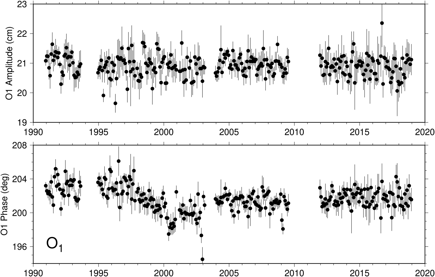
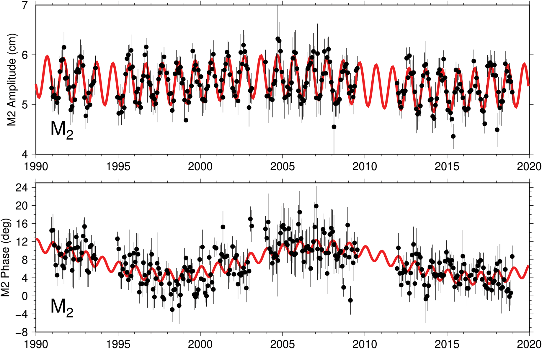
The tidal constants reported below are based on least-squares analysis of the whole 1990–2018 time series. It is almost always beneficial, however, to analyse such a long time series in a preliminary fashion by partitioning it and analysing shorter segments. Figures 2 & 3 show monthly estimates of the amplitudes and phase lags of O1 and M2, respectively. The O1 phase lags show a decreasing trend over the interval 1996–2000, with a slight recovery and relatively constant phases before and after. In older data, one might naturally suspect instrument problems when tidal phases change, but in modern measurements, especially in this region, environmental changes (e.g. possible changes in ice cover somewhere in the region) seem just as probable, perhaps more so. Diurnal constituents Q1 and K1 hint at similar changes (not shown), although their phases are much noisier owing to small amplitudes (for Q1) or possible perturbations from nearby constituents (such as S1 for K1).
Monthly estimates of the (top) amplitudes and (bottom) Greenwich phase lags of the O1 constituent at Cape Roberts. Standard errors are determined from the error covariance matrix, scaled to account for the residual variance near the O1 frequency. The cause of the phase decay between 1996 and 2000 is unknown.

Monthly estimates of the (top) amplitudes and (bottom) Greenwich phase lags of the M2 constituent at Cape Roberts. Red curves represent sinusoids of periods 1 year and 18.6 years, fitted to the monthly data by weighted least squares. Annual variations are especially pronounced in amplitude (cf. Darwin Reference Darwin and Darwin1907). One contributor to the 18.6 year variations is the possible presence of a significant non-linear compound tide KO2, at the same frequency as M2 but with much larger nodal modulations.

The M2 phases in Fig. 3 also decrease during 1996–2000, and by amounts roughly double the changes in O1, as would occur with timekeeping errors. However, the M2 phases are slowly changing throughout the whole time series, and they can be reasonably well fit by a sinusoid of period 18.6 years (cf. red line in Fig. 3), suggesting that the standard nodal modulations that were applied during harmonic analysis are inadequate. In this case, given the small amplitude of M2, a possible contributor to these changes is the presence of the non-linear compound constituent KO2, whose frequency is identical to the M2 frequency. The non-linear KO2 has a nodal phase modulation of comparable magnitude, but of opposite sign, to the M2 phase modulation; it could either add or subtract from the standard M2 modulation depending on whether M2 and KO2 are in or out of phase. The 18.6 year fit in Fig. 3 is not perfect, and in fact the phases over 1996–2000 still appear anomalously low, as with O1.
In Fig. 3, the M2 amplitudes clearly display the seasonal oscillations first noticed by Darwin (Reference Darwin and Darwin1907). Similar oscillations occur in the M2 phases, although these are smaller.
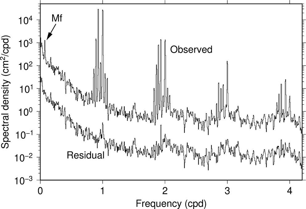
Notwithstanding the possible instrumental or environmental effects behind the noted phase changes, we estimated harmonic constants for Cape Roberts from the whole series. The number and selection of constituents were determined in part by repeated examination of spectra of tidal residuals, computed over the interval 2006–08, which has no data gaps; any evident tidal peaks in the residual spectrum would indicate one or more overlooked constituents, which were subsequently included in a new inversion. The Cape Roberts spectrum, before and after tidal analysis, is shown in Fig. 4 up through the quarter-diurnal band (higher-frequency bands appear to have only weak constituents, with amplitudes all < 1.2 mm).
Spectra of observed sea level and computed tidal residuals at Cape Roberts, from data over a ~3 year interval from 26 January 2006 to 30 December 2008 without data gaps. The residual spectrum is offset for display purposes. The diurnal band dominates all other tidal bands. A conspicuous peak of the fortnightly Mf constituent is evident in the long-period band. The largest peak in the terdiurnal band occurs at the S3 group. A large peak near M2 is prominent in the residual spectrum, presumably owing to the M2 variability seen in Fig. 3.

In Fig. 4, an isolated and conspicuous peak in the residual spectrum occurs at Fourier frequency 1.933 cycles per day (cpd), which coincides approximately with the frequency of M2. This residual peak is consistent with the variability of M2 seen in Fig. 3, which effectively spreads energy away from the main tidal line. An attempt to estimate both M2 and KO2, possible only owing to their very different nodal modulations in amplitude, successfully removed nearly all of this residual peak, but the estimates themselves are overly correlated and therefore not reliable. (See the discussion by Amin (Reference Amin1985) of similar attempts to disentangle coupled linear and non-linear constituents.)
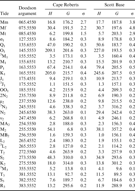
The major tidal constituents at Cape Roberts are listed in Table I, and a more complete table is included in the Supplemental Material. The variable σ denotes the standard error in in-phase or quadrature components. Corresponding standard errors in amplitude H and phase G are σ and σ/H, respectively, assuming σ ≪ H; otherwise, errors in amplitude and phase are more complicated functions of σ (Munk & Cartwright Reference Munk and Cartwright1966, their appendix B). These standard errors have been computed from the error covariance after accounting for the residual spectral densities surrounding each frequency. They have been checked by solving for tides in each of the n years and computing the standard deviation of these yearly estimates divided by √n. The two approaches give general agreement except near constituents such as N2, where the yearly analyses cannot account for the presence of third-degree tides (see below).
Selected tidal constituents estimated at Cape Roberts and Scott Base.

Amplitude H in mm; Greenwich phase lag G in degrees; standard error σ in mm.
For consistency, a superscript has been applied to M3, although this is unnecessary, as no second-degree tide can occur in the terdiurnal band.
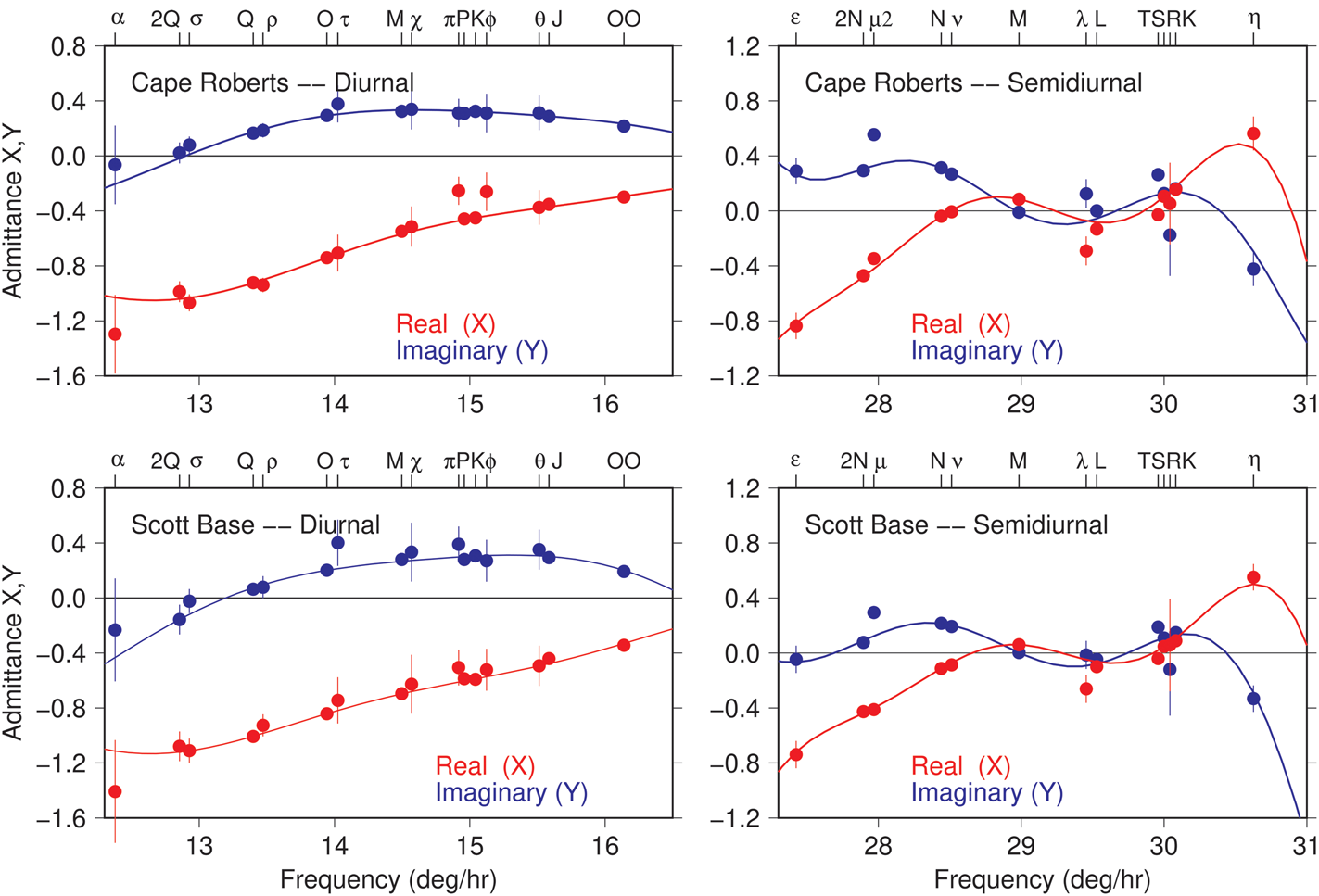
The diurnal and semidiurnal tidal admittances (relative to the generating potential amplitudes of Cartwright & Tayler Reference Cartwright and Tayler1971) are shown in Fig. 5. The smooth curves shown in Fig. 5 represent low-order Fourier series determined by weighted least-squares fits to the individual tidal harmonics. The diurnal-band admittances are smooth, with little curvature across the band. The semidiurnal admittances are far less so, dropping to near-zero amplitudes in the frequency band between M2 and S2. Although Table I indicates M2 to be the largest semidiurnal constituent, its amplitude is still only 5.4 cm, and it is considerably suppressed relative to constituents nearer the edges of the band. The semidiurnal admittances show at least one constituent, μ2, affected by non-linear perturbations and thus offset from the smooth curves. In fact, constituent μ2, which coincides with the compound 2MS2, is similarly perturbed in many ports throughout the global ocean. The jitter in the S2 group is usually caused mainly by radiational perturbations (Cartwright & Ray Reference Cartwright and Ray1994). These admittance curves prove useful below, when a response analysis is employed on three very short time series.
Tidal admittances Z = X + iY for Cape Roberts (top row) and Scott Base (bottom row), in the diurnal band (left) and semidiurnal band (right). Circles denote admittances estimated by harmonic analysis (Table SI). Smooth curves are low-order Fourier series determined by weighted least-squares fits to the individual constituents (excluding ones clearly affected by non-linear perturbations, such as μ2). Admittances at the two tide gauges, located on opposite sides of McMurdo Sound, are very similar. Subscripts on constituent names (upper axes) have been suppressed to save space.

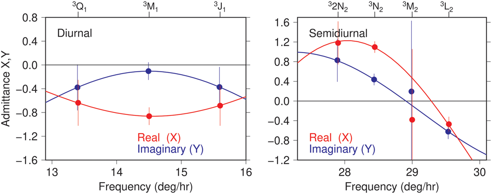
An advantage of a long time series, in addition to improved precision of tidal estimates, is the separation of harmonics with close frequencies. The often-neglected tidal constituents generated by the third-degree terms in the tide-generating potential generally require at least nine years of data to separate them from the usual second-degree tides. A number of third-degree tides have been determined for Cape Roberts and are included in the supplemental Table SI. The largest constituents are 3N2 in the semidiurnal band with amplitude 4.6 mm and 3M1 in the diurnal band with amplitude 3.5 mm (where a leading superscript ‘3’ has been added to distinguish them from second-degree tides). Although small, these amplitudes are actually fairly large for third-degree tides. The amplitude of 3M1 is in good agreement with the recent numerical model of Woodworth (Reference Woodworth2019), although the phases differ by ~40°. The third-degree admittances are shown in Fig. 6. Within error bars, the diurnal admittance could be considered constant across the whole band. Similarly to the second-degree tides, the third-degree semidiurnal admittance has far more curvature, with very small amplitudes in the centre of the band near M2 (the error bars on 3M2 itself are too large to determine this, but the semidiurnal admittance, as interpolated between the well-determined constituents 3N2 and 3L2, is clearly near zero). The shapes of the second-degree and third-degree admittances, however, are otherwise dissimilar, as must be expected from the very different astronomical forcing.
Tidal admittances at Cape Roberts for constituents generated by the third-degree terms in the astronomical potential.

Tides at Scott Base
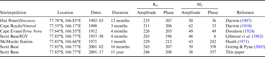
New Zealand's Scott Base (77°51′S, 166°46′E) sits near the southernmost point of Ross Island (Fig. 1). Most of the historical tide measurements in this region of Antarctica have in fact occurred along the coast of Ross Island, including those of the Scott and Shackleton expeditions. A compilation of those historical data, plus any available modern measurements, is given in Table II. Only the bottom two rows of Table II, which are based on relatively long time series, show good agreement. The M2 phase of Heath (Reference Heath1971) is clearly suspect. Note that differences between the modern and the early twentieth-century measurements may be due partly to location, as the older data were obtained more towards the western part of the island. For example, the numerical model of Lyard et al. (Reference Lyard, Lefevre, Letellier and Francis2006) predicts K1 at the Nimrod position to be 16 mm smaller, and M2 to be 8 mm larger, than the corresponding tides at Scott Base, which does explain part of the discrepancy between the modern estimates and those of Darwin (Reference Darwin1910).
Tide measurements at Ross Island.

Amplitudes in mm; Greenwich phase lags in degrees.
The data analysed here are from a tide gauge that has been operational since 2001. See the description by Goring & Pyne (Reference Goring and Pyne2003) for the instrumental setup. Over the past two decades, the time series shows many data gaps, the longest being a nearly 5 year span covering most of 2006–10. In total, only 54% of the days since 2001 have valid data. (These statements describe data archived at the University of Hawaii Sea Level Center. Additional data apparently exist but are not yet in international archives.)
Monthly tidal estimates (not shown) display variability comparable to that seen at Cape Roberts. Harmonic analysis over the whole post-2001 period yields constants listed in Table I (with more complete tabulation in Table SII). Diurnal and semidiurnal admittances at Scott Base are shown in the lower panels of Fig. 5, and they are very similar to the admittances at Cape Roberts, including the non-linear perturbation in μ2. Admittances for third-degree tides (not shown) are also similar to those of Cape Roberts.
Harmonic constants in Table I compare fairly well with those previously obtained by Goring & Pyne (Reference Goring and Pyne2003). The largest discrepancy is probably N2, where the results here find amplitude H = 29.4 ± 0.2 mm and phase G = 242.4° ± 0.4°, whereas Goring & Pyne (Reference Goring and Pyne2003) give H = 26.7 ± 0.7 mm and G = 248.9° ± 1.5°. The difference is almost certainly due to the presence of the third-degree constituent 3N2, with amplitude 3.7 mm, which could not be separated from N2 in the short (471 day) time series available to Goring & Pyne (Reference Goring and Pyne2003). These two waves beat with a 9 year periodicity, and during 2001 and early 2002 (when Goring & Pyne Reference Goring and Pyne2003 collected data), the combination leads to a reduced amplitude and advanced phase lag, consistent with the above two comparisons. All of the GPS time series discussed below are much shorter than nine years, so they will be susceptible to similar errors from third-degree tides.
Tides at recent GPS stations
Tidal analysis of high-rate (i.e. hourly or faster) GNSS position data is today a well-established tool for determining tides on floating ice (e.g. King et al. Reference King, Padman, Nicholls, Clarke, Gudmundsson, Kulessa and Shepherd2011). This section describes results obtained from tidal analysis of high-rate data at five sites. All data were extracted from the comprehensive GPS database maintained at the Nevada Geodetic Laboratory (NGL) of the University of Nevada, Reno (Blewitt et al. Reference Blewitt, Hammond and Kreemer2018). The NGL elevation solutions were obtained with Jet Propulsion Laboratory (JPL) GipsyX software (Bertiger et al. Reference Bertiger, Bar-Sever, Dorsey, Haines, Harvey and Hemberger2020), using prior orbit and clock solutions produced at JPL (Repro3.0). Final data had 5 min sampling.
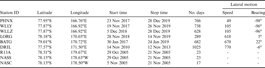
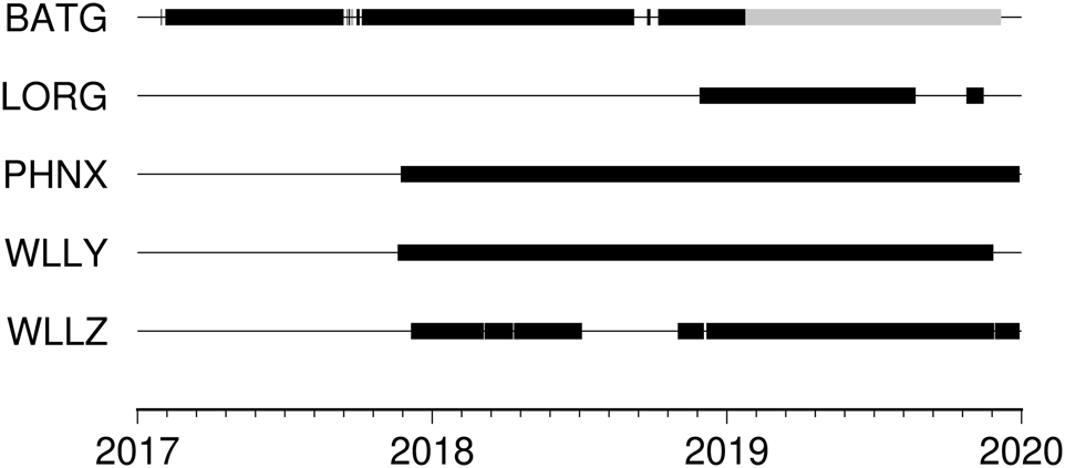
The stations analysed here are summarized in Table III, their locations are depicted in Fig. 1 and the times of data availability are shown in Fig. 7. Stations WLLY, WLLZ, PHNX and LORG were installed using fairly standard protocols for GPS deployments on ice. Each antenna was installed on a Rohn tower. A 0.5 m2 plywood sheet, containing three holes to accept the three tower legs, was buried horizontally in ~50 cm of snow, with the antenna then sitting ~2–3 m above the snow surface. Stations WLLY and WLLZ were separated by only ~40 m, and as Fig. 7 indicates, data were recorded contemporaneously, except for a gap in WLLZ. Station PHNX is also in close vicinity. The tidal constants for these three stations are therefore expected to be approximately equal. Station BATG used similar instrumentation (GPS receiver and antenna), but was mounted on a pre-existing 30 m tower that is used to measure atmospheric data (Lazzara et al. Reference Lazzara, Weidner, Keller, Thom and Cassano2012, their fig. 16).
GPS stations analysed.

Data for the last three stations are from MacAyeal et al. (Reference MacAyeal, Brunt and King2008) and Brunt et al. (Reference Brunt, King, Fricker and MacAyeal2010).
Lateral speed in m yr-1; bearing degrees east of north.
Timelines showing the availability of high-rate GPS solutions from Blewitt et al. (Reference Blewitt, Hammond and Kreemer2018). The grey segment of station BATG denotes suspect data.

Owing primarily to telemetry restrictions, all of the stations, including those still currently operating, tracked only the GPS constellation. For tidal studies, the difficulties in reliable estimation of K1 and K2 from GPS are well known (King Reference King2006), and recent work with other GNSS systems shows promise for alleviating these problems (Matviichuk et al. Reference Matviichuk, King and Watsonin press). For now, however, GPS is all that is available at these stations.
According to their documentation, Blewitt et al. (Reference Blewitt, Hammond and Kreemer2018) applied a prior model for ocean tidal loading based on the FES2004 ocean tide model of Lyard et al. (Reference Lyard, Lefevre, Letellier and Francis2006). This was done following the algorithms distributed by the International Earth Rotation and Reference Frames Service (IERS), by which 11 constituents are explicitly computed and other linear constituents in the semidiurnal, diurnal and long-period bands are inferred. Constituents of higher species or non-linear compound tides are therefore not corrected for crustal loading by these algorithms.
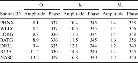
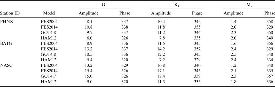
In the series of finite-element assimilation models produced by Lyard's group, the FES2004 model is at least two generations old, so the load tide computed from it may not be the best. Nonetheless, analysis of Gravity Recovery and Climate Experiment (GRACE) range-rate data suggests FES2004 is possibly no worse in this region of the Antarctic than other available global models (Stammer et al. Reference Stammer, Ray, Andersen, Arbic, Bosch and Carrère2014, Ray et al. Reference Ray, Loomis, Luthcke and Rachlin2019). For example, FES2012 appears more accurate for O1 but less accurate for K1. Fortunately, the load tides here are fairly small. Table IV lists the FES2004 load-tide amplitudes and phases for the three major constituents O1, K1 and M2 at our GPS stations (closely neighbouring stations not included), and Table V compares other models at three locations. According to Table V, the largest discrepancy among models is 8 mm (for both K1 and O1 at BATG). Any errors in these prior load-tide adjustments, of course, map directly into the subsequent ocean-tide estimates. In due course, as load-tide models improve through better knowledge of Antarctic ocean tides, our GPS ocean-tide estimates can be adjusted accordingly.
Load tides removed during GPS processing, major constituents.

Load-tide amplitudes in mm; Greenwich phases in degrees.
Load tides based on the FES2004 ocean-tide model (Lyard et al. Reference Lyard, Lefevre, Letellier and Francis2006).
Comparison of load-tide models.

Load-tide amplitudes in mm; Greenwich phases in degrees.
The various ocean-tide models are from Lyard et al. (Reference Lyard, Lefevre, Letellier and Francis2006), Ray (Reference Ray1999) and Taguchi et al. (Reference Taguchi, Stammer and Zahel2014), with updates.
A few issues with these new GPS data from the Ross Ice Shelf deserve mentioning. Station WLLZ's antenna was raised on 28 November 2019. We estimated this offset to be ~151 cm and corrected the data accordingly. Secondly, the BATG GPS receiver began to fail in January 2019. This failure coincided with orders of magnitude more cycle slips than the earlier records. Because we need kinematic solutions for tides and estimating thousands of extra cycle parameters yields poorly constrained solutions, we have opted to use only the earlier BATG data collected between January 2017 and January 2019.
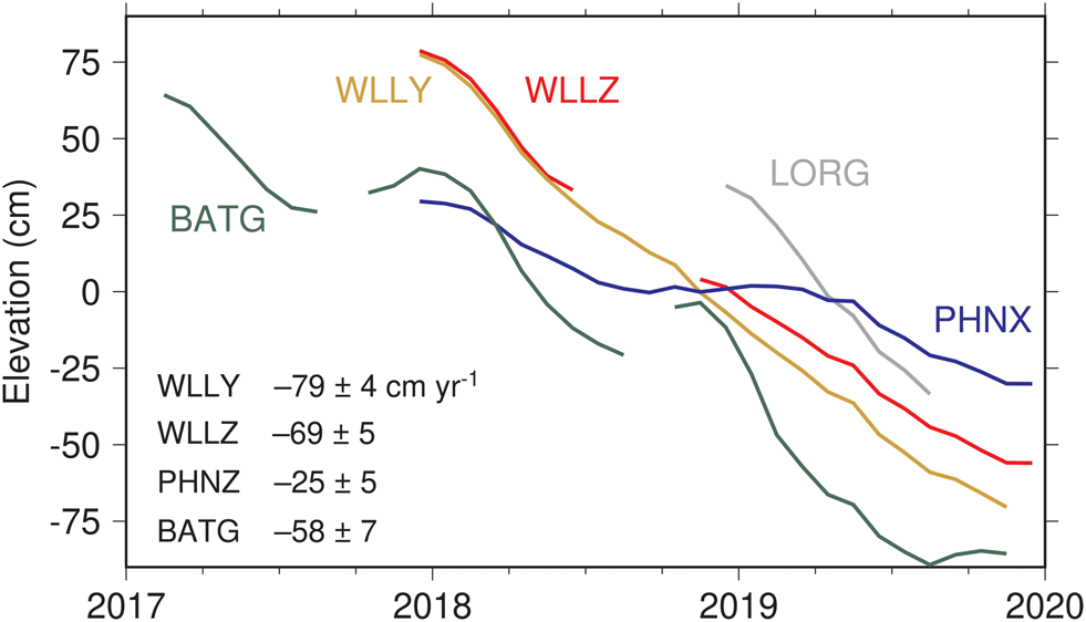
The elevation data for all of these stations reveal conspicuous negative trends. Figure 8 shows monthly mean elevations at each station, and the trends range from -25 cm yr-1 at PHNZ to -79 cm yr-1 at WLLY, and potentially even larger at LORG, but that time series is too short (289 days; see Table III) to separate a trend from an annual cycle. These elevation trends reflect loss of ice under the antenna base by basal melting of the ice shelf and firn compaction (e.g. Pritchard et al. Reference Pritchard, Ligtenberg, Fricker, Vaughan, van den Broeke and Padman2012, Shepherd et al. Reference Shepherd, Fricker and Farrell2018) and thinning from lateral ice divergence (Moholdt et al. Reference Moholdt, Padman and Fricker2014). Snowfall accumulation above the antenna base further depresses the antenna. Our GPS trend estimates can be placed into a larger context through satellite measurements; Paolo et al. (Reference Paolo, Fricker and Padman2015) found that elevation trends in this sector of the ice shelf have been between 0 and -1 m yr-1 since 2003, and that these represent a sharp acceleration because trends during 1994–2003 were mostly positive. Estimated trends at all stations were removed before tidal analysis.
Smoothed monthly vertical elevations at five GPS stations, all displaying clear negative trends. Station BATG also has a pronounced annual cycle, with amplitude ~17 cm. Estimated linear trends are tabulated at the lower left, excluding LORG, whose time series is too short to rule out a contribution from seasonality. Station DRIL, operational from late 2010 until late 2013, also had a negative elevation trend, estimated at -67 cm yr-1.

Similar to the approach used above, these GPS data were subjected to conventional harmonic analysis. In this case, no third-degree tides could be estimated, as all of the series are too short. The LORG time series is just barely adequate for separating constituents separated in frequency by 1 cycle per year (cpy); the other series are sufficiently long to easily support this. Although long-period tides were solved for, it is generally acknowledged that (with a possible exception for bottom pressure recorders) much longer time series are required to obtain robust estimates of these constituents, so these results are not included in our tables.
An interesting question, brought up by a reviewer, is whether the several GPS stations in the vicinity of Scott Base might be within the zone influenced by proximity to the ice grounding line. We have not attempted to answer this question, as our goal here is simply to observe the tide as it is. The question is important, however, for any attempt to compute numerical tide simulations. In fact, any mismatch between tidal simulations and our observations should explore this as a possible explanation.
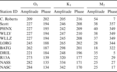
Results are included in Table VI for the three major constituents, and more complete tables are presented in the Supplemental Material. Discussion is deferred to a following section, except for one important topic that reflects on the use of GPS. Because of the particular orbit period of the GPS constellation, effects of orbit error and quasi-periodic multipath errors tend to be pronounced at K1 and its higher harmonics (King Reference King2006). Such errors, although fairly small in absolute terms, are probably occurring in our tidal estimates. For example, the two stations WLLY and WLLZ, being nearly collocated, should produce nearly identical tidal constants. Table VI shows identical estimates for O1 and almost identical estimates for M2, but not for K1 (although the differences are small: 2 mm in amplitude and 2° in phase). The K2 results also differ (Tables SIII & SIV). Moreover, at several stations, we find anomalously large amplitudes at higher harmonics (e.g. 5 and 7 mm in K4 at WLLY and LORG, and even 13 mm in K6 at LORG), where the likelihood of real compound tides existing at these frequencies is low (e.g. there are no comparable harmonics of O1 present). These possible errors in K1 and its harmonics, while relatively small, should be kept in mind in any future applications.
Major estimated tidal constants.

Amplitudes in mm; Greenwich phase lags in degrees.
Uncertainties (not tabulated) are much larger for the three last stations. More comprehensive tables with uncertainty estimates and greater precision are given in the Supplemental Material.
Finally, a point worth noting is that, in 1974, 29 days of tidal gravity measurements were collected at station C13 (see Fig. 1), ~28 km from GPS station BATG. Williams & Robinson (Reference Williams and Robinson1980) reported tidal constants deduced from these measurements. They found for O1, K1 and M2 the following amplitudes and phases: (34 cm, 190°), (30 cm, 200°) and (3 cm, 300°), respectively. Comparison with Table VI shows reasonable agreement with BATG, except for the amplitude of O1, where we find 26.2 cm, which is a large 8 cm discrepancy. Moreover, the gravity result giving an amplitude of O1 that is 4 cm greater than K1 is suspicious. Only at Cape Roberts do we find O1 exceeding K1 in amplitude, and there by only 4 mm. As the other amplitudes and phases are in reasonable agreement, one wonders whether the Williams & Robinson (Reference Williams and Robinson1980) O1 amplitude is a typographical error, but the same value occurs in the thesis of Williams (Reference Williams1979). Note that these gravity data have been assimilated into a number of global and regional tidal models, possibly leading to follow-on errors.
Tides at station DRIL
The GPS receiver at station DRIL was operational for three years, from late 2010 to late 2013. It is not included in the University of Nevada database (which actually has a different station DRIL, located in Australia). We have therefore here computed our own high-rate position solutions. The process we have used is similar to that employed by Blewitt et al. (Reference Blewitt, Hammond and Kreemer2018) mentioned above.
In the resulting elevation time series, an anomalous jump of ~1 m occurred on 15 November 2011. We suspect the antenna was raised at that time to avoid being snowed under. We adjusted data after this date downwards by 103 cm. In the three years during which the station was operational, it moved horizontally by a total of 2.31 km. This is farther than any of our other stations moved, owing to a combination of longer record length and high mean ice speed (see Table III). The station also experienced an elevation trend of -67.5 cm yr-1 over the three years. As with the other stations, this trend was removed before harmonic analysis.
Harmonic constants for station DRIL are included in Table VI and the more extensive Table SVIII.
Tides at three MacAyeal-Brunt-King stations
The three easternmost stations shown in Fig. 1 provide the only in situ tide observations in that sector of the ice shelf. They are, however, very limited because the time series are quite short (23 days or less). The stations were deployed by Brunt et al. (Reference Brunt, King, Fricker and MacAyeal2010) primarily to study the horizontal motion of the ice shelf and to compare this with similar horizontal measurements made in the Siple Coast ice streams > 600 km away. The two neighbouring stations, NASS and NASC, are separated by a large ice rift, which Brunt et al. (Reference Brunt, King, Fricker and MacAyeal2010) found induces differences in their horizontal motions, although one expects little difference in their vertical tides. The GPS data for the three sites are described by MacAyeal et al. (Reference MacAyeal, Brunt and King2008) and are available from the US Antarctic Program Data Center. The sampling rate is 15 s, although with many small gaps. Because spectral analysis is used in some aspects of our analysis, the time series have been resampled to hourly, without gaps.
Special methods are needed to extract tides from such short time series. We had initially planned to use a response analysis relative to the observed tide at either Cape Roberts or Scott Base, following the methods laid out by Cartwright et al. (Reference Cartwright, Munk and Zetler1969). However, the admittance curves at both gauges are so smooth, especially in the dominant diurnal band (Fig. 5), that estimation of tidal responses relative to the astronomical potential cannot yield very different results, and analysis relative to the potential is simpler to compute. We have therefore employed a standard response analysis (Munk & Cartwright Reference Munk and Cartwright1966), supplemented with a few individual higher-order harmonics (K4, etc.).
Results are included in Table VI & Tables SIX–SXI. The amplitudes of diurnal constituents are larger and the semidiurnal constituents smaller (with the exception of BATG) than all of the other stations discussed above. The three constituents included in Table VI are reasonably consistent among themselves after accounting for the much larger standard errors (~10 mm; see Tables SIX–SXI). The exception is K1, for which the solutions are in poorer agreement than formal error estimates might suggest, again probably owing to the problems of extracting K1 from GPS data. The phases of M2 appear at first glance discordant, but with standard errors of 10 mm and amplitudes of only 22–25 mm, the phases are in fact consistent within uncertainties.
Discussion
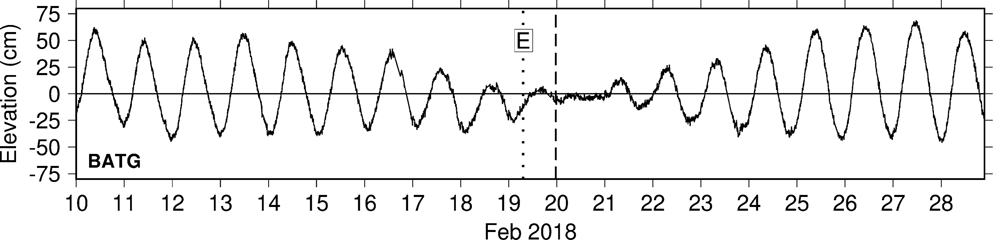
It has long been known that the tides near and under the Ross Ice Shelf are primarily diurnal, with all semidiurnal constituents being very small. Except for the three stations in the east, the amplitudes of K1 and O1 are comparable, within ~10%, and they are nearly identical at Cape Roberts. This leads to the unusual situation of the tide almost completely disappearing for a day or two each fortnight, as the two constituents come in and out of phase. (The cancellation is less complete near the winter or summer solstice; then P1 and K1, separated by 2 cpy, combine to outweigh O1.) A good example of the cancellation is shown in Fig. 9, where the observed tide at BATG essentially disappeared on 20 February 2018. The time of near-zero tide is slightly behind the time at which the diurnal astronomical forcing is at a minimum. This delay is analogous to the ‘age’ of the semidiurnal tide, generally attributed to tidal friction (Garrett & Munk Reference Garrett and Munk1971).
Observed tidal elevations at station BATG during part of February 2018, showing the nearly complete disappearance of the tide on the 20 February 2018. Symbol E marks the instant when the moon crossed the earth's equator, at which time the astronomical forcing of the lunar diurnal tide vanished (the solar diurnal tide reached zero in the next month during the equinox). The dashed line marks the time when the full diurnal potential reached a local minimum. The short delay between minimum forcing and zero observed tide is attributable, at least in part, to tidal friction, analogous to the ‘age’ of the semidiurnal tide (Garrett & Munk Reference Garrett and Munk1971).

The unusually small amplitudes of M2 seen at all examined stations reflect the wider-scale regional nature of M2, which is small across much of the south-east Pacific extending to the Antarctic coastline (see global charts in, for example, Lyard et al. Reference Lyard, Lefevre, Letellier and Francis2006). Moreover, within the Ross Sea itself is an M2 amphidrome, thought to be situated near the middle of the ice shelf in the vicinity of the dateline (MacAyeal Reference MacAyeal1984, Robertson Reference Robertson2005). The tide propagates clockwise around this amphidrome, and the constants of Table VI are consistent with that fact. From the south, the tidal wave first passes BATG, which, being closest to the amphidrome, has the smallest amplitude of all our stations. The wave then passes LORG, then DRIL and then swings around past the three eastern stations R13A, NASS and NASC. Another branch travels with a small delay westwards from LORG towards McMurdo Sound, and there is another small delay of ~17 min between the three close GPS stations WLLY, WLLZ and PHNX and Scott Base.
While the gross aspects of M2 have been known for some time (e.g. MacAyeal Reference MacAyeal1984), the seasonal perturbations in M2 are not so well known, even though they were first pointed out over a century ago (Darwin Reference Darwin and Darwin1907). In our analyses of the multi-year time series, we have routinely solved for seasonal sidelines of both M2 and O1 constituents; these are occasionally dubbed MA2, MB2 and OA1, OB1, respectively (note that OB1 coincides with a possible compound tide, MS1, which potentially confuses matters). Seasonal variations in the other major diurnal constituent, K1, cannot be so easily determined, as the frequencies of the two potential sidelines are already occupied by constituents S1 and ψ1, and these have both gravitational and radiational components that cannot be disentangled from K1 seasonality. For M2 and O1, we can here confirm what Darwin (Reference Darwin and Darwin1907) found: that M2 has a significant seasonal cycle in this region of the Antarctic, but that O1 has very little, in both relative and absolute terms. For example, at station PHNX, the amplitudes of OA1 and MA1 are 0.3 and 2.9 mm, respectively. At Scott Base, they are 1.1 and 2.3 mm, respectively.
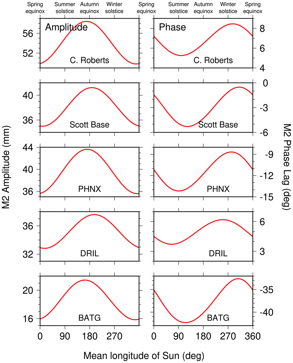
By simple trigonometry, the three constituents M2, MA2 and MB2 can be combined to form a single annually varying M2 pseudo-constituent. The resulting time-varying amplitudes and phases for five locations are shown in Fig. 10. At all locations, the M2 wave is seen to be suppressed in amplitude and retarded in time during Antarctica's late summer and autumn.
Seasonal variations of the M2 tide in amplitudes (left panels) and phase lags (right panels) for two tide-gauge stations and three GPS stations. Abscissa is h, the mean longitude of the sun, reckoned from the vernal equinox. Seasons at the top are boreal, not austral. Thus, M2 amplitudes peak during Antarctic winter and spring and are suppressed during Antarctic summer and autumn. These curves were obtained by combining the estimated M2, MA2 and MB2 constituents at each station into a single time-varying tidal amplitude and phase.

There are obvious questions that arise from these results, such as what seasonally varying dynamical mechanism is at work and why M2 is suppressed when the ice cover has melted. Seasonal modulations in tidal amplitudes and/or phases can arise in several ways. Changes in ocean stratification are capable of modifying barotropic transports and thus elevations by mechanisms associated with a time-varying eddy viscosity (Müller Reference Müller2012), as well as by modifying barotropic-to-baroclinic energy conversion (e.g. Mitchum & Chiswell Reference Mitchum and Chiswell2000). In polar regions, as here, seasonal variations in ice cover modify frictional dissipation by augmenting bottom drag with an ice-ocean drag (St-Laurent et al. Reference St-Laurent, Saucier and Dumais2008). There may well be feedback between ice cover and ocean stratification, as reduced ice cover leads to increased wind-driven mixing and increased heat exchange with the atmosphere (Venables & Meredith Reference Venables and Meredith2014). Our results show M2 being more strongly perturbed than the larger O1, which is probably related to the weakness of M2 currents and their subsequent greater sensitivity to environmental changes and to the different tidal dynamics acting in the two frequency bands (Robertson Reference Robertson2005). These are interesting dynamical questions, but they must be left to future modelling studies.
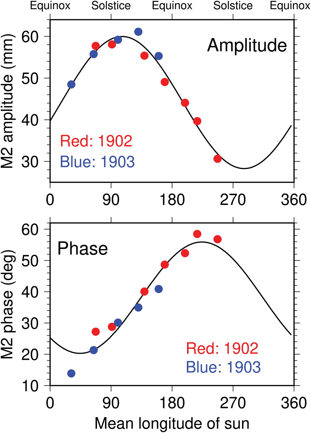
Reduced amplitudes and retarded phases in late summer and autumn, as seen in Fig. 10, are roughly consistent with Darwin's conclusions from the Discovery measurements, although he found peak amplitudes and phases occurring ~2 months earlier than ours (see Fig. 11, where Darwin's units and local phase convention have been converted to be consistent with Fig. 10). But note that the magnitudes of his observed modulations are much larger than ours. Whereas our amplitude modulations in Fig. 10 are approximately ±10%, Darwin's are closer to ±30%. Our phase modulations near Scott Base are no more than ±2°, while Darwin's are almost ten times that. Figure 3 does show modulations for some years that are much larger than average, but still much smaller than Darwin's.
Seasonal variations of the M2 tide, as deduced by Darwin (Reference Darwin and Darwin1907) from measurements made by the crew of the Discovery Antarctic expedition, converted to units and phase conventions consistent with Fig. 10. Each dot represents an independent estimate from 1 month of observations; red during 1902 and blue during 1903 show good consistency between the two years. No observations were taken during the Antarctic summer. Black curves are least-squares sinusoidal fits to Darwin's data. The modulations are much larger than those obtained from modern data, as depicted in Fig. 10.

We can offer two possible explanations for this disparity. 1) Some part of the Discovery crew's instrumental arrangement caused it to amplify and delay the tidal signal systematically, and apparently seasonally. Perhaps the ship had responded to the tide in some manner that was unaccounted for. One might envision the ship listing differently depending on the degree to which it was frozen in by ice, and this could have affected recorded amplitudes; it is more difficult to see how tidal phases could have been corrupted. 2) Alternatively, and more interestingly, it is possible that climate changes since 1902 have truly caused a change in the seasonal modulation of the tide. It is certainly conceivable that sea-ice cover or ocean stratification or both have substantially changed since 1902. Any investigation of this, of course, must begin by first understanding present-day seasonal changes. Explanation 1) is perhaps the more judicious and prudent to accept, but it has one serious drawback: Darwin, like us, reported no significant seasonal modulation in the much larger O1 constituent. While real environmental change could produce distinct tidal responses in the semidiurnal or diurnal frequency bands, it is difficult to envision any instrumental error capable of seasonally amplifying and delaying the small semidiurnal tide but not the larger diurnal signal. This adds weight to Explanation 2).
Summary
We have analysed the tidal motions of nine GPS stations situated on the Ross Ice Shelf. These data should help constrain and test future tide modelling work. The GPS-derived tide estimates complement and extend the high-quality observations from the tide gauges at Scott Base and Cape Roberts. The latter reveal, however, shortcomings in any tidal time series shorter than 10 years or so. For example, N2 determined from only a couple years of data (Goring & Pyne Reference Goring and Pyne2003) will be in error by > 10% owing to the presence of a significant 3N2 constituent, arising from third-degree terms in the moon's astronomical potential. The diurnal tides M1 and J1 are similarly affected by the third-degree potential (Fig. 6).
The remarkable tide measurements made through the winter Antarctic ice during the Discovery expedition (Darwin Reference Darwin and Darwin1907) established the basic tidal facts of the Ross Sea: dominant diurnal tides and an unusually small M2, the latter with seasonal perturbations in both amplitude and phase. The M2 perturbations reported by Darwin were either systematically too large or else, more intriguingly, they open a possible window to climate changes across 120 years; at this point, we cannot say which is the case. Understandably, the Discovery measurements, obtained during harsh conditions, were not of a quality one normally obtains at a standard tide gauge, but Darwin found that they were of ‘sufficient accuracy to obtain an insight into the nature of the Antarctic tides’, which is certainly true. Nonetheless, he cautioned, ‘it would not be possible to make a very good tide-table from the constants, but no one wants a tide-table for Ross Island’ (Darwin Reference Darwin and Darwin1907, p. 382). We may forgive Darwin for failing to anticipate the stringent tide-prediction accuracies now needed for modern satellite missions, and for other oceanographic and geodetic applications, even in the remote Ross Sea.
Supplemental material
Eleven supplemental tables will be found at https://doi.org/10.1017/S0954102020000498
Acknowledgements
A portion of the work was performed at the Jet Propulsion Laboratory, California Institute of Technology, under contract with NASA. Sea-level data for Cape Roberts are available from Land Information New Zealand (LINZ, https://www.linz.govt.nz). We thank Glen Rowe of LINZ for sending hourly data and for notes about data quality. Modern data at Scott Base were obtained from the University of Hawaii Sea Level Center (https://uhslc.soest.hawaii.edu). The Nevada GPS data are available at http://geodesy.unr.edu. The raw GPS data are provided by the GAGE Facility, operated by UNAVCO, Inc., with support from the National Science Foundation and NASA under NSF Cooperative Agreement EAR-1724794. We thank Thomas Nylen for information about the GPS sites. We thank Laurie Padman for helpful comments on the paper. The first author is indebted to the late George Platzman for (among many other things) his copy of the collected papers of Sir George Darwin, which include Darwin's Reference Darwin and Darwin1907 study of the Discovery measurements.
Author contributions
KML began the study and compiled initial GPS solutions. BJH computed some of the GPS solutions. RDR undertook all tidal analyses and wrote the bulk of the paper with input from others.
Financial support
This work was supported by the National Aeronautics and Space Administration through the OSTST and SWOT projects.