

1. Introduction
The streaky structure characterized as streamwise filaments of low-speed fluid is ubiquitous in wall-bounded turbulent flows, and has been studied for more than five decades since the initial observation by Kline et al. (Reference Kline, Reynolds, Schraub and Runstadler1967). As one of the most significant coherent structures in both transitional and turbulent boundary layers, a low-speed streak (LSS) is highly relevant to the bursting process and turbulence production. There are differing interpretations of LSSs, from their formation mechanism to streak instability, and their role in transition and turbulence. The prevailing hairpin-like interpretations ascribe the formation of LSSs to the lift-up effect caused by hairpin-like structures. By systematic investigation of near-wall turbulent flow, Kline et al. (Reference Kline, Reynolds, Schraub and Runstadler1967) and Kim, Kline & Reynolds (Reference Kim, Kline and Reynolds1971) identified and characterized LSS and turbulent bursting behaviour. The mechanism for streak formation that they proposed was based on stretched and lifted vortex elements. Head & Bandyopadhyay (Reference Head and Bandyopadhyay1981), based on observations of laser-illuminated smoke visualizations, proposed that individual streaks are the result of an upflow between the legs of lifted hairpin vortices. Based on extensive experimental work, Smith & Metzler (Reference Smith and Metzler1983), Smith (Reference Smith1984) and Smith et al. (Reference Smith, Walker, Haidari and Sobrun1991) hypothesized a model of LSSs and bursting behaviour which suggests that the elongated LSSs, spaced at  ${\rm \Delta} \lambda ^+ \approx 100$, are lower-speed regions of upwelling flow induced by the legs of a sequence of lifting hairpins. Jiménez & Moin (Reference Jiménez and Moin1991) studied the structures and dynamics of turbulence in the near-wall region using a minimal channel flow, and observed very long intermittency cycles that were closely related to near-wall streaks. Jiménez & Pinelli (Reference Jiménez and Pinelli1999) further proposed that an autonomous turbulence regeneration cycle exists in the near-wall region, involving quasi-streamwise vortices and longitudinal velocity streaks. In contrast to previous research that mainly focused on the near-wall region of turbulent boundary layers, Adrian, Meinhart & Tomkins (Reference Adrian, Meinhart and Tomkins2000) performed a quantitative experiment at higher Reynolds number by applying particle image velocimetry (PIV) primarily to the outer region of a turbulent boundary layer. Based on their results, they argued that LSSs are part of uniform momentum zones created by induction of the hairpin packets.
However, there is no clear consensus on the origin of the vortices. Waleffe (Reference Waleffe1997) proposed a self-sustaining process (SSP) to explain the turbulence regeneration process. The SSP consists of three phases: (1) formation of streaks by streamwise vortical rolls, (2) streak instability and (3) nonlinear feedback to the rolls. He emphasized that what drives the SSP is the instability of the streaks. Schoppa & Hussain (Reference Schoppa and Hussain2002) used direct numerical simulation (DNS) to study the relationship between structure generation and streak instability, and determined that near-wall streamwise vortices sometimes arise from the instability of LSSs. They stressed that the streak transient growth mechanism is more important for streak breakdown and vortex generation. A mechanism for inner–outer region cross-talk, suggested by Marusic, Mathis & Hutchins (Reference Marusic, Mathis and Hutchins2010), and later verified by experiment, is that large-scale motions (LSMs) and very large-scale motions (VLSMs) appear to organize the SSP cycle (Naka et al. Reference Naka, Stanislas, Foucaut, Coudert, Laval and Obi2015).
LSSs are not always the result of vortical structures. It is known that LSSs disappear if the  $v\,\partial U/\partial y$ term is removed from the governing equation, where
 $U$ is the averaged streamwise velocity and
 $v$ is the wall-normal velocity fluctuation (Hama Reference Hama1962; Kim & Lim Reference Kim and Lim2000; Chernyshenko & Baig Reference Chernyshenko and Baig2005). Therefore, the streaky structure in a turbulent shear layer must be dependent on the wall-normal fluctuation velocity. A linear inviscid model was proposed by Landahl (Reference Landahl1980, Reference Landahl1990), who hypothesized that LSSs will develop from any initial, local three-dimensional (3-D) disturbance with non-zero net vertical momentum. Such disturbances could be initiated from a local region of inflectional instability with spanwise asymmetry, such as the case of an oblique wave disturbance. Chernyshenko & Baig (Reference Chernyshenko and Baig2005) proposed that LSSs form from the combined action of (1) a lift-up of wall-region fluid, (2) amplification within the mean shear and (3) viscous diffusion, without the need of hairpin vortices. Hama & Nutant (Reference Hama and Nutant1963) proposed that an amplified perturbation wave in the wall shear layer (termed a kink) has a strong tendency to form 3-D vortex loops. The kink structure was found to be a 3-D wave packet, called a soliton-like coherent structure (SCS) (Lee Reference Lee1998, Reference Lee2000; Lee & Li Reference Lee and Li2007), which spans the whole boundary layer from the near-wall region to the edge of the boundary layer. LSSs in the transitional boundary layer were observed to consist of several SCSs (Lee & Wu Reference Lee and Wu2008; Jiang et al. Reference Jiang, Lee, Chen, Smith and Linden2020). Hairpin vortices were hypothesized to develop from the edges of a SCS, as the SCS moves away from the wall.
The similarity between late-stage transition and developed turbulence has been examined in several investigations. The experiments by Nishioka, Asai & Iida (Reference Nishioka, Asai and Iida1981) and Nishioka & Asai (Reference Nishioka and Asai1984) may have been the first to show a close similarity between the near-wall structure/activity in the late stage of the transition (K-regime breakdown) and the near-wall coherent structure/motion in wall turbulence. The evolution from a local high-shear layer to the appearance of discrete vortices was presented quantitatively. In their papers, the occurrence of hairpin vortices was explained from the high-frequency secondary instability. The finding that a hairpin is a manifestation of a secondary instability due to a pre-existing distortion of the boundary layer is also supported by a recent investigation of Hack & Moin (Reference Hack and Moin2018), who further propose that the patch of low-momentum fluid (LSSs) at the centre of the hairpin is not primarily an outcome of the hairpin itself, although the latter may contribute to it. Sayadi, Hamman & Moin (Reference Sayadi, Hamman and Moin2013) evaluated the breakdown of K- and N-regimes to turbulence during late-stage transition using DNS, and they determined that the flow statistics and near-wall dynamics are similar to a turbulent boundary layer. Based on that observation, they proposed late-stage transition, manifested by hairpin packets, as a reduced-order model of a turbulent boundary layer.
The collective simulation and experimental studies reached no consensus on the near-wall turbulence production cycle regarding the types of flow structures, and their development, hierarchy and symbiosis. LSSs, hairpin vortices, the so-called ‘bursts’ and the interdependence of these structures/events are subject to a number of different interpretations. Some of these disparate interpretations arise from the limitation of experimental techniques that rely on qualitative visualization, or restrictive two-dimensional (2-D) measurements localized in space and time. Other issues arise from the flaws in post-processing methods, such as isosurface methods or frame-dependent Eulerian criterion for structure detection.
The present investigation attempts to establish the essential skeleton of the LSSs by using a combination of both qualitative and quantitative techniques to assess and compare the flow structure of a turbulent boundary layer. In contrast to previous 3-D PIV experiments applied to fully developed turbulent boundary layers at relative high Reynolds number (Schröder et al. Reference Schröder, Geisler, Elsinga, Scarano and Dierksheide2008; Dennis & Nickels Reference Dennis and Nickels2011; Gao, Ortiz-Dueñas & Longmire Reference Gao, Ortiz-Dueñas and Longmire2013), the present study focuses on early turbulent flow at low Reynolds number, in order to illustrate the early origin and metamorphosis of turbulent flow structure. Lagrangian tracing methods are applied to time-resolved 3-D data obtained from tomographic particle image velocimetry (tomo-PIV), illustrating the spatiotemporal evolution of LSSs, as well as details of the bursting process. This is done using a process of Lagrangian-averaged vorticity deviation to detect vortices within the datasets. The evolution of Lagrangian-detected coherent structures and streak–vortex interaction is also illustrated, which has not been effectively addressed in previous studies. Based on the data analysis, detailed comparisons and synthesis are carried out to establish the apparent flow structure present and its symbiosis, leading to hypothesized mechanisms for the streak formation process, the bursting process and the generation of hairpin vortices.
2. Experiment set-up and data processing
2.1. Experimental techniques
The experiments were performed in the Peking University Water Tunnel (PWT), which is an open-surface recirculating water channel with a cross-section of  $0.4\ \textrm {m}\times 0.4\ \textrm {m}$ and length of 6 m. The tunnel free-stream velocity range is from 0.1 to 1.3 m s
 $^{-1}$, with a turbulence level of
 $0.77\,\%$ for tunnel velocities of 0.1–0.3 m s
 $^{-1}$. The plate has a chord length of 1.8 m, a span of 0.8 m and a thickness of 15 mm, as shown in figure 1(a) and (b) for side view and plan view, respectively. The flat plate was mounted vertically on the centreline of the tunnel at zero angle of attack. An adjustable flap mounted at the trailing edge of the plate was employed to force an early transition to turbulence at
 $x\approx 400$ mm.
Experimental set-up of tomo-PIV: (a) side view of set-up for hydrogen bubble visualization; (b) plan view of set-up for hydrogen bubble visualization; (c) schematic view of horizontal wire; (d) schematic view of vertical wire; (e) schematic layout of the arrangement of the tomo-PIV system; and (f) a picture showing the camera configuration.

The present study was done using both qualitative hydrogen bubble flow visualization, and selective, detailed tomo-PIV studies. Since hydrogen bubble visualization was the method employed for the initial identification of LSSs, the present hydrogen bubble studies were done to provide comparative time-line studies of the near-wall behaviour of the low-Reynolds-number turbulent boundary layer, to assure that the flow structure was comparable to prior studies (Kline et al. Reference Kline, Reynolds, Schraub and Runstadler1967; Kim et al. Reference Kim, Kline and Reynolds1971; Smith Reference Smith1984). A series of hydrogen bubble time-line visualizations were done employing both horizontal-wire and vertical-wire configurations, as described by Lee & Li (Reference Lee and Li2007) and Sabatino et al. (Reference Sabatino, Praisner, Seal and Smith2012); see figure 1(c) and (d). The hydrogen bubble wire was 0.03 mm diameter platinum wire. For plan-view visualization, a horizontal wire is kept taunt by a weight hung on the opposite side of the working surface. The distance of the wire from the plate surface was adjusted using insulated spacers beneath the wire (figure 1c). For side-view visualizations, a vertical wire was configured using a probe support employing a non-conductive fibre (human hair); the vertical bubble wire was tied around the centre of the fibre, placed in moderate tension, and soldered to the upper wire support (figure 1d). A portion of wire was left extending below the fibre to show near-wall flow behaviour. By pulsing the current through the hydrogen bubble wire at a constant frequency, a pattern of time-lines is created, as shown in figure 1(c,d).
These hydrogen bubble visualization studies were used to confirm the qualitative near-wall flow structure and guide the measurements using tomo-PIV, focusing on the near-wall region where LSSs develop. The free-stream velocity employed for both the hydrogen bubble and tomo-PIV was approximately 0.17 m s $^{-1}$, and the distance,
 $x_d$, from the leading edge to the centre of the measurement region was 502 mm. The tomo-PIV configuration is shown in figure 1(e) and (f). Four high-speed complementary metal oxide semiconductor (CMOS) cameras (Photron FASTCAM SA4) with resolution of
 $1024\times 1024$ pixels at frame rates up to 3600 frames per second were used, in a cross-configuration arrangement. The cameras are fitted with Nikon lenses of 200 mm focal length, with aperture of
 $f$/11. Illumination was provided by a high-speed laser generator from Beijing ZK Laser, DCQ-30Q, a single-cavity double-pulse laser system emitting a beam of wavelength 527 nm (30 mJ at 1 kHz). The four cameras and laser system were synchronized using a LaVision's PTU timing controller. The thickness of light volume generated by the optical lenses and the mirror was nearly 310 viscous units within the regions of interest, illuminating tracers of hollow glass particles from Potter Industries. The particles of mean diameter 11
 $\mathrm {\mu }$m were introduced into the water tunnel 6 m downstream of the test section to assure that the particles were fully mixed and uniformly distributed after circulating to the measurement site. Experiments were conducted at a particle image density of 0.098 particles per pixel, which corresponds to particle concentrations of approximately 2.3 particles mm
 $^{-3}$.
The tomo-PIV sampling frequency was 500 Hz, i.e. the time increments  ${\rm \Delta} t^+\approx 0.42$ viscous time units. All cameras were carefully adjusted in the Scheimpflug condition, i.e. applying the Scheimpflug condition between the image plane, lens plane and subject plane assures that the final residual calibration errors for all cameras was less than 0.1 pixels. The digital resolution was 13.37 pixels mm
 $^{-1}$ for the calibration field of view. The measurement domain extended 815 viscous length units in both the streamwise and spanwise directions. Before the reconstruction process, image pre-processing with a Gaussian smoothing filter (
 $3 \times 3$ pixels) was applied on the raw particle images. Volume self-calibration (Wieneke Reference Wieneke2008) was used on the pre-processed particle images. Volume reconstruction was achieved by sequential motion tracking enhancement (SMTE; Lynch & Scarano Reference Lynch and Scarano2015). The reconstructed volume was
 $1041 \times 1048 \times 187$ voxels. A multi-pass approach of four steps was carried out for the volume correlation, and the interrogation volume size for the final pass was
 $16 \times 16 \times 16$ voxels (corresponding to spatial resolution of
 $12.52 \times 12.52 \times 12.52$ wall units) with a 75 % overlap, yielding 0.3 mm grid spacing (3.13 wall units). As a final step, a Gaussian smoothing filter of
 $3 \times 3 \times 3$ vectors was applied to the velocity data.
Proper orthogonal decomposition (POD) analysis is effective for noise removal and extraction of the higher modes in turbulent flow (Moin & Moser Reference Moin and Moser1989). In the present paper, POD analysis was applied to the smoothed velocity datasets, and the first four leading-order POD modes are extracted. As an additional note, the details of POD filtering and its low-order representation are discussed in appendix A.
2.2. Properties of the boundary layers and PIV accuracy
The mean turbulent boundary layer velocity profile obtained from the tomo-PIV datasets is shown in figure 2(a), in comparison with fitted curves of Musker (Reference Musker1979) and Spalding (Reference Spalding1961). In figure 2,  $y^+$ is the wall-normal coordinate scaled on the turbulent length scale
 $l=\nu /u_\tau$, such that
 $y^+=u_\tau y/\nu$, and
 $U^+$ is the scaled velocity with
 $u_\tau$, such that
 $U^+=U/u_\tau$. The profile agrees well with fitting curves using the models of Musker (Reference Musker1979) and Spalding (Reference Spalding1961). The root-mean-square (r.m.s.) streamwise and spanwise velocities are scaled with
 $u_\tau$ and plotted against
 $y^+$ in figure 2(b). The data agree well with the DNS data of Wu & Moin (Reference Wu and Moin2009) at
 $Re_\theta = 900$ and Spalart (Reference Spalart1988) at
 $Re_\theta = 670$. However, it is apparent that the r.m.s. velocity is slightly underestimated. A comparison to the experimental
 $u'_{rms}$ data of Purtell et al. (Reference Purtell, Klebanoff and Buckley1981) at
 $Re_\theta = 465$ shows that the present results are relatively larger. These comparisons suggest that
 $Re_\theta$ for the present experiment is expected to be between 465 and 670.
(a) Turbulent boundary layer mean velocity profile plotted in log–linear coordinates, with  $\kappa = 0.41$ and
 $B = 5.0$. The fitting curves use the models of Musker (Reference Musker1979) and Spalding (Reference Spalding1961). (b) Root-mean-square streamwise and spanwise velocity profile comparison: pluses, present PIV results; circles, Wu & Moin (Reference Wu and Moin2009) at
 $Re_\theta = 900$; triangles, Spalart (Reference Spalart1988) at
 $Re_\theta = 670$; stars, Purtell, Klebanoff & Buckley (Reference Purtell, Klebanoff and Buckley1981) at
 $Re_\theta = 465$; dashed lines, velocity approximation based on the first four POD modes; red,
 $u'_{rms}$; blue,
 $w'_{rms}$.

The position of the wall is usually an important source of uncertainty (Titchener, Colliss & Babinsky Reference Titchener, Colliss and Babinsky2015). The wall deviation  ${\rm \Delta} h$, defined as the difference of nominal wall position
 $y_0^\prime$ and real wall position
 $y_0$, is considered in this study. By using a gradient descent algorithm, which is an iterative optimization procedure updating parameters based on the gradient of the objective function (Shalev-Shwartz & Ben-David Reference Shalev-Shwartz and Ben-David2014), both friction velocity and wall deviation are obtained. The final result gives
 $u_\tau = 0.0104$ m s
 $^{-1}$ and
 ${\rm \Delta} h = -0.38$ mm. Thus, all the wall-normal coordinates are corrected as
 $y=y^\prime -{\rm \Delta} h$. The other source of uncertainty is the experimental error from the non-uniformity of the laser light. The thickness of the laser volume (i.e. the vertical height of the data window) is
 $10 < y^+ < 150$, which is the region of interest in this study. This data window contains part of the buffer layer and the log-law region of a turbulent boundary layer. The light volume is parallel to the flat plate, which means that the spatial resolution may decrease slightly in the region of
 $y^+>100$ due to a weaker light intensity at the edge of the laser volume. The calibration inaccuracies were reduced to less than 0.01 pixels (0.08 wall units) by applying volume self-calibration on the pre-processed images. The reconstruction accuracy of the tomo-PIV was determined by the reconstruction signal-to-noise ratio (SNR), defined as the intensity level encountered in the reconstructed region compared with that outside the illumination region. The condition
 $SNR \geq 2$ is considered as the lower limit identifying a tomographic experiment with good reconstruction quality (Scarano Reference Scarano2013). The distribution of light intensity across the depth of the measurement volume was determined using a MART tomographic algorithm, which gave
 $SNR> 2.17$, which was considered an acceptable reconstruction level.
3. Experimental results
3.1. Flow visualization
3.1.1. Hydrogen bubble visualization
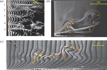
Examples of hydrogen bubble time-line images for a turbulent boundary layer, both a plan view and two side views, are shown in figure 3. Figure 3(a) is a time-line image showing five LSSs (labelled 1 to 5) with the hydrogen bubble wire at  $y^+ = 20$. The average spacing of neighbouring LSSs is
 $\lambda ^+ = 97$, which is in accord with Smith & Metzler (Reference Smith and Metzler1983). The side-view image in figure 3(b) reveals the presence of a streamwise vortex (labelled B), and also a strong inflectional pattern in the outer region (labelled A). It was observed that a streamwise vortex is initiated by the breakdown of a local instability, which is closely related to the combined processes of ejections and sweeps. Different structures are observed to develop during this breakdown process, depending on the relative strength of the ejection and sweep. When the ejection is weak, the development of the ejection into a burst occurs only in the near-wall region. If a strong sweep develops, a streamwise vortex may be generated such as B in figure 3(b). When the ejection from the wall is strong enough, the low-momentum wall fluid may be ejected into the outer region, which results in the development of a strong, hump-like inflectional region, like the pattern labelled A in figure 3(b). If the downward sweep is sufficiently strong, a rotational pattern with transverse orientation will develop, as reflected by the apparent roll-up of H1 and H2 in figure 3(c), associated with the ejections (E) and sweeps (S). This inflow can also produce an incipient streamwise vortex near the wall, as labelled L in figure 3. These patterns, like L, are observed to develop into streamwise vortices similar to that identified as B in figure 3(b), with their sense of rotation around the red dotted line shown on figure 3(c).
Hydrogen bubble visualization of turbulent boundary layers: (a) plan-view time-lines at  $y^+=20$; and (b,c) side-view time-lines. The yellow bars on the images indicate the physical scales in viscous lengths
 $\nu /u_\tau$. E, ejection; S, downward sweep; R, rotation. The flow is from left to right.

When they are compared, the images of figure 3 are in accord with similar images of Kim et al. (Reference Kim, Kline and Reynolds1971), Smith (Reference Smith1984) and Lu & Smith (Reference Lu and Smith1991), indicating that the low-Reynolds-number boundary layer of the present study does reflect the same type of flow structure and behaviour as observed in past visualization studies. A detailed review of the hydrogen bubble data appears to support the previous dynamical model suggested by Kim et al. (Reference Kim, Kline and Reynolds1971). In Kim's model, upward ejection of fluid from an LSS is perceived as the driving mechanism that results in the development of streamwise and spanwise vortices. It is our hypothesis that this breakdown and ejection of the LSS is initiated by the amplification of 3-D wave behaviour. In the following section, we will provide several types of time-line and material surface visualizations of the tomo-PIV results to examine this hypothesis, which links LSS breakdown, and subsequently the bursting process, to a process of 3-D wave development.
3.2. LSSs in ‘tomographic visualization’
‘Tomographic visualizations’ are time- and streak-line patterns extracted from the tomo-PIV database by applying Lagrangian tracking to the marked particles. The LSS time-line patterns for a turbulent boundary layer are similar to those observed for a transitional boundary layer, although they behave in a less stable manner. Figure 4 is a plan-view time-line visualization of two LSSs in the near wall of our turbulent boundary layer database. The generation line is located at  $x = -45$ mm (
 $x^+ = -446$) relative to the centre of measurement (the distance from the leading edge to the centre of measurement
 $x=0$ is 502 mm) and
 $y = 2.58$ mm (
 $y^+ = 27$). The frequency of time-line generation is 50 Hz, and the image shown is at
 $t^+ = 164$ after initiation of the time-line generation. The circular markers shown initiating at I and II represent the location of the two LSSs, reflected by the subsequent time-line deformation. The two streaks shown have a spacing of
 ${\rm \Delta} z^+ \approx 100$ (see the double-headed arrows in figure 4), which is essentially the same as shown in the hydrogen bubble visualization of figure 3(a). An analysis of the characteristics of, and the flow behaviour spawned by, the two LSSs I and II in figure 4 (LSS-I, LSS-II) will be the primary focus of the remainder of this paper.
A sequence of time-lines at  $t^+=164$, generated at 50 Hz and initiated at
 $y^+ = 27$, illustrating LSSs in a turbulent boundary layer. The markers trace the location of the centre of two LSSs, designated I and II.

Figure 5 is a series of plan and side views of time-line patterns for LSS-I, identified in figure 4, taken at times  $t^+ = 164$, 183 and 203. The plan-view time-lines, shown in figure 5(a–c), are initiated at
 $y^+ = 27$ at a frequency of 50 Hz. They reveal a transient flow structure passing across the domain of LSS-I. The convection speed
 $V_c$, which was determined by tracking the kink in the time-lines, is approximately
 $64\,\%$ of the free-stream velocity. Note that the plan-view time-line patterns in figure 5(b) and (c) appear to show the streak lifting away from the wall, and becoming convoluted laterally, suggesting that the streak is either moving upwards into some less-organized flow, or possibly undergoing some type of 3-D instability.
Plan-view and side-view time-line patterns showing the evolution of streak I from figure 4. (a–c) Plan views of horizontal time-lines initiated at  $y^+ = 27$ as they appear respectively at (a)
 $t^+=164$, (b)
 $t^+=183$ and (c)
 $t^+=203$. (d–f) Side views of vertical time-lines initiated at
 $z^+ = 32$ as they appear respectively at the same times (d)
 $t^+=164$, (e)
 $t^+=183$ and (f)
 $t^+=203$. The sequences of red dot markers superposed on the time-lines reflect streak-line behaviour for markers initiated at
 $y^+=27$ and 36.

In order to better understand the spatio-temporal evolution of LSS-I, patterns of vertical time-lines, synchronized with the plan views of figure 5(a–c), were generated using time-lines initiated at  $z^+ = -32$, essentially the centre of the passing streak I. These patterns are markedly similar to the vertical time-line patterns for a controlled transitional boundary layer (Wortmann Reference Wortmann1981), as well as the instantaneous velocity profile results for the near wall of a turbulent boundary layer shown in Lu & Smith (Reference Lu and Smith1991). The red dot markers in figure 5(d–f) indicate streak-line behaviour originating from both
 $y^+ = 27$ and 36. When compared to the plan-view patterns of figure 5(a–c), figure 5(d–f) indicates that, whereas the plan views reflect a strong LSS, the side-view patterns display an obvious inflectional region in the corresponding vertical profiles.
Figure 6 is a sequence of synchronized plan- and side-view time-line patterns for LSS-II identified in figure 4 at  $t^+ = 131$, 150 and 170 of the data sequence (relative to the initiation of the first time-line). The development of streak II, shown in figure 6(a–c) by plan-view time-lines generated at
 $y^+ = 27$, appears longer and laterally larger than that of streak I in figure 5(a–c).
Plan-view and side-view time-line patterns showing the evolution of streak II from figure 4. (a–c) Plan views of horizontal time-lines initiated at  $y^+ = 27$ as they appear respectively at (a)
 $t^+=131$, (b)
 $t^+=151$ and (c)
 $t^+=170$. The sequences of red dot markers in (a–c) correspond to streak-lines initiated at
 $z^+ = -59$. (d–f) Side views of vertical time-lines initiated at
 $z^+ = 59$ as they appear respectively at the same times (d)
 $t^+=131$, (e)
 $t^+=151$ and (f)
 $t^+=170$. The sequences of red dot markers in (d–f) are streak-lines initiated from
 $y^+=21$, 27 and 36.

Figure 6(a–c) shows that the time-lines which flank the low-speed region appear to temporally intersect and crimp (this is most obvious in figure 6c), which appears to indicate the presence or development of streamwise rotation. The vertical time-line patterns of figure 6(d–f), generated at  $z^+ = 59$ (the initial location of LSS-II detection), also behave somewhat differently than the vertical time-line patterns for LSS-I (figure 5d–f). This may reflect that LSS-I and LSS-II are in different stages of development. Notice that the kink region very near the wall, indicated by K in figure 6(f), is similar to the kink labelled K in the hydrogen bubble visualization of figure 3(b). The kink appears as a small arch moving away from the wall, which seems to be the same type of kinking behaviour as observed in the hydrogen bubble visualizations of Hama & Nutant (Reference Hama and Nutant1963).
The time-line patterns shown in figures 5 and 6 are different from the time-line patterns reconstructed from a flow field with a distinct vortex. See the examples shown in figures 28 and 29 in appendix B for a  $\Lambda$ vortex and a streamwise vortex, respectively. In the presence of a vortex, time-line patterns are characterized as folding and twining lines. But when there is only a high-shear layer, the time-lines tend to intersect and crimp, but do not appear as a vortex-shaped pattern, such as the time-lines shown in figure 28(a) for K-regime transition prior to the appearance of a
 $\Lambda$ vortex. When there is a wave structure in a flow field, 3-D time-lines appear as concentrations and dispersions, manifesting as a hump-like pattern without an intersection of time-lines. See the example of O-regime transition in figure 30. Thus, figures 5 and 6 indicate that the LSS is not a vortex structure, and high-shear layers develop at the sides of LSSs.
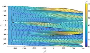
Figure 7 shows contours of wall-normal position superposed with the expanded time-line surface corresponding to figure 4. LSSs were identified by tracing the peak of the time-lines, as indicated by the white dashed lines on figure 7. The contours show that an LSS usually appears as a localized hump, accompanied by regions of depression, high-speed streaks (HSSs), flanking the side of the LSS. The interface between an LSS and an HSS is the location where high-shear layers develop. Note that the time-lines shown in figure 7 are 3-D, and thus the geometry of an LSS can be obtained from its position ( $P_x,P_y,P_z$). The streamwise length
 $l^+$ of an LSS is calculated as
 $(P1_x-P0_x)$, and the spanwise shift
 $s^+$ is obtained from
 $(P1_z-P0_z)$, where
 $P0$ and
 $P1$ are the start and end positions of an LSS, determined manually, as indicated on figure 7.
The wall-normal variation of LSSs at  $t^+ = 164$, extracted from the time-lines initiated at
 $y^+ = 27$ (corresponding to figure 4). The colour contours indicate the wall-normal position of the time-line surface. White dashed lines indicate identified LSSs.

Figure 8 shows the distribution of  $l$ and
 $s$ for 125 identified LSSs reconstructed from tomo-PIV data within a time interval of
 ${\rm \Delta} t^+ = 960$. The distribution shows that the length
 $l^+$ of an LSS varies from 150 to 700, with two dominant length scales at
 $l^+ \approx 300$ and 450. The former value is very close to the prediction from the linear stability analysis by Schoppa & Hussain (Reference Schoppa and Hussain2002) for typical streaks in wall turbulence and the most probable value for the streamwise wavelength of the secondary streak in experiments (Asai et al. Reference Asai, Konishi, Oizumi and Nishioka2007). The spanwise variation of
 $s$ reveals that LSSs are not completely streamwise, but lie within a range of
 $|s^+|<50$.
Histograms showing the distribution of 125 identified LSSs categorized according to their geometry: (a) streamwise length,  $l^+$; and (b) spanwise shift,
 $s^+$.

3.3. Spatio-temporal evolution of LSSs
It is difficult to determine the exact location of LSSs and their development without use of some quantitative assessment process. Using ‘tomographic visualization’, the spatio-temporal evolution of LSSs can be examined. The temporal evolution of LSS-II is shown in figure 9, which is a composite illustration of the temporal changes in the time-line patterns as LSS-II spatio-temporally evolves. The black lines trace the peak of LSS-II. The dotted line on figure 9 traces the temporal normal displacement of the peak of the streak pattern. In figure 9(a), spanwise time-line segments of width  $z^+ = 41$ are shown for progressively increasing times from
 $t^+= 111$ to 190. Each time-line segment is centred on the peak of the time-line patterns visualizing LSS-II: the progressive evolution of the streak pattern is shown left-to-right for the indicated
 $t^+$ times.
Temporal evolution of LSSs. (a) Temporal evolution of LSS-II (see figure 4) from  $t^+= 111$ to
 $190$; this shows the temporal variations in the time-line patterns of span
 $\textrm {d} z^+ = 41$ (using a compressed
 $z^+$ scale), encompassing the span of LSS-II. (b–e) Temporal evolution of four selected LSSs, tracing the temporal normal displacement of the peak of the streak pattern initiated at
 $y^+ = 27$, with time interval of
 $\textrm {d} t^+ = 8.74$. The changes in the time-line patterns are shown from left to right for increasing time as indicated by the dotted lines. W indicates a second 3-D amplification.

Figure 9(a) shows that the vertical extent of the streak increases slowly from  $t^+ = 111$ to
 $t^+ = 164$ (termed ‘early slow lifting stage’), but appears to begin a wave amplification process at
 $t^+ = 177$ (termed ‘sharply outward motion’), followed by an abrupt decrease in amplitude (termed ‘abruptly inward motion’). These processes of ‘streak lifting’ followed by ‘sharply outward motions’ are markedly similar to the previous observation of a bursting sequence (Kim et al. Reference Kim, Kline and Reynolds1971; Acarlar & Smith Reference Acarlar and Smith1987b; Haidari & Smith Reference Haidari and Smith1994). The undulation of LSS-II observed in figure 9 could also be interpreted as the behaviour of the streak as an amplified 3-D wave, which interacts with the higher-speed outer flow, becomes unstable, amplifies and subsequently rolls up into another flow structure (e.g. hairpin vortex). Note that figure 9(a) also shows the development of an incipient second 3-D structure, labelled W, which initiates at
 $t^+ = 164$, and appears to undergo a subsequent amplification process as time increases. Four selected streak developments obtained in a similar way as figure 9(a) are shown in figure 9(b–e). They reveal that LSSs travel downstream in a wave-like manner, lifting up from the near-wall region. The average streamwise advection speed of the streaks is 60 % of the free-stream velocity, and the average upward wave velocity is 3 % of the free-stream velocity.
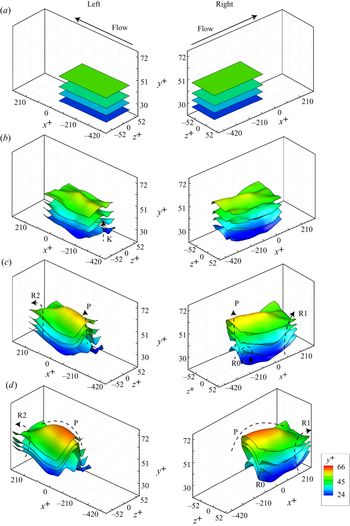
The wave-like undulation and oscillation of LSSs is further examined by applying Lagrangian tracing of several material surfaces initiated in the region of LSS-I, as shown in figure 10. These are flat material surfaces initially spanning  $0>x^+>-420$ by
 $52>z^+>-52$ that are allowed to evolve within the database flow field to illustrate the surface deformation in time–space. In order to illustrate the detail of the flow development, two different perspective views of the four developing material surfaces are shown in both the left and right columns of figure 10. The left column shows oblique views of the surfaces as viewed from their left side as they move with time in the positive
 $x$ direction; the right column shows oblique views of the same surfaces as viewed from their right side as they again move in the
 $x$ direction. The four initial material surfaces at
 $y^+ = 27$, 33, 39 and 49 are shown in figure 10(a). After a time increment of
 ${\rm \Delta} t^+=9$, figure 10(b) at
 $t^+ = 173$ shows a small wave-like structure labelled K forming near the trailing edge of the material sheets at approximately
 $z^+ = -30$. The LSS region revealed in the horizontal time-line patterns of figure 5(a) and the inflectional region appearing in the vertical time-line patterns of figure 5(d) are possible reflections of the lift-up of this 3-D wave-like structure, K. As time proceeds, this wave structure becomes more pronounced (labelled P), and the edges of the surfaces appear to warp upwards at locations labelled R0, R1 and R2, in figure 10(c,d).
Evolution of material surfaces initiated at  $y^+ = 27$, 33, 39 and 49, within the region of LSS-I with different oblique views: (a)
 $t^+ = 164$; (b)
 $t^+ = 173$; (c)
 $t^+ = 181$; and (d)
 $t^+ = 190$.

In order to further assess the observed 3-D wave-like behaviour in a turbulent boundary layer and its relationship to LSSs and hairpin vortices, the second LSS (LSS-II) is examined. Figures 11(a) and 11(b) are oblique views of the LSS-II time-lines and streak-lines shown previously in figure 6(b) and (c) for time realizations  $t^+ = 151$ and 170, respectively. These 3-D representations of the time-lines and streak-lines show clearly that near-wall fluid is moving upwards in the centre of the streak, flanked by the movement of outer-region fluid downwards at the sides of the streak, as indicated by the red arrows. Figure 11(a) is very similar to the initial ‘triangular bulge’ of material surface shown in Zhao, Yang & Chen (Reference Zhao, Yang and Chen2016), based on DNS. Their simulation of late transitional flow shows that a triangular bulge is present before the development of hairpin-like structures, and the heads of primary hairpin-like structures develop directly from those triangular bulges. As shown in figure 11(b), as time progresses, the fluid comprising the bulge appears to rotate at its flanking boundaries and begins to roll up into what is interpreted as counter-rotating streamwise vortices, again indicated by red arrows. This deformation is markedly similar to the time-line pattern shown in K-regime transition (figure 28) in appendix B.1. Therefore, a 3-D wave structure is hypothesized to cause the high-shear layer that creates the deformation of the time-lines. A similar roll-up process was also observed in the simulations of Kim & Moin (Reference Kim and Moin1986), Jiménez & Moin (Reference Jiménez and Moin1991) and Zhao et al. (Reference Zhao, Yang and Chen2016), and the experiments of Lee et al. (Reference Lee, Hong, Kachanov, Borodulin and Gaponenko2000).
Oblique views of the time-lines shown in figure 6(b) and (c) for the identified LSS-II, with the accompanying streak-lines: realizations at (a)  $t^+ = 151$ and (b)
 $t^+ = 170$, where
 $t^+$ is the time after the time-line initiation. The solid time-lines were initiated at
 $y^+=27$ at a frequency of 50 Hz; the companion red streak-lines are initiated at
 $z^+ = 59$. The red arrows indicate the directions of fluid movement.

The evolution of material surfaces located within the region of LSS-II is shown in figure 12. The surfaces undergo a similar transverse warping, as observed in figure 10 for LSS-I, revealing substantial spanwise variation. The evolution of the ‘peak–valley’ patterns reflected by the material surfaces shows strong movement upwards, away from the wall, revealing a lift-up behaviour, which is consistent with the behaviour of the time-lines shown in figure 11. The initial peak of the streak (labelled K on figure 12) initiates near the wall, and progressively develops a 3-D wave-like pattern (indicated by the dashed lines on figure 12 labelled P). The lifted streamwise wave-like peak is also flanked by two distinct material valleys, which both increasingly deepen, with the sides warping upwards as time progresses (labelled R1 on figure 12). This looks markedly similar to the evolution of LSS-I shown in figure 10, indicating that LSS-I and LSS-II are associated with the same type of development process.
Evolution of material surface initiated at  $y^+ = 27$, 33, 39 and 49, in the region of LSS-II: (a)
 $t^+=131$; (b)
 $t^+=138$; (c)
 $t^+=144$; and (d)
 $t^+=151$.

In order to examine the conjecture of an LSS consisting of 3-D waves, the evolution of the bottom surface shown in figure 12 is extracted and accessed (see figure 13). The colour contours (and also the contour lines) in the figure indicate the  $y^+$ variations of the material surface as it advects downstream. The deformation patterns of the material surface reveal 3-D wave-like variations of LSS-II during its slow lift-up phase, as was observed in figure 9. Figure 13(b) shows the development of two wave-like patterns at
 $t^+ = 138$. The peaks of these material waves are identified in figure 13(b–d) as W1 and W2. As shown in figure 13(c) and (d), these apparent wave peaks lift up as they advect downstream, and appear in figure 13(d) to begin to merge. Note that the pattern of the LSS in figure 13 is similar to the LSS pattern observed for O-regime transition, as shown in appendix B.3 (figure 30).
Evolution of material surface of initial size  $\textrm {d} x^+=366$,
 $\textrm {d} z^+=82$, initiated at
 $y^+=27$: (a)
 $t^+=131$; (b)
 $t^+=138$; (c)
 $t^+=144$; and (d)
 $t^+=151$.

Based on the results in figures 10, 12 and 13, we hypothesize that it is the development of 3-D wave-like behaviour of the LSS that results in these material surface deformations, and that also creates the characteristic time-line streak patterns shown previously in figures 4–6.
As was shown, these 3-D waves develop near the wall and propagate outwards. The advection speed of this 3-D wave behaviour was calculated from a temporal sequence of the wave peak locations. The average streamwise advection speed of the wave-like structures associated with LSS-II is 65 % of the free-stream velocity, which is close to the value of 64 %  $U_\infty$ calculated from the distorted band of time-lines in figure 5(a–c), and 60 %
 $U_\infty$ calculated from the streak development in figure 9.
The upward wall-normal velocity of the wave was determined from the temporal change of the wave crest locations, examined over a time range of  $t^+ = 131\text {--}151$. The results indicate that the upward wave velocity decreases from 5.8 % to 1.4 %
 $U_\infty$ as the distance from the wall increases from
 $y^+ = 14$ to
 $y^+ = 77$. This indicates that the strongest wave amplification and lift-up occur near the wall. This hypothesis of the bursting process as the breakdown of a 3-D wave structure(s) is examined in the following section, § 3.4.
3.4. Bursting process in the LSSs
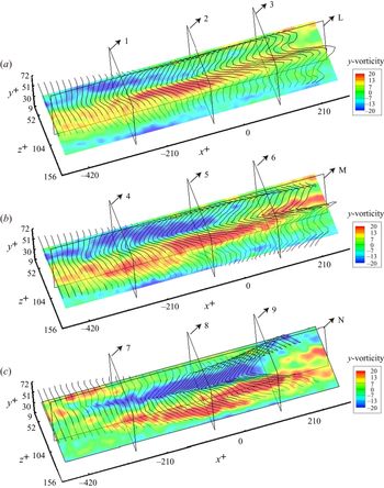
The vorticity distributions within the region of LSS-II, corresponding to figure 6 (and also figures 11 and 12) are shown in figures 14 and 15, at  $t^+ = 131$, 151 and 170. The distributions of
 $\omega _y$ shown in figure 14 reveal the spanwise variation of
 $\omega _y$.
Evolution of wall-normal vorticity  $\omega _y$ in the region of LSS-II at
 $y^+=27$, shown superimposed with 3-D time-lines corresponding to figure 6: (a)
 $t^+=131$; (b)
 $t^+=151$; and (c)
 $t^+=170$. The planes numbered 1–9 are
 $y$–
 $z$ planes and the planes labelled L, M and N are
 $x$–
 $y$ planes, showing the location of the vorticity contours shown in figures 15 and 16.

Evolution of streamwise vorticity  $\omega _x$ on a series of
 $z$–
 $y$ planes. The slices labelled 1–9 and the superimposed time-lines are the same as those shown in figure 14. (a) Colour contours of
 $\omega _x$ at
 $t^+=131$, as they appear respectively at
 $x^+ = -282$,
 $x^+ = -73$ and
 $x^+ = 105$. (b) Colour contours of
 $\omega _x$ at
 $t^+=151$, at the same respective locations as in (a). (c) Colour contours of
 $\omega _x$ at
 $t^+=170$, at the same respective locations as in (a).

The ‘peak–valley’ patterns of the superimposed 3-D time-lines initiated at  $y^+ = 27$ appear to coincide with concentrations of
 $\omega _y$, revealing two extended regions of positive and negative vorticity flanking LSS-II. As the two regions of opposing
 $\omega _y$ advect downstream, the accompanying time-lines become more warped and appear to display some streamwise rotation by
 $t^+ = 170$ (figure 14c).
The distributions of streamwise vorticity  $\omega _x$ in figure 15 show some concentrations of
 $\omega _x$ of opposing signs flanking the sides of the LSS. However, the regions of
 $\omega _x$ concentration do not show a strong coincidence with the time-lines. Figure 16 shows the distribution of spanwise vorticity
 $\omega _z$ at
 $z^+ = 89$, at the same time realizations as figures 14 and 15. While figures 14–16 show concentrations of vorticity adjacent to the streak, none of this concentration appears to take the form of rotational vortices. Analysis of the vorticity patterns for four other identified streaks shows essentially the same behaviour of vorticity distribution and type.
Evolution of spanwise vorticity  $\omega _z$ in the region of LSS-II at
 $z^+=89$, corresponding to the planes L, M and N in figure 14: (a)
 $t^+=131$; (b)
 $t^+=151$; and (c)
 $t^+=170$.

The distributions of wall-normal ( $y$) and streamwise (
 $x$) vorticity, as well as vortical behaviour detected using the median of the three eigenvalues of
 $\boldsymbol {\varOmega }^2+\boldsymbol{\mathsf{S}}^2$ (
 $\lambda _2$-criterion; Jeong & Hussain Reference Jeong and Hussain1995), are shown in figure 17 for LSS-II at
 $t^+ = 151$. Here
 $\lambda _2$ is the second eigenvalue of
 $\boldsymbol {\varOmega }^2+\boldsymbol{\mathsf{S}}^2$, where
 $\boldsymbol {\varOmega }=[\boldsymbol {\nabla }\boldsymbol {v}-(\boldsymbol {\nabla } \boldsymbol {v})^{\textrm {T}}]/2$ is the vorticity tensor and
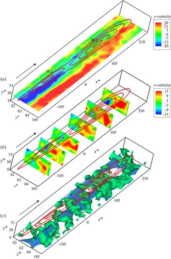
 $\boldsymbol{\mathsf{S}}=[\boldsymbol {\nabla } \boldsymbol {v}+(\boldsymbol {\nabla } \boldsymbol {v})^{\textrm {T}}]/2$ is the rate-of-strain tensor. The vorticity distributions of figure 17(a) and (b) are shown as colour contours, superimposed on red line contours representing the deformed material surface of LSS-II shown in figure 13(d). Figure 17(a) reflects opposing-sign wall-normal vorticity extending in the
 $x$-direction, and flanking the streak region. The opposing-sign vorticity flanking the trailing wave, W2, is more balanced than that adjacent to the leading wave, W1. Figure 17(b) indicates that streamwise vorticity,
 $\omega _x$, is concentrated to the sides of the streak, with the positive vorticity (right side) much stronger than the negative vorticity (left side), as indicated by the larger red area on the right. The regions of negative streamwise vorticity (left side) also do not appear to be contiguously connected.
Vorticity and vortices in the region of LSS II. (a) Colour contours of wall-normal vorticity  $\omega _y$ on an
 $x$–
 $z$ plane at
 $y^+ = 27$, shown juxtaposed with contour lines of the deformed material plane shown in figure 13(d). (b) Colour contours of streamwise vorticity
 $\omega _x$ on a series of
 $z$–
 $y$ planes, again shown with the deformed material surface contour lines. Symbols A, B, C, D, E and F denote a
 $z$–
 $y$ plane at
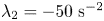
 $x^+ = -125, -73, -23$, 42, 105 and 165, respectively. (c) Vortices (green) are visualized for an isosurface of
 $\lambda _2 = -50\ \textrm {s}^{-2}$. The blue surface indicates a streamwise velocity of
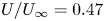 $U/U_\infty =0.47$.

Figure 17(c) shows the region identified as vortices (green) using the  $\lambda _2$-criterion with
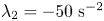 $\lambda _2=-50\ \textrm {s}^{-2}$. In figure 17(c), the blue surface reflects the LSS visualized by an isosurface of
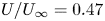 $U/U_\infty = 0.47$. From this figure, there appear to be vortical arch structures straddling the streak, although there is not much evidence of streamwise trailing legs for these arch structures/vortices. Additionally, the arch structures do not appear to develop into contiguous hairpin-type vortices, and the
 $\lambda _2$-identified structures appear to be distributed erratically.
It is difficult to directly determine the cause and effect between LSSs and vortices. This is because there is no general definition of vortices, which means that it is hard to distinguish whether the vorticity concentration is caused by a high-shear layer or vortices. Recently, an  $\varOmega$-criterion was proposed to deal with this issue (Liu et al. Reference Liu, Wang, Yang and Duan2016; Tian et al. Reference Tian, Gao, Dong and Liu2018), wherein
 $\varOmega$ is defined as a ratio of the vortical vorticity over the total vorticity:
 $\varOmega \approx b/(a+b+\epsilon )$, with
 $a=\textrm {trace}(\boldsymbol{\mathsf{A}}^{\textrm {T}}\boldsymbol{\mathsf{A}})$,
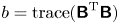 $b = \textrm {trace}(\boldsymbol{\mathsf{B}}^{\textrm {T}}\boldsymbol{\mathsf{B}})$ and
 $\epsilon$ is defined as a function of the maximum of the term
 $b-a$, proposed as
 $\epsilon = 0.001 (b-a)_{max}$. Note that
 $\boldsymbol{\mathsf{A}}$ and
 $\boldsymbol{\mathsf{B}}$ are the rate-of-strain tensor and the vorticity tensor, respectively, as mentioned above. When
 ${\varOmega } < 0.5$, only high-shear layers are indicated;
 $\varOmega = 0.52$ is generally adopted as approximately defining a vortex boundary. Figure 18 shows a snapshot of the distribution of
 ${\varOmega } >0.5$ (slices) and LSSs (grey isosurface). In figure 18, the black contour lines on the slices show vortex boundaries (
 $\varOmega = 0.52$), and the vortex cores are identified as the locations of
 $\varOmega$ maximum within the boundary. From figure 18, most of the
 $\varOmega$-identified structures, including strong vortices (where the maximum of
 $\varOmega$ is larger than 0.8), appear to be distributed erratically. This is similar to the distribution of streamwise vorticity shown in figure 15. However, the LSSs detected by the isosurface of
 $U/U_\infty =79\,\%$ seem much larger in size than the vortices, and there is little evidence that the lift-up of LSSs is the result of organized vortex interactions.
Snapshots of LSSs and vortex boundaries identified based on the  $\varOmega$-criterion (Liu et al. Reference Liu, Wang, Yang and Duan2016) at
 $t^+ = 152$. The grey surface shows the isosurface of
 $U/U_\infty =79\,\%$, with contour lines showing the wall-normal distance. Contours on the slices indicate the distribution of
 $\varOmega$ larger than 0.5, with black contour lines showing the boundaries of vortices (
 $\varOmega =0.52$).

Figure 19 shows the distribution of  $\varOmega$-based vortices near the LSSs. Figure 19(a) shows the statistical distribution of vortices relative to their spanwise distance from the centre of the nearest LSS in the same
 $y$–
 $z$ plane. The position of the vortex was identified according to the maximum of
 $\varOmega$ within the boundary of
 ${\varOmega } = 0.52$, and the centre of the LSS was identified as the highest region of the isosurface of U/
 $U_\infty =79\,\%$. Figure 19(a) indicates that most of the vortices flank the sides (indicated by P1 and P2 in the distribution) of LSSs in closer proximity to the centre of the LSS. Almost 90 % of the vortices are within a distance of
 $|{\rm \Delta} z^+|<50$, which is not surprising, considering that the spanwise spacing of two neighbouring LSSs in most of cases is
 $\textrm {d} z^+ \approx 100$.
(a) Histogram showing the distribution of vortices ( $n$) according to their distance from the centre of the nearest LSS (
 $\textrm {d} z^+$). (b) Scatter plot of the strength of vortices (
 $\varOmega _{max}$) and their distance to the centre of the nearest LSS (
 $\textrm {d} z^+$);
 $\varOmega _{max}$ is the maximum of
 $\varOmega$ at the vortex core within the boundary of
 ${\varOmega } = 0.52$.

Figure 19(b) shows a scatter plot of the vortex strength ( $\varOmega _{max}$) relative to their distance from the centre of the nearest LSS (
 $\textrm {d} z^+$). The figure reveals no relationship between
 $\varOmega _{max}$ and
 $\textrm {d} z^+$ (correlation coefficient
 $r = -0.03$), which indicates that the lift-up of an LSS may not be due to the induction of organized vortices. If a vortex is identified as a strong vortex with
 ${\varOmega }_{max}>80$, then figure 19(b) shows that 80 % of the identified vortices are not strong vortices (green filled markers in figure 19b). These vortices may be caused by the breakdown of a 3-D wave structure (LSS), or the result of streak instability (Jiménez & Moin Reference Jiménez and Moin1991). Note also that the vortices identified as strong (
 ${\varOmega }_{max}>$ 80, red filled markers) show no consistent or organized pattern that suggests that an LSS is the result of vortex interaction.
Based on our present results for an early turbulent boundary layer (the evolution of material surfaces/time-lines and vorticity distributions), it is reasonable to draw the conclusion that the formation and lift-up of an LSS are not the result of vortex interactions in the near-wall region. Because of the observed warping behaviour of the material surfaces shown in figures 10 and 12, we speculate that the initiation and development of LSSs is more likely the result of 3-D wave behaviour, the amplification and breakdown of which result in the initial streak bursting and generation of hairpin vortices. The vortex–streak interaction process is further examined in § 4.
4. Lagrangian vortices in proximity to LSSs
Most coherent structures in a turbulent boundary layer are vortices of one form or another, but there is no universal method for detecting these vortices. Some identification schemes are based on regions of high vorticity according to the instantaneous scalar field values (Hunt, Wray & Moin Reference Hunt, Wray and Moin1988; Chong, Perry & Cantwell Reference Chong, Perry and Cantwell1990; Jeong & Hussain Reference Jeong and Hussain1995; Chakraborty, Balachandar & Adrian Reference Chakraborty, Balachandar and Adrian2005), while others are based on a finite-time view considering a set of fluid trajectories (Haller Reference Haller2005; Shadden, Dabiri & Marsden Reference Shadden, Dabiri and Marsden2006; Green, Rowley & Haller Reference Green, Rowley and Haller2007; Haller et al. Reference Haller, Hadjighasem, Farazmand and Huhn2016). The latter approach defines a coherent vortex as a region with material invariance. In this paper, objective vortex determination is done using a criterion called Lagrangian-averaged vorticity deviation ( $LAVD$), based on the technique of Haller et al. (Reference Haller, Hadjighasem, Farazmand and Huhn2016). This technique is used in conjunction with the velocity field database to detect vortex boundaries and analyse the dynamics of the interaction between coherent vortices and LSSs.
The  $LAVD$ method was developed on the basis of dynamic polar decomposition (DPD; Haller Reference Haller2016), which separates the deformation gradient into two parts: the first representing the purely rotational part of the flow with zero rate of strain, and the second representing the purely strained part of the flow with zero vorticity. The
 $LAVD$ is defined by Haller et al. (Reference Haller, Hadjighasem, Farazmand and Huhn2016) as
 \begin{equation} LAVD^t_{t_0}(\boldsymbol{x}_0) := \int_{t_0}^{t} |\boldsymbol{\omega}(\boldsymbol{x}(s;\boldsymbol{x}_0),s) -\bar{\boldsymbol{\omega}}(s)| \,\textrm{d}s. \end{equation}
In (4.1),  ${\boldsymbol {x}}_0$ is the initial position of a specific fluid volume tracked from
 $t_0$ to
 $t$,
 $\boldsymbol {\omega }$ is the vorticity defined as
 $\boldsymbol {\nabla } \boldsymbol {\cdot } \boldsymbol {v}$, and
 $\bar {\boldsymbol {\omega }}$ is the instantaneous spatial mean vorticity over the material domain formed by a set of evolving trajectories, and is defined as
 \begin{equation} \bar{\boldsymbol{\omega}}(t) = \frac{\displaystyle\int_{M(t)}\boldsymbol{\omega}(\boldsymbol{x},t)\,\textrm{d}V}{\textrm{vol}({M(t)})}, \end{equation}
where  $M(t)$ is the material domain, and
 $\textrm {vol}$(
 $M(t)$) denotes the volume of the material domain for 3-D flows; if a 2-D flow is examined,
 $\textrm {vol}$(
 $M(t)$) would be the area of the material domain. The
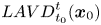 ${LAVD}^t_{t_0}(\boldsymbol {x}_0)$ field defined by (4.1) is a dynamically consistent and objective measure of bulk material rotation relative to the spatial mean rotation of the fluid volume
 $M(t)$. A rotationally coherent Lagrangian vortex is an evolving material domain
 ${M}(t)$, such that
 ${M}(t_0)$ is filled with a nested family of tubular level surfaces of
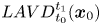 ${LAVD}^{t_1}_{t_0}(\boldsymbol {x}_0)$ with outward-decreasing
 $LAVD$ values. The
 $LAVD$-based vortex boundary,
 $\mathscr {B}(t)$, is defined as a tubular material surface that encloses a region of concentrated vorticity. This material surface is the outermost tubular level surface of
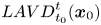 ${LAVD}^t_{t_0}(\boldsymbol {x}_0)$. Three conditions are required for a
 $\mathscr {B}(t)$: (1)
 $\mathscr {B}(t)$ encircles a vortex centre defined by the local maxima of
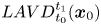 ${LAVD}^{t_1}_{t_0}(\boldsymbol {x}_0)$); (2)
 $\mathscr {B}(t)$ has an arclength exceeding a selected threshold; and (3)
 $\mathscr {B}(t)$ has a convexity deficiency less than a bounded value. Here, the convexity deficiency is defined as the ratio of the area between the boundary curve and its convex hull,
 ${A_b}$, to the area enclosed by the curve,
 ${A_i}$. For a more detailed description of the level-surface topology, we refer the reader to Haller et al. (Reference Haller, Hadjighasem, Farazmand and Huhn2016).
Figure 20(a) shows 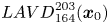 ${LAVD}^{203}_{164}(\boldsymbol {x}_0)$ contour lines, and the Lagrangian vortex boundaries detected in the
 $y$–
 $z$ plane, in the region adjacent to the location of LSS-I at
 $x^+ = -105$ and time
 $t^+=164$. Two apparent vortices are detected at
 $z^+\approx 19$ and
 $z^+\approx -50$, which are located to either side of LSS-I, originally shown in figure 5(a). The vortex core to the right (marked B in figure 20) has almost twice the
 $LAVD$ value as that of vortex core A. This means that the streamwise vorticity is more concentrated on the right side of the streak, within B. This is consistent with the asymmetric time-line patterns shown in figure 5(a–c). The red dashed lines shown on figure 20(a) and (b) are streamwise projections of the time-lines for LSS-I from figure 5(a) and (b). Since no strong roll-up of the time-lines was observed, the Lagrangian vortices shown in figure 20 are considered to be weak; this suggests that they represent the development of coherent structures at an early stage, which are not easy to detect from instantaneous time-line patterns. Figure 20(b) shows contour lines of
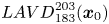 ${LAVD}^{203}_{183}(\boldsymbol {x}_0)$ at a farther downstream position of
 $x^+ = 0$ at time
 $t^+ = 183$. The time-lines at
 $t^+ = 183$ are also superimposed on figure 20(b). A comparison of figure 20(a) and (b) suggests that both the vortex A and vortex B grow from streamwise positions
 $x^+ = -105$ to
 $x^+ = 0$, and correspond to the more inflectional time-lines adjacent to the vortices. However, the persistence and dominance of the right vortex B results in a biasing of the time-lines to the right side of the streak.
End-view contours of  $LAVD$ and time-lines in the region adjacent to the location of LSS-I. (a)
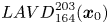 ${LAVD}^{203}_{164}(\boldsymbol {x}_0)$ at time
 $t^+=164$, location
 $x^+=-105$; red dashed lines are time-lines at
 $t^+=164$. (b)
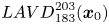 ${LAVD}^{203}_{183}(\boldsymbol {x}_0)$ at time
 $t^+=183$, location
 $x^+=0$; red dashed lines are time-lines at
 $t^+=183$. Flow direction is out of the plane of the paper.

The 2-D  $LAVD$ transverse contours of
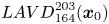 ${LAVD}^{203}_{164}(\boldsymbol {x}_0)$ and
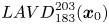 ${LAVD}^{203}_{183}(\boldsymbol {x}_0)$ in the
 $x$–
 $y$ plane at
 $z^+=-32$ are shown in figure 21(a) and (b). Superposed are the corresponding vertical time-line patterns (red dashed lines) as shown previously in figure 5(d–e). The
 $LAVD$-based vortex identified in yellow in the time realizations appears to deform and enlarge from time
 $t^+ = 164$ to 183. The locations of the vortex observed in figure 21(a) and (b) indicate that the vortex advects nearly parallel to the wall at the lower limit of the log-law region, rather than moving outwards away from the wall as is expected for hairpin vortices. As pointed out by Haidari & Smith (Reference Haidari and Smith1994), the hairpin vortex head is evidenced by the curvature of hydrogen bubble time-lines towards the middle of the vortex head. However, the Lagrangian vortices extracted here appear below the pronounced inflectional region, which appears in the time-line pattern of figure 21 at approximately
 $y^+ \approx 40\text {--}50$. The advection speed of the vortex is approximated from the relative positions of the vortex core in figure 21(a) and (b), as 59 % of
 $U_\infty$, which is similar to the streamwise velocity of the wave structure calculated from the material surface translation of figure 13, i.e. 65 % of
 $U_\infty$. This suggests that the vortex shown in figure 21 may be an initial vortex developing at the interface between the lifted-up wave structure (LSS) and the wall-ward high-speed flows.
Side-view contour of  $LAVD$ and time-lines in the region adjacent to the location of LSS-I. (a)
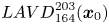 ${LAVD}^{203}_{164}(\boldsymbol {x}_0)$ at time
 $t^+=164$ and
 $z^+=-32$ (LSS-I). The superimposed red dashed lines are vertical time-lines at
 $t^+=164$, corresponding to figure 5(d). (b)
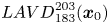 ${LAVD}^{203}_{183}(\boldsymbol {x}_0)$ at time
 $t^+=183$ and
 $z^+=-32$. The superimposed red dashed lines are vertical time-lines at
 $t^+=183$, corresponding to figure 5(e).

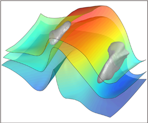
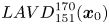
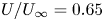
Figure 22(a) shows, for LSS-II, the 3-D Lagrangian coherent vortices (LCVs) extracted using 3-D  $LAVD$ contours, which are superimposed with the streamwise iso-velocity contour surface, and figure 22(b) shows the deformed material surface determined previously in figure 13(d). In figure 22(a), an isosurface of
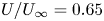 $U/U_\infty = 0.65$ at
 $t^+ = 151$ (coloured blue) is a conventional Eulerian representation of an LSS, similar to techniques employed in several previous investigations (Elsinga et al. Reference Elsinga, Kuik, van Oudheusden and Scarano2007; Gao et al. Reference Gao, Ortiz-Dueñas and Longmire2013). This isosurface takes on a hump-shaped appearance. Two quasi-streamwise vortices extracted from
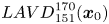 ${LAVD}^{170}_{151}(\boldsymbol {x}_0)$ (the initial domain
 $\boldsymbol {x}_0$ spans from
 $x^+ = -105$ to
 $210$) flank the sides of the apparent LSS, but vary in wall-normal and streamwise positions. The head of vortex A is slightly inclined, which is similar to the bull's horn-like vortex tube observed for a transitional boundary layer by Wortmann (Reference Wortmann1981). The wall-normal
 $y^+$ range for vortex A is
 $45\text {--}56$, and it is
 $23\text {--}47$ for vortex B. Vortex B is noticeably larger and stronger than vortex A, with its tail located at almost the same streamwise position as the head of vortex A, as shown in figure 22(b). A comparison with the streamwise vorticity distribution shown in figure 15 suggests that these two vortices are possibly two individual quasi-streamwise cane-shaped vortices that arise from the LSS. Similar, but more complicated, cane vortices were also observed in the tomo-PIV results of Elsinga et al. (Reference Elsinga, Kuik, van Oudheusden and Scarano2007), based on a
 $Q$-criterion analysis. These cane-shaped vortices are most often observed above the buffer layer, and are considered to originate from a sinuous instability of LSSs (Schoppa & Hussain Reference Schoppa and Hussain2002; Stanislas Reference Stanislas2017).
(a) The 3-D LCVs (green) extracted using 3-D  $LAVD$ contours of
 ${LAVD}^{170}_{151}(\boldsymbol {x}_0)$ in the region of LSS II at
 $t^+=151$, superimposed with the streamwise iso-velocity contour surface of
 $U/U_\infty =0.65$ (blue). (b) The material surface of figure 13(d).

In figure 22(b), the two Lagrangian vortices are remarkably coincident with the two humps of the material surface previously determined in figure 13(d). This appears to support the conjecture that cane vortices are generated in proximity to an LSS, or more precisely on the flanks of 3-D waves. It may be argued that the two humps in the LSS (apparent wave structures) are induced by the vortices. However, the evolution of the material surface shown in figures 12 and 13 clearly displays that the 3-D wave structures are much larger than the cane vortices, and further examination of material surface development initiating farther from the wall shows that the 3-D wave behaviour extends from the very near-wall region to  $y^+\approx 80$. In addition, the highest vertical velocity of the wave structures occurs in the near-wall region (
 $y^+<20$) rather than adjacent to the streamwise vortices. The instantaneous vorticity field results of figures 14–17, as well as the results from the 2-D
 $LAVD$, all support the conclusion that 3-D wave structures associated with LSSs are what give rise to the streamwise vortices, and not vice versa.
Figure 23 shows three temporal realizations of material surfaces and their associated LCVs for LSS-II, in both oblique views (top row) and end views (lower row). These realizations show the evolution and interaction of the material surfaces and the detected vortices over a time span  $t^+ = 151\text {--}170$. As time evolves, vortex A rotates anticlockwise and moves upwards as it advects downstream, apparently retaining its horn-like shape. Vortex B rotates clockwise, and undergoes what appears to be significant stretching, which intensifies the vortex and reduces the apparent vortex core (see figure 23d–f). During the advection of vortex B, it shrinks in size, which results in the initial multiple lobes (figure 23a) on the vortex boundary evolving into one distinct filament that strongly entrains the material surface (figure 23c,f). The material surfaces at
 $t^+=151$ (figure 23a) were initiated at
 $t^+ = 131$, and are reflective of a wave-like behaviour in the region adjacent to the location of LSS-II. The peak (labelled P in figure 23) of the material surfaces moves upwards as time evolves, with the flanks of the material surfaces becoming more distorted during the lift-up process, which indicates that an interaction occurs between the LCVs and the wave-like structure.
Spatio-temporal evolution of LCVs, initially extracted from 3-D 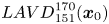 ${LAVD}^{170}_{151}(\boldsymbol {x}_0)$ field (grey), in comparison with the evolution of three material surfaces (labelled 1, 2 and 3), initiated at
 $t^+=131$ and
 $y^+=27$, 39 and 49 in the region adjacent to the location of LSS-II. (a–c) Oblique views of LCVs and material surfaces as they appear respectively at (a)
 $t^+=151$, (b)
 $t^+=161$ and (c)
 $t^+=170$. (d–f) End views (looking upstream) of LCVs and material surfaces as they appear respectively again at (d)
 $t^+=151$, (e)
 $t^+=161$ and (f)
 $t^+=170$.

5. Discussion
The results of the present study suggest that LSSs may be characterized as propagating 3-D wave motions accompanied by ejection and sweep behaviour. The ‘tomographic visualization’ results appear to be in accord with hydrogen bubble line visualizations, which suggests that the kink structure in vertical time-line patterns is consistent with the development of an incipient 3-D wave, which evolves into an amplified wave structure as it advects downstream. A hypothesized model of the bursting process, juxtaposed on an experimental image of LSSs, is shown in figure 24. The LSSs shown in figure 24(a) are reconstructed from tomo-PIV datasets at  $y^+ = 30$, and the hypothesized bursting process is characterized as a combined process of LSS ‘ejection’ and HSS ‘sweep’, as shown in figure 24(b).
Turbulent bursts at LSS: (a) ‘tomographic visualization’ of LSSs and high-speed region; (b) schematic view of physical behaviour of burst in low-speed region (adapted from Smith Reference Smith1998).

Smith (Reference Smith1984) proposed that the bursting process of an LSS involves vortex roll-up of the unstable shear layer formed on the top and sides of an LSS. The process consists of four stages: (1) lift-up and oscillation of an LSS; (2) initiation of vortex roll-up; (3) vortex development/amplification and concentration; and (4) vortex ejection, stretching and interaction. The first stage was explained by the growth of the LSS in the presence of an impressed local adverse pressure gradient, which leads to local fluid deceleration and development of a 3-D inflectional profile. Once an inflection develops, the streak will become locally unstable, precipitating a breakdown, conceptualized as a burst. However, the origin of the LSS and the origin of the local adverse pressure gradient were not identified. It was hypothesized by Smith (Reference Smith1984) that the passage of a vorticity concentration created upstream can create a transient, spatially varying pressure gradient, which could precipitate the local deceleration. That is supported by the classical kernel studies of isolated vortices, such as the hairpin vortex shedding from a hemisphere protuberance being shown to precipitate downstream fluid ejections from near the bounding wall (Acarlar & Smith Reference Acarlar and Smith1987a,Reference Acarlar and Smithb).
However, for a boundary layer on a smooth flat plate without impressed disturbances, the natural process that causes the development and breakdown of LSSs is not readily apparent. In order to address that question, we will consider the process of transition in an initially laminar boundary layer (e.g. Hama & Nutant Reference Hama and Nutant1963; Jiang et al. Reference Jiang, Lee, Chen, Smith and Linden2020); see also appendix B.1 and B.3. A comparison of the time-line patterns for a controlled transitional boundary layer reveals markedly similar patterns to those for LSSs in a turbulent boundary layer (figures 4 to 6). This suggests that the process and the structures developing in the transitional boundary layer may reflect a similar process and structure in the near-wall turbulent boundary layer. In previous studies, spikes were found in the late-stage transition, and they were found to originate from the high-frequency secondary instability (Nishioka et al. Reference Nishioka, Asai and Iida1981; Nishioka & Asai Reference Nishioka and Asai1984). A chain of ring-like vortices (termed CS-soliton) was also suggested to explain the spikes in the outer part of the boundary layer (Kachanov Reference Kachanov1994; Borodulin et al. Reference Borodulin, Gaponenko, Kachanov, Meyer, Rist, Lian and Lee2002).
The model of Smith (Reference Smith1984) is similar to the concept of an instability-induced hairpin scenario of Nishioka et al. (Reference Nishioka, Asai and Iida1981) and Hack & Moin (Reference Hack and Moin2018), which attributed the origin of hairpin vortices to the instability of LSSs. The studies of streak instability have shown that a varicose instability of an LSS is able to create arch vortices, and the sinuous instability of an LSS produces quasi-streamwise vortices on the sides of the LSS. The wave structure within the LSS observed in the present study may be a manifestation of a varicose instability of an LSS. The wave-like undulation of an LSS (varicose instability) in turbulent boundary layers leads to a wave-like vorticity concentration and a local 3-D high-shear layer, which are considered as the necessary conditions for the development of a hairpin vortex (or arch vortex). As noted in Schoppa & Hussain (Reference Schoppa and Hussain2002), the transient growth of streaks can generate the well-documented structures near the wall from an initially quiescent streak region containing no initial vortices. The growth of a wave-like LSS as suggested by this study may reflect a transient growth process because the proper streamwise wavelength of the streak ( $l^+$) is close to the most amplified disturbance calculated from the liner stability by Schoppa & Hussain (Reference Schoppa and Hussain2002). But this, of course, needs further investigation.
There is another perspective of LSS behaviour, which considers an LSS as a combined structure of several wave structures (termed soliton-like coherent structure; SCS), where these wave structures are proposed to be the initiators of hairpin vortices in transitional boundary layers, as well as turbulent boundary layers (Lee Reference Lee1998; Lee & Wu Reference Lee and Wu2008; Chen Reference Chen2013; Jiang et al. Reference Jiang, Lee, Chen, Smith and Linden2020). In addition, the results of a DNS study of the transition of channel flow by Zhao et al. (Reference Zhao, Yang and Chen2016) observed that, prior to the appearance of a signature hairpin-like structure, a triangular bulge similar to an SCS forms, followed by vorticity intensification and roll-up of a vortex sheet near the bulge ridges. Such a triangular bulge was also observed before the inception of turbulent spots by Zhao et al. (Reference Zhao, Xiong, Yang and Chen2018). The material surfaces and time-line patterns obtained in the vicinity of LSSs for the present study also manifest as a bulge, the ridges of which begin to roll up as time evolves. The vorticity distributions shown in figures 14 and 15 confirm vorticity intensification in the region of the triangular ridges. Thus, we propose a wave-induced scenario for the generation of LSSs and hairpin vortices in a turbulent boundary layer. The details of this wave-induced process are modelled in figure 25.
A sequenced model of the hypothesized temporal development of a 3-D wave structure, leading to subsequent vortex generation.

It is hypothesized that a 3-D wave, appearing as a warped wave front (Jiang et al. Reference Jiang, Lee, Chen, Smith and Linden2020), develops as a nonlinear interaction of a pair of opposing-angle oblique waves as are observed in boundary layer transition (see figure 30). As the generated 3-D wave travels downstream at a speed of approximately 65 %  $U_\infty$, it moves upwards to retard the outer fluid, similar to the action of a pulsed wall jet. This deflection of the outer fluid results in a local change in the pressure gradient, as well as creating inflections in the streamwise and transverse velocities. The result is the development of a 3-D inflectional profile, as depicted in Smith (Reference Smith1984). As the fluid encompassed by the 3-D wave moves upwards, the surrounding flow is displaced downwards due to mass conservation. During this process, the differential in flow velocities between the wave and the downward-moving fluid will create a high-shear interface at the 3-D wave boundaries, shown as stage A in figure 25. The lift-up speed for the 3-D wave is maximum in the near-wall region, and, as the wave moves upwards within the boundary layer, it will deform into an inclined 3-D wave as it encounters higher-velocity fluid at its crest, shown as stage B in figure 25. The ejections and sweeps that are stimulated by the 3-D wave lift-up create a high-vorticity, 3-D shear layer encompassing the wave, which subsequently breaks down, rolling up into hairpin or other vortices. This process is similar to the advected instability caused by the 3-D separation from a hemisphere or a transverse fluid injection from the wall (Acarlar & Smith Reference Acarlar and Smith1987a,Reference Acarlar and Smithb; Sabatino & Rossmann Reference Sabatino and Rossmann2016).
The so-called ‘vorticity concentrations’ in the low-momentum streak region (Smith Reference Smith1984) or the ‘vorticity intensification’ near the bulge ridge (Zhao et al. Reference Zhao, Yang and Chen2016) may be caused by the ejection of the 3-D wave structure according to vorticity transfer theory (Wu, Ma & Zhou Reference Wu, Ma and Zhou2015). The initial vortex roll-up caused by the lift-up and the resultant wall-ward sweep motions are presumed to be inclined at an angle to the wall, as modelled by the ‘initial roll-up’ shown in stage B of figure 25. It is also presumed that the inrush-induced shear layer near the lower trailing portion of the wave will be weak due to the background shear, and thus the initial vortex roll-up will appear as a  $\Lambda$-shaped vortex. Once the vortex roll-up develops along the high-shear boundaries of the 3-D wave, the vortex will then shed and be stretched into a hairpin vortex, as shown in stage C of figure 25. This shedding and stretching process is dominated by self-induced motions and viscous–inviscid mechanisms, resulting in subsequent vortex ejection, stretching and interaction. Note that the model shown in figure 25 is an idealized process, for which the vortices develop symmetrically without consideration of other events occurring in proximity to the wave, which will, of course, have a secondary influence on their behaviour.
It is known that most vortices detected in turbulent boundary layers are asymmetric, and appear predominantly as distorted one-legged hairpins or cane-like structures (Robinson Reference Robinson1991; Smith et al. Reference Smith, Walker, Haidari and Sobrun1991; Adrian Reference Adrian2007; Dennis & Nickels Reference Dennis and Nickels2011; Stanislas Reference Stanislas2017). These vortex characteristics are also supported by the results of the present study. However, the Eulerian assessment using time-line and vorticity distributions shown in figures 14–19 reveal no apparent large-scale vortices associated with the LSSs. However, using a Lagrangian assessment via  $LAVD$ processing, quasi-streamwise vortices adjacent to the 3-D waves were detected, which are speculated to arise from initial vortex roll-ups evolving from the high-shear layer interface of the 3-D wave. The reason the
 $LAVD$ method can detect these vortices is that Lagrangian methods inspect and trace a domain of fluid for a finite time, from which it is easier to extract the dominant flow structures, and with less effect of extraneous noise.
LSSs are abundant in bypass transition, and are similar to the flow topology of LSSs in turbulent boundary layers. Streak breakdown in bypass transition has been studied experimentally (Matsubara & Alfredsson Reference Matsubara and Alfredsson2001; Asai et al. Reference Asai, Konishi, Oizumi and Nishioka2007; Mans, de Lange & van Steenhoven Reference Mans, de Lange and van Steenhoven2007) and using simulations (Brandt & Henningson Reference Brandt and Henningson2002; Wu & Moin Reference Wu and Moin2010). A sinuous streak instability mode developing into a train of streamwise vortices is commonly observed. From an instability viewpoint, the streak breakdown into hairpin vortices in the present study seems to be due to the varicose instability of the 3-D high-shear layer lifted away from the wall. This process is manifested as the lift-up and amplification of a 3-D wave-like structure in a Lagrangian perspective. This observation is different from the ubiquitous sinuous instability of LSSs in bypass transition.
Recently, Wu et al. (Reference Wu, Moin, Wallace, Skarda, Lozano-Durán and Hickey2017) proposed the presence of transitional–turbulent spots (TRTSs) and turbulent–turbulent spots (TUTSs) in boundary layers. The inception mechanism of TRTSs in bypass transition is analogous to the secondary instability of natural boundary layer transition (Nishioka et al. Reference Nishioka, Asai and Iida1981). However, Wu et al. (Reference Wu, Moin, Wallace, Skarda, Lozano-Durán and Hickey2017) determined that the existing TRTSs will influence the meandering, waviness and breakdown of long streaks, although the streaks are not the mechanisms for the inception of TRTSs. Zhao et al. (Reference Zhao, Xiong, Yang and Chen2018) used a Lagrangian-based structure-identification method to study the inception of turbulent spots and their lateral growth. They observed that the vortex surface, in the inception of TUTSs, first forms a triangular bulge and then evolves into the primary hairpin-like structure by a rolling up of the lateral edges of the bulge. The roll-up of the hairpin-like bulges further induces sinuous spanwise perturbations and triggers a Kelvin–Helmholtz instability in the spanwise direction. The vortex surface deformation is similar to the initial deformation of temperature isosurfaces during the initial formation of TUTSs (Wu et al. Reference Wu, Moin, Wallace, Skarda, Lozano-Durán and Hickey2017). The triangular bulge observed in bypass transition (Wu et al. Reference Wu, Moin, Wallace, Skarda, Lozano-Durán and Hickey2017; Zhao et al. Reference Zhao, Xiong, Yang and Chen2018) and also K-regime transition (Zhao et al. Reference Zhao, Yang and Chen2016) appears similar to the wave-like structures of the streaks observed in the present study (e.g. figure 11). This suggests that a similar 3-D wave amplification behaviour of the LSSs is responsible for the generation of wall-region hairpin and other types of vortices in turbulent boundary layers. The spanwise meandering of the LSSs (figure 8b), which can be as much as 50 wall units, documented and discussed in § 4 and also by Zhao et al. (Reference Zhao, Xiong, Yang and Chen2018), is speculated to be the result of subsequent streak–vortex interactions.
Once a hairpin vortex develops (including its asymmetric types), it will induce fluid near the bounding surface to lift up and promote the ejection of the 3-D wave, which may be construed as the bursting process in a developed turbulent boundary layer. This may unify the two general concepts applied to the term ‘bursting’ (Robinson Reference Robinson1991), in that this model suggests that the development of both local instabilities and quasi-streamwise vortices are associated with 3-D waves. It is hypothesized that low-momentum fluid developing between the legs of hairpin vortices (or adjacent to quasi-streamwise vortices) combine with fluid ejected by the breakdown of the 3-D wave to form further low-speed regions (Adrian Reference Adrian2007; Hack & Moin Reference Hack and Moin2018). The continued quasi-periodic generation of hairpin vortices by this breakdown of 3-D waves will result in the development of hairpin packets by a complicated process of self-induction and vortex interactions, which will subsequently result in the generation of larger uniform-momentum zones. Additionally, the interaction of the initially generated vortices with subsequent 3-D waves can act as a perturbation to cause continued wave breakdown, resulting in continued regeneration of hairpin-like vortices, and providing the mechanism for sustaining wall-bounded turbulence.
6. Conclusion
In the present paper, the near-wall structures of an early turbulent boundary layer have been investigated using time-line and material surface visualization synthesized from a POD-filtered tomo-PIV, as well as identification of Lagrangian coherent vortices (LCVs) using Lagrangian-averaged vorticity deviation ( $LAVD$). The time-line visualizations confirm that LSSs are spaced with
 ${\rm \Delta} z^+ \approx 100$ and the bursting process is observed to comprise ejection–sweep events.
The 3-D evaluation of the tomographic time-lines demonstrates that the so-called bursting process is closely associated with 3-D wave behaviour of LSSs. A wave-induced burst is observed to consist of a slow lift-up of near-wall fluid, followed by an amplification and breakdown. The spatio-temporal deformation of advected material surfaces (figures 10, 12 and 13) reveals a 3-D wave behaviour of the LSS, with the subsequent breakdown resulting in ejections and sweeps associated with the bursting process. As shown by the evolution of material surfaces at varying distances from the wall, the 3-D wave structure propagates downstream at a speed of nearly 65 % of the free-stream velocity, determined by the wave crest movement, which is essentially the same speed as that determined by tracking the kinked band visualizing a streak within the time-line patterns. The maximum upward velocity of a 3-D wave, as determined by the translation of wave crests, is nearly  $6\,\%$ of the free-stream velocity at
 $y^+ < 49$, decreasing as the wave moves away from the wall. The vorticity distribution results appear to support the hypothesis that 3-D wave amplification is the active process that leads to the development of LSSs, and not the result of vortex interactions.
To further investigate the relationship between LSSs and vortices, both 2-D and 3-D  $LAVD$ (Haller et al. Reference Haller, Hadjighasem, Farazmand and Huhn2016) were applied to near-wall regions where LSSs were present. These vortices are identified as roll-ups occurring adjacent to the high-shear interface of 3-D waves on a streak, but which are not mature enough to evolve into a hairpin vortex. These detected
 $LAVD$ vortices also support the hypothesis that hairpin vortices originate from the unstable high-shear layer generated at the interface between lifted-up low-speed, near-wall fluid and downward sweeps of high-speed log-region fluid (Haidari & Smith Reference Haidari and Smith1994), and are not the cause of such lift-ups.
Large-scale quasi-streamwise vortices detected using the 3-D  $LAVD$ criterion show that such vortices develop adjacent to the lateral sides of an LSS. These cane-like streamwise vortices are hypothesized to be generated by the amplification and breakdown of the 3-D wave behaviour of the LSS.
The present study suggests that LSSs appear to evolve as 3-D waves. These 3-D waves, with low advection speed (60–80 % of  $U_\infty$), are hypothesized to have their origin in the near-wall fluid, creating an interfacial shear layer with higher-speed outer fluid, similar to soliton-like coherent structures (Lee Reference Lee1998; Lee & Wu Reference Lee and Wu2008). The process results in the generation of local 3-D pressure gradients, and the subsequent wave-like amplification of the shear layer.
The burst sequence model observed by the present study is similar to that hypothesized by Smith (Reference Smith1984). However, we suggest that the oscillation and undulations of an LSS, as well as the initial breakdown and roll-up to form vortices, are products of the streak behaving as a 3-D wave, within the near-wall fluid. The initial breakdown and roll-up of an LSS will develop along the bounding high-shear layer of the 3-D waves. These shear layers will subsequently evolve into several inclined vortices adjacent to the waves, which will further develop into hairpin-like or other vortices. The vortices observed in the viscous wall region usually manifest themselves as quasi-streamwise vortices. Thus, the two general concepts of the term ‘bursting’ by Robinson (Reference Robinson1991) may be unified, in that the development of streak instability and the generation of quasi-streamwise vortices may both be associated with 3-D waves.
It must be admitted that establishing the framework of coherent structures and extracting their cause and effect within a turbulent boundary layer is a formidable challenge. The joint theoretical and experimental efforts of investigators have resulted in many classical models, although some of them display many discrepancies. The present study has attempted to understand the process of development and breakdown of LSSs, and the associated bursting behaviour within the near-wall region at low Reynolds number ( $y^+ < 100$). The models proposed in this paper are not free from bias, but the ideas are initiated and motivated by the work of many respective researchers. In developing our present model of near-wall turbulent behaviour, we have tried to rectify the results of previous studies with the results and observations of the present study. We hope that our results and perceived model of near-wall turbulence will facilitate a better understanding of turbulent boundary layer behaviour.
Acknowledgements
The authors would like to express great appreciation to Professor J. Z. Wu, Professor Y. Yang and Professor S. I. Chernyshenko for their valuable and constructive advice. The authors gratefully acknowledge Professor K. Matsuura for providing a DNS database. The authors are also grateful to Dr Y. Zhu, Dr X. Chen, Dr A. Gao and Dr C. Xiong for valuable discussions on this research work. This work was supported by the National Natural Science Foundation of China (10921202, 11221061, 11632002, 11521091 and 11602005) and National Key Project GJXM92579.
Declaration of interests
The authors report no conflict of interest.
Appendix A. POD analysis and the low-order representation
Pre-processing of the experimental data is necessary due to the experimental noise within the velocity field. For a turbulent boundary layer, Wu (Reference Wu2014) pointed out that instantaneous large-scale turbulence structures are the main contributors to the first two POD modes based on analysis of a 2-D PIV dataset. Deng et al. (Reference Deng, Pan, Wang and He2018) also determined that the first four leading-order POD modes jointly depict the downstream convection of the large-scale ejection/sweep events, which were regarded as the low-order imprints of the hairpin packets. The decomposition can be written as
 \begin{equation} \boldsymbol{V}(\boldsymbol{X},t) = \sum_{i=1}^{N_t}{a_i(t)\varPhi_i(\boldsymbol{X})}, \end{equation}
in which  $\boldsymbol {V}(\boldsymbol {X},t)$ is the vector field with its temporal mean subtracted,
 $\varPhi _i(\boldsymbol {X})$ is the eigenmode of the ith mode,
 $a_i$ is the mode's time coefficient, and
 $N_t$ is the snapshot number selected in the set.
For a turbulent boundary layer, the mean flow contains the most of energy (nearly 95 % of the total energy in the present study). The energy distribution for the  $N_t$ POD modes for instantaneous velocity fluctuation is shown in figure 26 for selected
 $N_t$. Here, the energy
 $E_n$ is represented by
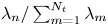 $\lambda _n/\sum _{m=1}^{N_t}\lambda _m$, with
 $\lambda _n$ being the corresponding eigenvalue. The notation
 $[{a\kern0.5pt{:}\kern0.5pt\textrm {d} t\kern0.5pt{:}\kern0.5pt b}]$ in the legend indicates the subset
 $[a,b]$ with a spacing
 $\textrm {d} t$ selected for POD analysis. Figure 26 shows that the energy rapidly decays with increasing mode number. The sum of the energy for the first four modes for case
 $[1\kern0.5pt {:} \kern0.5pt1\kern0.5pt {:} \kern0.5pt 999]$ is approximately 11 % of the total energy. However, this value increases to 23 % for the case
 $[1\kern0.5pt {:} \kern0.5pt 1\kern0.5pt {:} \kern0.5pt 250]$. This change may be the result of different inherent flow structures being present within the selected range of the dataset. It is known that wall-bounded turbulence is characterized by intermittency and a bursting process. If a dataset is selected for a period of the breakdown of flow structures, there will be no apparent large flow structures within the field, leading to a relatively low energy at low-order POD modes. The energy of low-order modes also changes when different subsets of the flow are selected even for nearly the same snapshot number, as shown by the lines with triangular markers in figure 26. But the sum energy of the first four modes for these cases (
 $[1\kern0.5pt {:} \kern0.5pt 1\kern0.5pt {:} \kern0.5pt 250]$ and
 $[751\kern0.5pt {:} \kern0.5pt 1\kern0.5pt {:} \kern0.5pt 999]$) are very close to each other, nearly 25 % of total energy. However, the flow field approximated from the first four POD modes based on the dataset of
 $[1\kern0.5pt {:} \kern0.5pt 1\kern0.5pt {:} \kern0.5pt 999]$ and the subset of
 $[751\kern0.5pt {:} \kern0.5pt 1\kern0.5pt {:} \kern0.5pt 999]$ are markedly similar. This indicates that the energy distribution of POD modes relies mainly on the selected dataset, and it has little effect on the extraction of large-scale structures of the flow field.
Energy distribution of the POD modes for different selected sizes of the POD sample ( $N_t$).

The flow field can be represented in terms of the finite or truncated series only within the first  $r$ modes (Taira et al. Reference Taira, Brunton, Dawson, Rowley, Colonius, McKeon, Schmidt, Gordeyev, Theofilis and Ukeiley2017). Lower-rank approximations of the velocity field at
 $y^+=30$ and
 $t^+=164$ are shown in figure 27(a–c), with
 $r$ being selected as 80, 22 and 4, respectively. A comparison of panels (a–c) in figure 27 shows that the velocity field based on POD approximation from the first four leading-order POD modes contains less small structures, while retaining the large-scale structures. Low-speed streaks represented by an isosurface of
 $u/U_\infty = 73.5\,\%$ (blue regions) are shown in figure 27(d) and (e), for both the original velocity field after a Gaussian smoothing with
 $5\times 5\times 5$ vectors and for a POD-approximated field with
 $r=4$, respectively. A comparison of figure 27(d) with figure 27(e) shows that POD is effective for retaining the larger-scale LSSs. Figure 2(b) shows the effect of the POD filtering of PIV on fluctuating velocity profiles. The underestimation of streamwise velocity fluctuation
 $u^{\prime}$ is 40 % in the vicinity of the wall, while the underestimation of
 $v^{\prime}$ can be as high as 80 %. This indicates that the method of low-order approximation based on the first four POD modes is similar to an appropriate filtering with a large box filter as is commonly used for turbulent shear flows (Atkinson et al. Reference Atkinson, Buchmann, Amili and Soria2014).
Streamwise velocity contours at  $y^+=30$ and
 $t^+=164$, based on different POD approximations: (a) POD approximation based on the first 80 leading-order POD modes; (b) POD approximation based on the first 22 leading-order POD modes; (c) POD approximation based on the first four leading order POD modes; (d) original flows field after a Gaussian smoothing filter with
 $5\times 5\times 5$ vectors, superimposed with an isosurface of
 $u/U_\infty = 73.5\,\%$; (e) POD approximation based on the first four leading-order POD modes, superimposed with an isosurface of
 $u/U_\infty = 73.5\,\%$ (blue region).

Appendix B. Lagrangian tracking based on marked particles
It is almost impossible for traditional hydrogen bubble time-line visualization to directly reveal 3-D flow behaviour from different simultaneous viewing angles. It is also difficult to differentiate between a wave structure and a complex vortical flow. Reconstruction of time-line patterns has proven effective and useful for assessing the spatio-temporal characteristics of boundary layers, and the detection of coherent flow structure (Laurien & Kleiser Reference Laurien and Kleiser1989; Bernard Reference Bernard2013; Jiang et al. Reference Jiang, Lee, Chen, Smith and Linden2020). For 3-D velocity datasets, the position of each particle at different time steps can be determined by integrating an ordinary differential equation (ODE) over real time:
 \begin{equation} \boldsymbol{V}(\boldsymbol{X}(t),t) = \textrm{d}\boldsymbol{X}(t)/\textrm{d} t. \end{equation}
In the present study, a MATLAB algorithm that employs an ODE solver and interpolation scheme was used to generate patterns based on the movement of marked particles in a 3-D velocity dataset. In order to generate time-lines similar to hydrogen bubble time-lines, the initial condition is set as a fixed horizontal or vertical line, and the integration is implemented iteratively with an updating release time. If the initial condition is set as a grid, the evolution of the surface comprised by the grid can be traced. In this section, three cases are presented to illustrate that Lagrangian tracking based on marked particles is able to effectively visualize both vortices and wave structures. All the data used are taken from published datasets.
B.1.  $\Lambda$-vortex

A DNS dataset of K-regime transition from Matsuura, Matsui & Tani (Reference Matsuura, Matsui and Tani2018) was used to visualize flow structures as they developed from a 3-D wave to  $\Lambda$-vortex. The time-line patterns in figure 28(a) show that a triangular-shaped structure appears prior to development into a
 $\Lambda$-vortex, with the contours showing the wall-normal position of the time-line surface. The triangular structure (labelled TR) flanked by two depressions is caused by the lift-up of a 3-D wave. At the two sides of the wave, where high-shear layers develop, the time-lines tend to crimp before the formation of a vortex shape. When the
 $\Lambda$-vortex appears, the time-lines are characterized as folding and entwining lines, which rotate to create a strongly deformed surface. Figure 28(b) shows isosurfaces based on
 $Q$-criterion vortex detection, which confirms the type of flow structures observed for the time-line surface shown in figure 28(a).
(a) Time-lines reconstructed from a DNS dataset for K-regime boundary layer transition on a flat plate at Mach number  $0.5$ (Matsuura et al. Reference Matsuura, Matsui and Tani2018) (initiated at
 $y = 33.2\,\%\,\delta$). (b) Structures detected based on
 $Q$-criterion from the same DNS dataset (blue, isosurface of streamwise velocity
 $U/U_\infty = 36.7\,\%$; green, isosurface of
 $Q = 0.0023\ \textrm {s}^{-2}$).

B.2. Streamwise vortex
The time-line pattern created by a nearly straight vortex tube in a laminar boundary layer is simulated in figure 29. The DNS data were provided by Professor K. Matsuura, in accordance with Matsuura (Reference Matsuura2016). The vortex tube is inclined to the wall at an angle of  $\phi = 4^\circ$, with circulation
 $\varGamma = 12$. Time-line surface and isosurface of
 $Q$-based vortex are shown in figure 29(a) and (b), respectively. Figure 29(a) shows that strongly entwining time-lines deform around the streamwise vortex, creating a time-line pattern and isosurfaces that are quite different from the time-line visualization of figure 28, and the visualizations shown in §§ 3.2 and 3.3.
(a) Time-lines reconstructed from a DNS dataset for a laminar boundary layer with a straight vortex tube (Matsuura Reference Matsuura2016). Time-lines were initiated at  $y = 50\,\%\,\delta$). (b) Structures detected based on
 $Q$-criterion (blue, isosurface of streamwise velocity
 $U/U_\infty = 36.7\,\%$; green, isosurface of
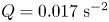 $Q=0.017\ \textrm {s}^{-2}$).

B.3. Wave structure
In order to show a wave structure in a boundary layer, a database obtained from the solution of nonlinear parabolized stability equations (NPSE) was used to reconstruct a time-line surface for a 3-D O-type transition wave (Jiang et al. Reference Jiang, Lee, Chen, Smith and Linden2020). A pair of oblique disturbances were introduced in the flow, causing the creation of 3-D waves, which amplified due to mode interaction as they travelled downstream. This O-type transition, shown in figure 30, is characterized by the appearance of LSSs. Note that a 3-D wave (W0) as it appears in the early stage of O-regime transition is identified in figure 30. The subsequent development of an LSS is observed to consist of several wave structures (W1, W2 and W3 in figure 30).
Time-lines reconstructed from NPSE database for O-type boundary layer transition (initiated at  $y \approx 50\,\%$
 $\delta$). LSS is within the white-dashed region, as indicated to the upper left of the figure.