1 Introduction
In recent years industrial design of subsonic jet engines has moved to consider less conventional nozzles, producing fully asymmetric three-dimensional flows for the benefit of noise control. Current rapid prediction methods, based on Lighthill’s acoustic analogy (Lighthill Reference Lighthill1952, Reference Lighthill1954), and that given by Lilley (Reference Lilley1958) for parallel shear flows, are restricted by their inability to incorporate flow–acoustic interaction effects as the jet deviates from the radially symmetric flow profiles generated by round nozzles. These effects, considered as the ‘finer details’ by Lighthill (Reference Lighthill1954), are now critical to noise prediction schemes.
Generalizations of the Lighthill acoustic analogy may be consistently formulated by linearizing the fluid dynamic equations of motion about a given arbitrary mean flow, retaining nonlinear perturbation terms as prescribed turbulence noise sources. The noise process is then decoupled into one of source generation and flow–acoustic interaction, where the latter relies on how accurately the mean flow describes the true time-averaged flow under consideration.
In the literature, one of the most popular methods of incorporating flow–acoustic interaction effects for arbitrary flows is to use the linearized Euler equations (see Goldstein Reference Goldstein1976). Solutions are then typically constructed by introducing a vector Green’s function, generated by a vector of point sources. The acoustic field is then calculated by convolving Green’s function with an appropriate space–time correlation of the turbulence source. The significance of this Green’s function for our purposes is that it perfectly encodes propagation effects for any localized source in an arbitrary jet and naturally lends itself as a means of extending Lighthill’s theory to encompass refraction (see Ribner Reference Ribner1995). In this paper, the determination of the Green’s function solution of the linearized Euler equations serves as our underlying aim, however, the solution technique demonstrated herein may then be readily extended to generalizations of these linear equations such as that due to Goldstein (Reference Goldstein2003).
Despite the simplicity in which we can formulate a convolution integral for the acoustic variables, calculation of Green’s function is still a major undertaking (see Tam & Pastouchenko Reference Tam and Pastouchenko2002). This is true even for the cases where the flow facilitates a reduction to a single wave equation, for example, a parallel shear flow in the case of Lilley (Reference Lilley1958). Therefore much attention has been focused on the simplifications gained by asymptotic limits of Green’s function in terms of wavenumber. The most fruitful of these, the high-frequency limit, arises when the acoustic wavelength is much shorter than the characteristic length scales of the mean flow. This approximation is certainly the case for noise emissions within a few jet diameters from the nozzle where the turbulence source intensity is highest.
In the high-frequency limit, acoustic propagation is described by ray theory, or geometric acoustics (see Pierce Reference Pierce1981). Ray theory has a successful history of combination with acoustic analogies as demonstrated by Balsa (Reference Balsa1976), Goldstein (Reference Goldstein1982), Durbin (Reference Durbin1983b ), Ilário et al. (Reference Ilário, Azarpeyvand, Rosa, Self and Meneghini2017), working to down to Helmholtz numbers of unity for total noise calculations (see Balsa Reference Balsa1976; Tester & Morfey Reference Tester and Morfey1976), and Strouhal numbers as low as a half for the accurate calculations of Green’s function (see Wundrow & Khavaran Reference Wundrow and Khavaran2004). Unlike Wundrow & Khavaran (Reference Wundrow and Khavaran2004), which focuses on a high-frequency modal solution, in our work we present a more general ray-based approach which contains several features not previously combined in the literature. We may summarize these in the following categories: the multiplicity of rays at a receiver point due to nonlinearity of the governing eikonal equation; the failure and prediction of unphysical divergences by rays at caustics; and unsuitable methods for the determination of complex rays, which model both exponentially growing and decaying waves. We show here that each of these problems are not only quantitatively significant, but also may be solved efficiently by reference to each of the others thus creating a computationally consistent and efficient ray programme.
The multiplicity problem arises from the trade-off between simplicity and nonlinearity made in the ray approximation. In the mean jet flows of interest, the nonlinear eikonal equation admits multiple, possibly complex, ray solutions, which describe space curves, or ray paths, connecting the acoustic point source and receiver locations (see Candel Reference Candel1977; Hanyga Reference Hanyga1996). Each ray solution depends continuously on initial data specified at the source, determining the ray endpoint once the ray equations are integrated. The difficulty lies in determining which sets of unique initial data values generate ray endpoints that lie at the receiver. As shown by Hanyga (Reference Hanyga1996), an appropriate way of circumventing this issue is by introducing a boundary value problem of which the required initial data values are the roots. This reformulation inherits the nonlinearity of the ray equations, but has merit in that it facilitates an optimization problem amenable to standard root-finding procedures. In this paper we tackle the optimization problem using a Newton-based iterative method as in Keller & Perozzi (Reference Keller and Perozzi1983), Keller (Reference Keller1992), that converges quadratically once an initial seed is provided. The method then generates multiple roots, or rays, as its outputs depending on the domain of convergence of the initial seed (see Allgower & Georg Reference Allgower and Georg1990).
When a receiver position coincides with a caustic, two or more roots of the boundary value problem coalesce, the corresponding ray solutions are then degenerate and the ray paths tangential. The envelope of degenerate rays forms a caustic surface, where the Jacobian of the rays is zero and the ray amplitude singular. While there are several alternative methods of providing uniformity at caustics, for example, using Gaussian beams (see Červený, Popov & Pšenčík Reference Červený, Popov and Pšenčík1982; Norris Reference Norris1986), here we use the uniform functions catastrophe theory (see Thom Reference Thom1989; Poston & Stewart Reference Poston and Stewart2014). This allows us to classify caustics in three dimensions as one of Thom’s seven stable catastrophes (see Berry & Upstill Reference Berry and Upstill1980; Olver et al. Reference Olver, Olde Daalhuis, Lozier, Schneider, Boisvert, Clark, Miller and Saunders2016, chap. 36), replacing singular rays by a locally valid asymptotic series in a canonical integral and its derivatives, that remains bounded at the caustic. Catastrophe theory is a natural choice for two reasons. First, the caustics of catastrophe theory are ubiquitous in high-frequency wave fields, structurally organizing the ray solution, making their features identifiable and straightforward to classify. Second, unknown quantities in the uniform formulae may be expressed in terms of the singular ray solutions at the caustic, with little additional computational effort.
In the above, both the roots and the caustic generating rays may be real or complex. Complex rays are extensions to the familiar real ray solutions, with the paths described by the ray equations lying on a surface in complexified space (see Chapman et al. Reference Chapman, Lawry, Ockendon and Tew1999). The complexification of rays facilitates the propagation of exponentially growing and decaying waves, the latter of which are critical for generating shadow zones, such as the cone of silence (see Goldstein Reference Goldstein1982; Stone, Howls & Self Reference Stone, Self and Howls2017; Hubbard Reference Goldstein1991, chap. 5), and as we show, capturing the finer details of oscillatory behaviour in the point source field. However, one cannot realistically perform global searches by seeding a Newton method with a complex ray, as is possible with real rays. This is due to the intricate behaviour of each complex root’s region of convergence. Instead one must find complex rays locally after an initial real ray search of the field.
In this paper, the key to local complex ray calculation is the presence of caustics described by catastrophe theory. As the boundary value problem roots bifurcate upon crossing the caustic, complex rays may be generated as the total number of real and complex rays must be conserved (see Berry & Upstill Reference Berry and Upstill1980). The complex rays may easily be latched onto as the imaginary parts of the complex roots are small. Local determination in this manner has the added benefit that exponentially small complex ray fields are at their largest near the caustic and therefore their inclusion there is the most significant. Alternatively, we show that one can bypass a caustic by taking a receiver position and detouring into complex space passing smoothly onto complex roots. If necessary the full set of coalescing rays may be checked for by looping the receiver around the caustic several times so that we fully explore the associated Riemann sheet structure. We then classify the caustic from the generating rays we pick up.
The mathematical basis for our ray solver, the linearized Euler equations and their vector Green’s function solution, is introduced in § 2. High-frequency ray solutions are then developed in § 3 where the eikonal and amplitude transport equations are solved using the characteristics of rays. In § 4 we formulate the boundary value problem for tackling ray multiplicity, using an equivalent Newton-based iteration to calculate the roots, combining solutions using a coherent ray sum. We then incorporate complex rays by applying a new splitting method to the ray equations in § 5. Complex continuation methods are presented in § 6 as a means of bypassing stable caustics, allowing for the local determination of complex rays. We then classify the caustic and correct for ray divergence by mapping the ray field to a local uniform catastrophe function in § 6.2. The ray solver is then demonstrated in §§ 7 and 8 for parallel shear and spreading jets respectively. In these sections we show that there is a striking self-similarity between the downstream regions of the high-frequency fields generated by point sources in both flows and that the upstream regions are organized about a newly observed cusp caustic.
2 Governing equations
The starting point for our calculations is the linearized system of inviscid Euler equations governing the propagation of acoustic disturbances through a prescribed mean flow (see Goldstein Reference Goldstein1976). For a time-harmonic disturbance with characteristic radian frequency of oscillation
 $\unicode[STIX]{x1D714}$
, these equations are given in Cartesian coordinates
 $\boldsymbol{x}=(x_{1},x_{2},x_{3})$
as
 $$\begin{eqnarray}\displaystyle & \displaystyle \bar{\unicode[STIX]{x1D70C}}\left(\overline{D}_{\unicode[STIX]{x1D714}}u_{i}^{\prime }+u_{j}^{\prime }\frac{\unicode[STIX]{x2202}\bar{u}_{i}}{\unicode[STIX]{x2202}x_{j}}\right)+\unicode[STIX]{x1D70C}^{\prime }\bar{u}_{j}\frac{\unicode[STIX]{x2202}\bar{u}_{i}}{\unicode[STIX]{x2202}x_{j}}+\frac{\unicode[STIX]{x2202}p^{\prime }}{\unicode[STIX]{x2202}x_{i}}={\mathcal{f}}_{i}, & \displaystyle\end{eqnarray}$$
 $$\begin{eqnarray}\displaystyle & \displaystyle \overline{D}_{\unicode[STIX]{x1D714}}\unicode[STIX]{x1D70C}^{\prime }+\unicode[STIX]{x1D70C}^{\prime }\frac{\unicode[STIX]{x2202}\bar{u}_{j}}{\unicode[STIX]{x2202}x_{j}}+\frac{\unicode[STIX]{x2202}}{\unicode[STIX]{x2202}x_{j}}\bar{\unicode[STIX]{x1D70C}}u_{j}^{\prime }=\bar{\unicode[STIX]{x1D70C}}{\mathcal{q}}, & \displaystyle\end{eqnarray}$$
 $$\begin{eqnarray}\displaystyle & \displaystyle \overline{D}_{\unicode[STIX]{x1D714}}s^{\prime }+u_{j}^{\prime }\frac{\unicode[STIX]{x2202}\bar{s}}{\unicode[STIX]{x2202}x_{j}}=0, & \displaystyle\end{eqnarray}$$
 $$\begin{eqnarray}\displaystyle & \displaystyle p^{\prime }-\bar{c}^{2}\unicode[STIX]{x1D70C}^{\prime }-\left(\frac{\overline{\unicode[STIX]{x2202}{\mathcal{k}}}}{\unicode[STIX]{x2202}s}\right)s^{\prime }=0, & \displaystyle\end{eqnarray}$$
where
 $p$
denotes the pressure,
 $\unicode[STIX]{x1D70C}$
denotes the density,
 $s$
denotes the entropy,
 $\boldsymbol{u}=(u_{1},u_{2},u_{3})$
denotes the velocity of the fluid,
 ${\mathcal{f}}$
and
 ${\mathcal{q}}$
are nonlinear volume sources,
 $p={\mathcal{k}}(\unicode[STIX]{x1D70C},s)$
defines the equation of state, which can be used to define the sound speed
 $c$
as below. Here we have used tensor notation with
 $i,j=1,2,3$
. In this paper repeated indices imply a tensor summation, unless stated otherwise.
Equations (2.1)–(2.4) describe the splitting of each dependent variable into mean and fluctuating parts, e.g.
 $\unicode[STIX]{x1D70C}=\bar{\unicode[STIX]{x1D70C}}+\unicode[STIX]{x1D70C}^{\prime }$
, so that a prime denotes an acoustic disturbance of
 $O(\unicode[STIX]{x1D716}),\unicode[STIX]{x1D716}\ll 1$
, and an overbar denotes a time average (see Goldstein Reference Goldstein1976),
 $$\begin{eqnarray}\bar{\bullet }\equiv \lim _{T\rightarrow +\infty }\frac{1}{2T}\int _{-T}^{T}\bullet (\boldsymbol{x},t)\,\text{d}t.\end{eqnarray}$$
The mean convective operator
 $\overline{D}_{\unicode[STIX]{x1D714}}$
is then defined by
 $$\begin{eqnarray}\overline{D}_{\unicode[STIX]{x1D714}}\equiv -\text{i}\unicode[STIX]{x1D714}+\bar{u}_{j}\frac{\unicode[STIX]{x2202}}{\unicode[STIX]{x2202}x_{j}}.\end{eqnarray}$$
We take the nonlinear volume sources
 $\boldsymbol{{\mathcal{f}}}=({\mathcal{f}}_{1},{\mathcal{f}}_{2},{\mathcal{f}}_{3})$
and
 ${\mathcal{q}}$
as
 $O(\unicode[STIX]{x1D716})$
, so both sides of (2.1)–(2.4) are commensurate in size. Both the mean variables and nonlinear volume sources are specified a priori, so that the acoustic variables are to be determined. The ambient values of all variables, i.e. outside of the jet
 ${\mathcal{f}}_{i},{\mathcal{q}},\bar{u}_{i}\rightarrow 0$
, are denoted by the subscript
 $\infty$
.
The equation of state is used to define the mean square sound speed
 $$\begin{eqnarray}\bar{c}^{2}\equiv \overline{\unicode[STIX]{x2202}{\mathcal{k}}}/\unicode[STIX]{x2202}\unicode[STIX]{x1D70C},\end{eqnarray}$$
which determines the mean sound speed profile explicitly in terms of a specified mean temperature profile via
 $$\begin{eqnarray}\bar{c}(\boldsymbol{x})=\sqrt{\unicode[STIX]{x1D6FE}R\bar{T}}.\end{eqnarray}$$
Here we have used the ideal gas law,
 $p=\unicode[STIX]{x1D70C}RT$
, and isentropic relation
 $p\propto \unicode[STIX]{x1D70C}^{\unicode[STIX]{x1D6FE}}$
for constant entropy, where
 $R$
denotes the gas constant,
 $\unicode[STIX]{x1D6FE}$
the heat capacity ratio and
 $T$
the absolute temperature. We then define the characteristic wavenumber
 $k_{0}$
using
 $k_{0}=\unicode[STIX]{x1D714}/\bar{c}_{\infty }$
.
The linearity of (2.1)–(2.4) suggests looking for a Green’s function solution so that the volume sources are decoupled from propagation. The vector Green’s function,
 $g_{\ell \unicode[STIX]{x1D702}}(\boldsymbol{x}|\boldsymbol{x}_{s})$
, of (2.1)–(2.4) satisfies (see Morse & Feshbach Reference Morse and Feshbach1953, pp. 878–886),
 $$\begin{eqnarray}\displaystyle & \displaystyle \bar{\unicode[STIX]{x1D70C}}\left(\overline{D}_{\unicode[STIX]{x1D714}}g_{i\unicode[STIX]{x1D702}}+g_{j\unicode[STIX]{x1D702}}\frac{\unicode[STIX]{x2202}\bar{u}_{i}}{\unicode[STIX]{x2202}x_{j}}\right)+g_{4\unicode[STIX]{x1D702}}\bar{u}_{j}\frac{\unicode[STIX]{x2202}\bar{u}_{i}}{\unicode[STIX]{x2202}x_{j}}+\frac{\unicode[STIX]{x2202}g_{5\unicode[STIX]{x1D702}}}{\unicode[STIX]{x2202}x_{i}}=\unicode[STIX]{x1D6FF}_{i\unicode[STIX]{x1D702}}\unicode[STIX]{x1D6FF}(\boldsymbol{x}-\boldsymbol{x}_{s}), & \displaystyle\end{eqnarray}$$
 $$\begin{eqnarray}\displaystyle & \displaystyle \overline{D}_{\unicode[STIX]{x1D714}}g_{4\unicode[STIX]{x1D702}}+g_{4\unicode[STIX]{x1D702}}\frac{\unicode[STIX]{x2202}\bar{u}_{j}}{\unicode[STIX]{x2202}x_{j}}+\frac{\unicode[STIX]{x2202}}{\unicode[STIX]{x2202}x_{j}}\bar{\unicode[STIX]{x1D70C}}g_{j\unicode[STIX]{x1D702}}=\unicode[STIX]{x1D6FF}_{4\unicode[STIX]{x1D702}}\unicode[STIX]{x1D6FF}(\boldsymbol{x}-\boldsymbol{x}_{s}), & \displaystyle\end{eqnarray}$$
 $$\begin{eqnarray}\displaystyle & \displaystyle \overline{D}_{\unicode[STIX]{x1D714}}g_{6\unicode[STIX]{x1D702}}+g_{j\unicode[STIX]{x1D702}}\frac{\unicode[STIX]{x2202}\bar{s}}{\unicode[STIX]{x2202}x_{j}}=0, & \displaystyle\end{eqnarray}$$
 $$\begin{eqnarray}\displaystyle & \displaystyle g_{5\unicode[STIX]{x1D702}}-\bar{c}^{2}g_{4\unicode[STIX]{x1D702}}-\left(\frac{\overline{\unicode[STIX]{x2202}{\mathcal{k}}}}{\unicode[STIX]{x2202}s}\right)g_{6\unicode[STIX]{x1D702}}=0, & \displaystyle\end{eqnarray}$$
where subscript
 $\ell =1,\ldots ,6$
, of
 $g_{\ell \unicode[STIX]{x1D702}}$
describes the response of the
 $\ell$
th acoustic variable of the vector
 $\boldsymbol{v}=(\boldsymbol{u}^{\prime },\unicode[STIX]{x1D70C}^{\prime },p^{\prime },s^{\prime })$
, to a point source forcing at
 $\boldsymbol{x}_{s}$
in the
 $\unicode[STIX]{x1D702}$
th equation (
 $\unicode[STIX]{x1D702}=1,\ldots ,4$
). Henceforth, subscript ‘
 $s$
’ is used to denote any quantity evaluated at the source point
 $\boldsymbol{x}_{s}$
.
Similarly to
 $\boldsymbol{v}$
, we define
 $\boldsymbol{Y}=(\boldsymbol{{\mathcal{f}}},{\mathcal{q}})$
with components
 $Y_{\unicode[STIX]{x1D702}}$
, as the volume source vector, so that we may write the solution to the frequency domain acoustic variables as the convolution
 $$\begin{eqnarray}v_{\ell }=\int _{V}g_{\ell \unicode[STIX]{x1D702}}(\boldsymbol{x}\mid \boldsymbol{x}_{s})Y_{\unicode[STIX]{x1D702}}(\boldsymbol{x}_{s})\,\text{d}\boldsymbol{x}_{s},\end{eqnarray}$$
over the source volume
 $V$
. Now, for example, the pressure component of
 $\boldsymbol{v}$
may then be computed by setting
 $\ell =5$
, requiring Green’s function components
 $g_{5\unicode[STIX]{x1D702}}$
.
3 High-frequency ray solutions
In the high-frequency limit (2.9)–(2.12) can be solved using ray theory. In free space there are two scenarios where this description is not valid locally: near caustics, which we discuss in § 6.2, and in the vicinity of a point source. In this section, we deal with the latter by constructing the high-frequency Green’s function as in Durbin (Reference Durbin1983a
). The formulation therein poses a ray ansatz for the homogeneous system of (2.9)–(2.12). This ‘outer’ solution is then matched to a solution valid near the source in the limit
 $\boldsymbol{x}\rightarrow \boldsymbol{x}_{s}$
(see Avila & Keller Reference Avila and Keller1963). It is implicit in this matching procedure that the overlap region, where these solutions are asymptotically equal, is free from any other singularities of the ray solution, which in free space means caustics.
We start by applying the ray ansatz to the homogeneous version of (2.9)–(2.12), i.e. setting the sources to zero, which we will match to the near source solution developed in appendix A. First, we drop any reference to
 $\unicode[STIX]{x1D702}$
that comes from the point source matrix
 $\unicode[STIX]{x1D6FF}_{\ell \unicode[STIX]{x1D702}}\unicode[STIX]{x1D6FF}(\boldsymbol{x}-\boldsymbol{x}_{s})$
, so that we primarily seek solutions
 $g_{\ell }$
, ultimately reattaching the index
 $\unicode[STIX]{x1D702}$
to find
 $g_{\ell \unicode[STIX]{x1D702}}$
via matching with the inner solution. In free space the ray solution is posed by an asymptotic ansatz ordered in integer powers of the wavenumber
 $k_{0}\rightarrow +\infty$
,
 $$\begin{eqnarray}g_{\ell }\sim \text{e}^{\text{i}k_{0}S}\mathop{\sum }_{n=0}^{\infty }\frac{A_{\ell n}}{(\text{i}k_{0})^{n}},\quad A_{\ell n}=(\bar{c}_{\infty }\boldsymbol{m}_{n},r_{n},P_{n},s_{n}),\end{eqnarray}$$
where
 $S$
is the phase of the ray and
 $A_{\ell n}$
is the
 $n$
th amplitude term of the series, a placeholder for each physical variable ordered according to
 $\boldsymbol{v}$
of (2.13), i.e. for
 $\ell =1,2,3$
,
 $\boldsymbol{m}_{n}$
denotes acoustic velocity;
 $\ell =4$
,
 $r_{n}$
denotes the density;
 $\ell =5$
,
 $P_{n}$
denotes the pressure;
 $\ell =6$
,
 $s_{n}$
denotes the entropy.
The independence of the outer ray solution upon
 $\unicode[STIX]{x1D702}$
means we may follow the mechanics of Jones (Reference Jones1976) in constructing a solution along with Durbin (Reference Durbin1983a
). The following provides an outline of the key results from those papers.
The ansatz (3.1) is formally introduced into the homogeneous form of (2.9)–(2.12) once
 $k_{0}$
is made explicit via
 $\overline{D}_{\unicode[STIX]{x1D714}}$
. This leads to a sequence of coupled equations in
 $S$
and
 $A_{\ell n}$
of which we only need the first two for asymptotic numerical calculations: the eikonal equation governing
 $S$
and transport equation governing
 $A_{\ell 0}$
(the first amplitude term in (3.1)).
The eikonal equation is a first-order nonlinear partial differential equation in spatial derivatives of
 $S$
. Defining the slowness vector
 $\boldsymbol{p}\equiv (\unicode[STIX]{x2202}S/\unicode[STIX]{x2202}x_{1},\unicode[STIX]{x2202}S/\unicode[STIX]{x2202}x_{2},\unicode[STIX]{x2202}S/\unicode[STIX]{x2202}x_{3})$
, as proportional to the wavefront normal
 $\boldsymbol{n}$
,
 $\boldsymbol{M}(\boldsymbol{x})\equiv \bar{\boldsymbol{u}}(\boldsymbol{x})/\bar{c}_{\infty }$
as the acoustic Mach number vector and
 $a(\boldsymbol{x})\equiv \bar{c}(\boldsymbol{x})/\bar{c}_{\infty }$
as the sound speed ratio. The eikonal equation is then given by
 $$\begin{eqnarray}a^{-2}(1-\boldsymbol{M}\boldsymbol{\cdot }\boldsymbol{p})^{2}-\boldsymbol{p}\boldsymbol{\cdot }\boldsymbol{p}=\boldsymbol{p}\boldsymbol{\cdot }\unicode[STIX]{x1D64F}\boldsymbol{\cdot }\boldsymbol{p}+2\boldsymbol{M}\boldsymbol{\cdot }\boldsymbol{p}/a-1/a^{2}=0,\end{eqnarray}$$
in terms of the matrix
 $\unicode[STIX]{x1D64F}$
 $$\begin{eqnarray}\unicode[STIX]{x1D64F}=\unicode[STIX]{x1D644}-\boldsymbol{M}\otimes \boldsymbol{M}/a^{2},\quad \unicode[STIX]{x1D64F}^{-1}=\unicode[STIX]{x1D644}+\boldsymbol{M}\otimes \boldsymbol{M}/\unicode[STIX]{x1D6FD}^{2}a^{2},\quad \unicode[STIX]{x1D6FD}^{2}=1-\boldsymbol{M}\boldsymbol{\cdot }\boldsymbol{M}/a^{2},\end{eqnarray}$$
where
 $\otimes$
is an outer product and
 $\unicode[STIX]{x1D644}$
the unit matrix.
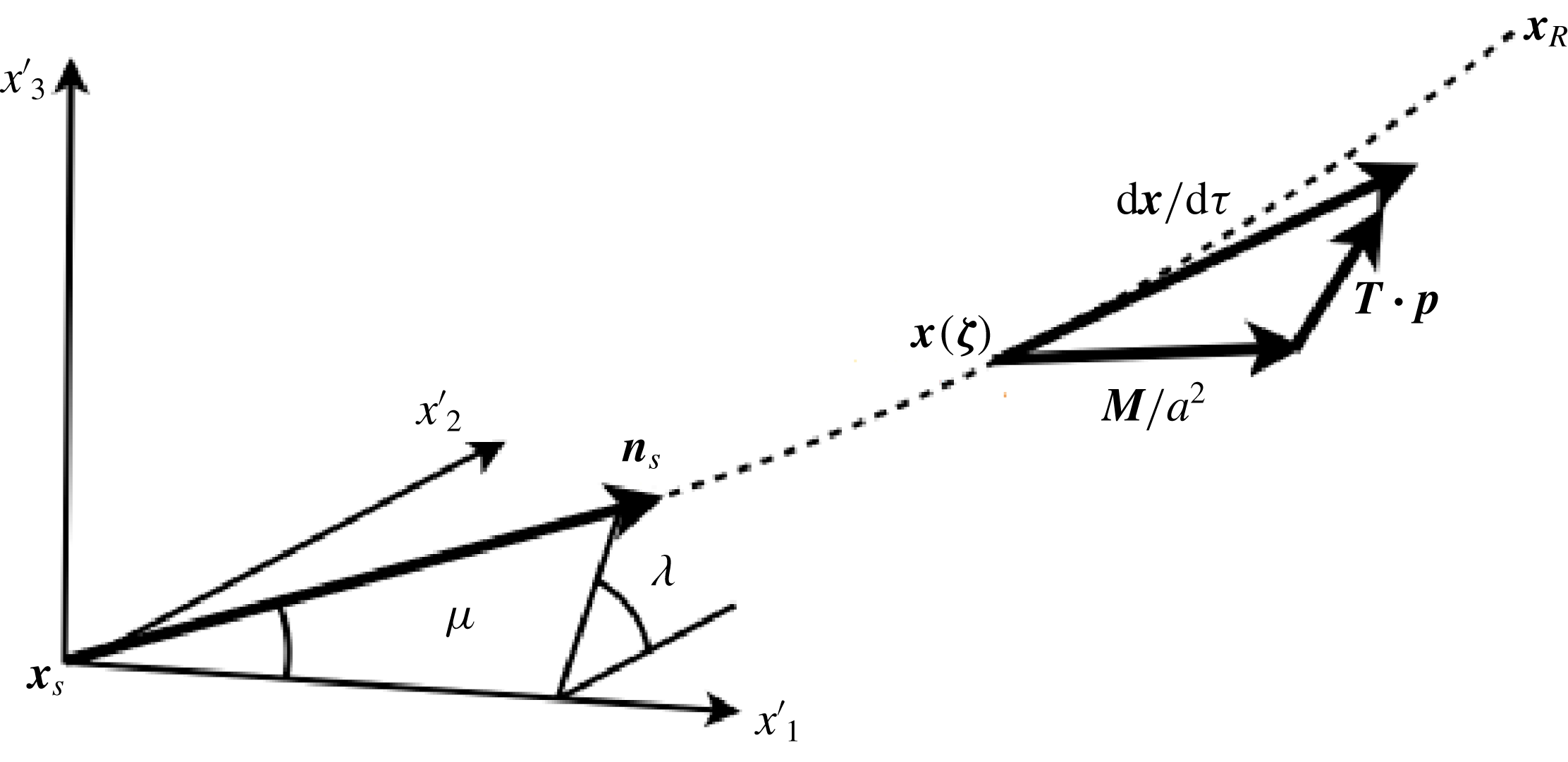
Ray initial values for propagating ray
 $\boldsymbol{x}(\unicode[STIX]{x1D73B})$
(dashed line) from source
 $\boldsymbol{x}_{s}$
to receiver
 $\boldsymbol{x}_{R}$
where
 $\boldsymbol{x}^{\prime }=\boldsymbol{x}-\boldsymbol{x}_{s}$
, are local source coordinates,
 $\unicode[STIX]{x1D707}$
polar and
 $\unicode[STIX]{x1D706}$
azimuthal angles generate initial normal
 $\boldsymbol{n}_{s}$
. Local velocity triangle in
 $\text{d}\boldsymbol{x}/\text{d}\unicode[STIX]{x1D70F}$
,
 $\boldsymbol{M}/a^{2}$
,
 $\unicode[STIX]{x1D64F}\boldsymbol{\cdot }\boldsymbol{p}$
, is the geometric interpretation of (3.4).

The eikonal equation may be solved using the method of characteristics (see Sneddon Reference Sneddon2006). The phase,
 $S$
, of the ray ansatz (3.1) is then propagated along the characteristics, or rays, from the source
 $\boldsymbol{x}_{s}$
to the receiver
 $\boldsymbol{x}_{R}$
. Although the full ray solution of (3.1) must be matched to the inner solution of appendix A to be determined fully, the phase,
 $S$
, may be initialized using rays without reference to the matching procedure.
The initial data require three ray parameters,
 $\unicode[STIX]{x1D73B}=(\unicode[STIX]{x1D707},\unicode[STIX]{x1D706},\unicode[STIX]{x1D70F}_{e})$
, where
 $\unicode[STIX]{x1D707}$
and
 $\unicode[STIX]{x1D706}$
are polar and azimuthal angles orienting the ray direction, as shown in figure 1, and
 $\unicode[STIX]{x1D70F}_{e}$
the integration time along the ray. The ray equations, which are nonlinear ordinary differential equations governing the position
 $\boldsymbol{x}(\unicode[STIX]{x1D73B})$
, slowness
 $\boldsymbol{p}$
, and phase
 $S$
, are given by the initial value problem
 $$\begin{eqnarray}\displaystyle & \displaystyle \frac{\text{d}x_{i}}{\text{d}\unicode[STIX]{x1D70F}}=\unicode[STIX]{x1D61B}_{ij}(\boldsymbol{x})p_{j}+\frac{M_{i}(\boldsymbol{x})}{a^{2}(\boldsymbol{x})}, & \displaystyle\end{eqnarray}$$
 $$\begin{eqnarray}\displaystyle & \displaystyle \frac{\text{d}p_{i}}{\text{d}\unicode[STIX]{x1D70F}}=-\frac{1}{2}p_{j}\frac{\unicode[STIX]{x2202}\unicode[STIX]{x1D61B}_{jm}(\boldsymbol{x})}{\unicode[STIX]{x2202}x_{i}}p_{m}-p_{j}\frac{\unicode[STIX]{x2202}}{\unicode[STIX]{x2202}x_{i}}\left(\frac{M_{j}(\boldsymbol{x})}{a^{2}(\boldsymbol{x})}\right)+\frac{1}{2}\frac{\unicode[STIX]{x2202}a^{-2}(\boldsymbol{x})}{\unicode[STIX]{x2202}x_{i}}, & \displaystyle\end{eqnarray}$$
 $$\begin{eqnarray}\displaystyle & \displaystyle \frac{\text{d}S}{\text{d}\unicode[STIX]{x1D70F}}=p_{j}\frac{\text{d}x_{j}}{\text{d}\unicode[STIX]{x1D70F}}, & \displaystyle\end{eqnarray}$$
where
 $i,j,m=1,2,3$
, and initial conditions at
 $\unicode[STIX]{x1D70F}=0$
(see Durbin Reference Durbin1983a
),
 $$\begin{eqnarray}\displaystyle x_{i}(0)=x_{s_{i}},\quad p_{i}(0)=\unicode[STIX]{x1D61B}_{s_{ij}}^{-1}(\unicode[STIX]{x1D70E}_{s}n_{s_{j}}-M_{s_{j}}/a_{s}^{2}),\quad S(0)=0,\quad \unicode[STIX]{x1D70E}_{s}^{-2}=(n_{s_{i}}\unicode[STIX]{x1D61B}_{s_{ij}}^{-1}n_{s_{j}})a_{s}^{2}\unicode[STIX]{x1D6FD}_{s}^{2}. & & \displaystyle \nonumber\\ \displaystyle & & \displaystyle\end{eqnarray}$$
Here the initial firing direction
 $\boldsymbol{n}_{s}=(\cos \unicode[STIX]{x1D707},\sin \unicode[STIX]{x1D707}\cos \unicode[STIX]{x1D706},\sin \unicode[STIX]{x1D707}\sin \unicode[STIX]{x1D706})$
, as shown in figure 1, is chosen to be proportional to the initial ray group velocity
 $\text{d}\boldsymbol{x}/\text{d}\unicode[STIX]{x1D70F}=\unicode[STIX]{x1D70E}_{s}\boldsymbol{n}_{s}$
, where
 $\unicode[STIX]{x1D70E}=|\text{d}\boldsymbol{x}/\text{d}\unicode[STIX]{x1D70F}|$
is the ray speed. The equations may be integrated once the mean flow profiles are specified.
3.1 Ray amplitude
In this section we outline the solution of the ray amplitude, starting from the divergence form of the transport equation given by Jones (Reference Jones1976) and Durbin (Reference Durbin1983a ). An exact solution of the transport equation requires an extension of the ray equations (3.4)–(3.6), which we derive below.
The divergence form of the transport equation is given in terms of the density amplitude
 $r_{0}$
(i.e.
 $A_{\ell 0}$
, with
 $\ell =4$
) and is stated as
 $$\begin{eqnarray}\frac{\unicode[STIX]{x2202}}{\unicode[STIX]{x2202}x_{i}}\left[\frac{a^{4}r_{0}^{2}}{\bar{\unicode[STIX]{x1D70C}}(1-\boldsymbol{M}\boldsymbol{\cdot }\boldsymbol{p})^{2}}\frac{\text{d}x_{i}}{\text{d}\unicode[STIX]{x1D70F}}\right]=0,\quad i=1,2,3.\end{eqnarray}$$
Implicit in this equation is the important result that the eikonal equation represents acoustic disturbances. As shown in Jones (Reference Jones1976) this results in the requirement that the high-frequency wave is isentropic to leading order, i.e.
 $s_{0}=0$
(cf. (3.1)). The isentropic relation
 $P_{0}=\bar{c}^{2}r_{0}$
is then implied by (2.12), which may be used to express (3.8) in terms of pressure amplitude.
Equation (3.8) is solved by integrating over a hypothetical ray tube of vanishing area (see Durbin Reference Durbin1983a ) to give
 $$\begin{eqnarray}\unicode[STIX]{x1D6E9}=\frac{\unicode[STIX]{x1D70E}a^{4}P_{0}^{2}J}{\bar{\unicode[STIX]{x1D70C}}\bar{c}^{4}(1-\boldsymbol{M}\boldsymbol{\cdot }\boldsymbol{p})^{2}},\end{eqnarray}$$
where
 $\unicode[STIX]{x1D6E9}$
is a constant along the ray to be determined by matching at the source and
 $J$
is the Jacobian along the ray defined as the determinant of the Jacobian matrix (see Hayes Reference Hayes1970),
 $$\begin{eqnarray}\unicode[STIX]{x1D645}\equiv \left[\frac{\unicode[STIX]{x2202}\boldsymbol{x}}{\unicode[STIX]{x2202}\unicode[STIX]{x1D73B}}\right],\quad J\equiv \text{det}(\unicode[STIX]{x1D645}).\end{eqnarray}$$
Equation (3.9) may then be inverted to find
 $P_{0}$
and all other leading-order acoustic variable amplitudes using either the isentropic relation or
 $$\begin{eqnarray}\boldsymbol{m}_{0}=\frac{a^{2}r_{0}\boldsymbol{p}}{\bar{\unicode[STIX]{x1D70C}}(1-\boldsymbol{M}\boldsymbol{\cdot }\boldsymbol{p})},\end{eqnarray}$$
which relates acoustic velocity to density as shown in Jones (Reference Jones1976).
Now, the only quantity that varies along a ray that is not accounted for in (3.9) is the Jacobian,
 $J$
. The Jacobian requires the calculation of the geodesic elements
 $y_{ik}=\unicode[STIX]{x2202}x_{i}/\unicode[STIX]{x2202}\unicode[STIX]{x1D701}_{k}$
,
 $i,k=1,2,3$
, that necessitate an additional set of derived equations (see Hayes Reference Hayes1970; Candel Reference Candel1977). These equations are generated by differentiating (3.4) and (3.5) with respect to
 $(\tilde{\unicode[STIX]{x1D707}}_{1},\tilde{\unicode[STIX]{x1D707}}_{2})=(\unicode[STIX]{x1D707},\unicode[STIX]{x1D706})$
, thereby introducing the coupled conjugate elements,
 $z_{ik}=\unicode[STIX]{x2202}p_{i}/\unicode[STIX]{x2202}\unicode[STIX]{x1D701}_{k}$
. We note that no additional equations are required for the elements
 $y_{i3}=\unicode[STIX]{x2202}x_{i}/\unicode[STIX]{x2202}\unicode[STIX]{x1D70F}$
and
 $z_{i3}=\unicode[STIX]{x2202}p_{i}/\unicode[STIX]{x2202}\unicode[STIX]{x1D70F}$
,
 $\forall i$
, as these reduce to ordinary differentiation along the ray and are given by (3.4) and (3.5), respectively.
Differentiation is facilitated by the commutative relations for time-harmonic rays in free space (cf. Hayes Reference Hayes1970),
 $$\begin{eqnarray}\frac{\unicode[STIX]{x2202}}{\unicode[STIX]{x2202}\tilde{\unicode[STIX]{x1D707}}_{k}}\frac{\text{d}x_{i}}{\text{d}\unicode[STIX]{x1D70F}}=\frac{\text{d}}{\text{d}\unicode[STIX]{x1D70F}}\frac{\unicode[STIX]{x2202}x_{i}}{\unicode[STIX]{x2202}\tilde{\unicode[STIX]{x1D707}}_{k}},\quad \frac{\unicode[STIX]{x2202}}{\unicode[STIX]{x2202}\tilde{\unicode[STIX]{x1D707}}_{k}}\frac{\text{d}p_{i}}{\text{d}\unicode[STIX]{x1D70F}}=\frac{\text{d}}{\text{d}\unicode[STIX]{x1D70F}}\frac{\unicode[STIX]{x2202}p_{i}}{\unicode[STIX]{x2202}\tilde{\unicode[STIX]{x1D707}}_{k}},\quad k=1,2,\end{eqnarray}$$
so that the derived ray equations are then determined as
 $$\begin{eqnarray}\frac{\text{d}y_{ik}}{\text{d}\unicode[STIX]{x1D70F}}=[(\unicode[STIX]{x2202}_{h}\unicode[STIX]{x1D61B}_{ij}(\boldsymbol{x})p_{j})+\unicode[STIX]{x2202}_{h}(M_{i}(\boldsymbol{x})/a^{2}(\boldsymbol{x}))]y_{hk}+\unicode[STIX]{x1D61B}_{ij}(\boldsymbol{x})z_{jk},\end{eqnarray}$$
 $$\begin{eqnarray}\displaystyle \frac{\text{d}z_{ik}}{\text{d}\unicode[STIX]{x1D70F}} & = & \displaystyle \left[-\frac{1}{2}p_{j}(\unicode[STIX]{x2202}_{h}\unicode[STIX]{x2202}_{i}\unicode[STIX]{x1D61B}_{jm}(\boldsymbol{x}))p_{m}-p_{j}\unicode[STIX]{x2202}_{h}\unicode[STIX]{x2202}_{i}(M_{j}(\boldsymbol{x})/a^{2}(\boldsymbol{x}))+\frac{1}{2}\unicode[STIX]{x2202}_{h}\unicode[STIX]{x2202}_{i}(a^{-2}(\boldsymbol{x}))\right]y_{hk}\nonumber\\ \displaystyle & & \displaystyle -\,[(\unicode[STIX]{x2202}_{i}\unicode[STIX]{x1D61B}_{jm}(\boldsymbol{x}))p_{m}+\unicode[STIX]{x2202}_{i}(M_{j}(\boldsymbol{x})/a^{2}(\boldsymbol{x}))]z_{jk},\end{eqnarray}$$
where
 $h=1,2,3$
,
 $k=1,2$
and for convenience
 $\unicode[STIX]{x2202}_{i}\equiv \unicode[STIX]{x2202}/\unicode[STIX]{x2202}x_{i}$
.
The initial conditions are determined in a similar manner, by differentiating (3.7) with respect to
 $\tilde{\unicode[STIX]{x1D741}}$
:
 $$\begin{eqnarray}y_{ik}(0)=0,\quad \forall i,k,\end{eqnarray}$$
 $$\begin{eqnarray}\displaystyle z_{ik}(0) & = & \displaystyle \frac{\unicode[STIX]{x2202}\unicode[STIX]{x1D70E}_{s}}{\unicode[STIX]{x2202}\tilde{\unicode[STIX]{x1D707}}_{k}}\unicode[STIX]{x1D61B}_{s_{ij}}^{-1}n_{s_{j}}+\unicode[STIX]{x1D70E}_{s}\unicode[STIX]{x1D61B}_{s_{ij}}^{-1}\frac{\unicode[STIX]{x2202}n_{s_{j}}}{\unicode[STIX]{x2202}\tilde{\unicode[STIX]{x1D707}}_{k}}\nonumber\\ \displaystyle & = & \displaystyle \unicode[STIX]{x1D70E}_{s}^{3}\left(M_{s_{j}}\frac{\unicode[STIX]{x2202}n_{s_{j}}}{\unicode[STIX]{x2202}\tilde{\unicode[STIX]{x1D707}}_{k}}\right)[M_{s_{i}}-(n_{s_{k}}M_{s_{k}})n_{s_{i}}]+\unicode[STIX]{x1D70E}_{s}\frac{\unicode[STIX]{x2202}n_{s_{i}}}{\unicode[STIX]{x2202}\tilde{\unicode[STIX]{x1D707}}_{k}},\end{eqnarray}$$
where the first set of conditions
 $y_{ik}=0$
derives from the independence of the source point
 $\boldsymbol{x}_{s}$
of ray parameters. This also confirms
 $\boldsymbol{x}_{s}$
as a singularity of Green’s function so that
 $J\rightarrow 0$
as
 $\boldsymbol{x}\rightarrow \boldsymbol{x}_{s}$
(see Avila & Keller Reference Avila and Keller1963).
We may now complete the leading-order ray solution by substituting in the constant
 $\unicode[STIX]{x1D6E9}$
of (3.9) determined in (A 6). This shows the leading-order behaviour of each ray contribution to the approximation of
 $g_{5\unicode[STIX]{x1D702}}$
is then given by
 $$\begin{eqnarray}{\mathcal{A}}_{\unicode[STIX]{x1D702}}a_{s}\frac{(1-\boldsymbol{M}\boldsymbol{\cdot }\boldsymbol{p})}{(1-\boldsymbol{M}_{s}\boldsymbol{\cdot }\boldsymbol{p}_{s})}\left(\frac{\bar{\unicode[STIX]{x1D70C}}\unicode[STIX]{x1D70E}_{s}^{3}\sin \unicode[STIX]{x1D707}}{\bar{\unicode[STIX]{x1D70C}}_{s}\unicode[STIX]{x1D70E}J}\right)^{1/2}\frac{\text{e}^{\text{i}k_{0}S}}{4\unicode[STIX]{x03C0}},\end{eqnarray}$$
where
 ${\mathcal{A}}_{\unicode[STIX]{x1D702}}$
is the algebraic operator defined in (A 2) and a function of ray parameters at source, e.g.
 $\boldsymbol{p}_{s}$
. The total field will be a sum of such solutions. All other
 $g_{\ell \unicode[STIX]{x1D702}}$
may be determined using the relationships between the various amplitudes
 $A_{\ell 0}$
, i.e.
 $s_{0}=0$
,
 $P_{0}=\bar{c}^{2}r_{0}$
, the isentropic conditions, and (3.11).
4 Boundary value problem
The initial value problem of (3.4)–(3.6) is a function of ray parameters,
 $\unicode[STIX]{x1D73B}$
, implicitly and not the desired receiver point, which is henceforth denoted as
 $\boldsymbol{x}_{R}$
. Thereby we have no means of determining those parameters,
 $\unicode[STIX]{x1D73B}=(\unicode[STIX]{x1D707},\unicode[STIX]{x1D706},\unicode[STIX]{x1D70F}_{e})$
, for which the ray end satisfies
 $\boldsymbol{x}(\unicode[STIX]{x1D73B})=\boldsymbol{x}_{R}$
. One way of inverting this relationship is by forming a boundary value problem as the difference between the ray end
 $\boldsymbol{x}(\unicode[STIX]{x1D73B})$
and the receiver position
 $\boldsymbol{x}_{R}$
(see Pereyra, Lee & Keller Reference Pereyra, Lee and Keller1980; Sambridge & Kennett Reference Sambridge and Kennett1990; Hanyga Reference Hanyga1996),
 $$\begin{eqnarray}\boldsymbol{F}(\unicode[STIX]{x1D73B};\boldsymbol{x}_{R})\equiv \boldsymbol{x}(\unicode[STIX]{x1D73B})-\boldsymbol{x}_{R},\end{eqnarray}$$
so that rays passing through the two endpoints,
 $\boldsymbol{x}_{s}$
and
 $\boldsymbol{x}_{R}$
, will have ray parameters,
 $\unicode[STIX]{x1D73B}_{\star }=(\unicode[STIX]{x1D707}_{\star },\unicode[STIX]{x1D706}_{\star },\unicode[STIX]{x1D70F}_{\star })$
, satisfying
 $$\begin{eqnarray}\boldsymbol{F}(\unicode[STIX]{x1D73B}_{\star };\boldsymbol{x}_{R})=\mathbf{0}.\end{eqnarray}$$
In general (4.1) is only soluble by quadrature and is non-trivial to invert to find
 $\unicode[STIX]{x1D73B}_{\star }(\boldsymbol{x}_{R})$
. Here we use an equivalent iterative scheme based on a multi-dimensional Newton method as in Keller (Reference Keller1992),
 $$\begin{eqnarray}\unicode[STIX]{x1D73B}^{(w+1)}=\unicode[STIX]{x1D73B}^{(w)}-[D\boldsymbol{F}^{+}(\unicode[STIX]{x1D73B}^{(w)};\boldsymbol{x}_{R})]\boldsymbol{F}(\unicode[STIX]{x1D73B}^{(w)};\boldsymbol{x}_{R}),\end{eqnarray}$$
where
 $w=0,1,2,\ldots ,$
is an iterative counter,
 $D\boldsymbol{F}$
is the transpose of
 $\unicode[STIX]{x1D645}$
defined in (3.10), and superscript
 $+$
denotes a pseudoinverse.
The boundary value problem (4.1) is inherently nonlinear and admits multiple solutions,
 $\unicode[STIX]{x1D73B}_{\star }$
, corresponding to multiple distinct rays. In order to generate a full solution to the ray field we apply the algorithm outlined in Amodei et al. (Reference Amodei, Keers, Vasco and Johnson2006). The algorithm starts by locating as many real rays as possible that propagate to the receiver point,
 $\boldsymbol{x}_{R}$
. First, a distribution of real initial ray parameter seeds,
 $\unicode[STIX]{x1D73B}^{(0)}$
, are used to calculate the ray trajectories, endpoints and geodesic elements required in (4.1), (4.3). The ray parameters are then updated using (4.3) and the procedure of calculating each ray repeated until convergence is detected by
 $\boldsymbol{x}(\unicode[STIX]{x1D73B})\approx \boldsymbol{x}_{R}$
. Here convergence is detected when the Euclidean norm
 $\Vert \boldsymbol{F}\Vert _{2}\ll 1$
. Those solutions reaching
 $\boldsymbol{x}_{R}$
that are not unique, for instance rays that reproduce another solution by generating the same initial normal
 $\boldsymbol{n}_{s}$
, are discarded. If no real ray solutions are found, the receiver position lies in a shadow zone, and
 $\boldsymbol{x}_{R}$
is moved towards the upstream region of the jet until at least one real ray is found.
Equation (4.3) is valid for complex rays as well given a suitable complex ray parameter,
 $\unicode[STIX]{x1D73B}^{(0)}$
, however, these initial seeds are very difficult to find using the global search method advocated above. An alternative local method is considered in § 6.1, once we have extended the ray-tracing integration to complex trajectories as in § 5.
The set of unique solutions, or family of rays, determined at a particular receiver point may then be used to seed (4.3) for a nearby receiver point. The family of rays may then be tracked along a receiver curve,
 $\boldsymbol{x}_{R}(\unicode[STIX]{x1D6FC})$
, when controlled by a parametric dependence on a scalar,
 $\unicode[STIX]{x1D6FC}$
. The multiple solutions of (4.2) corresponding to this family create smooth solution branches in the parameters
 $\unicode[STIX]{x1D73B}_{\star }$
. These branches are distinct, except at caustics where they coalesce and subsequently bifurcate (Allgower & Georg Reference Allgower and Georg1990). We consider this case in § 6.
When the receiver
 $\boldsymbol{x}_{R}$
lies away from caustics we may sum the
 $N$
(possibly complex) ray field contributions corresponding to
 $N$
distinct roots,
 $(\unicode[STIX]{x1D73B}_{\star _{1}},\ldots ,\unicode[STIX]{x1D73B}_{\star _{N}})$
, of (4.3) using a coherent superposition of solutions (3.17). For the pressure Green’s function components this gives
 $$\begin{eqnarray}g_{5\unicode[STIX]{x1D702}}\sim \mathop{\sum }_{n_{r}=1}^{N}{\mathcal{A}}_{\unicode[STIX]{x1D702}}^{(n_{r})}P_{0}^{(n_{r})}\text{e}^{\text{i}k_{0}S^{(n_{r})}}.\end{eqnarray}$$
The complex rays included in (4.4) are always exponentially decaying so that
 $g_{5\unicode[STIX]{x1D702}}$
does not grow unphysically as
 $k_{0}\rightarrow +\infty$
.
5 Complex ray tracing
In the previous section multiple rays are determined at
 $\boldsymbol{x}_{R}$
by considering an equivalent boundary value problem (4.2). In order to accommodate complex rays in this problem, we pose a more suitable ray integration procedure.
Complex rays are propagated from a real source to any observer
 $\boldsymbol{x}_{R}$
using complex parameters,
 $\unicode[STIX]{x1D73B}=(\unicode[STIX]{x1D707},\unicode[STIX]{x1D706},\unicode[STIX]{x1D70F}_{e})$
. The integration path is then not constrained to lie in real space. We may facilitate this by splitting each variable and ray equation, (3.4)–(3.6) and (3.13)–(3.14), into real and imaginary parts. Then we parameterize the integration path between
 $\unicode[STIX]{x1D70F}=0$
and a specific endpoint,
 $\unicode[STIX]{x1D70F}_{e}\in \mathbb{C}$
, as a function of the monotonically increasing real parameter
 $s_{\unicode[STIX]{x1D70F}}\in [0,1]$
where
 $s_{\unicode[STIX]{x1D70F}}=0$
and
 $s_{\unicode[STIX]{x1D70F}}=1$
correspond to the source and observer points, respectively. A straight line in the complex plane between
 $\unicode[STIX]{x1D70F}=0$
and
 $\unicode[STIX]{x1D70F}_{e}$
, has parameterization
 $\unicode[STIX]{x1D70F}=s_{\unicode[STIX]{x1D70F}}\unicode[STIX]{x1D70F}_{e}$
. The result as shown below is a system double in size, but with integrations still along the real line in
 $s_{\unicode[STIX]{x1D70F}}$
.
Each component of the ray initial value problems, (3.4)–(3.6) and (3.13)–(3.14), takes the form
 $$\begin{eqnarray}\frac{\text{d}f}{\text{d}\unicode[STIX]{x1D70F}}=F(\boldsymbol{f},\unicode[STIX]{x1D70F}),\quad f(0)=f_{0},\end{eqnarray}$$
where
 $f$
is one particular ray variable of all the others,
 $\boldsymbol{f}$
, coupled together in a given function
 $F$
with initial conditions
 $f_{0}$
. The splitting of
 $f$
into real and imaginary parts,
 $f=f_{\text{R}}+\text{i}f_{\text{I}}$
, results in
 $$\begin{eqnarray}\displaystyle \left.\begin{array}{@{}c@{}}\displaystyle \frac{\text{d}}{\text{d}s_{\unicode[STIX]{x1D70F}}}\left[\begin{array}{@{}c@{}}f_{R}\\ f_{I}\end{array}\right]=\left[\begin{array}{@{}c@{}}\text{Re}(\unicode[STIX]{x1D70F}_{e})\\ \text{Im}(\unicode[STIX]{x1D70F}_{e})\end{array}\right]\text{Re}(F(\boldsymbol{f},\unicode[STIX]{x1D70F}))\mp \left[\begin{array}{@{}c@{}}\text{Im}(\unicode[STIX]{x1D70F}_{e})\\ \text{Re}(\unicode[STIX]{x1D70F}_{e})\end{array}\right]\text{Im}(F(\boldsymbol{f},\unicode[STIX]{x1D70F})),\\ f_{R}(0)=\text{Re}(f_{0}),\quad f_{I}(0)=\text{Im}(f_{0}),\end{array}\right\} & & \displaystyle\end{eqnarray}$$
where the chain rule has been employed to transfer differentiation from
 $\unicode[STIX]{x1D70F}$
to
 $s_{\unicode[STIX]{x1D70F}}$
, and
 $\mp$
is negative for
 $f_{R}$
and positive for
 $f_{I}$
components.
In this work we follow a straight line integration path, however, it is possible to integrate along any piecewise smooth path joining the integration endpoints provided that no singularities obstruct the path of deformation.
6 Bifurcations, caustics and catastrophes
While (4.3) and (4.4) remain valid for regular field points, the former encounters bifurcations at caustics, while the latter must be amended for divergence in a neighbourhood containing a caustic as the Jacobian,
 $J$
, defined in (3.10) tends to zero. Here we have chosen to tackle both simultaneously using catastrophe theory. A key reason is that catastrophe theory not only describes the geometric forms of caustics, but also the integrals which describe the uniform field near caustics.
6.1 Continuation method
The branches of solutions in
 $\unicode[STIX]{x1D73B}_{\star }$
, that correspond to singular ray solutions and tangent ray paths, bifurcate at a caustic. We can then no longer use (4.3) with impunity, but must take care to address the rapid, and possibly complex, jumps in these ray parameters. Here we deal with caustics by adding a perturbation technique and complex continuation to the tracking algorithm of the previous section.
First, the algorithm tracks the family of rays with real ray parameters as detailed in § 4. According to the principle of ray conservation, the total number of rays in the family should remain constant as the receiver curve is traversed (see Berry & Upstill Reference Berry and Upstill1980). When a caustic is encountered a number of the singular rays will transition to complex parameters generating complex rays, with the remainder continued using the regularity provided by the pseudoinverse in (4.3). Without using complex ray tracing these rays would then be lost and the number of rays reduced. This reduction is detected and an imaginary perturbation is added to the last recorded values of the disappearing parameters
 $\unicode[STIX]{x1D73B}_{\star }$
as the next input into (4.3). The algorithm then latches on to complex rays in local manner at caustics tracking these solutions along the remainder of the receiver curve.
An alternative is to bypass the caustic completely by complexifiying the receiver coordinates
 $\boldsymbol{x}_{R}$
via
 $\unicode[STIX]{x1D6FC}$
. For example, near to
 $\unicode[STIX]{x1D6FC}_{C}$
, which denotes the parameter value for which the caustic is intersected, we then use
 $\unicode[STIX]{x1D6FC}=\unicode[STIX]{x1D6FC}_{C}+\bar{\unicode[STIX]{x1D6FC}}\exp (\text{i}v)$
to loop about the caustic arriving on the other side of
 $\unicode[STIX]{x1D6FC}_{C}$
, where
 $\bar{\unicode[STIX]{x1D6FC}}$
is the radius of the loop, and
 $v$
is a phase whose values determine which direction
 $\boldsymbol{x}_{R}$
is traversed (e.g.
 $0$
to
 $\unicode[STIX]{x03C0}$
, or
 $\unicode[STIX]{x03C0}$
to
 $0$
). This has two particular advantages to the perturbation technique. First, no perturbation is required to latch onto complex rays as the complex loop is traversed; second, the algorithm may wind about
 $\unicode[STIX]{x1D6FC}_{C}$
several times, passing onto other distinct – but coalescing – ray solutions as the receiver arrives back to real
 $\unicode[STIX]{x1D6FC}$
. This may be used to generate solutions absent from the initial searches. Here we use complex continuation as a means of checking for ray solutions about complicated structures (e.g. to verify the complex generated caustic in figure 10, § 7.1): however, the perturbation method is employed for the majority of computations.
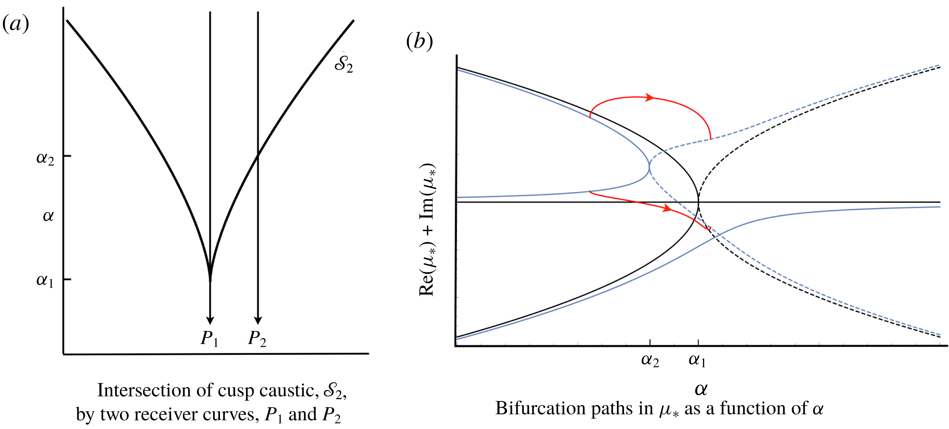
To make these ideas concrete, we have shown a family of three bifurcating rays (in
 $\unicode[STIX]{x1D707}_{\star }$
, for example) along two receiver curves
 $\boldsymbol{x}_{R}(\unicode[STIX]{x1D6FC})$
in figure 2. These rays bifurcate as a result of intersections with a three ray generating cusp caustic shown in figure 2(a). In both cases, the ray family requires two complex branches in order to satisfy the conservation of rays. It is sufficient to use the perturbation to determine the complex rays, however, this figure also demonstrates how the complex continuation generates the same complex rays as the receiver winds around the caustic point
 $\unicode[STIX]{x1D6FC}_{2}$
, when
 $\boldsymbol{x}_{R}$
follows
 $P_{2}$
in figure 2(a).
A key property of the caustics encountered in this paper is that they are locally modelled in terms of a structurally stable member of the catastrophe hierarchy given by Thom (Reference Thom1989). This allows us to model the coalescing parameter branches locally as roots of a polynomial, one of a limited number of so-called normal forms. The roots of the polynomial are equivalent to, and thus represent, the rays. If the rays are tangent at a caustic, the roots coalesce, just as the equivalent parameters
 $\unicode[STIX]{x1D73B}_{\star }$
do.
In this paper we consider only the cuspoids of catastrophe theory (see Poston & Stewart Reference Poston and Stewart2014), so that the normal forms are univariate polynomials that depend continuously on a set of
 $K$
control parameters,
 $\unicode[STIX]{x1D743}$
(functions of
 $\boldsymbol{x}_{R}$
), where
 $K+1$
is the polynomial order. The normal form is defined by
 $$\begin{eqnarray}{\mathcal{U}}_{K}(\unicode[STIX]{x1D708};\unicode[STIX]{x1D743})\equiv \unicode[STIX]{x1D708}^{K+1}+\unicode[STIX]{x1D709}_{K}\unicode[STIX]{x1D708}^{K-1}+\unicode[STIX]{x1D709}_{K-1}\unicode[STIX]{x1D708}^{K-2}+\cdots +\unicode[STIX]{x1D709}_{2}\unicode[STIX]{x1D708}+\unicode[STIX]{x1D709}_{1}.\end{eqnarray}$$
Here we assign the order of the polynomial to reflect the structure of the coalescence, which means
 $K+1$
denotes the number of rays tangent (including unphysical conjugate rays) at the caustic, the latter which we now label
 ${\mathcal{S}}_{K}$
. Returning to figure 2, it can be seen that we have cases of a two and three ray coalescence, so that the two appropriate polynomials are
 ${\mathcal{U}}_{1}$
and
 ${\mathcal{U}}_{2}$
, respectively. However, as the ray families in both cases are generating the same continuous caustic in receiver space (see figure 2
a), we may choose to model both families in terms of
 ${\mathcal{U}}_{2}$
. Though the polynomial
 ${\mathcal{U}}_{K}$
is not required explicitly for continuation of the ray family across caustics, the choice of how we model the ray family across the caustic and the precise relation between
 $\unicode[STIX]{x1D743}$
and
 $\boldsymbol{x}_{R}$
play an important part in correcting the ray divergence at caustics.
Two three ray families tracked along receiver curves that intersect a cusp caustic,
 ${\mathcal{S}}_{2}$
. (a) Receiver paths
 $P_{1}$
and
 $P_{2}$
intersect
 ${\mathcal{S}}_{2}$
at
 $\unicode[STIX]{x1D6FC}_{1}$
and
 $\unicode[STIX]{x1D6FC}_{2}$
, respectively. (b) Family of rays tracked along
 $P_{1}$
, black; along
 $P_{2}$
, grey (blue, online). Solid line, real parameters/rays; dashed, complex. Arrowed line (red, online) complex continuation of solutions as
 $\unicode[STIX]{x1D6FC}$
loops around
 $\unicode[STIX]{x1D6FC}_{2}$
.

6.2 Uniform theory
It is well known that ray fields diverge in the vicinity of a caustic. Catastrophe theory replaces the singular rays by a uniform asymptotic expansion valid as
 $k_{0}\rightarrow +\infty$
. The expansion is built in terms of a canonical integral (see Olver et al.
Reference Olver, Olde Daalhuis, Lozier, Schneider, Boisvert, Clark, Miller and Saunders2016, chap. 36),
 $$\begin{eqnarray}\unicode[STIX]{x1D6F9}_{K}(\unicode[STIX]{x1D743})\equiv \int _{-\infty }^{+\infty }\text{e}^{\text{i}\unicode[STIX]{x1D6F7}_{K}(\unicode[STIX]{x1D708};\unicode[STIX]{x1D743})}\,\text{d}\unicode[STIX]{x1D708},\end{eqnarray}$$
where the potential
 $\unicode[STIX]{x1D6F7}_{K}$
is one of four univariate polynomial catastrophes given by Thom (Reference Thom1989), and that we may define here in terms of the normal form (6.1),
 $$\begin{eqnarray}\unicode[STIX]{x1D6F7}_{K}(\unicode[STIX]{x1D708};\unicode[STIX]{x1D743})\equiv \int _{0}^{\unicode[STIX]{x1D708}}{\mathcal{U}}_{K}(\unicode[STIX]{x1D708}^{\prime };\unicode[STIX]{x1D743})\,\text{d}\unicode[STIX]{x1D708}^{\prime }.\end{eqnarray}$$
For example, in the case of
 $K=1,2$
, which we use extensively in this paper and are labelled as a fold and cusp respectively, the catastrophes reduce to more familiar functions, namely the Airy and Pearcey functions, Ai and
 $P$
, respectively (see Olver et al.
Reference Olver, Olde Daalhuis, Lozier, Schneider, Boisvert, Clark, Miller and Saunders2016, chap. 36.2). For example
 $$\begin{eqnarray}\displaystyle & \displaystyle \unicode[STIX]{x1D6F9}_{1}(\unicode[STIX]{x1D709}_{1})\equiv \int _{-\infty }^{+\infty }\text{e}^{\text{i}((1/3)\unicode[STIX]{x1D708}^{3}+\unicode[STIX]{x1D709}_{1}\unicode[STIX]{x1D708})}\,\text{d}\unicode[STIX]{x1D708}=2\unicode[STIX]{x03C0}\text{Ai}(\unicode[STIX]{x1D709}_{1}), & \displaystyle\end{eqnarray}$$
 $$\begin{eqnarray}\displaystyle & \displaystyle \unicode[STIX]{x1D6F9}_{2}(\unicode[STIX]{x1D743})\equiv \int _{-\infty }^{+\infty }\text{e}^{\text{i}((1/4)\unicode[STIX]{x1D708}^{4}+(1/2)\unicode[STIX]{x1D709}_{2}\unicode[STIX]{x1D708}^{2}+\unicode[STIX]{x1D709}_{1}\unicode[STIX]{x1D708})}\,\text{d}\unicode[STIX]{x1D708}=2^{1/2}P(2^{1/2}\unicode[STIX]{x1D709}_{1},\unicode[STIX]{x1D709}_{2}), & \displaystyle\end{eqnarray}$$
otherwise the catastrophes may be computed from the integral expression (6.2) directly.
The correct canonical integral is chosen by identifying the number of rays,
 $K+1$
, at the caustic including the unphysical (conjugate) exponentially growing rays, once the ray computation is made along
 $\boldsymbol{x}_{R}(\unicode[STIX]{x1D6FC})$
. However, the family of rays may be tracked along a curve where the non-caustic rays are close to coalescence and therefore experience divergence, or there may be multiple caustic intersections in
 $\boldsymbol{x}_{R}(\unicode[STIX]{x1D6FC})$
. As we now show these cases may be dealt with trivially by adapting the uniform asymptotics to incorporate all rays found and not just those that are singular at different sections of the curve
 $\boldsymbol{x}_{R}(\unicode[STIX]{x1D6FC})$
.
We begin with the main result of the catastrophe mapping detailed in appendix B. This shows that the ray sum (4.4) may be partitioned into regular (background rays) and singular (divergent at caustic) rays, of which in the latter
 $n_{K}\leqslant K+1$
are physical (either exponentially decaying or real). The singular rays are then replaced by a uniform asymptotic series in
 $\unicode[STIX]{x1D6F9}_{K}$
and its derivatives. Importantly, the uniform asymptotics of the ray field are still local solutions of the linearized Euler equations in the high-frequency limit, however the catastrophe theory map allows us to bypass substitution of
 $\unicode[STIX]{x1D6F9}_{K}$
into these equations directly (see (B 1)). Using (B 1) and (B 5) we may write
 $$\begin{eqnarray}\displaystyle g_{5\unicode[STIX]{x1D702}} & {\sim} & \displaystyle \left(\frac{k_{0}^{2\tilde{\unicode[STIX]{x1D6FD}}}}{2\unicode[STIX]{x03C0}\text{i}}\right)^{1/2}\text{e}^{\text{i}k_{0}A_{CE}}\left(c_{0,0}+\text{e}^{-\text{i}\unicode[STIX]{x03C0}/2}\mathop{\sum }_{j=1}^{K}k_{0}^{-1+\tilde{\unicode[STIX]{x1D70E}}_{j}}c_{j,0}\frac{\unicode[STIX]{x2202}}{\unicode[STIX]{x2202}\tilde{\unicode[STIX]{x1D709}}_{j}}\right)\unicode[STIX]{x1D6F9}_{K}(\tilde{\unicode[STIX]{x1D743}})\nonumber\\ \displaystyle & & \displaystyle +\,\mathop{\sum }_{n_{r}=n_{K}+1}^{N}{\mathcal{A}}_{\unicode[STIX]{x1D702}}^{(n_{r})}P_{0}^{(n_{r})}\text{e}^{\text{i}k_{0}S^{(n_{r})}},\end{eqnarray}$$
where, as in appendix B:
 $\tilde{\unicode[STIX]{x1D743}}$
denote wavenumber scaled control variables
 $\unicode[STIX]{x1D743}$
;
 $c_{0,0},c_{j,0}$
, denote uniform amplitude coefficients;
 $A_{CE}$
denotes a phase variable; and
 $\tilde{\unicode[STIX]{x1D6FD}}$
,
 $\tilde{\unicode[STIX]{x1D70E}}_{j}$
, denote scaling constants dependent on
 $K$
. All variables are functions of
 $\boldsymbol{x}_{R}$
and so vary from point to point. We use the method found in § IV of Connor & Curtis (Reference Connor and Curtis1984) to numerically map the ray field to the uniform constants, e.g.
 $\unicode[STIX]{x1D743}$
,
 $A_{CE}$
at each receiver point.
To address the issue of multiple groups within the ray family coalescing at various points along
 $\boldsymbol{x}_{R}$
, we choose to map all rays found into a uniform series, so that the second term of (6.6) is not required. For example, if the ray solver determines
 $N_{1}$
rays – including unphysical conjugate rays – then
 $N_{1}=K+1$
. This is particularly useful when either: the ray solver is unable to track rays along
 $\boldsymbol{x}_{R}$
for numerical reasons, e.g. poor step size; the number of rays changes discontinuously due to unusual structures in the field (see § 7.2). In the case of the latter, this allows for a piecewise description of the field valid in contiguous sections delimited by this structure.
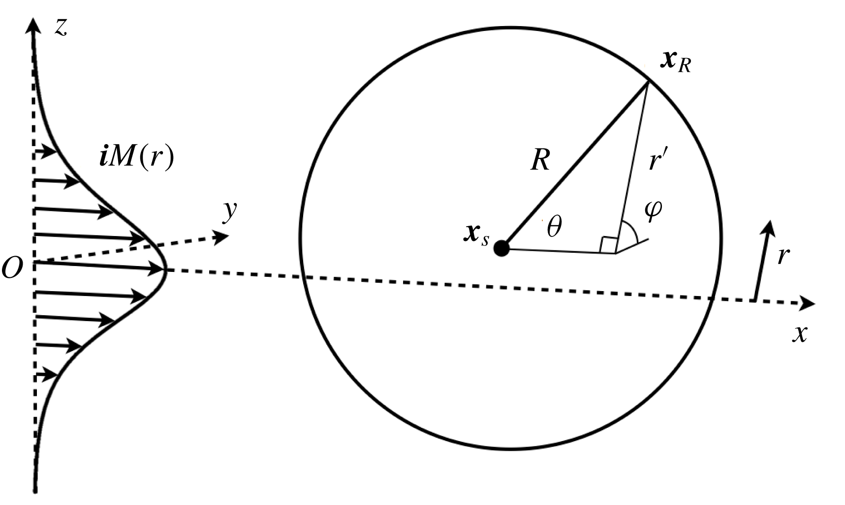
Coordinate geometry with point source
 $\boldsymbol{x}_{s}=(x_{s},y_{s},z_{s})$
and a radially symmetric profile generated by
 $M(r)=M_{J}\text{sech}^{2}(r/r_{J})$
. Coordinates defined in (7.1).

7 Parallel shear flows
In this section we consider computations of the acoustic field generated by a point source embedded in a doubly infinite subsonic isothermal parallel shear flow as shown in figure 3. Although the framework of §§ 2–6 may be applied more generally, as we show in § 8 for a spreading jet, such flows are a useful testbed for our programme, and have been used extensively as mean flow models of slowly spreading unheated jets (see Lilley Reference Lilley1958). To exemplify the efficiency of our ray approach in this section we carry out a parametric study over a range of off-axis source locations and Mach numbers, establishing the persistence and stability of the novel caustic structures first seen in Stone et al. (Reference Stone, Self and Howls2017).
The doubly infinite isothermal parallel shear flows used here are characterized by unidirectional radially symmetric profiles of the form
 $\boldsymbol{M}(\boldsymbol{x})=\boldsymbol{i}\bar{u}_{1}(r)/\bar{c}_{\infty }=\boldsymbol{i}M(r)$
,
 $a(\boldsymbol{x})=a(r)=1$
, for
 $-\infty <x_{1}<+\infty$
, where
 $r$
is a cross-stream radial coordinate and
 $\boldsymbol{i}$
is the unit vector in the direction of flow along the
 $x_{1}$
-axis. For convenience we relabel
 $(x_{1},x_{2},x_{3})=(x,y,z)$
, and define the cylindrical and spherical polar coordinates about a source point
 $\boldsymbol{x}_{s}$
shown in figure 3 as
 $$\begin{eqnarray}\displaystyle \left.\begin{array}{@{}c@{}}\displaystyle \unicode[STIX]{x1D711}=\tan ^{-1}\left(\frac{z-z_{s}}{y-y_{s}}\right),\quad \unicode[STIX]{x1D703}=\cos ^{-1}\left(\frac{x-x_{s}}{R}\right),\\ \displaystyle r=\sqrt{y^{2}+z^{2}},\quad r^{\prime }=\sqrt{(y-y_{s})^{2}+(z-z_{s})^{2}},\quad R=\sqrt{(x-x_{s})^{2}+{r^{\prime }}^{2}},\end{array}\right\} & & \displaystyle\end{eqnarray}$$
where the azimuthal and polar angles are defined in the ranges
 $\unicode[STIX]{x1D711}=[0,2\unicode[STIX]{x03C0})$
,
 $\unicode[STIX]{x1D703}=[0,\unicode[STIX]{x03C0}]$
, respectively.
We construct ray solutions by parameterizing the receiver according to
 $\unicode[STIX]{x1D6FC}=\unicode[STIX]{x1D703}$
with
 $\unicode[STIX]{x1D711},R$
fixed (see § 4), generating cross-sections on the sphere shown in figure 3. Solutions in
 $(\unicode[STIX]{x1D711},\unicode[STIX]{x1D703})$
are then determined by pasting cross-sections together. We use a prototypical parallel shear profile
 $M(r)=M_{J}\text{sech}^{2}(r/r_{J})$
(as used in Wundrow & Khavaran (Reference Wundrow and Khavaran2004) and Stone, Self & Howls (Reference Stone, Self and Howls2014)), where
 $M_{J}$
is the jet centreline Mach number and
 $r_{J}$
the effective jet radius (which is kept constant at
 $r_{J}=1/2$
), so that all necessary flow derivatives required in (3.4)–(3.6), (3.13), (3.14) may be computed analytically. We present our results in terms of the Strouhal number
 $$\begin{eqnarray}St\equiv \frac{k_{0}r_{J}}{\unicode[STIX]{x03C0}a_{J}M_{J}},\end{eqnarray}$$
in addition to the wavenumber
 $k_{0}$
, where
 $a_{J}$
is the jet centreline sound speed ratio and is equal to 1 for isothermal flows.
In the following sections, our primary focus will be on computing
 $g_{5}$
as given by (3.17) and (4.4) with
 ${\mathcal{A}}_{\unicode[STIX]{x1D702}}=1$
as opposed to
 $g_{5\unicode[STIX]{x1D702}}$
. This allows the presentation of our results to be independent of the receiver dependent scalings involved in converting
 $g_{5}$
to each component
 $g_{5\unicode[STIX]{x1D702}}$
(see (A 2)). The result is that the effects of caustics and complex rays are easily visualized, though there is no loss of generality in the application of the ray method.
7.1 Tracking caustics and uniform asymptotics
Our first demonstration of the ray solver’s utility is its ability to locate caustics. In § 6 we suggested caustics as a means of tracking complex rays and as the loci about which we must replace singular rays by an appropriate uniform asymptotic expansion. However, stable caustics also organize the field structurally, so that their location not only indicates regions of high intensity, but also provides the delineations of regions of distinct qualitative behaviour. An important property of the caustic structure calculated for a particular source-flow configuration is that it is generic for all the corresponding vector Green’s function components,
 $g_{\ell \unicode[STIX]{x1D702}}$
, and for all frequencies for which it is evaluated.
In the following we limit the search to caustics generated by real rays, propagating a pseudo-random distribution of angles
 $(\unicode[STIX]{x1D707},\unicode[STIX]{x1D706})$
using the initial value problem (3.4)–(3.6), until they intersect a sphere of radius
 $R$
centred on the source
 $\boldsymbol{x}_{s}$
. We record caustics as points where the ray solutions have Jacobian
 $J$
, of (3.10) approximately zero. As the Jacobian scales with
 $R^{2}$
, a suitable caustic tolerance is
 $J/R^{2}\leqslant \unicode[STIX]{x1D716}_{J}$
,
 $\unicode[STIX]{x1D716}_{J}\ll 1$
.
In this section we will focus on the far field, setting
 $R/r_{J}=O(10^{2})$
to generate a sphere large enough for the caustic surfaces to have converged to their far-field locations in
 $(\unicode[STIX]{x1D711},\unicode[STIX]{x1D703})$
. We limit the polar angular range to
 $\unicode[STIX]{x1D703}\in [0,\unicode[STIX]{x03C0})$
, as an observer at
 $\unicode[STIX]{x1D703}=\unicode[STIX]{x03C0}$
lies approximately on the jet axis in the upstream region where rays remain trapped in the jet. We delay a study of this field until § 7.5, where we show that the trapped rays generate an extremely dense and complicated caustic structure that merits its own analysis.
Figure 4(a) shows the ray endpoints
 $\boldsymbol{x}(\unicode[STIX]{x1D73B})$
of the propagated pseudo-random distribution overlaid with detected caustics for a source at
 $r_{s}=0.75$
with Mach number
 $M_{J}=0.9$
. Here a high density of rays indicates a caustic as the ray paths are closely grouped together compressing the infinitesimal ray area described by the Jacobian,
 $J$
. However, this correspondence is not sufficient to calculate the caustic alone and must be supplemented with the
 $J=0$
condition described above.
From figure 4(a) we immediately identify two well-separated caustic structures inhabiting two distinct regions of the receiver coordinates and whose positions are symmetric about the line
 $\unicode[STIX]{x1D711}=\unicode[STIX]{x03C0}$
. The first, a broadly smooth fold caustic,
 ${\mathcal{S}}_{1}$
, generated by two rays, with cusp-like kinks lies in the downstream region,
 $\unicode[STIX]{x1D703}\leqslant \unicode[STIX]{x03C0}/2$
. The second, is a large cusp caustic that dominates upstream angles,
 $\unicode[STIX]{x1D703}>\unicode[STIX]{x03C0}/2$
. Starting with the latter, we perform a local analysis using the boundary value problem (4.1). Three generating rays are detected confirming that this is indeed a cusp caustic,
 ${\mathcal{S}}_{2}$
, with uniform asymptotics based upon the Pearcey function (6.5).
Far-field ray densities and amplitude
 $|g_{5}|$
as a function of
 $(\unicode[STIX]{x1D711},\unicode[STIX]{x1D703})$
. Solid line, loci of caustics. Dashed line,
 $\unicode[STIX]{x1D703}_{S}$
. (a) Real ray path intersections with far-field sphere. Inset describes local structure of real caustic evaporation
 $(\unicode[STIX]{x1D711}_{S},\unicode[STIX]{x1D703}_{S})$
, evaporation point;
 $(\unicode[STIX]{x1D711}_{S}^{\prime },\unicode[STIX]{x1D703}_{S})$
, non-tangential intersection. (b) Total ray field,
 $|g_{5}|$
, with parameters
 $r_{s}=0.75$
,
 $M_{J}=0.9$
,
 $k_{0}=30$
,
 $St=5.3$
. (c) Scale of amplitude shown in (b).

The downstream caustic is more complicated than that in the upstream. First, it does not provide a continuous delimitation of the cone of silence, a shadow zone which is indicated by figure 4(a) as the downstream region absent of real rays. Instead, the caustic appears to terminate, or evaporate, at two angular points, which we denote by
 $(\unicode[STIX]{x1D711}_{S},\unicode[STIX]{x1D703}_{S})$
and
 $(2\unicode[STIX]{x03C0}-\unicode[STIX]{x1D711}_{S},\unicode[STIX]{x1D703}_{S})$
, with the latter due to symmetry. The cone of silence boundary is thus a mixture of caustic and the line
 $\unicode[STIX]{x1D703}_{S}$
, the latter whose significance we discuss below. Second, a magnified view of the caustic evaporation, inset of figure 4(a), shows that near to the caustic evaporation, the cusp-like kinks are in fact cusp caustics,
 ${\mathcal{S}}_{2}$
, generated by three real rays which are present in the region delimited by the cusp and
 $\unicode[STIX]{x1D703}_{S}$
.
Real ray numbers about the downstream caustic evaporation (cf. figure 4
a). Real ray numbers are discontinuous across
 $\unicode[STIX]{x1D703}_{S}$
, which is not a caustic. Arrows indicate how piecewise uniform asymptotics is applied:
 $\unicode[STIX]{x1D703}<\unicode[STIX]{x1D703}_{S}$
, class as
 ${\mathcal{S}}_{1}$
and use
 $\unicode[STIX]{x1D6F9}_{1}$
;
 $\unicode[STIX]{x1D703}>\unicode[STIX]{x1D703}_{S}$
, class as
 ${\mathcal{S}}_{2}$
and use
 $\unicode[STIX]{x1D6F9}_{2}$
.

The line
 $\unicode[STIX]{x1D703}_{S}$
introduces an unusual structural element to the field, which we deal with by using piecewise uniform asymptotics. This is summarized in figure 5 according to the number of real rays found about the downstream cusp. There is clearly a discontinuity in the number of real rays crossing
 $\unicode[STIX]{x1D703}_{S}$
that is not accountable to numerics but rather a physical effect of ray refraction (see § 7.3). Although we show in § 7.4 that the true local behaviour is governed by a catastrophe-like integral first described in Stone et al. (Reference Stone, Self and Howls2017) and that closer inspection reveals a complex ray generated caustic nearby, the uniform asymptotics of (6.6) does not incorporate this integral and we must proceed with a piecewise description according to figure 5.
Using the caustic structures of figure 4(a), we make a total ray calculation whose amplitude is shown in figure 4(b). Cross-sections of figure 4(b) have previously been benchmarked against modal solutions of Lilley’s equation in Stone et al. (Reference Stone, Self and Howls2014). A comparison of figure 4(a,b) shows that, outside of the cone of silence and away from the caustics, the amplitude of the field is not a simple function of the density of rays. Rather the field amplitude is the resultant of the superposition of the ray-transported phases. Additionally, figure 4(b) shows that the field is non-zero in the cone silence, albeit exponentially decaying, with the former a value that may not be inferred from figure 4(a), thus establishing the need for complex rays.
Cross-sections of
 $|g_{5}|\times 10^{3}$
as a function of
 $\unicode[STIX]{x1D703}$
for
 $r_{s}=0.75$
,
 $M_{J}=0.9$
,
 $k_{0}=30$
,
 $St=5.3$
for (a)
 $\unicode[STIX]{x1D711}=0$
, (b)
 $\unicode[STIX]{x1D711}=\unicode[STIX]{x03C0}/3$
, (c)
 $\unicode[STIX]{x1D711}=\unicode[STIX]{x03C0}/2\approx \unicode[STIX]{x1D711}_{S}$
, (d)
 $\unicode[STIX]{x1D711}=7\unicode[STIX]{x03C0}/10$
, (e)
 $\unicode[STIX]{x1D711}=5\unicode[STIX]{x03C0}/6$
, (f)
 $\unicode[STIX]{x1D711}=\unicode[STIX]{x03C0}$
. Key: grey (blue, online) ray; black, uniform (which overlies the modal solution of Lilley’s equation as shown in Stone et al. (Reference Stone, Self and Howls2014)). Intersections with structures in figure 4(b):
 $\unicode[STIX]{x1D703}_{f}$
, downstream caustic;
 $\unicode[STIX]{x1D703}_{c}$
, upstream cusp;
 $\unicode[STIX]{x1D703}_{S}$
, as in figure 4(b).

7.2 Amplitude cross-sections
We now demonstrate the use of uniform asymptotics as described in § 6 by correcting the singularities generated by the caustics in figure 4. In particular, we begin to elicit the significance of the line
 $\unicode[STIX]{x1D703}_{S}$
and how it structurally delimits the field in the manner of caustic, but with no attendant singularity.
We start by taking cross-sections of the Green’s function shown in figure 4, for constant
 $\unicode[STIX]{x1D711}$
in the range
 $0\leqslant \unicode[STIX]{x1D711}\leqslant \unicode[STIX]{x03C0}$
(due to symmetry), as a function of
 $\unicode[STIX]{x1D703}\in [0,\unicode[STIX]{x03C0})$
. It is expedient for our discussion to split figure 6, showing these cross-sections, into three groups.
The first group, figure 6(a,b), intersects both the upstream and downstream caustics at
 $\unicode[STIX]{x1D703}_{c}$
and
 $\unicode[STIX]{x1D703}_{f}$
, respectively. For the latter we use a subscript
 $f$
to denote any intersection with largely fold caustic downstream even with the cusp part when necessary. In the vicinity of these caustics, the ray solution diverges significantly; a feature which is then corrected upon using the appropriate uniform asymptotics: Airy, (6.4), for the fold intersection downstream and Pearcey, (6.5), for the cusp upstream. At sufficient distance from the caustic both the ray and uniform solutions agree as they are asymptotically equal in non-singular regions.
It is clear from the figures discussed so far, that the line
 $\unicode[STIX]{x1D703}_{S}$
plays a key role in washing out the downstream oscillations abruptly, as is also evident from the global solution plotted in figure 4(b). In the previous section, we noted that real ray numbers are discontinuous upon crossing
 $\unicode[STIX]{x1D703}_{S}$
. Once complex rays are included, we may qualify this as the real rays transition into complex ones, hence the oscillations washing out rather than a discontinuity in the field.
Aside from crossing
 $\unicode[STIX]{x1D703}_{S}$
the inclusion of complex rays in figures 6(a) and 6(b) derives from a local tracking across the caustics. For instance, the cone of silence field
 $\unicode[STIX]{x1D703}<\unicode[STIX]{x1D703}_{f}$
is generated by an exponentially small ray, so that the ray field decays with increasing distance from
 $\unicode[STIX]{x1D703}_{f}$
. In the upstream region, another exponentially small complex ray is generated as the receiver crosses the cusp in the direction of decreasing
 $\unicode[STIX]{x1D703}$
.


The second group in our discussion contains only figure 6(c). At this point the downstream caustic intersection is near evaporation, i.e.
 $(\unicode[STIX]{x1D711}=\unicode[STIX]{x03C0}/2,\unicode[STIX]{x1D703}_{f})\approx (\unicode[STIX]{x1D711}_{S},\unicode[STIX]{x1D703}_{S})$
. For this source and Mach number, the evaporation point lies very close to the downstream cusps as can be seen from figure 4(b). In this case both the ray and uniform solutions are similar, as the latter which uses an Airy function to correct the ray field fails to model the evaporation adequately. This is a consequence of using piecewise uniform asymptotics to correct an evaporation that is really modelled by a generalization of the cuspoids as discussed in § 6. These evaporations are highly localized in
 $(\unicode[STIX]{x1D711},\unicode[STIX]{x1D703})$
and so errors such as that shown in 6(c) do not undermine the ray calculations.
The significance of the coalescence of intersections
 $\unicode[STIX]{x1D703}_{f}$
and
 $\unicode[STIX]{x1D703}_{S}$
, and subsequent disappearance of
 $\unicode[STIX]{x1D703}_{f}$
from cross-sections, is shown in the third group: figure 6(d–f). The downstream oscillations are no longer present and continuation into the cone of silence is via
 $\unicode[STIX]{x1D703}_{S}$
. As before, crossing
 $\unicode[STIX]{x1D703}_{S}$
generates an exponentially small complex ray at the expense of a real ray. This complex ray is much smaller in magnitude than the corresponding complex ray generated in the cone of silence when passing across
 $\unicode[STIX]{x1D703}_{f}$
. This is due to the absence of a caustic effecting an intensity rise and leads to two distinct magnitudes of complex ray solutions in the cone of silence.
Unlike the downstream caustic, the upstream cusp caustic is still present in figure 6(d–f). In the discussion of upstream caustics, figure 6(f) is the most significant as it depicts the intersection through the upstream cusp’s symmetry line
 $\unicode[STIX]{x1D711}=\unicode[STIX]{x03C0}$
, where all three generating rays are tangent and singular. Here the uniform upstream field is at a maximum and commensurate with the amplitudes of the downstream caustics. This peak field can be seen in finer detail in figure 7 for a small angular range about the cusp point. The corrections made by uniform asymptotics show how the true peak field sits behind the caustic, while providing a subtle realignment of oscillations on the lower side of the cusp that one cannot visualize from cross-sections alone.
Uniform computations of Green’s function components as a function of Strouhal number (
 $0.5\leqslant St\leqslant 10$
) for an off-axis source and receiver coordinates
 $\unicode[STIX]{x1D711}=0,\unicode[STIX]{x1D703}=[0,\unicode[STIX]{x1D703}_{S}]$
. The field
 $\unicode[STIX]{x1D703}<\unicode[STIX]{x1D703}_{f}$
is generated by complex rays;
 $\unicode[STIX]{x1D703}>\unicode[STIX]{x1D703}_{f}$
generated by reals rays. Scale as in figure 4(c).

In the final part of this section we address the suitability of incorporating complex rays in ray-based solvers used for flow–acoustic interaction effects. Starting with figure 6, it is clear that complex ray contributions are small in magnitude and that on these grounds we might be tempted to neglect them. However, these contributions are evaluated using large wavenumbers particularly to elicit the characteristic exponential decay of physical complex rays and oscillations generated by multiple real rays. The study shown in figure 8 shows how these features vary as a function of Strouhal number for three Green’s function components generated by an off-axis source evaluated on the curve
 $\unicode[STIX]{x1D711}=0,\unicode[STIX]{x1D703}=[0,\unicode[STIX]{x1D703}_{S}]$
. In each case, at the lower end of the Strouhal range,
 $St=0.5$
(a suitable lower bound according Wundrow & Khavaran (Reference Wundrow and Khavaran2004), see § 1), the complex field
 $\unicode[STIX]{x1D703}<\unicode[STIX]{x1D703}_{f}$
in the cone of silence is largely commensurate in magnitude with the real ray field
 $\unicode[STIX]{x1D703}>\unicode[STIX]{x1D703}_{f}$
. Only at large Strouhal numbers does exponential decay become readily apparent, thus indicating that complex rays are important for accurate downstream computations across broad frequency ranges.
Real part of (contributing) ray paths generating the downstream fold caustic,
 ${\mathcal{S}}_{1}$
, on
 $\boldsymbol{x}_{R}(\unicode[STIX]{x1D703})$
;
 $\unicode[STIX]{x1D711}$
,
 $R$
, fixed. (a)
 $\unicode[STIX]{x1D703}<\unicode[STIX]{x1D703}_{f}$
, one complex ray (red).
 $\unicode[STIX]{x1D703}_{f}<\unicode[STIX]{x1D703}<\unicode[STIX]{x1D703}_{S}$
, two real rays (blue).
 $\unicode[STIX]{x1D703}_{S}<\unicode[STIX]{x1D703}$
, one real (blue) and one complex (grey). (b) Close up of ray paths projected into
 $xz$
-plane describes the continuation and coalescence of
 $\unicode[STIX]{x1D703}_{S}$
and caustic in the near field. (c) Solid arrowed line denotes structural intersections made by
 $\boldsymbol{x}_{R}$
in (a) with caustics (black line), where
 $(\unicode[STIX]{x1D711}_{S},\unicode[STIX]{x1D703}_{S})$
denotes evaporation.

Real part of (contributing) ray paths generating a downstream cusp on the receiver curve
 $\boldsymbol{x}_{R}(\unicode[STIX]{x1D703})$
;
 $\unicode[STIX]{x1D711}$
,
 $R$
, fixed. (a)
 $\unicode[STIX]{x1D703}_{S}\leqslant \unicode[STIX]{x1D703}<\unicode[STIX]{x1D703}_{f}$
, three real rays (blue).
 $\unicode[STIX]{x1D703}_{f}<\unicode[STIX]{x1D703}\leqslant \unicode[STIX]{x1D703}_{c}$
, one real (blue) and one complex (red). Rays in bold denote cusp real ray triplet at particular receiver point. (b) Solid arrow line denotes structural intersections made by
 $\boldsymbol{x}_{R}$
in (a) with caustic (black line). Dashed arrowed line, alternative path which discovers complex ray generated caustic (purple solid line).

7.3 Caustic generating rays
While § 7.1 provides a structural explanation of the point source field behaviour in terms of caustics, the ray paths offer a geometric perspective. This is perhaps the outstanding virtue of the ray method as it allows us to summarize new structural features such as the line
 $\unicode[STIX]{x1D703}_{S}$
, in a visual manner. Here we shall focus on the rays generating the downstream caustic as this contains the most interesting novel behaviour from the ray perspective.
Figures 9 and 10 plot the real part of the ray paths for the two receiver positions as a function of
 $\unicode[STIX]{x1D703}$
at constant
 $\unicode[STIX]{x1D711}$
,
 $R$
. These solutions, collected on a receiver radius
 $R=7$
, are nominally in the near field (see § 7.5) the better to illustrate the refractive effects of the flow upon the ray paths. However, there is no loss of generality as the mechanisms behind the generating rays shown are the same as those in the far field for the range of angles shown.
Figure 9 describes the intersection of the receiver curve with the downstream caustic, so that a generic intersection
 $\unicode[STIX]{x1D703}_{f}$
is modelled locally by a fold catastrophe
 $\unicode[STIX]{x1D6F9}_{1}$
according the piecewise description of the caustic shown in figure 5.
Traversing the receiver curve of figure 9, starting from small polar angles
 $\unicode[STIX]{x1D703}<\unicode[STIX]{x1D703}_{f}$
that lie in the cone of silence, we collect one exponentially small complex ray contribution (red). This solution then coalesces with its unphysical conjugate (not shown) to generate a real ray pair (blue) at the caustic
 $\unicode[STIX]{x1D703}_{f}$
, so that oscillations may exist between
 $\unicode[STIX]{x1D703}_{f}<\unicode[STIX]{x1D703}<\unicode[STIX]{x1D703}_{S}$
in the ray amplitude as the solutions are superposed. As
 $\unicode[STIX]{x1D703}_{S}$
is crossed, one of these real ray pairs transitions into an exponentially decaying complex ray (grey), thereby causing the washing out of oscillations. The ray field for
 $\unicode[STIX]{x1D703}>\unicode[STIX]{x1D703}_{S}$
is then composed of one real ray (blue) and one complex ray (grey). We may interpret this transition physically in terms of the flow’s ability to refract rays towards the receiver. For example, the flow cannot refract a second real ray upwards indefinitely and so this second ray disappears; except it really transitions into a complex ray rather than disappearing.
We now investigate the ray paths generating the downstream caustic about its cusps. These paths shown in figure 10 describe intersections of the downstream caustic, again denoted by
 $\unicode[STIX]{x1D703}_{f}$
, where we model it using
 $\unicode[STIX]{x1D6F9}_{2}$
(see figure 5). Here the triplet of rays in the centre of the cusp transition into a real ray and a conjugate pair across the caustic, where the physical contributing complex ray is plotted for clarity.
The complex rays (red) shown in figure 10(a) may be continued from
 $\unicode[STIX]{x1D703}_{f}$
along an alternative path shown in figure 10(b) by the dashed arrowed line, in order to investigate the puzzling evaporation of the caustic at
 $(\unicode[STIX]{x1D711}_{S},\unicode[STIX]{x1D703}_{S})$
. The solutions then show that there is another caustic sprouting out symmetrically from
 $(\unicode[STIX]{x1D711}_{S},\unicode[STIX]{x1D703}_{S})$
, but generated by complex rays. This complex caustic would also appear if the same excursions were made by the receiver in figure 9. We discuss the full details of the downstream cusps in § 7.4, below.
7.4 Parametric analysis and generalized cuspoid catastrophe
In this section we carry out a parametric analysis in order to explore the dependence of the far-field caustics on source radius,
 $r_{s}$
, and Mach number,
 $M_{J}$
, with special reference to the downstream cusp. As discussed above, caustics describe the loci of high intensity due to propagation through the mean flow, and so understanding caustic behaviour as these physical parameters are varied is of great benefit.
Figure 11(a) shows the caustic positions in
 $(\unicode[STIX]{x1D711},\unicode[STIX]{x1D703})$
for four source positions with fixed Mach number,
 $M_{J}=0.9$
, while figure 11(b) studies the caustic behaviour as
 $M_{J}$
is varied for two source radii. These figures show that the caustics described in figure 4(b) are present and symmetric about
 $\unicode[STIX]{x1D711}=\unicode[STIX]{x03C0}$
for all parameters shown. This includes Mach numbers as low as
 $M_{J}=0.05$
, demonstrating the persistence expected from the stable caustics of catastrophe theory.
Of the caustics shown in these parametric studies, we will focus on the downstream behaviour first, as the peculiarities of the solution shown in figure 4 are again present. The key to this structure is that, although it persists for all source positions and Mach numbers shown in figure 11, the precise details of the caustic do change. For instance, figure 11(a) shows that for the same Mach number
 $M_{J}=0.9$
, the source position
 $r_{s}=0.5$
lying on the lip line has no downstream cusps, yet they exist for
 $r_{s}=0.75,1.5,2.5$
.
The reason for the presence or absence of cusps is that the downstream caustic about its evaporation points is governed by a more complicated local ray behaviour leading to a generalization of the cuspoid hierarchy described in § 6.2. This local form, derived in Stone et al. (Reference Stone, Self and Howls2017), is given by
 $$\begin{eqnarray}{\mathcal{I}}(\bar{\unicode[STIX]{x1D743}})\sim k_{0}^{1/2}\int _{0}^{+\infty }\text{e}^{-\text{i}k_{0}(\unicode[STIX]{x1D708}^{4}+\bar{\unicode[STIX]{x1D709}}_{2}\unicode[STIX]{x1D708}^{2}+\bar{\unicode[STIX]{x1D709}}_{1}\unicode[STIX]{x1D708}+\bar{\unicode[STIX]{x1D709}}_{0}\ln \unicode[STIX]{x1D708})}\,\text{d}\unicode[STIX]{x1D708},\quad \bar{\unicode[STIX]{x1D743}}=(\bar{\unicode[STIX]{x1D709}}_{0},\bar{\unicode[STIX]{x1D709}}_{1},\bar{\unicode[STIX]{x1D709}}_{2}).\end{eqnarray}$$
Parametric study of real ray generated far-field caustics. Solid line, caustics; horizontal dashed line,
 $\unicode[STIX]{x1D703}_{S}$
;
 $\unicode[STIX]{x1D703}^{\ast }$
, cone of silence angle. Arrows indicate increasing parameter. (a) A function of source radius (
 $r_{s}=0.5,0.75,1.5,2.5$
) for constant Mach number
 $M_{J}=0.9$
. Thick solid line,
 $r_{s}=2.5$
. Shaded region, cone of silence for
 $r_{s}=2.5$
. (b) A function of Mach number (
 $M_{J}=0.05,0.1,0.3,0.7$
). For
 $r_{s}=0.75$
,
 $0\leqslant \unicode[STIX]{x1D711}\leqslant \unicode[STIX]{x03C0}$
;
 $r_{s}=2.5$
,
 $\unicode[STIX]{x03C0}\leqslant \unicode[STIX]{x1D711}\leqslant 2\unicode[STIX]{x03C0}$
.

The original idea for the local form (7.3) arose from a careful study of the (real and complex) ray dynamics generated by the solver as detailed in § 7.3 in the vicinity of the evaporation point
 $(\unicode[STIX]{x1D711}_{S},\unicode[STIX]{x1D703}_{S})$
. For example, in figure 10 local analysis using (4.1) shows the existence of a complex cusp caustic sprouting from the evaporation thus indicating the existence of a higher-order (
 $K>2$
) caustic than the cusp so far considered.
Despite the appearance of the logarithm in the exponent, the caustic structure contained within (7.3) is structurally stable and may be mapped to a swallowtail caustic,
 ${\mathcal{S}}_{3}$
, generated by four rays (see Olver et al. (Reference Olver, Olde Daalhuis, Lozier, Schneider, Boisvert, Clark, Miller and Saunders2016), chap. 36.4 and § 6.2 with
 $K=3$
). The downstream caustics present in the vector Green’s function then result from intersections of the receiver surface with the swallowtail caustic. The magnitude of the source radius
 $r_{s}$
controls whether the intersection is smooth or cusped. However, whichever intersection is taken,
 ${\mathcal{I}}$
incorporates the effects of
 $\unicode[STIX]{x1D703}_{S}$
, which we have so far treated using (6.6) in a piecewise manner.
In order to illustrate the existence of smooth or cusped downstream caustics, figure 12 plots the function
 ${\mathcal{I}}$
of (7.3) for three source radii,
 $r_{s}=0.5,0.75,1.5$
, with fixed Mach number,
 $M_{J}=0.9$
, whose global caustic structures are shown in figure 11(a) (cf. figure 4). Here we have used the mappings defined in Stone et al. (Reference Stone, Self and Howls2017) to express the coefficients
 $\bar{\unicode[STIX]{x1D743}}$
as functions of
 $(\unicode[STIX]{x1D711},\unicode[STIX]{x1D703})$
. The mapping describes the caustic structure in the region
 $\unicode[STIX]{x1D711}=[0,\unicode[STIX]{x03C0}]$
, with no loss of generality for describing the behaviour about the evaporation point in the region
 $\unicode[STIX]{x1D711}=[\unicode[STIX]{x03C0},2\unicode[STIX]{x03C0}]$
.
These figures confirm the local geometric ray analysis of section § 7.3. For all cases of source radii shown, even those that do not lead to downstream cusps, e.g.
 $r_{s}=0.5$
, the caustics do not really disappear, but transition from coalescences between real rays into coalescences between exponentially decaying complex rays when the caustic is tangential with
 $\unicode[STIX]{x1D703}_{S}$
. Consequently the corresponding branch of the caustic does not generate a significant intensity rise in the field, so that the field appears asymmetric in amplitude about the evaporation (
 $\unicode[STIX]{x1D711}_{S},\unicode[STIX]{x1D703}_{S}$
). The resolution of caustics beyond evaporation is simply a matter of exponentially small complex rays that are not accounted for in our real ray caustic-finding algorithm, but may be found using the full machinery of §§ 4 and 5. This becomes apparent if we compare the caustics of figures 5 and 12(c).
As shown in figure 12, not only does
 $r_{s}$
control the existence of downstream cusps (they exist for
 $r_{s}\gtrsim 0.7$
), but also the magnitude of their protrusion above
 $\unicode[STIX]{x1D703}_{S}$
. This makes an interesting comparison with the equivalent upstream structure. In the upstream the cusp is a function of both
 $r_{s}$
and
 $M_{J}$
, moving toward the downstream region as either of these parameters is increased, with the cusp point reaching a limiting value of
 $\unicode[STIX]{x1D703}=\unicode[STIX]{x03C0}/2$
as
 $r_{s}\rightarrow +\infty$
and
 $M_{J}\rightarrow 1$
. However, the downstream cusp’s behaviour is controlled predominantly by
 $r_{s}$
and is less dependent on the Mach number
 $M_{J}$
. This is confirmed by figure 11(b), which shows that the protrusion of the downstream cusps (when they exist) is effectively constant for each of the caustics sets with
 $r_{s}$
varied and Mach number constant.
Magnitude of local form
 $|{\mathcal{I}}|$
, (7.3), in (
 $\unicode[STIX]{x1D711},\unicode[STIX]{x1D703}$
) about the caustic evaporation,
 $(\unicode[STIX]{x1D711}_{S},\unicode[STIX]{x1D703}_{S})$
, with
 $M_{J}=0.9$
,
 $k_{0}=30$
,
 $St=5.3$
. Solid line, caustic; dashed line,
 $\unicode[STIX]{x1D703}_{S}$
. (a) Fold intersection. (b) Cusps begin to appear. (c) Cusped intersection. Scale as in figure 4(c).

So far we have not described the parametric behaviour of
 $\unicode[STIX]{x1D703}_{S}$
in figures 11 and 12. We know that this
 $\unicode[STIX]{x1D711}$
-invariant line plays an important structural role in the behaviour of the ray solution as the tangential intersection of
 $\unicode[STIX]{x1D703}_{S}$
with the real ray generated section of the downstream caustic causes its evaporation (cf. figure 12). In the following we show that the behaviour of
 $\unicode[STIX]{x1D703}_{S}$
as a function of flow parameters is extremely simple and that in addition to the source radius
 $r_{s}$
and the angle
 $\unicode[STIX]{x1D703}^{\ast }$
, which we define below, controls the main features of the downstream caustic.
The theoretical position of the line
 $\unicode[STIX]{x1D703}_{S}$
in an isothermal parallel flow may be deduced from the local form (7.3) and the mappings from
 $\bar{\unicode[STIX]{x1D743}}$
to
 $(\unicode[STIX]{x1D711},\unicode[STIX]{x1D703}_{S})$
shown in Stone et al. (Reference Stone, Self and Howls2017). As shown therein
 $$\begin{eqnarray}\bar{\unicode[STIX]{x1D709}}_{0}(\unicode[STIX]{x1D703};M_{J})\propto 1-2M_{J}\cos \unicode[STIX]{x1D703}+(M_{J}^{2}-1)\cos ^{2}\unicode[STIX]{x1D703},\end{eqnarray}$$
where
 $\unicode[STIX]{x1D703}_{S}$
corresponds to
 $\bar{\unicode[STIX]{x1D709}}_{0}=0$
. The physical root is then given by
 $$\begin{eqnarray}\unicode[STIX]{x1D703}_{S}=\cos ^{-1}\left(\frac{1}{1+M_{J}}\right).\end{eqnarray}$$
This makes for an interesting comparison with the well-known cone of silence angle given in the literature (see Goldstein Reference Goldstein1976, p. 270),
 $$\begin{eqnarray}\unicode[STIX]{x1D703}^{\ast }=\cos ^{-1}\left(\frac{1}{1+M_{s}}\right),\end{eqnarray}$$
where
 $M_{s}$
is the Mach number at the source. In the far-field ray solution,
 $\unicode[STIX]{x1D703}^{\ast }$
gives the minimum polar angle obtainable by the downstream caustic. The majority of downstream caustic then effectively sits in the polar range
 $\unicode[STIX]{x1D703}^{\ast }<\unicode[STIX]{x1D703}<\unicode[STIX]{x1D703}_{S}$
as shown by figure 11.
The key difference between these angles is that
 $\unicode[STIX]{x1D703}_{S}$
is independent of source position and varies only as a function of
 $M_{J}$
, whereas
 $\unicode[STIX]{x1D703}^{\ast }$
is a function of both (since
 $M_{s}=M_{J}\text{sech}^{2}(r_{s}/r_{J})$
). This is verified by figure 11(a) as
 $\unicode[STIX]{x1D703}_{S}$
is invariant for the source positions shown and figure 11(b) where
 $\unicode[STIX]{x1D703}_{S}$
is the same when the two different sources have the same Mach number.
Near-field ray solution
 $|R\text{e}^{-\text{i}k_{0}R}g_{5}|$
in an annulus sector
 $1\leqslant R\leqslant 15$
,
 $0\leqslant \unicode[STIX]{x1D703}\leqslant 5\unicode[STIX]{x03C0}/12$
,
 $\unicode[STIX]{x1D711}=0$
, for two source radii. Here
 $O$
denotes the origin at the source
 $\boldsymbol{x}_{s}$
. White line, fold caustic,
 ${\mathcal{S}}_{1}$
; white dashed line,
 $\unicode[STIX]{x1D703}_{S}$
. (a)
 $r_{s}=0.75$
,
 $k_{0}=30$
,
 $St=5.3$
. (b)
 $r_{s}=0.75$
,
 $k_{0}=50$
,
 $St=8.8$
. (c)
 $r_{s}=1.5$
,
 $k_{0}=30$
,
 $St=5.3$
. Scale as in figure 4(c).

7.5 Caustics in the near field
From the preceding section it is clear that interaction of the downstream caustic and the structure defined by
 $\unicode[STIX]{x1D703}=\unicode[STIX]{x1D703}_{S}$
leads to the characteristic behaviour of restricted oscillations and an apparently evaporating caustic. We may study the behaviour of these downstream structures further by considering their near-field behaviour. This also demonstrates another advantage of the high-frequency solution developed in this paper, as unlike some analytical methods (see Mani, Gliebe & Balsa Reference Mani, Gliebe and Balsa1978; Wundrow & Khavaran Reference Wundrow and Khavaran2004), the rays are not restricted to the far field and are valid to within a wavelength of the point source.
Here we consider the near field in the range
 $1\leqslant R\leqslant 15$
. Where the lower bound
 $R=1$
is larger than a distance equal to a wavelength from the source for the wavenumbers considered, and the upper bound
 $R=15$
is nominally chosen as large enough to demonstrate the convergence of the ray structures to their far-field positions in
 $(\unicode[STIX]{x1D711},\unicode[STIX]{x1D703})$
. In addition, we normalize Green’s function by dividing
 $g_{5}$
by
 $\text{exp}(\text{i}k_{0}R)/R$
, thus eliminating the point source singularity that scales as
 $O(1/R)$
.
Figure 13 shows two such near-field ray solutions for source radii
 $r_{s}=0.75,1.5$
with Mach number
 $M_{J}=0.9$
and
 $\unicode[STIX]{x1D711}=0$
. The first two figures, (a) and (b), demonstrate how the downstream fold caustic,
 ${\mathcal{S}}_{1}$
, and the line
 $\unicode[STIX]{x1D703}_{S}$
continue into the near field and coalesce before reaching the point source. We recognize this coalescence as that indicated by the ray paths in figure 9(b). With further reductions in radius,
 $R$
, the downstream field is free from caustics, and there is no cone of silence.
Figure showing a sample of trapped rays and their corresponding Jacobian values as they propagate in the upstream region. Rays confined to approximate polar region
 $\unicode[STIX]{x1D6FF}\unicode[STIX]{x1D703}$
dependent on
 $R$
such that
 $\unicode[STIX]{x1D6FF}\unicode[STIX]{x1D703}\rightarrow 0$
as
 $R\rightarrow +\infty$
. Inset, scale of Jacobian magnitude,
 $|J|$
, determined using (3.10). Small
 $|J|$
corresponds to high amplitude.

It is evident from figure 13 that the downstream near-field structures maintain a measure of self-similarity to those of the downstream far field up until the caustic disappears close to the source. However, the same cannot be said of the upstream region as the near-field high-frequency solution is complicated by so-called trapped rays that remain within the jet. As we now show, this proliferation of rays makes an application of the ray summation and uniform asymptotics of § 4 difficult.
Our first step is to demonstrate geometrically the trapped ray field. Figure 14 shows a sample of trapped rays propagated from the source
 $\boldsymbol{x}_{s}$
. These rays oscillate both in position and amplitude as they are channelled by the jet in the upstream direction. The periodicity of the amplitude between singular (i.e.
 $J=0$
of (3.10)) and finite values along each ray, coupled with the large number of solutions that increase the likelihood of ray path tangency, leads to the formation of a dense caustic network. This caustic network may be calculated using the caustic identification scheme of § 7.1 with caustic points recorded along the ray and not just at the ray endpoints. For example, figure 15 shows the data points of all numerically determined trapped ray caustics for a particular flow–source configuration projected into the
 $y$
-plane. The ordered caustic network shown by figure 15 is perhaps surprising give the extremely complicated and disordered ray paths that generate it.
Locally hyperbolic umbilic (HU) structures in the
 $y=0$
plane with
 $-12D_{J}\leqslant x\leqslant 0$
and point source at
 $\boldsymbol{x}_{s}=(0,0,0.75)$
. Points denote caustic locations projected into
 $y$
-plane. Solid line, hyperbolic umbilic caustics; numbers denote position of HUs in sequence. Dotted line, constant source radius. Inset shows equivalent undeformed hyperbolic umbilic, delineating three regions,
 $\unicode[STIX]{x1D6FA}^{(1,2,3)}$
, of distinct ray contributions.

A full analysis of this caustic network, particularly using (4.1) – though not impossible – is made difficult by the large number of generating rays and the small step size required in receiver position to resolve the densely packed caustics. However, there are two key features shown in figure 15 that we may explore with little difficulty. The first is that the upstream cusp in the far-field solution (e.g. that shown in figure 4), which is a surface in
 $(R,\unicode[STIX]{x1D703},\unicode[STIX]{x1D711})$
, is an extension of the near-field trapped ray network.
The second feature is that the network contains a sequence of increasingly compressed cusps close to fold caustics. This is the signature of a hyperbolic umbilic catastrophe generated by four rays (see Olver et al.
Reference Olver, Olde Daalhuis, Lozier, Schneider, Boisvert, Clark, Miller and Saunders2016, chap. 36.2), locally delineating three regions
 $\unicode[STIX]{x1D6FA}^{(1,2,3)}$
as also shown for clarity in figure 15 (cf. Grikurov (Reference Grikurov1980)). Even though figure 15 shows a visually separated fold and cusp, modelling by the hyperbolic umbilic is necessary in the far upstream as the individual uniform asymptotics for each caustic are not well separated, but overlapping, i.e. the ray contributions generating the fold will also be experiencing divergence from the nearby cusp and vice versa. As described in Grikurov (Reference Grikurov1980), this occurs when the closest point between the caustics is less than a wavelength. A full analysis would therefore require an extension of the uniform functions of § 6.2 to include umbilics (see Olver et al.
Reference Olver, Olde Daalhuis, Lozier, Schneider, Boisvert, Clark, Miller and Saunders2016, chap. 36.2).
The sequence of hyperbolic umbilics makes for an interesting comparison with previous work by Abrahams, Kriegsmann & Reiss (Reference Abrahams, Kriegsmann and Reiss1989) and Chapman (Reference Chapman1999). These authors have observed similar upstream caustics in flow, but these have originated from either diffractive scattering from hard edges and boundaries or two-dimensional (2-D) models only. The key difference here is that the 3-D jet itself is acting like a waveguide with no physical boundary. Furthermore, the analytic solutions found in these papers both describe this caustic sequence as based on the source radius,
 $r_{s}$
. We can verify numerically that this is true for the parallel shear flow studied here, as shown in figure 14.
We conclude this section by noting that by using only a subset of the ray solver’s capability we may analyse and deduce behaviour of the ray field. For instance, that the trapped ray field is significantly high in caustic content and that locally the caustics are generated by finite numbers of rays. Though these rays may not refract out of the flow on their own, if they were to encounter an object such as an engine cowling they could diffract out of the jet with significant acoustic field leakage.
8 Spreading jet flows
We now apply the ray solver to a more realistic spreading jet profile. This not only provides a further demonstration of the solver’s capabilities, but also that the key features organizing the ray field generated by a point source in the parallel shear flow of § 7 are preserved.
Radially symmetric profiles generated using (8.1) corresponding to
 $M_{J}=0.75$
, represented at equally spaced axial locations from
 $x=0$
to
 $x=5D_{J}$
. The centreline velocity
 $U_{J}$
, is constant with axial distance.

The flow profile used is here is once again unidirectional, subsonic and isothermal, but now with an additional dependence on the
 $x$
-coordinate. A suitable analytical candidate profile that makes use of the similarity properties of both initial and developed regions (see Crighton & Gaster Reference Crighton and Gaster1976; Candel Reference Candel1977) is given by
 $$\begin{eqnarray}u_{1}(r,x)/U_{J}(x)=\frac{1}{2}\left\{1+\text{tanh}\left[b(x)\left(\frac{r_{J}}{r}-\frac{r}{r_{J}}\right)\right]\right\},\end{eqnarray}$$
where,
 $U_{J}(x)$
is the centreline velocity,
 $b(x)=r_{J}/4\unicode[STIX]{x1D6FF}_{M}(x)$
is a momentum thickness,
 $\unicode[STIX]{x1D6FF}_{M}=\unicode[STIX]{x1D6FE}_{M}(x+x_{v})$
,
 $\unicode[STIX]{x1D6FE}_{M}=0.03$
is the spreading rate,
 $x_{v}=2D_{J}/3$
is the virtual origin and
 $r_{J}$
is the nozzle radius – half the jet diameter
 $D_{J}$
. Here we will keep the centreline velocity,
 $U_{J}$
, constant so that (8.1) models the initial region of realistic mean jet flows up to the end of the potential core,
 $x\approx 5D_{J}$
.
Radial cross-sections of the flow (8.1) with Mach number
 $M_{J}=0.75$
are shown in figure 16. These axial profiles demonstrate the weakening of the shear layer with distance downstream. The profiles generated by (8.1) exhibit stronger shear gradients than the profile
 $M(r)=M_{J}\text{sech}^{2}(r/r_{J})$
used in § 7, however, the radial profiles of the two flows are increasingly similar for stations located at
 $x\geqslant 5D_{J}$
. As shown below, this similarity is reflected in the caustic formation generated by sources at these axial locations.
Ray densities and real ray generated caustics for a lip-line source
 $r_{s}=r_{J}$
in a spreading jet with
 $M_{J}=0.75$
. (a) Ray densities at
 $x_{s}/D_{J}=1$
. Solid line, caustic; dashed,
 $\unicode[STIX]{x1D703}_{S}$
, locus.
 $P_{A}$
,
 $P_{B}$
: intersections used to generate figure 19.
 $\unicode[STIX]{x1D703}_{f}^{\lessgtr }$
,
 $P_{A}$
intersections with caustic.
 $\unicode[STIX]{x1D703}_{c}^{\lessgtr }$
,
 $P_{B}$
with upstream caustic. (b) Parametric caustic study: thick solid line,
 $x_{s}/D_{J}=1$
; coarse dashed line,
 $x_{s}/D_{J}=3$
; fine dashed line,
 $x_{s}/D_{J}=5$
; thin solid line,
 $\unicode[STIX]{x1D703}_{S}$
, locus.

8.1 Point source calculations: persistence of caustic structures
We begin by analysing the far-field caustic structures in
 $(\unicode[STIX]{x1D711},\unicode[STIX]{x1D703})$
coordinates as in § 7.1. In figure 17 we have plotted the real ray generated caustics for a lip-line source,
 $r_{s}=r_{J}$
, with axial source positions
 $x_{s}/D_{J}=1,3,5$
. The first of these figures, figure 17(a), shows the typical structure found in all three solutions. The downstream caustics are, as in the parallel shear flow case, discontinuous in
 $\unicode[STIX]{x1D711}$
, exhibiting the same caustic classes but now with a dependence on the axial source coordinate. For example, a source at
 $x_{s}/D_{J}=1$
, has large downstream cusps, whereas the source at
 $x_{s}/D_{J}=5$
does not. These cases may therefore be classified by the caustics exhibited by the form (7.3) and are shown in figure 12. Notably, the line
 $\unicode[STIX]{x1D703}_{S}$
at which these downstream caustics evaporate are grouped together at similar values. This suggests that
 $\unicode[STIX]{x1D703}_{S}$
is again dependent on the centreline Mach number according to (7.5), which is constant for these cases, and not on the source position explicitly.
In the upstream region we observe that a new triangular pattern of cusps lies in the centre of the upstream caustic. In the centre of this region we calculate five real ray solutions, so that the complete upstream structure is then mapped to
 $\unicode[STIX]{x1D6F9}_{4}$
, the butterfly catastrophe (see Berry & Upstill Reference Berry and Upstill1980). Figure 17(b) shows that as the source is moved downstream, the geometric shape of the cusp triplet is compressed so that the field structurally resembles that generated by point sources in the parallel shear flow solution of § 7 (cf. figure 11). The similarity of these structures should be expected given the similarity of the spreading jet and parallel shear flow at axial stations
 $x\geqslant 5D_{J}$
.
Figures 18 and 19 investigate the lip-line solution at
 $x_{s}=D_{J}$
further by plotting the field amplitude of
 $g_{5}$
for two
 $\unicode[STIX]{x1D703}$
cross-sections as marked in figure 17. Both examples demonstrate further uses of uniform asymptotics to that shown in figure 6. For example, figure 18(a) shows an intersection with the downstream caustic at two points. In this case the two caustics intersections, either side of
 $\unicode[STIX]{x1D703}_{S}$
, are well separated and piecewise asymptotics may be applied. For instance, the field for
 $\unicode[STIX]{x1D703}>\unicode[STIX]{x1D703}_{S}$
is mapped to
 $\unicode[STIX]{x1D6F9}_{2}$
and
 $\unicode[STIX]{x1D703}<\unicode[STIX]{x1D703}_{S}$
to
 $\unicode[STIX]{x1D6F9}_{1}$
according to figure 5. Figure 18(b) then shows this cross-section as a function of Strouhal number. From this figure we note that crossing
 $\unicode[STIX]{x1D703}_{S}$
leads to a small discontinuity in the field particularly evident at low frequencies. This is not due to an error in the ray calculation, i.e. we pick up the correct number of rays, but a feature of the piecewise uniform treatment. The piecewise uniform functions do not fully encode the interactions of the rays about the structure
 $\unicode[STIX]{x1D703}_{S}$
described by (7.3), as is also the case of figure 6(c).
In figure 19(a) a cross-section is taken through the symmetry line of the upstream caustic. Out of the two caustic intersections featured in this figure, it is at
 $\unicode[STIX]{x1D703}_{c}^{{>}}$
that the largest field is generated. Notably, the uniform asymptotics, provided by
 $\unicode[STIX]{x1D6F9}_{4}$
and its derivatives, corrects the ray field significantly about
 $\unicode[STIX]{x1D703}_{c}^{{>}}$
, though the singularity is not completely smoothed. Additionally, figure 19(a) plots the first term of (6.6) proportional to
 $\unicode[STIX]{x1D6F9}_{4}(\tilde{\unicode[STIX]{x1D743}})$
, to aid comparison between the underlying mapped catastrophe functions about the peak fields in the spreading jet and parallel shear flow (cf. figure 6
f). The peak field generated at
 $\unicode[STIX]{x1D703}_{c}^{{>}}$
has a pronounced effect across the frequency range as shown in figure 19(b) and demonstrates the persistence of upstream beaming of rays as feature in non-parallel shear flows.
Ray and uniform calculations of
 $|g_{5}|$
for the receiver curve
 $P_{A}$
in figure 17(a) with parameters as in figure 17. (a) Cross-section field evaluated at
 $St=5.3$
. Key: grey (online, blue), ray; black, uniform. (b) Uniform cross-section as a function of Strouhal number,
 $0.5\leqslant St\leqslant 10$
.

Ray and uniform calculations of
 $|g_{5}|$
for the receiver curve
 $P_{B}$
in figure 17(a) with parameters as in figure 17. (a) Cross-section field evaluated at
 $St=5.3$
. Key: blue, ray; grey, first term uniform (
 $g_{5}\propto \unicode[STIX]{x1D6F9}_{4}(\tilde{\unicode[STIX]{x1D743}})$
); black, uniform. (b) Uniform cross-section as a function of Strouhal number,
 $0.5\leqslant St\leqslant 10$
.

9 Conclusion
We have developed a novel ray solver for the calculation of high-frequency vector Green’s functions of the linearized Euler equations used to model flow–acoustic interaction effects in free-space subsonic mean jet flows. The ray solution centres around the determination of stable caustics belonging to catastrophe theory, their classification via the number of generating rays detected using a boundary value problem, and the uniform functions used to correct ray divergence in their locality. These caustics have practical significance in the point source solution, describing the loci of high acoustic intensity, while structurally organizing the ray solution by delimiting regions of distinct qualitative behaviour. The caustics also serve as nucleation sites for the tracking of complex rays critical for generating the cone of silence.
The ray solver is demonstrated for both isothermal parallel and slowly spreading jets. In the case of the former we provide a detailed analysis of caustic behaviour, examining the upstream focusing of rays about a cusp caustic and its associated trapped field, and the downstream field about an unusual and apparently discontinuous caustic. This discontinuity is resolved using a local analysis incorporating complex rays and calculated using a piecewise application of uniform asymptotics as an approximation to the true underlying mathematical form of a generalized cuspoid catastrophe. The stability of both upstream and downstream caustics is demonstrated through their persistence under parametric changes of flow and source position, where downstream analysis is aided using simple analytical formulae to describe the caustic positions.
The parallel shear flow solution serves as a basis for understanding the point source fields in the spreading jet, with a strong similarity between the caustics generated by both flows. This is most evident in the downstream region where the equivalence of geometric forms of the caustics with those of the parallel shear flow indicate that they are also governed by the generalized cuspoid, a feature that is also verified numerically. In the upstream region, the spreading jet generates an increased focusing with a maximum of five rays tangent in the centre of a broadly cusp shaped caustic. As the source is moved downstream the upstream caustics increasingly resemble that of the parallel shear flow.
Though the method presented here is consistent with the framework of an acoustic analogy, linearization is no doubt artificial as sound waves do not encounter a mean flow, but rather they interact with a nonlinear turbulent flow. The effect of turbulent perturbations has been shown by Freund & Fleischman (Reference Freund and Fleischman2002) to scatter the ray paths propagating from point sources, particularly those that would otherwise remain trapped in the jet. However, in the downstream, the bulk intensity boosting feature of caustics still persist.
Additionally, when computing total noise, it should be noted that the eventual result involves the convolution of the Green’s function with a source distribution that has finite coherence and is not simply an isolated monopole as presented here. The coherence is likely to smear out the fine details of the caustics: however, the caustics remain important building blocks for assembling the complete solution. Future experimental work should seek to verify the existence of caustics generated by monopole sources. Such developments are currently actively being pursued.
Acknowledgements
This work was supported by EPSRC [EP/M508147/1]. J.T.S. would like to thank Rolls-Royce for their support during the early development of this work. We would like to thank the editor and referees for helpful comments that have improved the paper.
Appendix A. Near source ray solution
Using the methods of Durbin (Reference Durbin1983a ), (2.9)–(2.12) reduce to the wave equation
 $$\begin{eqnarray}{\mathcal{L}}_{H}g_{5\unicode[STIX]{x1D702}}=\frac{1}{\bar{c}_{s}^{2}}\overline{D}_{\unicode[STIX]{x1D714}}^{2}g_{5\unicode[STIX]{x1D702}}-\frac{\unicode[STIX]{x2202}^{2}g_{5\unicode[STIX]{x1D702}}}{\unicode[STIX]{x2202}x_{j}\unicode[STIX]{x2202}x_{j}}=\overline{D}_{\unicode[STIX]{x1D714}}\unicode[STIX]{x1D6FF}_{4\unicode[STIX]{x1D702}}\unicode[STIX]{x1D6FF}(\boldsymbol{x}-\boldsymbol{x}_{s})-\frac{\unicode[STIX]{x2202}}{\unicode[STIX]{x2202}x_{i}}\unicode[STIX]{x1D6FF}_{i\unicode[STIX]{x1D702}}\unicode[STIX]{x1D6FF}(\boldsymbol{x}-\boldsymbol{x}_{s}),\quad i=1,2,3,\end{eqnarray}$$
near to the source (
 $\boldsymbol{x}\rightarrow \boldsymbol{x}_{s}$
), where
 ${\mathcal{L}}_{H}$
is the convected Helmholtz operator. It is straightforward to show that (A 1) has solution
 $$\begin{eqnarray}g_{5\unicode[STIX]{x1D702}}={\mathcal{A}}_{\unicode[STIX]{x1D702}}g_{5}=(-\text{i}k_{0}\boldsymbol{p}_{s},-\text{i}\unicode[STIX]{x1D714}+\text{i}k_{0}\bar{\boldsymbol{u}}(\boldsymbol{x}_{s})\boldsymbol{\cdot }\boldsymbol{p}_{s})g_{5},\quad \unicode[STIX]{x1D702}=1,\ldots ,4,\end{eqnarray}$$
with
 $g_{5}$
given by
 $$\begin{eqnarray}g_{5}=\text{i}\text{e}^{-\text{i}y_{j}M_{s_{j}}/\unicode[STIX]{x1D6FD}_{s}^{2}a_{s}^{2}}H_{1/2}^{(1)}(\unicode[STIX]{x1D6F6}/\unicode[STIX]{x1D6FD}_{s}a_{s})k_{0}/4\unicode[STIX]{x1D6FD}_{s}(2\unicode[STIX]{x03C0}\unicode[STIX]{x1D6F6}a_{s}\unicode[STIX]{x1D6FD}_{s})^{1/2},\end{eqnarray}$$
where
 $H_{1/2}^{(1)}$
is the Hankel function of the first kind and order
 $1/2$
(see Olver et al.
Reference Olver, Olde Daalhuis, Lozier, Schneider, Boisvert, Clark, Miller and Saunders2016, chap. 10.16),
 $$\begin{eqnarray}\boldsymbol{y}=k_{0}(\boldsymbol{x}-\boldsymbol{x}_{s}),\quad \unicode[STIX]{x1D6F6}^{2}=y_{i}\unicode[STIX]{x1D61B}_{s_{ij}}^{-1}y_{j}=\boldsymbol{y}\boldsymbol{\cdot }\boldsymbol{y}+(\boldsymbol{y}\boldsymbol{\cdot }\boldsymbol{M}_{s})^{2}/a_{s}^{2}\unicode[STIX]{x1D6FD}_{s}^{2},\end{eqnarray}$$
and matrix
 $\unicode[STIX]{x1D64F}^{-1}$
is defined in (3.3).
Matching consists of equating the large argument,
 $\unicode[STIX]{x1D6F6}\gg 1$
, behaviour of (A 3) (for
 $H_{1/2}^{(1)}$
see Olver et al. (Reference Olver, Olde Daalhuis, Lozier, Schneider, Boisvert, Clark, Miller and Saunders2016), chap. 10.17.5) with the near source behaviour of (3.1) using
 $\ell =5$
to determine
 $P_{0}$
. From Durbin (Reference Durbin1983a
) we have
 $$\begin{eqnarray}S\sim \unicode[STIX]{x1D6F6}/a_{s}\unicode[STIX]{x1D6FD}_{s}-\boldsymbol{y}\boldsymbol{\cdot }\boldsymbol{M}_{s}/a_{s}^{2}\unicode[STIX]{x1D6FD}_{s}^{2},\quad J\sim \unicode[STIX]{x1D6F6}^{2}a_{s}^{2}\unicode[STIX]{x1D70E}_{s}^{2}\unicode[STIX]{x1D6FD}_{s}^{2}\sin \unicode[STIX]{x1D707},\quad \text{as }\boldsymbol{x}\rightarrow \boldsymbol{x}_{s},\end{eqnarray}$$
for the phase and Jacobian, respectively, so that the constant
 $\unicode[STIX]{x1D6E9}$
of (3.1) is given by
 $$\begin{eqnarray}\unicode[STIX]{x1D6E9}=\frac{a_{s}^{6}\unicode[STIX]{x1D70E}_{s}^{3}\sin \unicode[STIX]{x1D707}}{16\unicode[STIX]{x03C0}^{2}\bar{\unicode[STIX]{x1D70C}}_{s}\bar{c}_{s}^{4}(1-\boldsymbol{M}_{s}\boldsymbol{\cdot }\boldsymbol{p}_{s})^{2}}.\end{eqnarray}$$
Appendix B. Uniform expansions
The derivation of the uniform expansions required in § 6.2 start with the local Kirchhoff integral representation,
 $I$
, asymptotically equivalent to those
 $n_{K}\leqslant K$
coalescing rays in (4.4). A full discussion of this technique may be found in Hanyga (Reference Hanyga1997). We may then express the pressure components as
 $$\begin{eqnarray}g_{5\unicode[STIX]{x1D702}}(\boldsymbol{x}_{R}|\boldsymbol{x}_{s})\sim I+\mathop{\sum }_{n_{r}=n_{K}+1}^{N}{\mathcal{A}}_{\unicode[STIX]{x1D702}}^{(n_{r})}P_{0}^{(n_{r})}\text{e}^{\text{i}k_{0}S^{(n_{r})}},\end{eqnarray}$$
where
 $$\begin{eqnarray}I=\left(\frac{k_{0}}{2\unicode[STIX]{x03C0}\text{i}}\right)^{1/2}\int _{{\mathcal{D}}}b(u;\boldsymbol{x}_{R})\text{e}^{\text{i}k_{0}\unicode[STIX]{x1D6F7}_{G}(u;\boldsymbol{x}_{R})}\,\text{d}u,\end{eqnarray}$$
 $u$
is a dummy variable,
 ${\mathcal{D}}$
a possibly finite domain,
 $b$
an amplitude function and
 $\unicode[STIX]{x1D6F7}_{G}$
a generating function. The integral
 $I$
is simply a theoretical intermediate step. In the following, we bypass
 $I$
, mapping from directly from the ray field to uniform field.
The integral
 $I$
of (B 1) is expanded asymptotically using Bleistein’s method (see Bleistein & Handelsman Reference Bleistein and Handelsman1986). With
 $K$
known (see § 6.1), we identify the governing catastrophe potential as
 $\unicode[STIX]{x1D6F7}_{K}(\unicode[STIX]{x1D708};\unicode[STIX]{x1D743})$
defined by the integral (6.3).
The first step is to map the generating function
 $\unicode[STIX]{x1D6F7}_{G}$
to
 $\unicode[STIX]{x1D6F7}_{K}$
,
 $$\begin{eqnarray}\unicode[STIX]{x1D6F7}_{G}(u;\boldsymbol{x}_{R})=\unicode[STIX]{x1D6F7}(\unicode[STIX]{x1D708};\unicode[STIX]{x1D743})+A_{CE},\end{eqnarray}$$
where the constant
 $A_{CE}$
is necessary to provide a fully determined mapping. The next step expands
 $\tilde{b}=bJ_{\unicode[STIX]{x1D729}}$
, where
 $J_{\unicode[STIX]{x1D6EF}}$
is the Jacobian of the map between
 $u$
and
 $\unicode[STIX]{x1D708}$
,
 $$\begin{eqnarray}\tilde{b}(\unicode[STIX]{x1D708};\unicode[STIX]{x1D743})=c_{0,0}(\unicode[STIX]{x1D743})+\boldsymbol{c}_{0}(\unicode[STIX]{x1D743})\cdot \unicode[STIX]{x2202}_{\unicode[STIX]{x1D743}}\unicode[STIX]{x1D6F7}_{K}+H_{0}(\unicode[STIX]{x1D743})\unicode[STIX]{x2202}_{\unicode[STIX]{x1D708}}\unicode[STIX]{x1D6F7}_{K},\quad \tilde{b}\in {\mathcal{C}}^{\infty },\end{eqnarray}$$
where
 $\unicode[STIX]{x2202}_{\unicode[STIX]{x1D743}}=(\unicode[STIX]{x2202}_{\unicode[STIX]{x1D709}_{1}},\ldots ,\unicode[STIX]{x2202}_{\unicode[STIX]{x1D709}_{K}})$
takes derivatives of the catastrophe,
 $c_{0,0}$
and
 $\boldsymbol{c}_{0}=\{c_{1,0},\ldots ,c_{K,0}\}$
are constants that depend on
 $\boldsymbol{x}_{R}$
, and
 $H_{0}$
is a remainder term that leads to a remainder integral. Integration by parts and repeated expansion of remainder integrals using expansions of the type (B 4) leads to the ordered uniform asymptotic expansion of (B 1) as
 $$\begin{eqnarray}I\sim \left(\frac{k_{0}^{2\tilde{\unicode[STIX]{x1D6FD}}}}{2\unicode[STIX]{x03C0}\text{i}}\right)^{1/2}\text{e}^{\text{i}k_{0}A_{CE}}\left[\mathop{\sum }_{m=0}^{\infty }\text{e}^{\text{i}m\unicode[STIX]{x03C0}/2}k_{0}^{-m}\left(c_{0,m}+\text{e}^{-\text{i}\unicode[STIX]{x03C0}/2}\mathop{\sum }_{j=1}^{K}k_{0}^{-1+\tilde{\unicode[STIX]{x1D70E}}_{j}}c_{j,m}\frac{\unicode[STIX]{x2202}}{\unicode[STIX]{x2202}\tilde{\unicode[STIX]{x1D709}}_{j}}\right)\unicode[STIX]{x1D6F9}_{K}(\tilde{\unicode[STIX]{x1D743}})\right],\end{eqnarray}$$
where
 $$\begin{eqnarray}\displaystyle \unicode[STIX]{x1D6F9}_{K}(\unicode[STIX]{x1D743})\equiv \int _{-\infty }^{+\infty }\text{e}^{\text{i}\unicode[STIX]{x1D6F7}_{K}(\unicode[STIX]{x1D708},\unicode[STIX]{x1D743})}\,\text{d}\unicode[STIX]{x1D708},\quad \tilde{\unicode[STIX]{x1D6F9}}_{K}(\unicode[STIX]{x1D743})\equiv k_{0}^{1/2}\int _{-\infty }^{+\infty }\text{e}^{\text{i}k_{0}\unicode[STIX]{x1D6F7}_{K}(\unicode[STIX]{x1D708},\unicode[STIX]{x1D743})}\,\text{d}\unicode[STIX]{x1D708},\quad \tilde{\unicode[STIX]{x1D6F9}}_{K}(\unicode[STIX]{x1D743})=k_{0}^{\tilde{\unicode[STIX]{x1D6FD}}}\unicode[STIX]{x1D6F9}_{K}(\tilde{\unicode[STIX]{x1D743}}), & & \displaystyle \nonumber\\ \displaystyle & & \displaystyle\end{eqnarray}$$
define the catastrophe
 $\unicode[STIX]{x1D6F9}_{K}$
(as in (6.2)), scaled catastrophe
 $\tilde{\unicode[STIX]{x1D6F9}}_{K}$
, and their relation, respectively. Equations (B 5) and (B 6) make use of the singularity index
 $\tilde{\unicode[STIX]{x1D6FD}}=1/2-1/(K+2)$
, and scalings
 $\tilde{\unicode[STIX]{x1D709}}_{j}=k_{0}^{\tilde{\unicode[STIX]{x1D70E}}_{j}}\unicode[STIX]{x1D709}_{j},(j=1,\ldots ,K)$
, where
 $\tilde{\unicode[STIX]{x1D70E}}_{j}=1-j/(K+2)$
.